Linear Algebra and Charge Self-consistent Tight-binding Method for Large-scale Electronic Structure Calculations

Abstract

We review our recently developed electronic structure calculation methods for the dynamics of large-scale solids, liquids or soft materials with an efficient algorithm of linear algebra. The Hamiltonian of electronic structures is based on the ‘atomic superposition and electron delocalization molecular orbitals theory’ (ASED), using the Mulliken charge density. Very crucial algorithms of the linear algebra are the generalized Lanczos method and the generalized shifted COCG (conjugate orthogonal conjugate gradient) method for general eigen-value problems. The shift equation and the seed switching method are essential for the shifted COCG method and reduce the computational cost much. We, then, present some applications to electronic structure calculations with MD simulation, such as the fracture propagation in nano-scale Si crystals and the proton transfer in water.

1 Introduction

The electronic structure calculations in nano-scale structures have attracted considerable attention. It is much desirable to achieve molecular dynamics (MD) simulations with quantum mechanical electronic structure calculation for systems of several hundred thousands atoms with a few hundred pico-seconds (or longer time) process, since the atomic structure is very essential to the electronic structure and vice versa. Requirement for higher accuracy of the total electronic structure energy in nano-scale systems and that for larger system size contradict each other. One of possible choices for satisfying these requirements could be the LDA (local density approximation) calculation with massive-parallel computation. Even in that case, a long-time process for MD simulations is another difficulty.

In the present paper, we propose one possible way to pursue a quantum mechanical MD simulation of large system size and long time process at the expense of lower accuracy of the electronic structure energy. The first-principles tight-binding method is one of promising techniques and we review the “atom-superposition and electron-delocalization molecular-orbitals theory” with self-consistent charge density in Section 2.2. Then, based on the tight-binding formulation, we develop novel algorithm of linear algebra for large scale systems with the non-orthogonal local orbitals in Section 3. Section 4 is devoted to present applications to nano-scale systems, the fracture propagation and surface reconstruction in Si single crystals and the proton transfer in water. Section 5 is conclusions.

2 First-principles tight-binding methods and charge self-consistency

2.1 Several first-principles tight-binding methods

We have several semi-empirical tight-binding formalisms [1, 2] whose results are comparable to those of the first-principles LDA calculation. We have also several theories of first principles tight-binding Hamiltonian, e.g. the tight-binding LMTO method, [3] the LDA tight-binding method, [4] the first principles tight-binding method of the Naval Research Laboratory (NRL). [5] We explain in the next subsection the tight-binding Hamiltonian of the ‘atom-superposition and electron-delocalization molecular-orbital’ theory. [6]

2.2 Atom-superposition and electron-delocalization molecular-orbital theory

The atom-superposition and electron-delocalization molecular-orbital (ASED) theory is based on a charge-density partitioning method, where the charge density is determined by the Mulliken method of partitioning the overlap charge density (the Mulliken charge) of assumed atomic orbitals.

Diagonal elements of the Hamiltonian matrix in the extended Hückel theory would be given as the valence orbital ionization potential with a quadratic formula of the Mulliken charge. In the present form of the ASED theory, a diagonal element of the Hamiltonian $H_{i\alpha,i\alpha}$, where $i$ and $\alpha$ denote an atom and its orbital, is set to equal to an atomic energy level (ionization energy) $\epsilon_{i\alpha}$. An off-diagonal element of the Hamiltonian is determined by the bond formation and an extended Hückel-like delocalization energy may be generally a good approximation; [7]

$$H_{i\alpha,j\beta}=K(\alpha,\beta;R_{ij})\frac{\{H_{i\alpha,i\alpha}+H_{j\beta,j\beta}\}}{2}S_{i\alpha j\beta},$$ (1)

where a coefficient $K(\alpha,\beta;R_{ij})$ stands for distortion of wavefunctions depending upon orbitals and a distance $R_{ij}$, [8] and $S_{i\alpha,j\beta}$ is the overlap integral.

Another contribution to the total energy is the ion-core repulsive energy, which is defined, in the tight-binding density functional (DFT) formalism [9], to be the difference between LDA energy and the tight-binding band structure energy.

The charge transfer effects is crucial within the charge self-consistent (CSC) theory and formulated by the second order perturbation theory, [10] which gives a form of the extended Hubbard-type Coulomb interaction as

$$H_{i\alpha,j\beta}^{\rm CSC}=\frac{1}{2}S_{i\alpha,j\beta}\sum_{k}(\gamma_{ik}+\gamma_{jk})\Delta q_{k}$$ (2)

where $\Delta q_{k}$ is the deviation of the (Mulliken-type) charge of an atom $k$ and $\gamma_{ik}$ is the (diagonal or off-diagonal) Coulomb interaction between atoms $i$ and $k$ or the chemical hardness.

We are applying the CSC tight-binding method to water, molecular liquids and soft materials of nano-scale size ($\simeq 3000$ atoms). A MD simulation of a proton transfer in water will be presented preliminarily in this paper.

3 Linear algebra and generalized Krylov subspace method for generalized eigen-value problem

3.1 Linear equation and Green’s function [11]

In order to study electronic structures in nano-scale materials, it is much desirable to construct the order-$N$ algorithm whose computational load, e.g. cpu time and memory size, is proportional to the system size or the number of atoms.

Problems on electronic properties in materials starts usually from obtaining eigen-energies and eigen-functions in materials or solving linear equations to find $|x^{(j)}\rangle$ for a given state $|j\rangle$ and a given energy $E$;

$$(E-{\hat{\cal H}})|x^{(j)}\rangle=|j\rangle,$$ (3)

where ${\hat{\cal H}}$ is a one-electron (Hermitian) Hamiltonian operator. Once we solve Eq.(3) and find a vector $|x^{(j)}\rangle$, the matrix elements of the Green’s function $\hat{G}(z)=(z-{\hat{\cal H}})^{-1}$ can be evaluated very easily as

$$G_{ij}(E)=\langle i|(E+i\delta-{\hat{\cal H}})^{-1}|j\rangle=\langle i|x^{(j)}\rangle,$$ (4)

where $\delta$ is an infinitesimally small (positive) number.

3.2 Generalized Lanczos method  [12]

In case of the orthogonal basis set, the Lanczos process and the shifted conjugate orthogonal conjugate gradient (COCG) method [13, 14, 15] can be constructed in the framework of the Krylov subspace generated by ${\cal H}$ and ${\bm{x}}^{(0)}$.

When the basis set $\{\phi_{i}\}$ is non-orthogonal, the overlap of wavefunctions $|\psi_{\alpha}\rangle$ ($|\psi_{\alpha}\rangle=\sum_{i}|\phi_{i}\rangle u_{i}^{(\alpha)}$) is define by the “$S$-product” as

$$\langle\psi_{\alpha}|\psi_{\beta}\rangle=({\bm{u}}^{(\alpha)},{\bm{u}}^{(\beta)})\equiv\sum_{ij}{u_{i}^{(\alpha)}}^{*}u_{j}^{(\beta)}S_{ij}$$ (5)

and $S_{ij}=\langle\phi_{i}|\phi_{j}\rangle$ is an element of the overlap matrix.

With a non-symmetric (non-Hermitian) matrix $H=S^{-1}{\cal H}$, we can get the three-term recursive equation or the generalized Lanczos process as

$$H{\bm{u}}^{n} = a_{n}{\bm{u}}^{n}+b_{n+1}{\bm{u}}^{n+1}+b_{n}{\bm{u}}^{n-1}$$ (6)

for $n=0,1,\cdots$ and $b_{0}=0$ with the “S-orthogonality” as

$$({\bm{u}}^{n+1},{\bm{u}}^{m})=0\ \ \ {\rm for}\ \ \ \ m=n,n-1,n-2,\cdots\cdots,0.$$ (7)

We can set $b_{n}$’s ($n=1,2,\cdots$) to be positive numbers. The generalized Krylov subspace is spanned by the vectors ${\cal H}^{m}{\bm{x}}^{(0)}=(S^{-1}H)^{m}{\bm{x}}^{(0)}$ and defined as

$${\cal K}_{n}({H},{\bm{x}}^{(0)})={\rm span}\{{\bm{x}}^{(0)},{H}{\bm{x}}^{(0)},{H}^{2}{\bm{x}}^{(0)},\dots,{H}^{n-1}{\bm{x}}^{(0)}\},$$ (8)

Within the set of basis $\{{\bm{u}}^{0},{\bm{u}}^{1},{\bm{u}}^{2},\cdots\}$ or the resultant ‘generalized’ Krylov subspace, the ‘Hamiltonian matrix $H$’ is tri-diagonalized on the basis of $|\psi_{n}\rangle=\sum_{i}|\phi_{i}\rangle u_{i}^{(n)}$. Therefore, one can calculate the Green’s function in this ‘generalized’ Krylov subspace and also achieve the spectral decomposition (the subspace diagonalization) in the ‘generalized’ Krylov subspace, which we call the generalized Lanczos method.

3.3 Generalized shifted COCG method [16, 12]

Even for non-orthogonal basis set, we can generalize the COCG procedure, similar to the original one, [15] for the Hamiltonian ${\cal H}$ and the overlap matrix $S$. The linear equation of the ‘seed’ energy (an arbitrary chosen energy) $\sigma_{s}$ can be written as

$$(S^{-1}{\cal H}+\sigma_{s}1){\bm{x}}^{(i)}=S^{-1}{\bm{b}}.$$ (9)

An approximate solution at the $n$-th iteration, a searching direction for the solution at the next iteration step, and a residual vector are written as ${\bm{x}}_{n}$, ${\bm{p}}_{n}$ and ${\bm{r}}_{n}$, respectively. We can get a recursive equations under an appropriate initial conditions;

$${\bm{p}}_{n} = {\bm{r}}_{n}^{\prime}+\beta_{n-1}{\bm{p}}_{n-1},$$ (10)

$${\bm{x}}_{n+1} = {\bm{x}}_{n}+\alpha_{n}{\bm{p}}_{n},$$ (11)

$${\bm{r}}_{n+1} = {\bm{r}}_{n}-\alpha_{n}({\cal H}+\sigma_{s}S){\bm{p}}_{n},$$ (12)

with ${\bm{r}}_{n+1}^{\prime}=S^{-1}{\bm{r}}_{n+1}$, $\alpha_{n}=\frac{({\bm{r}}_{n}^{\prime},{\bm{r}}_{n}^{\prime})}{({\bm{p}}_{n},({H}+\sigma_{s}){\bm{p}}_{n})}$ and $\beta_{n}=\frac{({\bm{r}}_{n+1}^{\prime},{\bm{r}}_{n+1}^{\prime})}{({\bm{r}}_{n}^{\prime},{\bm{r}}_{n}^{\prime})}$.

For non-orthogonal basis set, we can generalize the shift equation. The linear equation of a ‘shift’ energy $\sigma$ is as follows;

$$(S^{-1}{\cal H}+\sigma 1){\bm{x}}^{(i)}=S^{-1}{\bm{b}}.$$ (13)

Then the entire information is delivered to the coefficients $\alpha_{n}^{\sigma}$ and $\beta_{n}^{\sigma}$ at every shift energy $\sigma$ by a scalar constant $\pi^{\sigma}_{n+1}$, which is generated by the recursive equation

$$\pi^{\sigma}_{n+1} = \{1+\alpha_{n}(\sigma-\sigma_{s})\}\pi^{\sigma}_{n}-\frac{\beta_{n-1}}{\alpha_{n-1}}\alpha_{n}(\pi^{\sigma}_{n}-\pi^{\sigma}_{n-1}).$$ (14)

The most important issue of the shift equation is the theorem of collinear residual: [14]

$${\bm{r}}^{\sigma}_{n}=\frac{1}{\pi^{\sigma}_{n}}{\bm{r}}_{n}.$$ (15)

Then, once the solution is obtained at the seed energy by Eqs. (10)$\sim$(12), solutions at arbitrary shift energies can be evaluated by using only scalar-scaler and scalar-vector multiplications.

The only remaining problem is the calculation of $S^{-1}{\bm{r}}_{n}$. Fortunately, the overlap matrix $S$ is positive-definite and nearly equal to the unit matrix. Therefore, we can solve this equation efficiently by the CG method, e.g. solve inversely ${\bm{r}}_{n}=S{\bm{r}}_{n}^{\prime}$ for a given ${\bm{r}}_{n}$.

The choice of the seed energy $\sigma_{s}$ is not unique. If one would choose a seed energy in an energy range of faster convergence, spectra at majority energy points have not be converged yet after achieving the convergence at the seed energy. In that case, one might restart the calculation with new seed energy from the beginning.

The seed-switching is very efficient technique to avoid waste of the already finished part of constructing the Krylov subspace. [17, 18] One can choose a new seed energy $\sigma_{s}^{\rm new}$ and can continue the calculation without discarding the information of the previous calculation with the old seed energy $\sigma_{s}$.

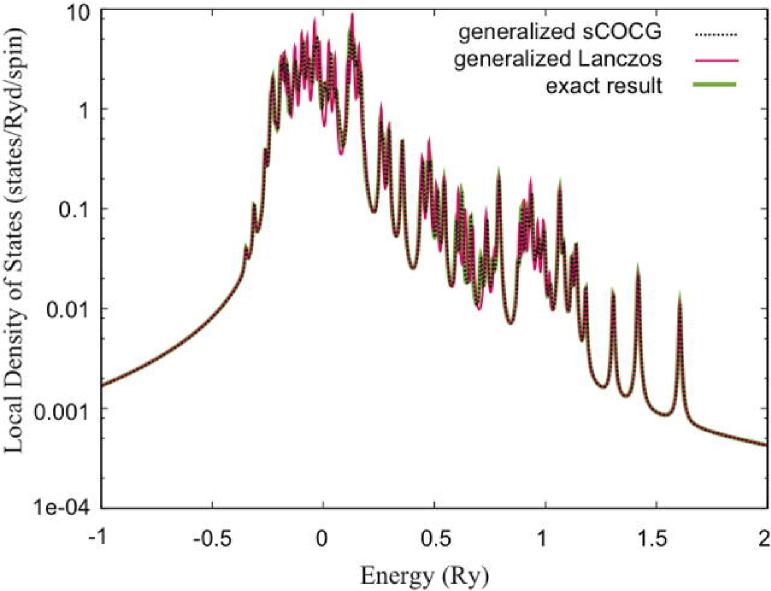
Figure 1: The local density of states of fcc gold of Au 256 atoms by the tb-LDA with non-orthogonal basis set. There are three lines in the figure and they are almost overlapped. The chemical potential locates at $+0.2947$ Ry.

3.4 Example

We have explained the generalized Lanczos method and the generalized shifted COCG method. Now we present the calculated results of the local density of states (LDOS) by using the tight-binding Hamiltonian with non-orthogonalized basis set given by the NRL Hamiltonian. [5] The system is of gold 256 atoms in a supercell of an fcc structure with s-, p-, and d-orbitals under a periodic boundary condition. Figure 1 shows the LDOS of d-orbitals, where the vertical axis is in logarithmic scale to see the behavior of tails. The three calculated results, the generalized Lanczos method, the generalized shifted COCG method and the exact calculation, are almost identical with each other.

The cpu times by a standard work-station of a single processor are 3.92 s, 21.20 s and 57.6 s for the generalized Lanczos method, the generalized shifted COCG and the exact calculation, respectively. The algorithm of the present developed algebraic methods is suitable for parallel computation. on the other hands, the cpu time grows as a cubic power of the matrix size in the exact calculation. Therefore, the present methods are promising in large scale electronic structure calculations.

4 Application to nano-scale systems

4.1 Scale-size dependence of recently developed linear algebraic methods

Much attention has been paid to nano-scale systems and the first principles molecular dynamics simulation has become more important in material sciences and engineering. We have developed a set of computational methods of electronic structure calculations, i.e. the generalized Wannier state methods, [20, 21, 22, 23] the Krylov subspace method, [24] and the shifted COCG method for nano-scale systems. [15] In the preceding sections, we have explained recent development on the ASED and generalized shifted COCG method. The tight-binding MD simulation method with being-developed linear algebraic algorithm is useful to achieve calculations in extra-large systems whose computational cost increases linearly proportional to the system size as shown in Fig.2, where tested examples are metallic, insulating and semiconducting dense materials.

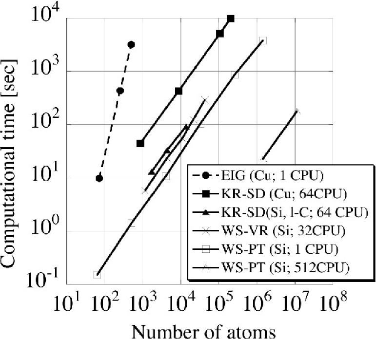
Figure 2: The computational time as a function of the number of atoms ($N$). [21, 22, 23] The time was measured in a older standard workstation for metallic (fcc Cu and liquid C) and insulating (bulk Si) systems with up to 11,315,021 atoms, by the conventional eigenstate calculation (EIG) and by our methods for large systems; KR-SD (Krylov subspace-diagonalization), WS-VR (Wannier-state variational) and WS-PT (Wannier-state perturbation) methods. The CPU time increases linearly with increasing the number of atoms. See the original papers [21, 22, 23] for the details of parallel computation.

4.2 Fracture propagation and surface reconstruction in silicon crystal

Here, we will show a calculation results of fracture propagation in a bulk Si single crystal with the semi-empirical tight-binding Hamiltonian by Kwon et al [1], based on the orthogonal basis set. The cleavage propagation speed is estimated, in the present model, as $v_{\rm prop}\simeq 2~{}{\rm nm/ps}=2~{}{\rm km/s}$, which is comparable to the velocity of the Rayleigh wave $v_{\rm R}=4.5~{}{\rm km/s}\simeq 4.5~{}{\rm nm/ps}$. [21, 22]

The easy-propagating plane of fracture in Si is known widely to be that of (110) or (111) and we studied the phenomena of fracture propagation in 14 nm scale Si crystals. [22] In case of fracture on the (111) plane, the the Pandy structure [25] of (111)-$(2\times 1)$ surface reconstruction appears with several steps. The direction or the structure of fracture propagation planes is not explained by the stabilization energy of the final stable surfaces structure because a transient surface structure is first formed immediately after the bond-breaking and, after appearance of the ideal surface, the surface reconstruction happens to form the final reconstructed surface. In the process of fracture propagation and surface reconstruction, the two different kinds of energy loss and gain compete with each other, e.g. the energy competition between an electronic energy gain of breaking bonds and an elastic energy loss of distorting the lattice. This kind competition may be possible only in nano-scale systems and, in a MD simulation, we should prepare larger systems, e.g. a few tens nm length. Then, even a fracture propagation starts on a (001) plane, the plane of the fracture propagation changes to (111) and (110) planes. Figure 3 shows examples of the surface reconstruction after formation of surfaces.

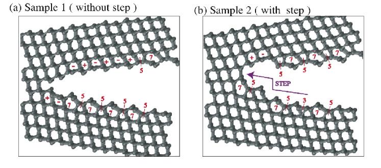
Figure 3: Fracture propagation on a (111) plane of a Si single crystal. (a) Appearance of Pandy structure without steps. (b) Pandy structure with a step. The numbers show the number of atoms in a ring. The symbols ($+$) or ($-$) refer to the electron charge, excess or deficiency.

4.3 Proton transfer in water

The correlation energy of water dimer, [26] hydrogen-bonded network [27] and protonated water [28] are all long-investigated problems of quantum chemistry. We have been applying the ASED method to water and proton transfer in water to investigate the applicability of the method.

The bond angle H-O-H (an experimental value 104.5^∘) is determined sensitively by the energy levels (binding energy and bond angle dependence) 1B₂ and 3A₁ of H₂O, which could be done by adjusting the ionic energy levels $\epsilon_{\rm 2s}$ and $\epsilon_{\rm 2p}$ of oxygen 2s and 2p orbitals and their STO parameters. After that, we could obtain the correct order of molecular energy levels of (2A₁), (1B₂), (3A₁), (1B₁), (4A₁), (2B₂) and an approximate cohesive energy of a molecule (10.97 eV, Cf. the experimental value of 10.08 eV). The bond length can be adjusted by slight rescaling the two-body repulsive term and the resultant bond length is 3.168Åand the CSC scheme works efficiently (Cf. 2.797Åwithout CSC scheme and 2.967Åby Gaussian B3LYP/6-31G(d,p)). Once we include H 2p state in the calculation, the molecular dimer configuration $\alpha=7^{\circ}$, $\beta=57^{\circ}$ can be obtained, which is in good agreement with the results of Gaussian calculation ($\alpha=6^{\circ}$ and $\beta=57^{\circ}$. See the inset in Fig. 4).

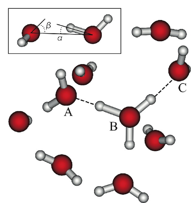
Figure 4: Snap shot of the proton transfer process. A proton transfers from a H₂O molecule A to that of B and another proton will transfer from the oxonium ion H₃O⁺ to that of C. The inset shows the definition of angles $\alpha$ and $\beta$ for a stable configuration of a water dimer.

Then we simulate the proton transfer in a water system 100H₂O + H₃O⁺ and observe the proton transfer process to happen in a recombination of H₃O⁺ + H₂O $\Rightarrow$ H₂O + H₃O⁺ (hopping of a proton) but not the transfer of an oxonium ion H₃O⁺ itself and the jumping time is of the order of 1 ps. Furthermore, we observe the following elementary process within an order of 0.1 ps;
(1) A H₃O⁺ ion tries to find a proper one in near-neighboring H₂O molecules,
(2) a H₃O⁺ ion forms a weak bond with one of H₂O (forming H₃O⁺+H₂O), and
(3) a proton transfers to that H₂O, forming H₂O+H₃O⁺.
(4) If this H₂O is proper one, the new H₂O molecule (the former H₃O⁺ ion) rotates (to form a stable water dimer 2H₂O) and change to a stable configuration and, at the same time,
(5) a new H₃O⁺ ejects a proton H⁺ to a next H₂O.

From these observation, we may conclude that the ASED framework can work properly in a wide variety of materials. The present system size of water is still too small to use the generalized Lanczos method and the generalized shifted COCG method. Even so, we have already assured these methods for working in the MD simulation in the present system.

5 Conclusions

We have reviewed our recently developed methods of ASED based on the generalized Hückel approximation and the novel linear algebraic algorithm for large-scale quantum molecular dynamics simulation. The crucial point is that the novel linear algebraic algorithm is applicable to systems of several thousand atoms or more with the same accuracy of the exact calculation. Then we presented examples of the applications to the fracture propagation and surface reconstruction in Si and the proton transfer in water. The water is very sensitive and difficult systems to simulate and the successful results suggest that our proposed simulation method is promising in a wide variety of systems, dense or dilute, solids, liquids or soft materials, and metals or insulators. The present MD simulation method was applied also to the problems of the formation of helical multishell Au nanowire [29] and the diamond-graphite transformation under applied stress [30].

References

References

- [1] I. Kwon, R. Biswas, C. Z. Wang, K. M. Ho, and C. M. Soukoulis, Phys. Rev. B 49, 7242 (1994).
- [2] P. Vogl, H. P. Hjalmarson, and J. D. Dow, J. Phys. Chem. Solids 44, 365 (1983).
- [3] O. K. Andersen and O. Jepsen, Phys. Rev. Lett. 53, 2571 (1984).
- [4] For example, D. Porezag, Th. Frauenheim, Th. Köhler, G. Seifert, and R. Kaschner, Phys. Rev. B 51, 12947 (1995).
- [5] M. J. Mehl and D. A. Papaconstantopoulos, Phys. Rev. B 54, 4519 (1996); F. Kirchhoff, M. J. Mehl, N. I. Papanicolaou, D. A. Papaconstantopoulos, and F. S. Khan, Phys. Rev. B 63, 195101 (2001).
- [6] K. Nath and A. B. Anderson, Phys. Rev. B 41, 5652 (1990).
- [7] M. Wolfsberg and L. J. Helmholz, J. Chem. Phys. 20, 837 (1952); R. Hoffmann, J. Chem. Phys. 39, 1397, (1963).
- [8] G. Calzaferri and R. Rytz, J. Phys. Chem. 100, 11122 (1996).
- [9] D. Porezag, Th. Frauenheim, Th. Köhler, G. Seifert, and R. Kaschner, Phys. Rev. B 51, 12947 (1995).
- [10] M. Elstner, D. Porezag, G. Jungnickel, J. Elsner, M. Haugk, Th. Frauenheim, S.Suhai and G. Seifert, Phys. Rev. B 58, 7260 (1998).
- [11] T. Fujiwara, T. Hoshi, and S. Yamamoto, J. Phys.: Condens. Matter 20, 294202 (2008); T. Fujiwara, T. Hoshi, S. Yamamoto, T. Sogabe, and S.-L. Zhang, J. Phys.: Condens. Matter 22, 074206 (2010).
- [12] H. Teng, T. Fujiwara, T. Hoshi, T Sogabe, S.-L. Zhang, and S. Yamamoto, in preparation.
- [13] H. A. van der Vorst and J. B. M. Melissen, IEEE Trans. Magn. 26, 706 (1990).
- [14] A. Frommer, Computing 70, 87 (2003).
- [15] R. Takayama, T. Hoshi, T. Sogabe, S-L. Zhang and T. Fujiwara, Phys. Rev. B 73, 165108 (2006).
- [16] T. Sogabe and S.-L. Zhang, talk in the International Conference Numerical Analysis and Scientific Computing with Applications, Agadir, Morocco, May 18-22, 2009.
- [17] T. Sogabe, T. Hoshi, S.-L. Zhang, and T. Fujiwara, Frontiers of Computational Science, pp. 189-195, Ed. Y. Kaneda, H. Kawamura and M. Sasai, (Springer Verlag, Berlin Heidelberg, 2007).
- [18] S. Yamamoto, T. Sogabe, T. Hoshi, S.-L. Zhang, and T. Fujiwara, J. Phys. Soc. Jpn 77, 114713 (2008).
- [19] T. Sogabe, T. Hoshi, S.-L. Zhang, and T. Fujiwara, Electronic Transactions on Numerical Analysis (ETNA), 31, 126 (2008).
- [20] T. Hoshi and T. Fujiwara, J. Phys. Soc. Jpn. 69, 3773 (2000).
- [21] T. Hoshi and T. Fujiwara, J. Phys. Soc. Jpn. 72, 2429 (2003).
- [22] T. Hoshi, Y. Iguchi and T. Fujiwara, Phys. Rev. B 72, 075323 (2005).
- [23] T. Hoshi, and T. Fujiwara, J. Phys: Condens. Matter. 18, 10787 (2006).
- [24] R. Takayama, T. Hoshi and T. Fujiwara, J. Phys. Soc. Jpn. 73, 1519 (2004).
- [25] K. C. Pandey, Phys. Rev. Lett. 47, 1913 (1981).
- [26] O. Matsuoka, E. Clementi, and M. Yoshimine, J. Chem. Phys. 64,1351 (1976).
- [27] S. Scheiner, Annu. Rev. Phys. Chern. 45, 23 (1994).
- [28] T. Wróblewskia, L. Ziemczoneka, E. Gazdaa, and G.P. Karwasza, Rad. Phys. Chem. 68, 313 (2003).
- [29] Y. Iguchi, T. Hoshi and T. Fujiwara, Phys. Rev. Lett. 99, 125507 (2007); T. Hoshi and T. Fujiwara, J. Phys. Condens. Matte 21, 272201 (2009);
- [30] T. Hoshi, T. Iitaka, and M. Fyta, J. Phys. Conf. Ser. 215, 012118 (2010)