Heat conduction: a telegraph-type model with
self-similar behavior of solutions

Abstract

For heat flux $q$ and temperature $T$ we introduce a modified Fourier–Cattaneo law $q_{t}+l\frac{q}{t}=-kT_{x}.$ The consequence of it is a non-autonomous telegraph-type equation. This model already has a typical self-similar solution which may be written as product of two travelling waves modulo a time-dependent factor and might play a role of intermediate asymptotics.

It is well known, that the heat equation propagates perturbations with infinite velocity. For this contradiction a possible answer is the telegraph equation which is ”obviously hyperbolic”. In general, one usually forgets about the other fundamental properties of parabolic heat equations: the existence of self-similar solutions (e.g., the Gaussian kernel or fundamental solution) and the attracting nature of these special solutions (intermediate asymptotics).

Is is easy to show, that the telegraph equation –see (5)–has no self-similar solutions e.g., solutions of the form $t^{-{\alpha}}f(x/t^{\beta})$ and that even asymptotic self-similarity property is lacking: no solutions of form $g(t)\cdot f(x/w(t))$ with $g\sim t^{-\alpha}$ and $h\sim t^{\beta}$ for $t>>1$.

Since the telegraph equation (possibly with reaction terms) supposed to be relevant not only in heat conduction but also in various diffusion processes, the lack in self-similarity might be a bad sign for the adequacy of the model. In addition, in diffusion and heat theory various physical quantities, like the fluxes, have to be continuous; therefore the solutions of this equation cannot be ”too bad”.

According to Gurtin and Pipkin gurt ; jos1 ; jos2 , the most general form of the flux in linear heat conduction and diffusion related to the flux $q$ expressed in one space dimension via an integral over the history of the temperature gradient

$$q=-\int_{-\infty}^{t}Q(t-t^{\prime})\frac{\partial T(x,t^{\prime})}{\partial x}dt^{\prime}$$ (1)

where $Q(t-t^{\prime})$ is a positive, decreasing relaxation function that tends to zero as $t-t^{\prime}\rightarrow\infty$ and $T(x,t)$ is the temperature distribution.

There are two notable relaxation kernel functions: if $Q(s)=k\delta(s)$ where $\delta(s)$ is a Dirac delta ”function”, then

$$q=-k\frac{\partial T(x,t)}{\partial x}$$ (2)

is the Fourier law.

If we define the kernel as $Q(s)=\frac{k}{\tau}e^{-s/\tau}$ where $s=t-t^{\prime}$ and $k$ is the constants of the effective thermal conductivity we get back to the well-known Cattaneo cat heat conduction law which reads:

$$\tau\frac{\partial{q}}{\partial t}+q=-k\frac{\partial T(x,t)}{\partial x}.$$ (3)

There is a third kind of relaxation kernel, the ”Jeffrey-type”, which applies both $Q(s)=k_{1}\delta(s)+\frac{k_{2}}{\tau}e^{-s/\tau}.$

The energy conservation law

$$\frac{\partial q}{\partial x}=-\gamma\frac{\partial T(x,t)}{\partial t},$$ (4)

where $\gamma$ is the heat capacity, gives the heat equation with (1) and the telegraph equation with (2):

$$\frac{\partial^{2}T(x,t)}{\partial t^{2}}+\frac{1}{\tau}\frac{\partial T(x,t)}{\partial t}=c^{2}\frac{\partial^{2}T(x,t)}{\partial x^{2}},$$ (5)

where $c=\sqrt{k/\tau\gamma}$ is the propagation velocity of the transmitted heat wave. The flux $q$ satisfies the same equation.

The thermal diffusivity $\kappa=k/\gamma$ can be defined as the ratio of the effective thermal conductivity $k$ and the heat capacity $\gamma$. This equation describes a physical process with a well defined relaxation time $\tau$.

The telegraph equation (5) can be derived in various transport systems. First it was derived by Kirchhoff to describe the voltage on a realistic electrical transmission line with distance and time, this derivation can be found in any textbook on electrodynamics. Later Goldstein gold derived the telegraph equation from a generalized random walk for diffusion. Okubo okubo summarized the knowledge of the telegraph equation till 1971 and presented a new ad-hoc derivation for turbulent mixing his starting point being the Navier-Stokes system. In all these derivations the $\tau$ relaxation time had a well-established physical meaning presenting the time-scale of the physical process. Joseph and Preziosi collected basically all the relevant works done on heat waves connected with the telegraph equation till 1990 jos1 ; jos2 . On the other side the telegraph equation was intensively investigated from the mathematical point of view as well othm . Different kind of properties of these models can be analyzed as in kers .
In the present communication we introduce a new kernel which somehow interpolates the Dirac delta and the exponential kernel having the main properties of both. The $Q(s)=1/s^{l}$ is such a function: it is singular at the origin and has a short range of decay for $l>1$. Let’s consider the following relaxation kernel

$$Q(t-t^{\prime})=\frac{k\tau^{l}}{(t-t^{\prime}+\omega)^{l}}$$ (6)

where $k$ is the effective thermal conductivity, $\tau$ is a relaxation time and $l>1$ is a parameter, $-t^{\prime}+\omega$ is just a time shift which is needed to regularize the expression.

Using the general form of heat flux (1) we get

$$q=-\int_{-\infty}^{t}\frac{k\tau^{l}}{(t-t^{\prime}+\omega)^{l}}\frac{\partial T(x,t)}{\partial x}dt^{\prime}.$$ (7)

One has

$$\frac{\partial q}{\partial t}=-k\left(\frac{\tau}{\omega}\right)^{l}\frac{\partial T(x,t)}{\partial x}+$$

$$l\int_{-\infty}^{t}\frac{1}{t-t^{\prime}+\omega}\frac{k\tau^{l}}{(t-t^{\prime}+\omega)^{l}}\frac{\partial T(x,t^{\prime})}{\partial x}dt^{\prime}.$$ (8)

A formal application of integral mean theorem to the second term on the right hand side and the definition of $q$ leads to a new phenomenological law

$$\frac{\partial q}{\partial t}=-k\left(\frac{\tau}{\omega}\right)^{l}\frac{\partial T(x,t)}{\partial x}-\frac{l}{t-t^{\prime\prime}+\omega}q.$$ (9)

The additional energy conservation law is still (4) and from this and the last equation we obtain

$$\frac{\gamma}{k}\left(\frac{\omega}{\tau}\right)^{l}\frac{\partial^{2}T(x,t)}{\partial t^{2}}+$$

$$\frac{\gamma}{k}\left(\frac{\omega}{\tau}\right)^{l}\frac{l}{t-t^{\prime\prime}+\omega}\frac{\partial T(x,t)}{\partial t}=\frac{\partial^{2}T(x,t)}{\partial x^{2}}.$$ (10)

For a better transparency let’s call $\epsilon=\frac{\gamma}{k}\left(\frac{\omega}{\tau}\right)^{l}$ and $a=\frac{\gamma}{k}\left(\frac{\omega}{\tau}\right)^{l}\cdot l$ The physical meaning of $\epsilon$ is still the thermal diffusivity multiplied by a scaling constant which is the renormalized relaxation time (the ratio of an ordinary time shift $\omega$ and a well defined relaxation time $\tau$). The exponential $l$ is a real number which describes the non-locality in time which we may call memory effects of the heat conduction phenomena. Larger $l$ means shorter memory. The physical meaning of $a$ is approximately the thermal diffusivity multiplied by another time-scaling factor. In the following we will see that the role of $a,\epsilon$ or $l$ will be crucial in the structure of the solutions. At last we introduce a new time variable $t=t-t^{\prime\prime}+\omega.$ Now our telegraph-type equation reads

$$\epsilon\frac{\partial^{2}T(x,t)}{\partial t^{2}}+\frac{a}{t}\frac{\partial T(x,t)}{\partial t}=\frac{\partial^{2}T(x,t)}{\partial x^{2}}.$$ (11)

Note, that the $a/t$ factor appearing in front of the first time derivate makes the equation time-reversible, which cannot be true for diffusion or heat propagation processes, at the same time the $a/t$ factor makes the equation irregular at the origin. To avoid these problems, we may shift the pole to a negative time value - in practical calculations using the $a/(t+\tau)$ where $\tau$ still can be any kind of relaxation time with well-founded physical interpretation. Physically it is clear, if a process has a well-defined time-scale than the reverse process cannot run back in time more than the physically relevant time. Now, in this sense, for positive time $(t>0)$ we may use the equation to describe diffusion-like processes. Our deeper investigation clearly shows, that no other exponent of $t$ as one can have self-similar solution.

If we consider (11) as a non-linear wave equation we may investigate wave properties like dispersion phenomena. Inserting the standard plain wave approximation $T(x,t)=e^{i(\tilde{k}x+\tilde{\omega}t)}$ into (11) the dispersion relation and the attenuation distance can be obtained. These are the followings:

$$v_{p}=\frac{\tilde{\omega}}{Re(\tilde{k})}=\sqrt{\frac{2}{\epsilon}}{\tilde{\omega}}\left(1+\sqrt{1+\left(\frac{l}{t}\right)^{2}}\right)^{-1/2}\hskip 8.5359pt\tilde{\alpha}=\frac{1}{Im(\tilde{k})}=\frac{2t}{\epsilon l}\frac{1}{v_{p}}.$$ (12)

Our telegraph-type equation is time dependent, hence both the dispersion relation and the attenuation distance have time dependence. Note, that $v_{p}$ has a very weak time-dependence, basically only till $t\leq l$. As an other interesting point is that the phase velocity does not depend on the angular velocity which is the same as for the ideal wave equation, so our equation has no dispersion. So in this sense our equation is very similar to the wave-equation, which is hyperbolic. The properties of the attenuation distance is even more interesting, it is divergent in time and has a $1/\tilde{\omega}$ angular frequency. However if we let the angular frequency and the time to go infinite with the same speed than the attenuation distance has a strong decay. Which is like the skin-effect when high frequency electrons can only propagate on the surface of a metal.

We are looking for solution of (11) of the form

$$T(x,t)=t^{-\alpha}f\left(\frac{x}{t^{\beta}}\right):=t^{-\alpha}f(\eta).$$ (13)

The similarity exponents $\alpha$ and $\beta$ are of primary physical importance since $\alpha$ represents the rate of decay of the magnitude $T(x,t)$, while $\beta$ is the rate of spread (or contraction if $\beta<0$ ) of the space distribution as time goes on. Substituting this into (11) we have

$$f^{\prime\prime}(\eta)t^{-\alpha-2}[\epsilon\beta^{2}\eta^{2}]+$$

$$f^{\prime}(\eta)\eta t^{-\alpha-2}[\epsilon\alpha\beta-\epsilon\beta(-\alpha-\beta-1)-\beta a]+$$

$$f(\eta)t^{-\alpha-2}[-\epsilon\alpha(-\alpha-1)-a\alpha]=f^{\prime\prime}(\eta)t^{-\alpha-2\beta},$$ (14)

where prime denotes differentiation with respect to $\eta.$

One can see that this is an ordinary differential equation(ODE) if and only if $\alpha+2=\alpha+2\beta$ (the universality relation). So it has to be

$$\beta=1$$ (15)

while $\alpha$ can be any number. The corresponding ODE we shall deal with is

$$f^{\prime\prime}(\eta)[\epsilon\eta^{2}-1]+f^{\prime}(\eta)\eta(2\epsilon\alpha+2\epsilon-a)+f(\eta)\alpha(\epsilon\alpha+\epsilon-a)=0.$$ (16)

In pure heat conduction-diffusion processes–no sources or sinks–the heat mass is conserved: the integral of $T(x,t)$ with respect to $x$ does not depend on time $t$. For $T(x,t)$ this means

$$\int T(x,t)dx=t^{-\alpha}\int f(\frac{x}{t})dx=t^{-\alpha+1}\int f(\eta)d\eta=const$$ (17)

if and only if $\alpha=1.$ We are going to investigate this case only. Plainly (19) can be written as

$$(\varepsilon f\eta^{2}-f)^{\prime\prime}=a(\eta f)^{\prime}$$ (18)

which after integration and supposing $f(\eta_{0})=0$ for some $\eta_{0}$ gives

$$\frac{df}{f}=\frac{a\eta d\eta}{\varepsilon\eta^{2}-1}.$$ (19)

From this equation we can obtain two qualitatively different solutions. The one which is globally bounded and positive in the domain $\{(x,t):1-\varepsilon\eta^{2}>0\}$ and has the form

$$f=(1-\varepsilon\eta^{2})^{\frac{a}{2\varepsilon}-1}_{+}$$ (20)

where $(f)_{+}=\max(f,0).$ See Fig. (1).

The corresponding self-similar solution is

$$T(x,t)=\frac{1}{t}\left(1-\varepsilon\frac{x^{2}}{t^{2}}\right)^{\frac{a}{2\varepsilon}-1}_{+}$$ (21)

This solution is positive in the cone $t^{2}>\varepsilon x^{2}$ and is zero outside of it, see Fig. (2). Note, that only the $x>0$ and $t>0$ quarter of the plane is presented, because of it has physical relevance.

*

Figure 1: Eq. (21) thick solid line is for $l=6.2$ and the thin dashed line is for $l=4.1$.

On the $(x,t)$ plane there are two fronts $x(t)=\pm\frac{t}{\sqrt{\varepsilon}}$ separating these domains. Because the function $T(x,t)$ not always has continuous derivatives entering to (11) we have to make clear what we mean under ”solution”. Having in mind the physical background, we ask the continuity of $T_{t},T_{x},q_{t}$ and $q_{x}$ so that in (2) and (3) all functions were continuous.

*

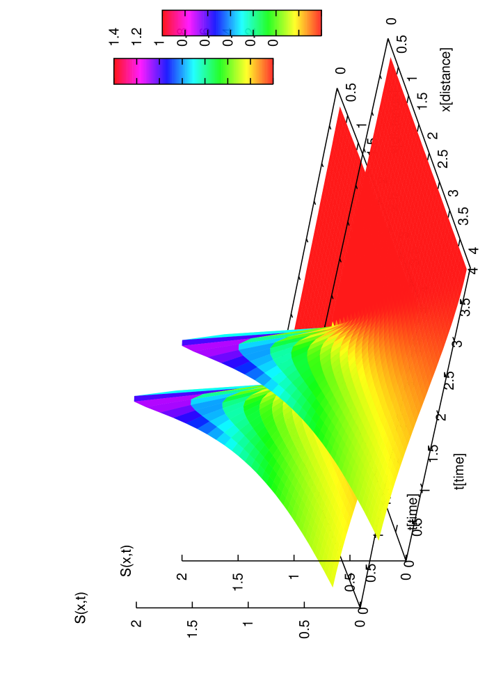
Figure 2: The solution (21) for the parameter $l=6.2$.

In our case this means that

$$\frac{a}{2\varepsilon}-1=\frac{l-2}{2}$$ (22)

has to be greater than $1$, i.e. $a/\varepsilon=l>4,$ which we shall suppose further on. If the second derivatives are not continuous ($4<l\leq 6$) we understand the solution in the sense of distributions. If $l>6$ the solution is classical. On Fig. 1. we compare the solutions with $l=4.1$ and $l=6.2$. the thick solid line represents the solution for $l=6.2$ and the thin dashed line however shows the solution for $l=4.1$.

Remark 1. The solution (21) is of source-type i.e. $\lim_{t\rightarrow 0}T(x,t)=K\delta(x),$ where $\delta$ is the Dirac measure, $K>0$. One can calculate the second initial condition $\lim_{t\rightarrow 0}T_{t}(x,t)$ too.

Remark 2. One can write (21) in the form of product of two traveling waves propagating in opposite direction (divided by a time-factor):

$$T(x,t)=\frac{1}{t^{l-1}}(t-\sqrt{\varepsilon}x)_{+}^{\frac{l}{2}-1}(t+\sqrt{\varepsilon}x)_{+}^{\frac{l}{2}-1}$$ (23)

which is a new-type of purely hyperbolic wave; the typical solution of the wave equation is the sum of two such waves: $g(x-ct)+g(x+ct)$.

It is known that an another possible answer to contradiction connected with the infinite speed of propagation is the nonlinear Fourier law ($\tau=0,k=k_{0}T^{m-1}$ in (2)) which leads to a nonlinear heat equation

$$T_{t}=(T^{m})_{xx},\quad m>1.$$ (24)

In zk Zeldovich and Kompaneets have found the fundamental solution $T_{1}$ of this equation which we write in the following form:

$$T_{1}^{m-1}=t^{-\alpha(m-1)}\left(A^{2}-B^{2}x^{2}t^{-2\beta}\right)_{+}=$$

$$\frac{1}{t}(At^{\beta}-Bx)_{+}(At^{\beta}+Bx)_{+},$$ (25)

where $A$ is constant and

$$\alpha=\beta=\frac{1}{m+1},\quad B^{2}=\frac{m-1}{2m(m+1)}.$$ (26)

One can see that this solution has bounded support in $x$ for any $t>0$ which is a hyperbolic property. Using comparison principle for such equations one can show this finite speed property for any initial condition having compact support. However, the fronts are not straight lines: $x(t)=\pm\frac{A}{B}t^{\beta}$, $\beta<1$ so the speed of propagation $\dot{x}(t)$ goes to zero if $t$ goes to infinity. One can also see that $T_{1}$ is of source-type: $T_{1}(x,0)=K_{1}\delta(x).$

The most intrinsic property of $T_{1}$ is that it plays the role of intermediate asymptotic: any solution of (24) corresponding to the initial datum $t(x,0)$ with $\int t(x,0)dx=K_{1}$ converges to $T_{1}$ as $t\rightarrow\infty.$ This was conjectured earlier but was shown only in 1973 by Sh. Kamin, see ka .

It would be important and interesting to understand whether or not our special solution $T(x,t)$ had this attractor property. If ”yes”, in what sense: we recall that there is a second initial condition too.

In summary. - We introduced a new phenomenological law for heat flux which in some sense ”interpolates” between Fourier and Cattaneo laws. The consequence of it is a non-autonomous model, a telegraph-type partial differential equation. It already has, unlike the classical telegraph equation, self-similar solutions, the presence of which is desirable in the theory of heat propagation free from sources and absorbers.

One of us (R.K.) would like to thank Prof. P. Rosenau for his stimulating discussion.

References

- (1) M.E. Gurtin and A.C. Pipkin, Arch. Ration. Mech. Anal. 31, 113 (1968).
- (2) D.D. Joseph and L. Preziosi, Rev. Mod. Phys. 61, 41 (1989).
- (3) D.D. Joseph and L. Preziosi, Rev. Mod. Phys. 62, 375 (1990).
- (4) C. Cattaneo, Sulla conduzione del calore Atti. sem Mat. Fis. Univ. Modena 3, 83 (1948).
- (5) S. Goldstein, Quart. J. Mech. and Appl. Math. 4, 129 (1951).
-
(6)
A. Okubo, Application of the Telegraph Equation to Oceanic
Diffusion: Another Mathematical Model Chesapeake Bay
Institute, The John Hopkins University, Technial
Report 69, N00014-67-A-0163-0006 NR 083-016
http://dspace.udel.edu:8080/dspace/handle/19716/1439. - (7) H.G. Othmer, S.R. Dunbar and W. Alt, J. Math. Biol. 26, 263 (1988).
- (8) B.H. Gilding and R. Kersner, Travelling Waves in Nonlinear Diffusion-Convection Reactions, Progress in Nonlinear Differential Equations and Their Applications, Birkhäuser Verlag, Basel-Boston-Berlin, 2004, ISBN 3-7643-7071-8.
- (9) Sh. Kamin, Israeli Journal of Maths, 14, 76 (1973).
- (10) Y.B. Zeldovich and A.S. Kompaneets, Collection Dedicated to the 70th Birthday of A.F. Joffe, Izdat. Akad. Nauk SSSR 1950, p.61.