Metallicity as a source of dispersion in the SNIa bolometric light curve luminosity-width relationship

Abstract

The recognition that the metallicity of Type Ia supernova (SNIa) progenitors might bias their use for cosmological applications has led to an increasing interest in its role on the shaping of SNIa light curves. We explore the sensitivity of the synthesized mass of ⁵⁶Ni, $M(^{56}\mathrm{Ni})$, to the progenitor metallicity starting from Pre-Main Sequence models with masses $M_{0}=2-7$ M_⊙ and metallicities $Z=10^{-5}-0.10$. The interplay between convective mixing and carbon burning during the simmering phase eventually rises the neutron excess, $\eta$, and leads to a smaller ⁵⁶Ni yield, but does not change substantially the dependence of $M(^{56}\mathrm{Ni})$ on $Z$. Uncertain attributes of the WD, like the central density, have a minor effect on $M(^{56}\mathrm{Ni})$. Our main results are: 1) a sizeable amount of ⁵⁶Ni is synthesized during incomplete Si-burning, which leads to a stronger dependence of $M(^{56}\mathrm{Ni})$ on $Z$ than obtained by assuming that ⁵⁶Ni is produced in material that burns fully to nuclear statistical equilibrium (NSE); 2) in one-dimensional delayed detonation simulations a composition dependence of the deflagration-to-detonation transition (DDT) density gives a non-linear relationship between $M(^{56}\mathrm{Ni})$ and $Z$, and predicts a luminosity larger than previously thought at low metallicities (however, the progenitor metallicity alone cannot explain the whole observational scatter of SNIa luminosities), and 3) an accurate measurement of the slope of the Hubble residuals vs metallicity for a large enough data set of SNIa might give clues to the physics of deflagration-to-detonation transition in thermonuclear explosions.

1 Introduction

In addition to the mass, metallicity is one of the few progenitor attributes that can leave an imprint on the observational properties of SNIa by affecting the synthesized mass of ⁵⁶Ni, with important consequences for their use as cosmological standard candles. Up to now, attempts to measure $Z$ directly from supernova observations have been scarce and their results uncertain (Lentz et al., 2000; Taubenberger et al., 2008). Measuring $Z$ from the X-ray emission of supernova remnants is a promising alternative but as yet has been only applied to a single supernova (Badenes et al., 2008). An alternative venue is to estimate the supernova metallicity as the mean $Z$ of its environment (Badenes et al., 2009). Hamuy et al. (2000) looked for galactic age or metal content correlations with SNIa luminosity, but their results were ambiguous. Ellis et al. (2008) looked for systematic trends of SNIa UV spectra with metallicity of the host galaxy, and found that the spectral variations were much larger than predicted by theoretical models. Cooper et al. (2009), using data from the Sloan Digital Sky Survey and Supernova Survey concluded that prompt SNIa are more luminous in metal-poor systems. Recently, Gallagher et al. (2008, hereafter G08) and Howell et al. (2009, hereafter H09), using different methodologies to estimate the metallicity of SNIa hosts, arrived to opposite conclusions with respect to the dependence of supernova luminosity on $Z$.

There is a long history of numerical simulations of SNIa aimed at predicting the impact of metallicity and explosive neutronization on their yields (e.g. Bravo et al., 1992; Brachwitz et al., 2000; Travaglio et al., 2005; Badenes et al., 2008). Domínguez et al. (2001, hereafter DHS01) found that the offset in the calibration of supernova magnitudes vs light curve (LC) widths is not monotonic in $Z$ and remains smaller than $0.07^{\mathrm{m}}$ for $Z\leq 0.02$. Kasen et al. (2009) concluded that the width-luminosity relationship depends weakly on the metallicity of the progenitor. From an analytical point of view, Timmes et al. (2003, hereafter TBT03) using arguments from basic nuclear physics predicted a linear relationship between $M(^{56}\mathrm{Ni})$ and $Z$. The conclusions of TBT03 relied on two main assumptions: first, that most of the ⁵⁶Ni is synthesized in material that burns fully to NSE and, second, that a fiducial SNIa produces a mass $M_{\mathrm{Fe}}^{\eta_{0}}\sim 0.6$ M_⊙ of Fe-group nuclei whose $\eta$ is not modified during the explosion. Piro & Bildsten (2008) and Chamulak et al. (2008), based on the same assumptions as TBT03, extended their analysis taking into account the neutronization produced during the simmering phase.

In this paper, we show that the first assumption of TBT03 does not hold for most SNIa. Indeed, for a SNIa that produces $M_{\mathrm{Fe}}^{\eta_{0}}\sim 0.6$ M_⊙ the fraction of ⁵⁶Ni synthesized out of NSE exceeds $\sim 30\%$. With respect to the second assumption, Mazzali et al. (2007, hereafter M07) showed, based on observational results, that the mass of Fe-group nuclei ejected by SNIa spans the range from 0.4 to 1.1 M_⊙. This range cannot be accounted for by metallicity variation within reasonable values. Accordingly, our working hypothesis is that the yield of ⁵⁶Ni in SNIa is governed by a primary parameter different from $Z$. In our one-dimensional models the primary parameter is the DDT density, $\rho_{\mathrm{DDT}}$, although in nature it may be something else such as the expansion rate during the deflagration phase. The initial metallicity is a secondary factor that can give rise to scatter in the value of $M(^{56}\mathrm{Ni})$ either directly (linear scenario), by affecting the chemical composition of the ejecta for a given value of the primary parameter, or indirectly (non-linear scenario), by modifying the primary parameter itself. The understanding of which one of these two characters is actually being played by $Z$ is of paramount importance.

2 The effect of metallicity on the yield of ⁵⁶Ni

We explore the sensitivity of $M(^{56}\mathrm{Ni})$ to the progenitor metallicity, starting from Pre-Main Sequence models of masses, $M_{0}$, in the range $2-7$ M_⊙ and metallicities, $Z$, from $10^{-5}$ to 0.10, as given in the first column of Table 1. The initial mass fractions of all the isotopes with $A\gtrsim 6$ have been fixed in solar proportion, according to Lodders (2003); consequently, we adopt for the solar metallicity the value $Z_{\odot}=0.014$. Each presupernova model has been evolved from the Pre-Main Sequence to the Thermal Pulse (TP) AGB phase, in order to determine the mass, $M_{\mathrm{core}}$, and chemical structure of the C-O core left behind. Afterwards, an envelope of the appropriate size to reach the Chandrasekhar mass, $M_{\mathrm{Ch}}$, has been added on top of the C-O cores, and these structures have been fed as initial models to a supernova hydrocode. Finally, the explosive nucleosynthesis has been obtained with a post-processing nucleosynthetic code.

The hydrostatic evolution has been computed by means of the FRANEC code (Chieffi et al., 1998). With respect to the calculations of DHS01, the code has been updated in the input physics. For the purposes of the present paper, the most important changes concern the ${}^{12}\mathrm{C}\left(\alpha,\gamma\right)^{16}\mathrm{O}$ reaction rate, which is calculated according to Kunz et al. (2002) instead of Caughlan et al. (1985), and the treatment of convective mixing during the late part of the core-He burning (Straniero et al., 2003).

The presupernova model is a Chandrasekhar mass WD built in hydrostatic equilibrium with a central density $\rho_{\mathrm{c}}=3\times 10^{9}$ g cm^-3. The composition of the envelope of mass $M_{\mathrm{Ch}}-M_{\mathrm{core}}$ is the same as that of the outermost shell of the C-O core. Thus, instead of assuming C/O=1, as in DHS01, we adopt the C/O ratio obtained as a result of He-shell burning during the AGB phase. The effect of changing $\rho_{\mathrm{c}}$ and the composition of the envelope has been tested in several models, as explained later. We leave aside other eventual complexities of pre-supernova physics like rotation (Piersanti et al., 2003; Yoon & Langer, 2004).

The internal composition of the WD is eventually modified during the simmering phase, due to the combined effects of convective mixing, carbon burning and electron captures. The first two phenomena affect the carbon abundance within the core, while the latter leads to an increase of $\eta$. The average (within the WD) carbon consumption and neutron excess increase during the simmering phase are $\Delta Y(^{12}\mathrm{C})\approx-1.66\times 10^{-3}$ mol g^-1 and $\Delta\eta=-\frac{2}{3}\Delta Y(^{12}\mathrm{C})$ (Chamulak et al., 2008). We assume that convective mixing is limited to the C-O core, which implies that the change in the neutron excess within the core is $\Delta\eta\approx 1.11\times 10^{-3}M_{\mathrm{Ch}}/M_{\mathrm{core}}$. We have also exploded several models disregarding the simmering phase, to which we will refer in the following as stratified models.

The supernova hydrodynamics code we have used is the same as in Badenes et al. (2003). As in DHS01, the present models are based on the delayed-detonation paradigm (Khokhlov, 1991). To address the linear scenario we take $\rho_{\mathrm{DDT}}$ independent of $Z$. In this case, $\rho_{\mathrm{DDT}}=3\times 10^{7}$ g cm^-3, although simulations with $\rho_{\mathrm{DDT}}$ in the range $1-3\times 10^{7}$ g cm^-3 are also reported.

For the non-linear scenario we have adopted the criterion that a DDT is induced when the laminar flame thickness, $\delta_{\mathrm{lam}}$, becomes of the order of the turbulent Gibson length $l_{\mathrm{G}}$ (Röpke & Niemeyer, 2007), with the flame properties (velocity and width) depending on the abundances of ¹²C (eq. 22 in Woosley, 2007) and ²²Ne (Chamulak et al., 2007), and hence on $Z$ and $\eta$. Townsley et al. (2009) concluded from 2D simulations of SNIa that the metallicity does not affect the dynamics of the explosion, and so the turbulence intensity is independent of $Z$. Thus, for a given turbulent intensity a change in $Z$ can be compensated by a change in $\rho_{\mathrm{DDT}}$ in order to recover the condition $\delta_{\mathrm{lam}}/l_{\mathrm{G}}\approx 1$ (see the discussion in Chamulak et al., 2007). In this scenario we have scaled the transition density as a function of the local chemical composition as follows:

$$\rho_{\mathrm{DDT}}\propto X(^{12}\mathrm{C})^{-1.3}\left(1+129\eta\right)^{-0.6}\,.$$ (1)

In order to introduce an $\eta$ dependence in the above expression we have assumed, for simplicity, that the bulk of neutronized isotopes synthesized during the simmering phase accelerates the carbon consumption rate the same way ²²Ne does.

2.1 Presupernova evolution

The results of the hydrostatic evolution of our presupernova models are shown in Table 1. For each $M_{0}$ and $Z$ we give: $M_{\mathrm{core}}$, the central abundance of ¹²C and $\eta$ in stratified models, $X_{\mathrm{c}}(^{12}\mathrm{C})$ and $\eta_{\mathrm{c}}$, and the same quantities in the models accounting for the simmering phase, $X_{\mathrm{sim}}(^{12}\mathrm{C})$ and $\eta_{\mathrm{sim}}$. In comparison with DHS01, the present models span a larger range of $Z$, as DHS01 computed models with $Z\lesssim Z_{\odot}$. In the common range of $Z$ and $M_{0}$ the results are comparable, although the adopted rate of the ${}^{12}\mathrm{C}\left(\alpha,\gamma\right)^{16}\mathrm{O}$ reaction leads to a slightly larger carbon abundance than in DHS01. The differences in $M_{\mathrm{core}}$ between our models and those of DHS01 are smaller than $0.06$ M_⊙. The central carbon to oxygen ratio and $M_{\mathrm{core}}$ we obtain, and their dependencies with $Z$ and $M_{0}$, agree as well with Umeda et al. (1999).

2.2 Mass of $M(^{56}\mathrm{Ni})$ ejected

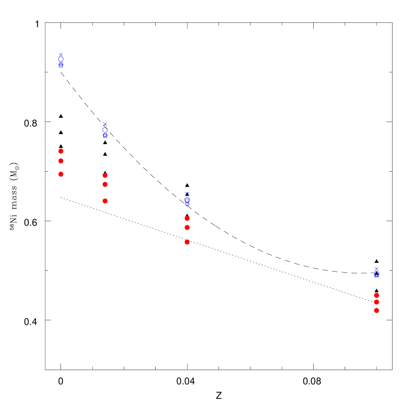
Figure 1: ⁵⁶Ni yield vs initial metallicity for different initial masses and explosion parameters. Black triangles: stratified models with $\rho_{\mathrm{c}}=3\times 10^{9}$ g cm^-3 and $\rho_{\mathrm{DDT}}=3\times 10^{7}$ g cm^-3. Red (filled) circles: models exploded with the same parameters but accounting for the simmering phase. Blue (empty) circles: the same as red circles except that $\rho_{\mathrm{DDT}}$ is a function of the local (at flame position) $Z$ through $X(^{12}\mathrm{C})$ and $\eta$ (Eq. 1) . Blue crosses and blue stars: the same as blue circles except that $\rho_{\mathrm{c}}=2\times 10^{9}$ g cm^-3 (crosses) or $\rho_{\mathrm{c}}=4\times 10^{9}$ g cm^-3 (stars). Blue squares: the same as blue circles except that the composition of the envelope is composed by equal amounts of carbon and oxygen, i.e. C/O = 1 as compared to values ranging from C/O = 1.5 to 2.3 as taken from the He-shell burning during the TP phase. The lines represent the linear relationship between $M(^{56}\mathrm{Ni})$ and $Z$ proposed in TBT03 (dotted line), and our Eq. 3 (dashed line).

The results of the explosion simulations are summarized in Figs. 1 and 2. Figure 1 shows the dependence of $M(^{56}\mathrm{Ni})$ on $Z$. For the stratified models, we obtain the same range of variation of $M(^{56}\mathrm{Ni})$ with respect to $M_{0}$ at given $Z$ as DHS01: 0.06 M_⊙, although the ${}^{56}\mathrm{Ni}$ yields do not match with DHS01 because they used different values of $\rho_{\mathrm{c}}=2\times 10^{9}$ g cm^-3 and $\rho_{\mathrm{DDT}}=2.3\times 10^{7}$ g cm^-3. The models accounting for the simmering phase behave like the stratified models with respect to variations in $M_{0}$ and $Z$, although with a smaller total $M(^{56}\mathrm{Ni})$ due to electron captures during the simmering phase. The dependence of $M(^{56}\mathrm{Ni})$ on $Z$ can be approximated by a linear function:

$$M(^{56}\mathrm{Ni})\propto f(Z)=1-0.075\frac{Z}{Z_{\odot}}\,,$$ (2)

while stratified models can be approximated by: $M(^{56}\mathrm{Ni})\propto 1-0.069Z/Z_{\odot}$, i.e. the slope of the linear function is quite insensitive to the carbon simmering phase.

To explore the non-linear scenario we have computed models accounting for the simmering phase with fixed $M_{0}=5$ M_⊙. Introducing a composition dependent $\rho_{\mathrm{DDT}}$ produces a qualitatively different result because the relationship between $M(^{56}\mathrm{Ni})$ and $Z$ is no longer linear, especially at low metallicites for which a larger $\rho_{\mathrm{DDT}}$ is obtained, implying a much larger $M(^{56}\mathrm{Ni})$. Our results can be fit by a polinomial law:

$$M(^{56}\mathrm{Ni})\propto f(Z)=1-0.18\frac{Z}{Z_{\odot}}\left(1-0.10\frac{Z}{Z_{\odot}}\right)\,.$$ (3)

Both the central density at the onset of thermal runaway and the final C/O ratio in the accreted layers have a minor effect on $M(^{56}\mathrm{Ni})$ within the explored range.

TBT03 proposed a linear relationship between $M(^{56}\mathrm{Ni})$ and $Z$: $M(^{56}\mathrm{Ni})\propto 1-0.057Z/Z_{\odot}$ (dotted line in Fig. 1). In all of our present models we find a steeper slope. The reason for this discrepancy lies in the assumption by TBT03 that most of the ⁵⁶Ni is synthesized in NSE. In our models a sizeable fraction of ⁵⁶Ni is always synthesized during incomplete Si-burning, whose final composition has a stronger dependence on $Z$ than NSE matter. As Hix & Thielemann (1996) showed, the mean neutronization of Fe-peak isotopes during incomplete Si-burning is much larger than the global neutronization of matter because neutron-rich isotopes within the Si-group are quickly photodissociated, providing free neutrons that are efficiently captured by nuclei in the Fe-peak group, favouring their neutron-rich isotopes. Figure 2 shows that up to $\sim 60\%$ of $M_{\mathrm{Fe}}^{\eta_{0}}$ can be made out of NSE, the actual fraction depending essentially on the total mass of Fe-group elements ejected. Thus, the less $M(^{56}\mathrm{Ni})$ is synthesized, the larger fraction of it is built during incomplete Si-burning and the stronger is its dependence on $Z$.

3 Discussion

The results presented in the previous section show that the metallicity is not the primary parameter that allows to reproduce the whole observational scatter of $M(^{56}\mathrm{Ni})$, for a reasonable range of $Z$. We have also shown that a possible dependence of the primary parameter on $Z$, would lead to a non-linear relationship between $M(^{56}\mathrm{Ni})$ and $Z$, as in Eq. 3. However, as we will show in the following, it would be possible to unravel the way $M(^{56}\mathrm{Ni})$ depends on $Z$ by means of future accurate measurements of SNIa properties.

We start analysing the amount of the scatter induced by the dependence of $M(^{56}\mathrm{Ni})$ on $Z$ given by Eq. 3. For simplicity we follow the procedure of M07 to estimate the supernova luminosity and LC width. The peak bolometric luminosity, $L$, is determined directly by the mass of ⁵⁶Ni synthesized (in the following, all masses are in $M_{\odot}$ and energies are in $10^{51}$ ergs):

$$L\left[M(^{56}\mathrm{Ni})\right]=2\times 10^{43}M(^{56}\mathrm{Ni})~{}\mathrm{erg}~{}\mathrm{s}^{-1}\,,$$ (4)

while the bolometric LC width, $\tau$, is determined by the kinetic energy, $E_{\mathrm{k}}$, and the opacity, $\kappa$: $\tau\propto\kappa^{1/2}E_{\mathrm{k}}^{-1/4}$. The kinetic energy is given by the difference of the WD initial binding energy, $\mathrm{|BE|}$, and the nuclear energy released, the latter being related to the final chemical composition of the ejecta: $E_{\mathrm{k}}\approx 1.56M(^{56}\mathrm{Ni})+1.74\left[M_{\mathrm{Fe}}-M(^{56}\mathrm{Ni})\right]+1.24M_{\mathrm{IME}}-\mathrm{|BE|}$ , where $M_{\mathrm{Fe}}$ is the total mass of Fe-group nuclei and $M_{\mathrm{IME}}$ is the mass of intermediate-mass elements (IME). The opacity is provided mainly by Fe-group nuclei and IMEs: $\kappa\propto M_{\mathrm{Fe}}+0.1M_{\mathrm{IME}}$. We have taken $\mathrm{|BE|}=0.46$, which is a good approximation given the small variation of binding energy with initial central density: $\mathrm{|BE|}$ is in the range $0.44-0.47$ for $\rho_{\mathrm{c}}=2-4\times 10^{9}$ g cm^-3. To reduce the number of free parameters we further link $M_{\mathrm{IME}}$ to $M_{\mathrm{Fe}}$ imposing that the ejected mass is the Chandrasekhar mass ($M_{\mathrm{Ch}}\approx 1.38~{}\mathrm{M}_{\odot}$ in our models), and that the amount of unburned C+O scales as $M_{\mathrm{CO}}\approx 0.3M_{\mathrm{IME}}^{2}$, as deduced from our models. Thus, $M_{\mathrm{Fe}}+M_{\mathrm{IME}}+0.3M_{\mathrm{IME}}^{2}=M_{\mathrm{Ch}}$. Furthermore, the mass of ⁵⁶Ni is linked to the mass of Fe-group nuclei by $M(^{56}\mathrm{Ni})=M_{\mathrm{Fe}}^{\eta_{0}}\times f(Z)=\left(M_{\mathrm{Fe}}-M_{\mathrm{ec}}\right)\times f(Z)$, where $f(Z)$ is given by Eq. 3 or a similar function, and $M_{\mathrm{ec}}$ is the mass of the neutron-rich Fe-group core (due to electron captures during the explosion). We have taken $M_{\mathrm{ec}}\approx 0.14~{}\mathrm{M}_{\odot}$, which is representative of the range of masses obtained in our models: $0.10-0.16~{}\mathrm{M}_{\odot}$ for $\rho_{\mathrm{c}}=2-4\times 10^{9}$ g cm^-3. Finally, to compare with observed values a scale factor of 24.4 is applied to the value of $\tau$ thus obtained, as in M07. Putting all these together, we obtain the following expression for the bolometric LC width (in days) as a function of $M(^{56}\mathrm{Ni})$ and $Z$:

$$\tau\left[M(^{56}\mathrm{Ni}),Z\right]=21.9\frac{\left\{\displaystyle{\frac{M(^{56}\mathrm{Ni})}{f(Z)}}-0.027+0.263\sqrt{1-0.482\displaystyle{\frac{M(^{56}\mathrm{Ni})}{f(Z)}}}\right\}^{1/2}}{\left\{\left(\displaystyle{\frac{1.115}{f(Z)}}-0.115\right)M(^{56}\mathrm{Ni})-1.46+2.09\sqrt{1-0.482\displaystyle{\frac{M(^{56}\mathrm{Ni})}{f(Z)}}}\right\}^{1/4}}\,.$$ (5)

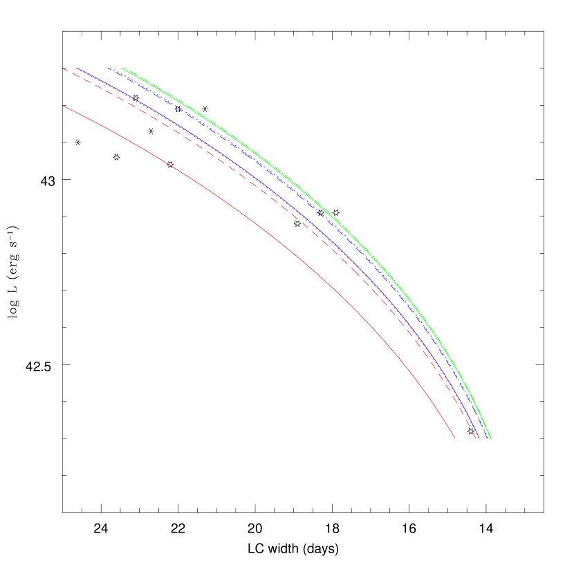
Figure 3: Sensitivity of the bolometric light curve luminosity-width relationship to the initial metallicity. The solid lines belong to Eq. 3 of the present work for $Z=0.1Z_{\odot}$ (green), $Z=Z_{\odot}$ (blue), and $Z=3Z_{\odot}$ (red). There are also shown the curves obtained using the $M(^{56}\mathrm{Ni})$ vs Z relationships of TBT03 (dotted lines) and H09 (dashed lines). The stars represent SNIa from Contardo et al. (2000), whose light-curve width has been computed as in M07, while the asterisks represent SN1999ac (Phillips et al. 2006), SN2003du (Stanishev et al. 2007), and SN2005df (Wang et al. 2009) (by order of decreasing LC width), estimated from the published bolometric light curves

The relationship between $L$ and $\tau$ derived from Eqs. 3, 4 and 5 is displayed in Fig. 3 for three different metallicities along with observational data. There are also represented the relationships obtained by substituting Eq. 3 by the $M(^{56}\mathrm{Ni})$ vs $Z$ dependences proposed by TBT03 and Eq. 5 in H09. Our Eq. 3 gives a wider range of $M(^{56}\mathrm{Ni})$, which accounts better for the scatter of the observational data. Indeed, if real SNIa follow Eq. 3, deriving supernova luminosities from $Z$-uncorrected LC shapes might lead to systematic errors of up to 0.5 magnitudes.

To estimate the bearing that the metallicity dependence of $M(^{56}\mathrm{Ni})$ can have on cosmological studies that use a large observational sample of supernovae, we have generated a virtual population of 200 SNIa that has been analyzed following the same methodology as G08 and H09. Each virtual supernova has been randomly assigned a progenitor metallicity, from a uniform distribution of $\log(Z)$ between $Z_{\mathrm{min}}=0.1Z_{\odot}$ and $Z_{\mathrm{max}}=3Z_{\odot}$, and an $M_{\mathrm{Fe}}$, uniformly distributed in the range from 0.31 to 1.15 $\mathrm{M}_{\odot}$. The minimum and maximum $M(^{56}\mathrm{Ni})$ thus obtained (computed with Eq. 3 and $M_{\mathrm{ec}}=0.14~{}\mathrm{M}_{\odot}$) are $0.1$ and $1~{}\mathrm{M}_{\odot}$, and the bolometric LC width, $\tau$, lies in the range $15-24$ days. A $Z$-uncorrected mass of ⁵⁶Ni, $M^{\odot}_{56}$, has then been obtained as the value of $M(^{56}\mathrm{Ni})$ that would give the same $\tau$ if $Z=Z_{\odot}$. The $M^{\odot}_{56}$ so computed gives an idea of the effect of fitting an observed SNIa LC with a template that takes no account of the supernova metallicity. From Eq. 4, we estimate the Hubble Residual, HR, of each virtual SNIa at: $\mathrm{HR}=2.5\log\left(M^{\odot}_{56}/M(^{56}\mathrm{Ni})\right)$. As a final step we have added gaussian noise with $\sigma=0.1$ to both HR and $\log(Z)$, to simulate the effect of observational uncertainties.

A linear relationship $\mathrm{HR}=\alpha+\beta\log(Z)$ has then been fit to the noisy virtual data by the least-squares technique, as in G08 and H09. Figure 4 shows the results for 10,000 realizations of the noisy virtual dataset. The histogram gives the number counts of the slope $\beta$ in the 10,000 realizations. The whole process has been repeated by using Eq. 2 (i.e. the linear scenario) to represent the dependence of $M(^{56}\mathrm{Ni})$ on $Z$ and the results are also shown in Fig. 4. From the Figure it is clear that, for a large enough set of SNIa whose luminosity and metallicity are measured with small enough errors, it is possible to discriminate between the linear and non-linear scenarios. In our numerical experiment, the mean value of $\beta$ is 0.13 in the first case and 0.26 in the second case, both with a standard deviationof 0.02.

Figure 4 shows also the observational results obtained by G08, who approximated the metallicities of the SNIa in their sample by the $Z$ of the host galaxy, obtained from an empirical galactic mass-metallicity relationship. The striking match between our results based on the non-linear scenario and those of G08 must be viewed with caution in view of the observational uncertainties involved in measuring supernova metallicities and the limitations of our models (i.e. the assumption of spherical symmetry). Recently, using a different method of determination of the SNIa metallicity, H09 arrived to a result opposite to that of G08, i.e. they found that HR is uncorrelated with $Z$, leading to a distribution centered around $\beta\approx 0$. Thus, until such discrepancies are resolved it is not possible to draw any firm conclusion about the metallicity effect on SNIa luminosity. However, it is worth stressing that the simultaneous measurement of supernova luminosity and metallicity for a large SNIa set would strongly constrain the physics of the deflagration-to-detonation transition in thermonuclear supernovae, one of the key standing problems in supernova theory.

Table 1: Properties of CO cores at the beginning of TPs

$Z$	$M_{0}$	$M_{\mathrm{core}}$	$X_{\mathrm{c}}$ (12C)	$\eta_{\mathrm{c}}$	$X_{\mathrm{sim}}$ (12C)	$\eta_{\mathrm{sim}}$
	($\mathrm{M}_{\odot}$)	($\mathrm{M}_{\odot}$)
$10^{-5}$ (0.23)	3	0.801	0.28	$8.7\times 10^{-7}$	0.38	$1.9\times 10^{-3}$
$10^{-5}$ (0.23)	5	0.903	0.25	$8.6\times 10^{-7}$	0.31	$1.7\times 10^{-3}$
$10^{-5}$ (0.23)	6.5	1.052	0.20	$8.4\times 10^{-7}$	0.24	$1.5\times 10^{-3}$
0.014 (0.269)	3	0.615	0.23	$1.2\times 10^{-3}$	0.36	$3.7\times 10^{-3}$
0.014 (0.269)	5	0.848	0.32	$1.2\times 10^{-3}$	0.38	$3.0\times 10^{-3}$
0.014 (0.269)	7	1.005	0.22	$1.2\times 10^{-3}$	0.26	$2.7\times 10^{-3}$
0.040 (0.31)	3	0.608	0.18	$3.4\times 10^{-3}$	0.33	$6.0\times 10^{-3}$
0.040 (0.31)	5	0.843	0.32	$3.4\times 10^{-3}$	0.39	$5.4\times 10^{-3}$
0.040 (0.31)	7	1.032	0.28	$3.4\times 10^{-3}$	0.30	$5.1\times 10^{-3}$
0.10 (0.38)	3	0.624	0.15	$7.3\times 10^{-3}$	0.29	$10.1\times 10^{-3}$
0.10 (0.38)	5	0.846	0.29	$7.6\times 10^{-3}$	0.34	$9.6\times 10^{-3}$
0.10 (0.38)	7	0.962	0.23	$7.6\times 10^{-3}$	0.26	$9.5\times 10^{-3}$

Figure 2: Fraction of Fe-group elements (from Ti to Zn) synthesized in layers experiencing incomplete Si-burning ($T_{\mathrm{max}}\leq 5.2\times 10^{9}$ K) as a function of the total mass of Fe-group elements ejected. The filled square is a reference model with $\rho_{\mathrm{DDT}}=3\times 10^{7}$ g cm^-3, $Z=10^{-5}$, and $M_{0}=5\mathrm{M}_{\odot}$, that accounts for the simmering phase. The empty squares belong to models with varying $\rho_{\mathrm{DDT}}$, from $2.6\times 10^{7}$ to $10^{7}$ g cm^-3. All the above models are linked by a solid line to help guiding the eye. The rest of models show the sensitivity to different model parameters with respect to the reference model, as follows: crosses, varying $Z$; empty circles, varying $M_{0}$; stars, varying $\rho_{\mathrm{c}}$

Figure 4: Number distribution of the slope, $\beta$, of the least-squares fit to the Hubble residual vs metallicity. The statistics used 10,000 data sets, each one obtained adding gaussian noise ($\sigma=0.1$ in HR, and 0.1 dex in $Z$) to a virtual random population of 200 SNIa generated using either the quadratic $M(^{56}\mathrm{Ni})$ vs Z relationship (Eq. 3, horizontally hatched histogram) or the linear relationship (Eq. 2, vertically hatched histogram). The vertical dashed line shows the slope measured by G08

References

- Badenes et al. (2003) Badenes, C., Bravo, E., Borkowski, K. J., & Domínguez, I. 2003, ApJ, 593, 358
- Badenes et al. (2008) Badenes, C., Bravo, E., & Hughes, J. P. 2008, ApJ, 680, L33
- Badenes et al. (2009) Badenes, C., Harris, J., Zaritsky, D., & Prieto, J. L. 2009, ApJ, 700, 727
- Brachwitz et al. (2000) Brachwitz, F., Dean, D. J., Hix, W. R., et al. 2000, ApJ, 536, 934
- Bravo et al. (1992) Bravo, E., Isern, J., Canal, R., & Labay, J. 1992, A&A, 257, 534
- Caughlan et al. (1985) Caughlan, G. R., Fowler, W. A., Harris, M. J., & Zimmerman, B. A. 1985, Atomic Data and Nuclear Data Tables, 32, 197
- Chamulak et al. (2007) Chamulak, D. A., Brown, E. F., & Timmes, F. X. 2007, ApJ, 655, L93
- Chamulak et al. (2008) Chamulak, D. A., Brown, E. F., Timmes, F. X., & Dupczak, K. 2008, ApJ, 677, 160
- Chieffi et al. (1998) Chieffi, A., Limongi, M., & Straniero, O. 1998, ApJ, 502, 737
- Contardo et al. (2000) Contardo, G., Leibundgut, B., & Vacca, W. D. 2000, A&A, 359, 876
- Cooper et al. (2009) Cooper, M. C., Newman, J. A., & Yan, R. 2009, ApJ, 704, 687
- Domínguez et al. (2001) Domínguez, I., Höflich, P., & Straniero, O. 2001, ApJ, 557, 279
- Ellis et al. (2008) Ellis, R. S., Sullivan, M., Nugent, P. E., et al. 2008, ApJ, 674, 51
- Gallagher et al. (2008) Gallagher, J. S., Garnavich, P. M., Caldwell, N., et al. 2008, ApJ, 685, 752
- Hamuy et al. (2000) Hamuy, M., Trager, S. C., Pinto, P. A., et al. 2000, AJ, 120, 1479
- Hix & Thielemann (1996) Hix, W. R. & Thielemann, F. 1996, ApJ, 460, 869
- Howell et al. (2009) Howell, D. A., Sullivan, M., Brown, E. F., et al. 2009, ApJ, 691, 661
- Kasen et al. (2009) Kasen, D., Röpke, F. K., & Woosley, S. E. 2009, Nature, 460, 869
- Khokhlov (1991) Khokhlov, A. M. 1991, A&A, 245, 114
- Kunz et al. (2002) Kunz, R., Fey, M., Jaeger, M., et al. 2002, ApJ, 567, 643
- Lentz et al. (2000) Lentz, E. J., Baron, E., Branch, D., Hauschildt, P. H., & Nugent, P. E. 2000, ApJ, 530, 966
- Lodders (2003) Lodders, K. 2003, ApJ, 591, 1220
- Mazzali et al. (2007) Mazzali, P. A., Röpke, F. K., Benetti, S., & Hillebrandt, W. 2007, Science, 315, 825
- Phillips et al. (2006) Phillips, M. M., Krisciunas, K., Suntzeff, N. B., et al. 2006, AJ, 131, 2615
- Piersanti et al. (2003) Piersanti, L., Gagliardi, S., Iben, I. J., & Tornambé, A. 2003, ApJ, 598, 1229
- Piro & Bildsten (2008) Piro, A. L. & Bildsten, L. 2008, ApJ, 673, 1009
- Röpke & Niemeyer (2007) Röpke, F. K. & Niemeyer, J. C. 2007, A&A, 464, 683
- Stanishev et al. (2007) Stanishev, V., Goobar, A., Benetti, S., et al. 2007, A&A, 469, 645
- Straniero et al. (2003) Straniero, O., Domínguez, I., Imbriani, G., & Piersanti, L. 2003, ApJ, 583, 878
- Taubenberger et al. (2008) Taubenberger, S., Hachinger, S., Pignata, G., et al. 2008, MNRAS, 385, 75
- Timmes et al. (2003) Timmes, F. X., Brown, E. F., & Truran, J. W. 2003, ApJ, 590, L83
- Townsley et al. (2009) Townsley, D. M., Jackson, A. P., Calder, A. C., et al. 2009, ApJ, 701, 1582
- Travaglio et al. (2005) Travaglio, C., Hillebrandt, W., & Reinecke, M. 2005, A&A, 443, 1007
- Umeda et al. (1999) Umeda, H., Nomoto, K., Yamaoka, H., & Wanajo, S. 1999, ApJ, 513, 861
- Wang et al. (2009) Wang, X., Li, W., Filippenko, A. V., et al. 2009, ApJ, 697, 380
- Woosley (2007) Woosley, S. E. 2007, ApJ, 668, 1109
- Yoon & Langer (2004) Yoon, S. & Langer, N. 2004, A&A, 419, 623