Theory of resonant photon drag in monolayer graphene

Abstract

Photon drag current in monolayer graphene with degenerate electron gas is studied under interband excitation near the threshold of fundamental transitions. Two main mechanisms generate an emergence of electron current. Non-resonant drag effect (NDE) results from direct transfer of in-plane photon momentum ${\bf q}$ to electron and dependence of matrix elements of transitions on ${\bf q}$. Resonant drag effect (RDE) originates from ${\bf q}$-dependent selection of transitions due to a sharp form of the Fermi distribution in energy. The drag current essentially depends on the polarization of radiation and, in general, is not parallel to ${\bf q}$. The perpendicular current component appears if the in-plain electric field is tilted towards ${\bf q}$. The RDE has no smallness connected with $q$ and exists in a narrow region of photon frequency $\omega$: $|\hbar\omega-2\epsilon_{F}|<\hbar sq$, where $s$ is the electron velocity.

I Introduction

Though the theoretical study of two-dimensional carbon has a long history wall ,Slon ,divinch ,ando1 only after experimental evidence of existence of graphene as a stable two-dimensional crystal alpha , berg ; geim ; zhang this material became very popular. The presence of zero gap and zero electron mass, combined with a rather high mobility at room temperature, makes graphene an unique material for various fundamental and applied problems. At present graphene is intensively studied both theoretically and experimentally (see e.g. reviews geim2 ; rev4 ).

The study of graphene optics (see alpha3 ,falk ) is stimulated by the prediction that the absorption in monolayer graphene should be determined by the fundamental constant $\alpha=e^{2}/\hbar c$ ando , alpha2 and its experimental evidence nair . The investigation of coupling between photons and electrons in graphene attracts now an active interest of the community (see e.g. ziegler1 ; ziegler2 ). An observation of amplified stimulated terahertz emission from optically pumped epitaxial graphene heterostructures has been reported recently thzgener . However, the photoinduced currents, namely, photon drag and photogalvanic effects in graphene were beyond of interest of the researchers. In this paper we present the theoretical analysis of these effects.

The study of light pressure on solids has rather long history. The simplest variant is an instantaneous transmission of photon momentum to electrons. This process is permitted for interband transitions or in presence of the ”third body”, for example, phonons, other electrons, impurities. For a free particle this process is forbidden by conservation laws. Small value of the photon momentum makes Nonresonant photon Drag Effect (NDE) extremely weak.

At the same time there exists a less known variant of this effect, namely Resonant photon Drag Effect (RDE) which has no weakness of usual NDE grinb ,kast ,alper . Resonance drag occurs when some partial kinetic property of electron gas sharply depends on electron energy. A small photon momentum gives an increase of the electron energy, that can drastically change the relaxation time. This leads to a significantly different contributions to the electron current for electrons exited along or oppositely to the photon direction. In alper the situation was studied for interband transitions in weakly doped GaAs when the electron energy approaches the energy of longitudinal optical phonon. In this case electrons exited along the direction of photon have larger energy than electrons in opposite direction. Hence, their energy can exceed the threshold for emission of optical phonon: they quickly emit phonons and stop, while the opposite electrons will move freely till they collide with impurity. This gives rise to the appearance of charge flow in the direction opposite to the light ray.

Here we develop another idea for RDE based on a sharp Fermi distribution which forbids the transitions below the Fermi energy $\epsilon_{F}$. This idea is illustrated in Fig.1. Electrons are excited from the hole cone to the electron cone by photons with frequency $\omega$ and wave vector ${\bf Q}$. The conditions for resonant transitions are $sk+s|{\bf k-q}|=\omega$, $\hbar s|{\bf k}|>\epsilon_{F}$, where ${\bf k}$ is the electron momentum counted from the cone point, $s\approx 10^{8}$cm/s is the electron velocity, and ${\bf q}$ is a projection of the wave vector ${\bf Q}$ of radiation to the plane of graphene. The first condition determines ellipse in ${\bf k}$ plane, the second limits a part of this ellipse accessible for transitions. The wave vector tilts the transitions towards its direction. Fig. 1 shows the case when the frequency is close to $2\epsilon_{F}$. The electrons in the figure are excited from the right segment of the Fermi surface contour. This results in electron flow rightwards. Since $q\ll k_{F}$ the RDE appears when the frequency is close to $2\epsilon_{F}$, namely if $|\omega-2\epsilon_{F}|<sq$. Inside this window the current of RDE has no smallness connected with $q$ and can be estimated as $j\sim es\tau~{}\pi\alpha~{}P/(\hbar\omega)$, where $e$ and $s$ are the electron charge and the velocity, $\pi\alpha$ is the opacity of graphene, $\tau$ is the transport relaxation time and $P$ is the light intensity. Physical meaning of this estimation is evident: $\tau\pi\alpha P/(\hbar\omega)$ is the instantaneous density of exited electrons which conserve their momentum. Being multiplied by the current of individual electrons $es$, this quantity gives the current density.

Below we determine both NDE and RDE for interband transitions in monolayer graphene with degenerate electron gas. Due to graphene electron-hole symmetry results are applicable to n- and p-type graphene. In general the relaxation process for electrons and holes are different that breaks electron-hole symmetry. For concreteness, we consider the n-type graphene. In this case the mean free time of excited electrons is much longer than that of holes since due to different distance from the Fermi level holes can easier emit phonons. Thus, the contribution of holes will be neglected.

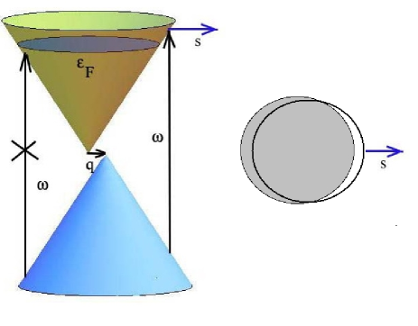
Figure 1: (Color online) Interband phototransitions in n-type graphene. Left panel: diagram of transitions in the momentum-energy space. The hole cone is shifted in $\bf k$ space by the photon wave vector $\bf q$. The transitions are permitted only above the Fermi level. Right panel: projection to the momentum plane. Filled circle represents the Fermi sea, the elliptic curve corresponds to the energy conservation equation $s|{\bf k-q}|+sk=\omega$; only momenta outside the Fermi circle are permitted corresponding to the right segment of the elliptic curve.

Fig. 2 illustrates a possible experiment on excitation of the drag current in a suspended graphene sheet placed in $(x,y)$ plane. Light with frequency $\omega$, wave vector $\bf Q$ ($Q=\omega/c$) and amplitude of electric field $\cal E$ illuminates graphene plane. We consider transitions near the cone singularity. In this case the current is determined by the projections of the electric field and the wave vector onto the graphene layer. These quantities are ${\bf E}\equiv{\bf e}E=({\cal E}_{p}\cos\beta,{\cal E}_{s})$ and ${\bf q}=(1,0)Q\sin\beta$, where $\beta$ is the angle of incidence, ${\cal E}_{s}$ and ${\cal E}_{p}$ are amplitude components of the electric field $\cal E$ perpendicular and parallel to the incident plane. We ignore small modification of field caused by the layer.

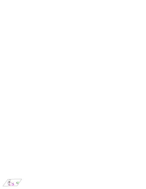
Figure 2: (Color online) Sketch of proposed experiment (see text for details).

II Basic equations

The current of photon drag effect can be expressed via the probability of transition $g({\bf k})$ from the hole state with a momentum ${\bf k-q}$ to the electron state with momentum ${\bf k}$ and the electron velocity ${\bf v}({\bf k})=s{\bf k}/k$ as

$${\bf j}=4e\int\frac{d{\bf k}}{4\pi^{2}}{\bf v}({\bf k})\tau g({\bf k}),$$ (1)

where the coefficient 4 accounts for the valley and spin degeneracies. The dependence on the photon momentum results from the momentum and energy conservation laws and the matrix elements for transition. For simplicity we put below $\hbar=1$.

The two-band Hamiltonian near the Dirac point is

$$\hat{H}({\bf k})=s\left(\begin{array}[]{cc}0&k_{x}-ik_{y}\\ k_{x}+ik_{y}&0\\ \end{array}\right)=s{\bf k}\mbox{\boldmath{$\sigma$}}.$$ (4)

Here $\sigma$ is the vector of the Pauli matrices. The eigenvalues and eigenvectors of the Hamiltonian (4) are $\epsilon_{\pm}({\bf k})=\pm sk$ and $\Psi_{\pm}({\bf k})=(1,\pm e^{i\phi_{\bf k}})/\sqrt{2}$, where $\phi_{\bf k}$ is the polar angle of the vector ${\bf k}$. The different signs correspond to electrons and holes. The interaction with the wave is determined by the matrix elements of the velocity $\nabla_{\bf k}\hat{H}({\bf k})=s\mbox{\boldmath{$\sigma$}}$ between the hole and electron states with the momenta ${\bf k-q}$ and ${\bf k}$: ${\bf v}^{-+}=(\Psi_{-}({\bf k-q})^{*}s\mbox{\boldmath{$\sigma$}}\Psi_{+}({\bf k}))$, correspondingly.

The transition probability $g({\bf k})$ is

$$g({\bf k})=\frac{\pi e^{2}}{2\omega^{2}}|{\bf E}{\bf v}^{+-}|^{2}\delta(sk+s|{\bf k}-{\bf q}|-\omega)\theta(\epsilon_{\bf k}-\epsilon_{F}),$$ (5)

where $\theta(t)$ is the Heaviside function. The expression for current Eq.(1) can be rewritten as

$${\bf j}=\frac{e^{3}E^{2}s^{3}}{2\pi\omega^{2}}\int d{\bf k}\tau\frac{\bf k}{|{\bf k}|}a_{jk}e_{j}e_{k}\delta(sk+s|{\bf k-q}|-\omega)\theta(sk-\epsilon_{F})$$ (6)

where

$$a_{jk}=\frac{1}{s^{2}}v_{j}^{-+*}v_{k}^{-+}.$$ (7)

We utilized the symmetry of the tensor $a_{ij}$ resulting to inclusion of the field polarization in the combinations $e_{i}^{*}e_{j}+e_{j}^{*}e_{i}$ only and independence on the degree of circular polarization. Hence, without loss of generality one can consider the field as linear-polarized and ${\bf e}$ as real.

Due to the smallness of the wave vector $q$, as compared to the electron momentum, one can expand all quantities in powers of $q$. Expanding by $q$ we can write the argument of the delta-function as $sk+s|{\bf k}-{\bf q}|-\omega\approx 2sk-\omega-sq\cos\phi_{\bf k}$ (we choose the direction of axis x along ${\bf q}$). At the same time, $q$ is comparable with $2sk-\omega$ and we keep ourselves from subsequent expansion of the delta-function.

Expanding the tensor $a_{ij}$, we have

$$a_{xx} = \sin^{2}\phi_{\bf k}(1+\frac{q}{k}\cos\phi_{\bf k}),$$

$$a_{yy} = \cos^{2}\phi_{\bf k}-\frac{q}{k}\sin^{2}\phi_{\bf k}\cos\phi_{\bf k},$$ (8)

$$2\mbox{Re}(a_{xy}) = -2\sin\phi_{\bf k}\cos\phi_{\bf k}-\frac{q}{k}\sin\phi_{\bf k}\cos(2\phi_{\bf k})$$

From Eq.(6) we obtain for components of the current

$$j_{x}=-2J_{0}\int_{-1}^{min(1,a)}\frac{dx}{\sqrt{1-x^{2}}}\frac{\tau}{\tau_{0}}\times~{}~{}~{}~{}~{}~{}~{}~{}~{}~{}~{}~{}~{}~{}~{}~{}~{}$$

$$\Big{\{}e_{x}^{2}[-x(1-x^{2})(1+bx)+2b(1-x^{2})(1-2x^{2})]+$$

$$e_{y}^{2}[-x^{3}(1+bx)+4bx^{2}(1-x^{2})]\Big{\}};$$ (9)

$$j_{y}=2J_{0}e_{x}e_{y}\int_{-1}^{min(1,a)}dx\frac{\tau}{\tau_{0}}\sqrt{1-x^{2}}\times~{}~{}~{}~{}~{}~{}~{}~{}~{}$$

$$\Big{\{}-2x(1-x^{2})(1+bx)+2b(3x^{2}-1)\Big{\}}.$$ (10)

Here we have introduced the following notations:

$$J_{0}=\frac{e^{2}}{\hbar c}\frac{cE^{2}}{8\pi\hbar\omega}|e|\tau_{0}s,~{}~{}\tau_{0}=\tau|_{k=k_{F}},~{}~{}a=\frac{\omega-2\epsilon_{F}}{sq},~{}~{}b=\frac{sq}{\omega}.$$

If $\tau$ is independent on the energy of electrons then the integration in Eq.(II) can be done directly. The current has different values inside and outside the region $|\omega-2\epsilon_{F}|<sq$. If $|\omega-2\epsilon_{F}|<sq$ then we have

$$j_{x} = -\frac{2}{3}J_{0}\sqrt{1-a^{2}}((1-a^{2})e_{x}^{2}+(2+a^{2})e_{y}^{2}),$$ (11)

$$j_{y} = -\frac{4}{3}J_{0}(1-a^{2})^{3/2}e_{x}e_{y}.$$ (12)

These values represent resonant photon drag RDE. It remains constant if $q\to 0$. The value of resonant current is determined by $J_{0}$. For the photon flow $cE^{2}/8\pi\hbar\omega=10^{19}$cm^-2s^-1, $\tau=10^{-12}$ s, $J_{0}=1.16\cdot 10^{-6}$A/cm. This approximately corresponds to a power of $0.1W/cm^{2}$ for photons with energy $0.1eV$.

If $|\omega-2\epsilon_{F}|>sq$, then there is only NDE current. It is proportional to $q$:

$$j_{x} = J_{0}\frac{\pi sq}{4\omega}(3e_{x}^{2}-e_{y}^{2}),$$ (13)

$$j_{y} = \frac{3}{2}J_{0}\frac{\pi sq}{\omega}e_{x}e_{y}.$$ (14)

The value of NDE is significantly smaller then the RDE value.

In agreement with the simple estimates the RDE has always the direction opposite to the direction of light wave vector. Its polarization dependence is explained by the dependence of the directional diagram of excitation: most of carriers are excited perpendicular to the polarization. At the same time the Fermi sea limits the transitions by the direction of the photon wave vector. This circumstances together determine lower x-component of current if ${\bf e}||{\bf q}$ in comparison with the case ${\bf e}\perp{\bf q}$ and also the appearance of y-component of the RDE current.

In agreement with the system symmetry, $j_{y}$ exists only if the polarization has both $e_{x}$ and $e_{y}$ components. The RDE current exists in a narrow window $|\omega-2\epsilon_{F}|<sq$ which shrinks if $q\to 0$. But inside this window RDE is much stronger than NDE so the later can be neglected in this window.

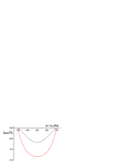
Figure 3: Resonant photon drag current in units of $J_{0}$ versus normalized frequency $(\omega-2\epsilon_{F})/sq$. The solid curve shows the longitudinal component of current $j_{x}$, the field is polarized along the projection of the wave vector on the plane ($\theta=0$) and $j_{y}$ at $\theta=\pi/4$. The dashed curve shows $j_{x}$ at $\theta=\pi/2$.

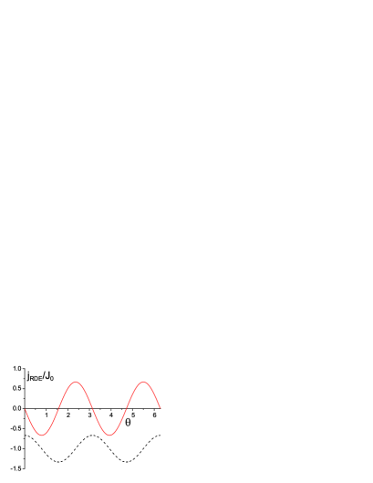
Figure 4: Polarization dependence of the RDE current at $\omega=2\epsilon_{F}$; $j_{x}$ is shown by dash curve, $j_{y}$ is shown by solid curve.

The sign of x-component of NDE depends on polarization. This contradicts to a simple assumption according to which the current is mainly determined by kicks which photons give to electrons. The origin of this difference is the dependence of the directional diagram on the small wave vector ${\bf q}$ via the parameter $a_{ij}$: at some polarizations electrons prefer to be excited in opposite direction to ${\bf q}$. This explains the change of sign.

Fig. 3 demonstrates the dependence of RDE current components on the frequency in the window $|\omega-2\epsilon_{F}|<sq$ where RDE exists. The current vanishes at the edges of the window. The component $j_{x}$ is larger for the polarization along the y axis. The component $j_{y}$ appears only for tilted polarization of the light. Fig. 4 shows the dependence of $j_{x}$ and $j_{y}$ on the angle $\theta$ between the vector of polarization ${\bf e}$ and the wave vector ${\bf q}$.

III Discussion

We have studied the electron contribution to the photon drag current. In fact, in the considered system the hole contribution also presents. The symmetry between holes and electrons in a neutral system means that these contributions double. However, the result will be changed if to take into account the difference between electrons and holes caused by their different excitation energy: while electrons are generated near the Fermi energy the holes appear well below the Fermi energy. This leads to a strong difference between the relaxation times. In high-mobility samples at low temperature the momentum relaxation time near the Fermi energy is much greater than far from the Fermi energy. At the same time, quick relaxation of excited electrons (holes) to the Fermi energy due to electron-electron interaction (described by e-e relaxation time $\tau_{ee}$) conserves their momenta up to the moment when excitations reaches the temperature layer. This results in equality of holes and electrons contributions to the current. And vice versa, electron-phonon relaxation can cancel the hole contribution if $\tau_{e-ph}\ll\tau_{ee}$, where $\tau_{e-ph}$ is the time of energy relaxation due to electron-phonon collisions. Thus, the obtained current should be multiplied by a factor 2 in the case of quick e-e relaxation and be kept unchanged in the opposite case. We note, that when the Fermi energy tends to zero the system becomes symmetric.

The RDE exists in a narrow energy range $\Delta\epsilon\approx\hbar sq\approx\hbar\omega s/c$ near the Fermi energy. This means that the RDE is visible for temperature $T<\Delta\epsilon$. For photons with $\hbar\omega=0.1eV$ this gives $T<3K$.

The observation of the resonant photon drag in monolayer graphene is accessible to the modern experimental technique that allows to investigate interesting aspects of coupling between photons and electrons in this material.

IV Acknowledgments

We thank A.D.Chepelianskii for useful discussions. The work was supported by grant of RFBR No 08-02-00506 and No 08-02-00152 and ANR France PNANO grant NANOTERRA; MVE and LIM thank Laboratoire de Physique Théorique, CNRS for hospitality during the period of this work.

References

- (1) P.R. Wallace, Phys. Rev. 71, (1947) 622;
- (2) J.C. Slonczewski and P.R. Weiss, Phys. Rev. 109, (1958) 272.
- (3) D.P. DiVincenzo and E.J. Mele, Phys. Rev. B 29, (1984) 1685.
- (4) T. Ando, T. Nakanishi, and R. Saito, J. Phys. Soc. Japan 67, (1998) 2857.
- (5) K.S. Novoselov, A.K. Geim, S.V. Morozov, D. Jiang, Y. Zhang, S.V. Dubonos, I.V. Grigorieva, and A.A. Firsov, Science, 306, 666 (2004).
- (6) C. Berger, Z. Song, X. Li, X. Wu, N. Brown, C. Naud, D. Mayou, T. Li, J. Hass, A.N. Marchenkov, E.H. Conrad, P.N. First, and W.A. de Heer, Science 312, 1191 (2006).
- (7) K. S. Novoselov, A.K. Geim, S.V. Morozov, D. Jiang, M.I. Katsnelson, I.V. Grigorieva, S.V. Dubonos, A.A. Firsov , Nature 438, 197 (2005).
- (8) Y. Zhang, J.W. Tan, H.L. Stormer, and P. Kim, Nature 438, 201 (2005).
- (9) A.K. Geim and K.S. Novoselov, Nature Materials 6, 183 (2007).
- (10) A.H. Castro Neto, F. Guinea, N.M.R. Peres, K.S. Novoselov, and A.K. Geim, Rev. Mod. Phys., 81, 109 (2009).
- (11) L.A. Falkovsky and A.A. Varlamov, Eur. Phys. J. B, 56, 281 (2007).
- (12) L.A. Falkovsky, Phys. Usp. 51, 887 (2008) [Usp. Fiz. Nauk,178, 923 (2008)]
- (13) T. Ando, Y. Zheng and H. Suzuura, J. Phys. Soc. Japan, 71, 1318 (2002).
- (14) V.P. Gusynin, S.G. Sharapov and J.P. Carbotte, Phys. Rev. Lett. 96, 256802 (2006).
- (15) R.R.Nair, P.Blake, A.N.Grigorenko, K.S.Novoselov, T.J.Booth, T.Stauber, N.M.R.Peres, A. K. Geim, Science, 320, 1308 (2008).
- (16) J.Z. Bernád, U.Zülicke, and K. Ziegler, arXiv:1001.3239[cond-mat] (2010).
- (17) K. Ziegler and A. Sinner, arXiv:1001.3366[cond-mat] (2010).
- (18) T.Otsuji, H.Karasawa, T.Komori, T.Watanabe, H.Fukidome, M.Suemitsu, A.Satou, and Victor Ryzhii, arXiv:1001.5075[cond-mat] (2010).
- (19) A. A. Grinberg, Zh. Eksp. Teor. Fiz. 58, 989 (1970) [Sov. Phys.-JETP 31, 531 (1970)].
- (20) A.M.Danishevskii, A.A.Kastal’skii, S.M.Ryvkin, and I.D.Yaroshetskii, Zh.Exp.Teor.Fiz. 58, 544 (1970) [Sov. Phys. JETP, 31, 292 (1970)].
- (21) V.L. Al’perovich, V.I. Belinicher, V.N. Novikov, and A.S. Terekhov, 33, 557 (1981) [Sov. Phys.-JETP Lett., 33, 573 (1981)].