AAOmega Observations of 47 Tucanae:
Evidence for a Past Merger?

Abstract

The globular cluster 47 Tucanae is well studied but it has many characteristics that are unexplained, including a significant rise in the velocity dispersion profile at large radii, indicating the exciting possibility of two distinct kinematic populations. In this Letter we employ a Bayesian approach to the analysis of the largest available spectral dataset of 47 Tucanae to determine whether this apparently two-component population is real. Assuming the two models were equally likely before taking the data into account, we find that the evidence favours the two-component population model by a factor of $\sim 3\times 10^{7}$. Several possible explanations for this result are explored, namely the evaporation of low-mass stars, a hierarchical merger, extant remnants of two initially segregated populations, and multiple star formation epochs. We find the most compelling explanation for the two-component velocity distribution is that 47 Tuc formed as two separate populations arising from the same proto-cluster cloud which merged $\lesssim 7.3\pm 1.5$ Gyr ago. This may also explain the extreme rotation, low mass-to-light ratio and mixed stellar populations of this cluster.

1 Introduction

As one of the closest and most massive Galactic globular clusters (GCs), 47 Tucanae (catalog 47 Tuc) (47 Tuc) is a test-bed for Galaxy formation models (Salaris et al., 2007, and references therein), distance measurement techniques (e.g. Bono et al., 2008) and metallicity calibrations (e.g. McWilliam & Bernstein, 2008; Lane et al., 2009b). This close examination, however, has left several unresolved conundrums. While not unique in this respect (see Gratton et al., 2004, for a review of elemental abundance variations in GCs), 47 Tuc has a bimodal distribution of carbon and nitrogen line strengths (e.g. Harbeck et al., 2003). Furthermore, 47 Tuc has a complex stellar population, exhibiting, for example, multiple sub-giant branches (e.g. Anderson et al., 2009). Although multiple Red Giant and Horizontal Branches can also be found in other GCs, and may be due to chemical anomalies (e.g. Ferraro et al., 2009; Lee et al., 2009), 47 Tuc is particularly unusual in many respects. It has an extreme rotational velocity (a property it shares only with M22 and $\omega$ Centauri, e.g. Merritt et al., 1997; Anderson & King, 2003; Lane et al., 2009b) and an apparently unique rise in its velocity dispersion profile at large radii Lane et al. (2009b).

Furthermore, the mass-to-light ratio (M/L_V) of 47 Tuc is very low for its mass Lane et al. (2010), that is, it does not obey the mass-M/L_V relation described by Rejkuba et al. (2007). Note that this mass-M/L_V relation is not due to the presence of dark matter but because of dynamical effects Kruijssen (2008). Explanations for these unusual properties may be intimately linked to its evolutionary history. In this Letter we describe and analyse various explanations for the rise in velocity dispersion in the outer regions of 47 Tuc initially reported by Lane et al. (2009b).

Lane et al. (2009b) provided a complete description of the data acquisition and reduction, radial velocity uncertainty estimates, the membership selection process, and statistical analysis of cluster membership for all data presented in this Letter.

2 Plummer Model Fits

The Plummer (1911) model (see also Dejonghe, 1987) predicts that the isotropic, projected velocity dispersion $\sigma$ falls off with radius $r$ as:

$$\sigma(r;\left\{\sigma_{0},r_{0}\right\})=\frac{\sigma_{0}}{\left(1+\left(\frac{r}{r_{0}}\right)\right)^{1/4}},$$ (1)

where $\sigma_{0}$ is the central velocity dispersion and $r_{0}$ is the scale radius of the cluster. We now describe how we fitted Plummer profiles to the 47 Tuc radial velocity data to infer the values of the parameters $\sigma_{0}$ and $r_{0}$, and also to evaluate the overall appropriateness of the Plummer hypothesis ($H_{1}$) by comparing it to a more complex double Plummer model ($H_{2}$).

The mechanism for carrying out this comparison is Bayesian model selection (Sivia & Skilling, 2006). Suppose we have two (or more) competing hypotheses, $H_{1}$ and $H_{2}$, with each possibly containing different parameters $\theta_{1}$ and $\theta_{2}$. We wish to judge the plausibility of these two hypotheses in the light of some data $D$, and some prior information. Bayes’ rule provides the means to update our plausibilities of these two models, to take into account the data $D$:

$$\frac{P(H_{2}|D)}{P(H_{1}|D)}=\frac{P(H_{2})}{P(H_{1})}\frac{P(D|H_{2})}{P(D|H_{1})}$$

$$=\frac{P(H_{2})}{P(H_{1})}\times\frac{\int_{\theta_{1}}p(\theta_{1}|H_{1})p(D|\theta_{1},H_{1})\,d\theta_{1}}{\int_{\theta_{2}}p(\theta_{2}|H_{2})p(D|\theta_{2},H_{2})\,d\theta_{2}}.$$ (2)

Thus, the ratio of the posterior probabilities for the two models depends on the ratio of the prior probabilities and the ratio of the evidence values. The latter measure how well the models predict the observed data, not just at the best-fit values of the parameters, but averaged over all plausible values of the parameters. It should be noted that we rely solely on the velocity information for our Plummer model fits. Taking the stellar density as a function of radius into account would be useful in further constraining the models. However, the Plummer model fits by Lane et al. (in prep.) based exclusively on velocity information are also good fits to the surface brightness profiles of the four GCs analysed in that study.

2.1 Single Plummer Model

The data are a vector of radial velocity measurements $\mathbf{v}=\{v_{1},v_{2},...,v_{N}\}$ of $N$ stars, along with the corresponding distances from the cluster centre $\mathbf{r}=\{r_{1},r_{2},...,r_{N}\}$ and observational uncertainties on the velocities $\mathbf{\sigma_{\textnormal{obs}}}=\{\sigma_{\textnormal{obs},1},...,\sigma_{\textnormal{obs},N}\}$. We will consider $\mathbf{v}$ to be the data, whereas $\mathbf{r}$ and $\mathbf{\sigma_{\textnormal{obs}}}$ are considered part of the prior information. In this case the probability distribution for the data given the parameters is the product of independent Gaussians, whose standard deviations vary with radius:

$$p(\mathbf{v}|\mu,\sigma_{0}, r_{0})=$$

$$\prod_{i=1}^{N} \left(\frac{1}{\sqrt{2\pi\sigma_{i}^{2}}}\exp\left(-\frac{1}{2}\left(\frac{v_{i}-\mu}{\sigma_{i}}\right)^{2}\right)\right),$$ (3)

where $\mu$ is the systemic velocity of the cluster. The standard deviation $\sigma_{i}$ for each data point is given by a combination of the standard deviation predicted by the Plummer model, and the observational uncertainty:

$$\sigma_{i}=\sqrt{\sigma(r_{i};\left\{\sigma_{0},r_{0}\right\})^{2}+\sigma_{\textnormal{obs},i}^{2}}$$ (4)

To carry out Bayesian Inference, prior distributions for the parameters must also be defined. We assigned a uniform prior for $\mu$ (between $-30$ and 30 km s^-1). For $\sigma_{0}$, we assigned Jeffreys’ scale-invariant prior $p(\sigma_{0})\propto 1/\sigma_{0}$ for $\sigma_{0}$ in the range $0.1-100\textnormal{ km s}^{-1}$. Finally, $r_{0}$ was assigned the Jeffreys’ prior $p(r_{0})\propto 1/r_{0}$ for $r_{0}$ in the range $0.2-220$ pc. These three prior distributions were all chosen to be independent and to cover the approximate range of values that we expect the parameters to take.

2.2 Double Plummer Model

The double Plummer model is a simple extension of the Plummer model. The stars are hypothesised to come from two distinct populations, each having its own Plummer profile parameters (but with a common systemic velocity $\mu$). Thus, at any radius $r$ from the cluster centre, we model the velocity distribution as a mixture (weighted sum) of two Gaussians. From previous work Lane et al. (2009b) we also expect the inner regions of the cluster to be well fitted by a single Plummer profile, so the weight of the second population of stars should become more significant at larger radii.

Thus, instead of having a single $\sigma_{0}$ parameter and a single $r_{0}$ parameter, there are now two of each. The probability distribution for the data given the parameters is then the weighted sum of two Gaussians:

$$p(\mathbf{v}|\mu ,\{\sigma_{0}\},\{r_{0}\},w(r))=$$

$$\prod_{i=1}^{N}\left(\frac{w(r_{i})}{\sqrt{2\pi\sigma_{i,1}^{2}}}\exp\left(-\frac{1}{2}\left(\frac{v_{i}-\mu}{\sigma_{i,1}}\right)^{2}\right)\right.$$

$$+\left.\frac{1-w(r_{i})}{\sqrt{2\pi\sigma_{i,2}^{2}}}\exp\left(-\frac{1}{2}\left(\frac{v_{i}-\mu}{\sigma_{i,2}}\right)^{2}\right)\right).$$ (5)

Here, $w(r)$ is a weight function that determines the relative strength of one Plummer profile with respect to the other, as a function of radius. We expect one component to dominate at smaller radii, and to eventually fade away as the second component becomes dominant. Hence, we parameterise the function $w(r)$ as:

$$w(r)=\frac{\exp\left(u(r)\right)}{1+\exp\left(u(r)\right)}$$ (6)

where

$$u(r)=u_{\alpha}+\frac{r-r_{\textnormal{min}}}{r_{\textnormal{max}}-r_{\textnormal{min}}}\left(u_{\beta}-u_{\alpha}\right).$$ (7)

That is, the log of the relative weight between one Plummer component and the other increases linearly over the range of radii spanned by the data, starting at $u_{\alpha}$ and ending at a value $u_{\beta}$. Parameterising $w$ via $u$ makes it easier to enforce the condition that $w(r)$ must be in the range $0-1$ for all $r$. The prior distributions for $u_{\alpha}$ and $u_{\beta}$ were chosen to be Gaussian with mean zero and standard deviation 3. This implies that $w(r)$ will probably lie between 0.05 and 0.95, with a small but not negligible chance of extending lower than 0.001 or above 0.999.

The standard deviations of the two Gaussians at each data point are given by a combination of that predicted by the Plummer model and the observational uncertainty:

$$\sigma_{i,1} = \sqrt{\sigma(r_{i};\{\sigma_{0},r_{0}\}_{1})^{2}+\sigma_{\textnormal{obs},i}^{2}}$$ (8)

$$\sigma_{i,2} = \sqrt{\sigma(r_{i};\{\sigma_{0},r_{0}\}_{2})^{2}+\sigma_{\textnormal{obs},i}^{2}}$$ (9)

The priors for all the parameters $\mu$, $\{\sigma_{0},r_{0}\}$ were chosen to be the same as in the single Plummer case.

3 Results

An obvious rise in the velocity dispersion of 47 Tuc was described by Lane et al. (2009b, their Figure 11) at approximately half the tidal radius ($\sim 28$ pc). The tidal radius is $\sim 56$ pc Harris (1996). To confirm the reality of this rise, several tests were performed, including resizing the bins and shifting the bin centres, as described by Lane et al. (2009b). No difference in the overall shape of the dispersion profile was found during any tests.

We used a variant Brewer et al. (2009) of Nested Sampling (Skilling, 2006) to sample the posterior distributions for the parameters, and to calculate the evidence values for the single and double Plummer models. The results are listed in Table 1. The double Plummer model is favoured by a factor $\sim 3\times 10^{7}$, and consists of a dominant Plummer profile that fits the inner parts of the radial velocity data (Figure 1), and a second, wider profile that models the stars at large radius.

As a test of the veracity of our model we altered the model so that $w$($r$) was linear (with endpoints in the range $0-1$ and with a uniform prior) rather than $u$($r$) being linear. This had the effect of reducing the log evidence to $\approx-7748$, so in this case the double Plummer model is favoured by a factor $\sim 10^{5}$. This best-fit model has a more subtle increase in width at large radii, when compared with Figure 1. Presumably this is because $w$($r$) being linear prevents more rapid fade-outs. Correspondingly, the Plummer profile represented by the thin curve in Figure 2 was shifted slightly lower. Note that the model in Figure 1 is narrower than the spread of the data, because the spread also arises partly from observational errors. The most extreme points at large radii are likely to be those for which the intrinsic velocity dispersion is large and the observational errors have pushed the points further away from the mean. In Figure 2, the Plummer profiles of the two population components are shown. The inner component is a good fit to the binned velocity dispersions by Lane et al. (2009b). We now discuss possible explanations for this two-component population, and calculate an upper limit on when the second component was introduced.

Table 1: Inferred parameter values for the single Plummer and the double Plummer fits to the 47 Tuc data. The values quoted are the posterior mean $\pm$ the posterior standard deviation, when the marginal posterior distributions were sufficiently symmetric for this to be a reasonable summary. For the few parameters with asymmetric posterior distributions, we instead give the symmetric 68% credible interval. The evidence values imply that if the two models were equally likely before taking into account the data, the data makes the double Plummer model more likely by a factor of $e^{17.3}\approx 3\times 10^{7}$. For the double Plummer model, the first value listed is for the component that dominates at $r=0$.

Parameter	Value
Single Plummer Profile
$\mu$	-16.87 $\pm$ 0.17 km s-1
$\sigma_{0}$	9.37 $\pm$ 0.32 km s-1
$r_{0}$	9.27 $\pm$ 0.98 pc
log(evidence)	-7759.5
Double Plummer Profile
$\mu$	-16.94 $\pm$ 0.12 km s-1
$\sigma_{0}$	9.93 $\pm$ 0.43 km s-1
	[5.70, 13.51] $\pm$ km s-1
$r_{0}$	6.76 $\pm$ 0.94 pc
	[53.6, 4560] pc
$u_{\alpha}$	6.30 $\pm$ 1.30
$u_{\beta}$	-2.30 $\pm$ 1.12
log(evidence)	-7742.2

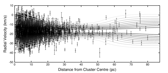
Figure 1: The radial velocities of stars in 47 Tuc together with the best fit double Plummer model for the velocity distribution as a function of radius. The inner part of the cluster is well modelled by the dominant Plummer profile, while at larger radii, the second plummer profile dominates. The radius at which the two profiles have equal weight is 55 pc.

Figure 2: Binned velocity dispersion as a function of radius (from Lane et al., 2009b), with the radial velocity profiles of the two stellar populations from the best fit double Plummer model. The Plummer profile that dominates at small radii is shown as the thick black curve, while the thin curve shows the Plummer profile for the stellar population that dominates at large radii.

3.1 Evaporation

Drukier et al. (2007) carried out $N$-body simulations of GCs through core-collapse and into post-core-collapse. They showed that the evaporation of low-mass stars due to two-body interactions during these phases alters the velocity dispersion profiles in predictable ways. At approximately half the tidal radius ($r_{t}/2$) the velocity dispersion reaches a minimum of $\sim 40$% of the central dispersion, then rises to $\sim 60$% of the central level at $r_{t}$. These criteria are certainly met within 47 Tuc (again, see Figure 11 of Lane et al., 2009b). Furthermore, Lane et al. (2009b) conclude that the rise in velocity dispersion could be explained by evaporation due to the core collapsing, and the Fokker-Planck models by Behler et al. (2003) show that 47 Tuc is nearing core-collapse.

This appears to be reasonable evidence that 47 Tuc is evaporating. However, based on the conclusions drawn by Drukier et al. (2007) and Lane et al. (2010), it is unclear how much Galactic tidal fields affect the outer regions of Galactic globular clusters, and what effect this has on the external velocity dispersion profile. While our best-fit double Plummer model matches the overall form of the trend shown by Drukier et al. (2007) reasonably well (see Figure 1), this scenario does not explain its multiple stellar populations (although these might be explained by chemical anomalies, e.g. Piotto et al., 2007, and references therein), nor its low M/L_V in comparison with its mass (see Figure 6 of Lane et al., 2010), or its extreme rotation. In addition, the extra-tidal stars are spread uniformly across all regions of the colour magnitude diagram (see Figure 3 of Lane et al., 2009b), which is inconsistent with the the two-component population being a consequence of evaporating low-mass stars. We cannot, however, completely discount evaporation without detailed chemical abundance information.

3.2 Merger

Another scenario, which appears to explain most of the unusual properties of 47 Tuc, is that it has undergone a merger in its past (note that this is not the first evidence for such a merger within Galactic GCs, see Ferraro et al., 2002). Several observed quantities can be explained by this hypothesis: (1) the bimodality of the carbon and nitrogen line strengths, (2) the mixed stellar populations, (3) the large rotational velocity, (4) the low M/L_V compared with total mass and (5) the increase in velocity dispersion in the outskirts of the cluster.

In addition to our evidence for two kinematically distinct stellar populations, Anderson et al. (2009) showed that 47 Tuc also has two distinct sub-giant branches, one of which is much broader than the other, as well as a broad main sequence. The authors determined that this broadening may be due to a combination of metallicities and ages, and it is known from previous studies (e.g. Harbeck et al., 2003) that 47 Tuc has a bimodality in its carbon and nitrogen line strengths. While this bimodality is not unique, a merger could explain its origin. Therefore, another possible scenario, which explains many of the properties of 47 Tuc, is a past merger event.

While it might seem unlikely that this is the remnant of a merger, extant kinematic signatures of subgalactic scale hierarchical merging do exist (e.g. within $\omega$ Centauri; Ferraro et al., 2002), and there have been hints that the distinct photometric populations in 47 Tuc might be remnants of a past merger (e.g. Anderson et al., 2009). A possible explanation for this merger hypothesis is given in Section 3.3.

3.3 Initial Formation

The two components may have formed at the same epoch, and the distinct kinematic populations are, therefore, extant remnants from the formation of the cluster itself. If GCs form from a single cloud (see Kalirai & Richer, 2009, for a discussion of GCs as simple stellar populations), it is possible for the proto-cluster cloud to initially contain two overdensities undergoing star formation independently at almost the same time. In this case, the two proto-clusters, which would inevitably be in mutual orbit due to the initially bound nature of the proto-cluster cloud, eventually coalesced through the loss of angular momentum due to dynamical friction.

Note that this scenario is similar to the capture of a satellite described by Ferraro et al. (2002) to explain the merger hypothesis for $\omega$ Centauri, and explains the two kinematic and photometric populations, and the high rotation rate assuming the proto-cluster cloud initially had a large angular momentum. It might also explain the low ${\rm M/L_{V}}$ of this cluster.

Interestingly, Vesperini et al. (2009) show that clusters with initially segregated masses evolve more slowly than non-segregated clusters, having looser cores and reaching core-collapse much later. Because the core of 47 Tuc is highly concentrated and near core-collapse (e.g. Behler et al., 2003) it must be very old if it was initially mass-segregated. 47 Tuc is thought to be 11–14 Gyr old (e.g. Gratton et al., 2003; Kaluzny et al., 2007), hence initial mass segregation is plausible. However, even if 47 Tuc is $\sim 11$ Gyr old the original populations would be kinematically indistinguishable at the present epoch (Section 3.5) indicating that some other process was the cause of the two extant populations described in this Letter. Furthermore, Milky Way GC formation ended about 10.8 Gyr ago (e.g. Gratton et al., 2003), long before the upper limit for the initial mixing of the two populations derived in Section 3.5.

3.4 Multiple Star Formation Epochs

Two star formation epochs in GCs result in the radial separation of the two populations, with the second generation initially concentrated in the core (e.g. D’Ercole et al., 2008, and references therein). Furthermore, the kinematics of the second generation are virtually independent of that of the first generation and the second generation contain chemical anomalies which are consistent with having arisen in the envelopes of the first generation (e.g. Decressin et al., 2007; D’Ercole et al., 2008).

This scenario might explain the two kinematic populations and chemical anomalies of 47 Tuc, however, it is unclear how this would cause the extreme rotation, or the anomalous ${\rm M/L_{V}}$.

3.5 Time-scale for the Initial Mixing of the Second Population

The scenarios described in Sections 3.2, 3.3, and 3.4 require a second population beginning to mix with an initial population at a particular epoch. Decressin et al. (2008) performed detailed $N$-body simulations of globular clusters containing two distinct populations of stars to determine their dynamical mixing time via two-body relaxation. They concluded that $\sim 2$ relaxation times are required to completely homogenise the populations, a timescale that is virtually independent of the number of stars in the cluster. They also concluded that the information on the stellar orbital angular momenta of the two populations is lost on a similar timescale. Since we observe two distinct, extant kinematic populations, an upper limit can be placed on when the two populations began to mix.

Decressin et al. (2008) showed that the relaxation time ($t_{rh}$) of a GC decreases by $\sim 0.29t_{rh}$ for each consecutive relaxation time, i.e. $t_{rh}(i)\sim 0.71t_{rh}(i+1)$. Because the two populations are kinematically distinct at the present epoch, and the current relaxation time of 47 Tuc is $t_{rh}\approx 3.02$ Gyr Harris (1996), an upper limit on when the two populations began to mix is $7.3\pm 1.5$ Gyr ago. Note that the scenarios discussed in Sections 3.2 and 3.3 can be temporally assessed in this way only if the merger did not disrupt the core of the larger component. This is true for minor mergers in blue compact dwarf galaxies Sung et al. (2002), therefore, if we assume a merger between objects with a mass ratio of 9:1 (Anderson et al., 2009, show the ratio of the number densities on the two sub-giant branches of 47 Tuc is $\sim$9:1), this is also likely to hold for 47 Tuc.

4 Conclusions

With a Bayesian analysis of the velocity distribution of 47 Tuc, we conclude that the scenario which best explains the observed properties of 47 Tuc is that we are seeing the first kinematic evidence of a merger in 47 Tuc, which occurred $\lesssim 7.3\pm 1.5$ Gyr ago. Extant kinematic populations from the merger of formation remnants is a plausible explanation as to the reason for this merger, assuming the two components evolved separately and merged $\lesssim 7.3\pm 1.5$ Gyr ago. This scenario could explain the two-component population, its extreme rotational velocity, mixed stellar populations and low M/L_V compared with its mass.

All the other explanations for this two-component population are less plausible than the merger hypothesis. Evaporation of low mass stars is unlikely due to the various stellar types that are found beyond the tidal radius, and this also cannot explain its low M/L_V. The possibility of multiple star formation epochs does not explain the large rotational velocity, nor the low M/L_V.

Detailed chemical abundances and high resolution $N$-body simulations of merging globular clusters are now required to further analyse the merger scenario. Several observed quantities need to be addressed, namely how much angular momentum can be imparted through a 9:1 merger, what consequence it has on the velocity dispersion in the outer regions of the cluster over dynamical timescales, and what effect it would have on the global M/L_V.

Of course, alternative explanations exist for the observed rise in dispersion. For example, if GCs form in a similar fashion to Ultra Compact Dwarf galaxies, there may be a large quantity of DM in the outskirts of the cluster as discussed by Baumgardt & Mieske (2008). However, no evidence exists supporting GCs forming in this manner and GCs do not appear to have significant dark matter components (e.g. Lane et al., 2009a, b, 2010).

References

- Anderson & King (2003) Anderson J., King I. R., 2003, AJ, 126, 772
- Anderson et al. (2009) Anderson J., Piotto G., King I. R., Bedin L. R., Guhathakurta P., 2009, ApJ, 697, L58
- Baumgardt & Mieske (2008) Baumgardt, H., Mieske, S. 2008, MNRAS, 391, 942
- Behler et al. (2003) Behler R. H., Murphy B. W., Cohn H. N., Lugger P. M., 2003, AAS, 35, 1289
- Bono et al. (2008) Bono G., Stetson P. B., Sanna N., et al., 2008, ApJ, 686, L87
- Brewer et al. (2009) Brewer, B. J., Pártay, L. B., Csányi, G. 2009, arXiv:0912.2380
- Decressin et al. (2007) Decressin T., Meynet G., Charbonnel C., Prantzos N., Ekström S., 2007, A&A, 464, 1029
- Decressin et al. (2008) Decressin T., Baumgardt H., Kroupa P., 2008, A&A, 492, 101
- Dejonghe (1987) Dejonghe H., 1987, MNRAS, 224, 13
- D’Ercole et al. (2008) D’Ercole A., Vesperini E., D’Antona F., McMillan S. L. W., Recchi S., 2008, MNRAS, 391, 825
- Drukier et al. (2007) Drukier, G. A., Cohn, H. N., Lugger, P. M., Slavin, S. D., Berrington, R. C., Murphy, B. W. 2007, AJ, 133, 1041
- Ferraro et al. (2002) Ferraro F. R., Bellazzini M., Pancino E., 2002, ApJ, 573, L95
- Ferraro et al. (2009) Ferraro, F. R., et al. 2009, Nature, 462, 483
- Gratton et al. (2003) Gratton R. G., Bragaglia A., Carretta E., Clementini G., Desidera S., Grundahl F., Lucatello S., 2003, A&A, 408, 529
- Gratton et al. (2004) Gratton, R., Sneden, C., Carretta, E. 2004, ARA&A, 42, 385
- Harbeck et al. (2003) Harbeck D., Smith G. H., Grebel E. K., 2003, AJ, 125, 197
- Harris (1996) Harris, W. E. 1996, AJ, 112, 1487
- Kalirai & Richer (2009) Kalirai J. S., Richer H. B., 2009, arXiv:0911.0789
- Kaluzny et al. (2007) Kaluzny J., Thompson I. B., Rucinski S. M., Pych W., Stachowski G., Krzeminski W., Burley G. S., 2007, AJ, 134, 541
- Kiss et al. (2007) Kiss L. L., Székely P., Bedding T. R., Bakos G. Á., Lewis G. F., 2007, ApJ, 659, L129
- Kruijssen (2008) Kruijssen J. M. D., 2008, A&A, 486, L21
- Lane et al. (2009a) Lane R. R., Kiss L. L., Lewis G. F., Ibata R. A., Siebert A., Bedding T. R., Székely P., 2009a, MNRAS, 400, 917
- Lane et al. (2009b) Lane R. R., Kiss L. L., Lewis G. F., Ibata R. A., Siebert A., Bedding T. R., Székely P., 2009b, MNRAS, 1695 (published online, DOI: 10.1111/j.1365-2966.2009.15827.x)
- Lane et al. (2010) Lane R. R., Kiss L. L., Lewis G. F., et al., 2010, Submitted to MNRAS
- Lee et al. (2009) Lee, J.-W., Kang, Y.-W., Lee, J., Lee, Y.-W. 2009, Nature, 462, 480
- McWilliam & Bernstein (2008) McWilliam A., Bernstein R. A., 2008, ApJ, 684, 326
- Merritt et al. (1997) Merritt D., Meylan G., Mayor M., 1997, AJ, 114, 1074
- Munari et al. (2005) Munari, U., Sordo, R., Castelli, F. and Zwitter, T. 2005, A&A, 442, 1127
- Piotto et al. (2007) Piotto G., Bedin L. R., Anderson J., et al., 2007, ApJ, 661, L53
- Plummer (1911) Plummer, H. C. 1911, MNRAS, 71, 460
- Rejkuba et al. (2007) Rejkuba M., Dubath P., Minniti D., Meylan G., 2007, A&A, 469, 147
- Salaris et al. (2007) Salaris M., Held E. V., Ortolani S., Gullieuszik M., Momany Y., 2007, A&A, 476, 243
- Sivia & Skilling (2006) Sivia, D. S., Skilling, J., 2006, Data Analysis: A Bayesian Tutorial, 2nd Edition, Oxford University Press
- Skilling (2006) Skilling, J., 2006, “Nested Sampling for General Bayesian Computation”, Bayesian Analysis 4, pp. 833-860
- Steinmetz et al. (2006) Steinmetz M., Zwitter T., Siebert A., et al., 2006, AJ, 132, 1645
- Sung et al. (2002) Sung E.-C., Chun M.-S., Freeman K. C., Chaboyer B., 2002, ASPC, 273, 341
- Vesperini et al. (2009) Vesperini E., McMillan S. L. W., Portegies Zwart S., 2009, ApJ, 698, 615
- Zwitter et al. (2008) Zwitter T., Siebert A., Munari U., et al., 2008, AJ, 136, 421