A New Space-Time Model for Volatility Clustering in the Financial Market

Abstract

A new space-time model for interacting agents on the financial market is presented. It is a combination of the Curie-Weiss model and a space-time model introduced by Järpe [4]. Properties of the model are derived with focus on the critical temperature and magnetization. It turns out that the Hamiltonian is a sufficient for the temperature parameter and thus statstical inference about this parameter can be performed. Thus e.g. statements about how far the current financial situation is from a financial crisis can be made, and financial trading stability be monitored for detection of malicious risk indicating signals.

1 Introduction

The foundation of the Ising model became an very important event in the modern physics. It was the basic tool explaining critical temperatures for which phase transitions occur in physical systems (see Domb et al [1]). It is one of the most studied models with wide range of applications in different sciences. Weidlich used Ising model to explain the polarization phenomena in sociology. It also has been adapted in economics to explain the diffusion of technical innovations. New technologies were stated as the result of the interaction with neighboring firms. Into general equilibrium economics Ising model was introduced by Föllmer [2]. There are several sources of influence on the price of the stock. One important component is real firm data; another one, correlation between amount of buyers and sellers. The action of each trader (he is a buyer or seller) was taken as the value of the trader. Kaizoji [5] introduced an Ising-type model of speculative activity, which explain bubbles and crashes in stock market. He introduced the market-maker, who adjusts the price on the market in dependence of correlation of the buyers and sellers.

After Curie had discovered the critical temperature, Weiss developed a theory of ferromagnetism based on a spin system. It appears by replacement of the nearest-neighbor pairs interacting of the Ising model by assumption that each spin variable interacts with each other spin variable at any site of the lattice with exactly the same strength.

Some space-time models have been suggested. One model based on the Ising model, was suggested by Järpe [4]. The partition function of the model contains two Hamiltonians, one of which describes previous moment of the time. This model may be used for describing volatility clustering on the market.

The purpose of this paper is to develop a new space-time model, which is also describes the volatility clustering without assumptions about the structure of the lattice. Today information about trading on the markets is available, e.g. in Internet, to everyone. Since there is less space restrictions for this reason it motivates creating a space-time model baced on the Curie-Weiss model. Such a model is formally defined in this paper, and some results about critical temperature of the market is derived according to the distribution of the Hamiltonian in this model.

In Section 2 the model and methods which are used are described. In Section 3 all main results are presented. The implications are discussed in Section 4.

2 Model and Methods

The model which is introduced in this paper is based on two models. The first is the Curie-Weiss model, which is a simple modification of the Ising model. It allows all agents in the system to interact with each other with a constant strength. The second model is the spatio-temporal model of Järpe [4] which possesses both spatial and time dependence. The state of a site in a lattice is depending on the states of its nearest neighbors and on the global degree of clustering of the previous pattern.

We took from the Curie-Weiss model the idea of the global interaction and from the model of Järpe the structure of the partition function and obtained a new space-time model which is appropriate for describing the volatility clustering on the market.

Let us consider a market which contains $N$ traders symbolically denoted by $i=1,2,\ldots,N$. In this simple model every trader in a time-period can buy a fixed amount of stock or sell the same amount. In the first case the ”Trader’s decision” is $X_{i}=1$, in the second case $X_{i}=-1$. Then $X=(X_{1},X_{2},\ldots,X_{N})$ represents the investment attitude of the market. All traders are neighbors. That means that each trader knows about the ”Trader’s decisions” of all others traders, so his decision is under influence of the others.

A configuration of the model is a specification of ”Trader’s decisions” of all traders of the market. With each configuration $x=\{x_{i}:i=1,2,\ldots,N\}$ a Hamiltonian or interaction energy,

$$H(x)\;=\;-\frac{1}{N}\sum_{i=1}^{N-1}\sum_{j=i+1}^{N}x_{i}x_{j}$$

is connected. We will consider this Hamltonian without investment environment.

Let $p(x^{k})=P(X=x^{k})$ be the probability of observing the state $x^{k}$ where $(x^{1},x^{2},\ldots,x^{2^{N}})$ is an enumeration of the distinct states of $X$. Obviously we have that $0\leq p(x^{k})\leq 1$ and $\sum_{k=1}^{2^{N}}p(x^{k})=1$. Further we assume that all states $x$ are possible (i.e $0<p(x^{k})<1$).

Now, wanting to minimize the entropy we have an optimization problem of minimizing

$$E_{P}(H(x))\;=\;\sum_{k=1}^{2^{N}}p(x^{k})H(x^{k})$$ (1)

with respect to measure $P$.

Suppose that the energy of each configuration $x_{i}$ has been determined. The probability, $P$, that the system has configuration $x$ with energy $H$ if the configuration at the privious moment of time is given is:

$$p(x|x^{\prime})\;=\;P(X_{t}=x\,|\,X_{t-1}=x^{\prime})\;=\;Z_{x^{\prime}}^{-1}\exp\big{(}{\textstyle\frac{\beta}{N}}H(x)H(x^{\prime})\big{)}$$

where $Z_{x^{\prime}}=\sum_{x}exp(\frac{\beta}{N}H(x)H(x^{\prime}))$ is a partition function and $\beta$ is the market temperature describing the strenght of interaction between the traders.

2.1 Sufficient statistic

Proposition 1

The statistic $H(X_{t})$ is minimal sufficient for inference about the temperature paramter conditional on the previous state, $H(X_{t-1})$.

2.2 The Critical Temperature Of The New Time-Space Model

The behavior of the system in the Curie-Weiss model is described by the equation

$$m\;=\;\tanh m$$ (2)

where $m(x)=\frac{1}{N}\sum_{i}x_{i}$ represents magnetization of the configuration. This equation allows us to obtain the property of the temperature of the market and the critical value of the temperature.

We will use the method of Hartmann and Weigt [3] to obtain the equation of the behavior of new model.

Theorem 1

The equation of the behavior of the system for the new model is

$$m(t)\;=\;\tanh\left(\frac{m(t)m^{2}(t-1)\beta}{2}\right)$$ (3)

Theorem 2

The critical temperature of the new model is $\beta=2$. For $\beta<2$ the model $\{X_{t}:t\in\mathbb{Z}\}$ is stationary in the space-time sense. For $\beta>2$, the variable $X_{t}$ is stationary in the spatial sense conditional on $X_{t-1}=x_{t-1}$ if $|m(t-1)|\leq\sqrt{\frac{2}{\beta}}$.

When $N\rightarrow\infty$ the partition function has the form

$$Z\;\approx\;\exp(-Nf(m_{0}(t),m(t-1)))\sqrt{\frac{2\pi}{Nf^{\prime\prime}(m_{0}(t),m(t-1))}}$$

We know the function $f$ and the form of the $f^{\prime\prime}$ is deduced from

$$f(m(t),m(t-1))\;=\;\textstyle{\frac{1+m(t)}{2}\ln(\frac{1+m(t)}{2})+\frac{1-m(t)}{2}\ln(\frac{1-m(t)}{2})-\frac{\beta}{4}m^{2}(t)m^{2}(t-1)}$$

implying that

$$f(m(t),m(t-1))\;\big{|}_{m(t)=0}\;=\;\textstyle{\ln\frac{1}{2}}$$

$$f^{\prime\prime}(m(t),m(t-1))\;\big{|}_{m(t)=0}\;=\;\textstyle{1-\frac{\beta}{2}m^{2}(t-1)}$$

Therefore

$$Z\;\approx\;2^{N}\sqrt{\frac{2\pi}{N(1-\frac{\beta}{2}m^{2}(t-1))}}$$

Since the Hamiltonian $H$ is sufficient for the temperature parameter, we are interested in obtaining the distribution of the Hamiltonian. Testing for dependence will make a null hypothisis assuming independence, and thus we first consider the distribution of $H$ assuming $\beta=0$. We are interested in analysis of dependence between $X_{i}$ and $X_{j}$ for $i,j=1,\ldots,N$.

Theorem 3

Let the variables $\{X_{i}:i=1,\ldots,N\}$ be independent of each other and take their values in $\{-1,1\}$ with equal probability $\frac{1}{2}$. Then all non-identical pairwise products are independent, i.e. $X_{i}X_{j}\bot X_{k}X_{l}$ if $i=j,k,l$ or $j=i,k,l$ for any dimension $N$.

In this paper, we consider a model where $a$ and $b$ are decisions of the traders. For every trader the probability of their decision to ’buy’ or ’sell’ is $\frac{1}{2}$ unconditional of the other traders.

Now, let us consider the set of values of the mean field $M=\sum_{i=1}^{N}X_{i}$. For this we have the state space

$$\left\{{\textstyle-1,-1+\frac{2}{N},-1+\frac{4}{N},\ldots,1}\right\}$$

meaning that $M$ can be in $N+1$ states. Consider now values of $M^{2}$. If $N$ is even, then one value of $M$ is 0 and

$$M^{2}\in\left\{{\textstyle 1,(1-\frac{2}{N})^{2},(1-\frac{4}{N})^{2},\ldots,0}\right\}$$

which is to say that $M^{2}$ could be in $\frac{N}{2}+1$ different states. If $N$ is odd, then 0 is not a value of $M$ and

$$M^{2}\in\left\{{\textstyle 1,(1-\frac{2}{N})^{2},(1-\frac{4}{N})^{2},\ldots,\frac{1}{N^{2}}}\right\}$$

and in that case $M^{2}$ could be any of $\frac{N+1}{2}$ states.

Regarding the Hamiltonian $H(X)=-\frac{1}{N}\sum_{i<j}X_{i}X_{j}=-\frac{N}{2}M^{2}+\frac{1}{2}$ we consequently the statespace of $H$

$$\left\{{\textstyle\frac{1-N}{2},\frac{1}{2}-\frac{N}{2}(1-\frac{2}{N})^{2},\frac{1}{2}-\frac{N}{2}(1-\frac{4}{N})^{2},\ldots,\frac{1}{2}}\right\}$$

in the case when $N$ is even. If $N$ is odd we get

$$\left\{{\textstyle\frac{1-N}{2},\frac{1}{2}-\frac{N}{2}(1-\frac{2}{N})^{2},\frac{1}{2}-\frac{N}{2}(1-\frac{4}{N})^{2},\ldots,\frac{1}{2}-\frac{2}{N}}\right\}$$

Lemma 1

If $P(X_{i}=1)=p$ and $\{X_{i}:i=1,\ldots,N\}$ are independent, then $\frac{M(N+1)}{2}\in Bin(N,p)$, where $M=\frac{1}{N}\sum_{i=1}^{N}X_{i}$.

Theorem 4

The distribution of $\sum_{i<j}X_{i}X_{j}$ when $\{X_{i}\}$ are independent is

$$P\Bigg{(}\sum_{i<j}X_{i}X_{j}=h\Bigg{)}\;=\;\left\{\begin{array}[]{ll}{N\choose N/2}\frac{1}{2^{N}}&\mbox{if }h=-N/2\\ {N\choose(\sqrt{2h+N}+N)/2}\frac{1}{2^{N-1}}&\mbox{if }h\neq-N/2\\ \end{array}\right.$$

2.3 Hamiltonian distribution with dependent traders

Let us now consider the case when the decisions of the traders are not independent.

Theorem 5

The distribution of $\sum_{i<j}X_{i}X_{j}$ when $\{X_{i}\}$ are not independent is

$$P\Bigg{(}\sum_{i<j}X_{i}X_{j}=h\Bigg{)}\;=\;\left\{\begin{array}[]{ll}Z^{-1}e^{-\beta/2}{N\choose N/2}\frac{1}{2^{N}}&\mbox{if }h=-N/2\\ Z^{-1}e^{h\beta/N}{N\choose(\sqrt{2h+N}+N)/2}\frac{1}{2^{N-1}}&\mbox{if }h\neq-N/2\\ \end{array}\right.$$

2.4 Time dependent process

From now on we consider the space-time process $X=\{X_{t}:t\in\mathbb{Z}\}$ where $X_{t}=\{X_{i,t}:i=1,\ldots,N\}$. Then we have a corresponding sequence of Mean fields, $\{M_{t}:t\in\mathbb{Z}\}$ where $M_{t}=\frac{1}{N}\sum_{i=1}^{N}X_{i,t}$, and of Hamiltonians, $\{H_{t}:t\in\mathbb{Z}\}$ where $H_{t}=-\frac{1}{N}\sum_{i=1}^{N-1}\sum_{j=i+1}^{N}X_{i,t}X_{j,t}$.

3 Results

Theorem 6

The sequence of Mean fields, $\{M_{t}\}$, is a Markov chain with transition probabilities

$$P(M_{t}=m_{t}\,|\,M_{t-1}=m_{t-1})\;=\;{N\choose N(1+m_{t})/2}Z^{-1}_{m_{t-1}}\exp\bigg{(}\frac{\beta(1-Nm_{t}^{2})(1-Nm_{t-1}^{2})}{4N}\bigg{)}$$

Theorem 7

The sequence of Hamiltonians, $\{H_{t}\}$, is a Markov chain with transition probabilities

$$P(H_{t}=h_{t}\,|\,H_{t-1}=h_{t-1})\;=\;\left\{\begin{array}[]{ll}{N\choose N/2}Z^{-1}_{h_{t-1}}\exp(-{\textstyle\frac{\beta}{2}}h_{t-1})&\mbox{if }h_{t}=\frac{1}{2}\\[2.84526pt] 2{N\choose(N+\sqrt{N(1-2h_{t})})/2}Z^{-1}_{h_{t-1}}\exp({\textstyle\frac{\beta}{N}}h_{t}h_{t-1})&\mbox{if }h_{t}\neq\frac{1}{2}\end{array}\right.$$

Theorem 8

The conditional expectation of the Hamiltonian is

$$E(H_{t}\,|\,H_{t-1}=h_{t-1})\;=\;{\textstyle\frac{N}{h_{t-1}}}\cdot\frac{d\ln Z_{h_{t-1}}}{d\beta}$$

and the conditional variance is

$$V(H_{t}\,|\,H_{t-1}=h_{t-1})\;=\;{\textstyle(\frac{N}{h_{t-1}})^{2}}\cdot\frac{d\ln Z_{h_{t-1}}}{d\beta}$$

3.1 Asymptotics

Theorem 9

In case with independent trander we have for large $N$

$$P\Bigg{(}\sum_{i<j}X_{i}X_{j}=h\Bigg{)}\;\approx\;\frac{1}{\sqrt{\pi(2h+N)}}\exp\bigg{(}-\frac{2h+N}{4}\bigg{)}$$

Theorem 10

For large $N$ the conditional expectation of the Hamiltonian is

$$E(H_{t}\,|\,H_{t-1}=h_{t-1})\;\approx\;\frac{N(1-2h_{t-1})}{4h_{t-1}(N-\frac{\beta}{2}(1-2h_{t-1}))}$$

and the varinace is

$$V(H_{t}\,|\,H_{t-1}=h_{t-1})\;\approx\;\frac{N^{2}(1-2h_{t-1})^{2}}{8h_{t-1}^{2}(N-\frac{\beta}{2}(1-2h_{t-1}))^{2}}$$

3.2 Stationarity

The process $\{X_{t}\}$ is a time-homogeneous Markov chain because

$$P(X_{t+1}=x\,|\,X_{t}=x^{\prime})\;=\;P(X_{t}=x\,|\,X_{t-1}=x^{\prime})$$

for all states $x$ and $x^{\prime}$ and time-points $t$.

Theorem 11

The process $\{X_{t}\}$ is time-reversible and has stationary distribution

$$\pi(x)\;=\;\frac{Z_{x}}{\sum_{x}Z_{x}}$$

where $Z_{x}=\sum_{y}\exp(\frac{\beta}{N}H(x)H(y))$.

3.3 Exact calculations

Example 1

We obtained the exact distribution of the statistic $\sum_{i<j}X_{i,t}X_{j,t}$. Now let us calculate this distribution in the case with 10 traders. We wrote a program in the R language of programming which calculates the probability of all possible configurations of the system containing $N$ traders, by determining the value of the Hamiltonian for each configuration and build the matrix Vec of dimensions

$$3\,\times\,(\mbox{"the largest possible value of $H$"}-\mbox{"the smallest possible value of $H$"})$$

where the first line contains all possible values of $H$, the second line: the number of the configurations that leads to the corresponding value in the first line, the third: probability of corresponding value from the first line. In Figure 1 we can see the distribution of $H$ for $N=10$.

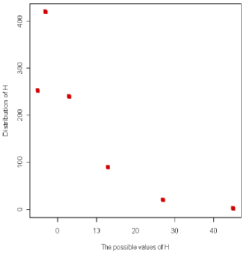
Figure 1: Exact distitribution of the energy function when there are 10 traders.

In the Table 1 are the exact numerical values of the energy distribution.

$h$	$-5$	$-3$	3	13	27	45
Number of occurrances	252	420	240	90	20	2
Probability	0.246	0.41	0.234	0.088	0.0195	0.00195

Table 1: The exact distribution values of the energy function when there are 10 traders.

3.4 Hypothesis test of independence

If there is only weak interaction between the traders, then the Hamiltonian is more likely to attain smaller values. If the interactions are stronger, then larger values of the Hamiltonian is more likely and one talks about magnetization, which could be an indicator of, or even a cause of, bubbles and crashes on the market. Therefore methods to state wheter the values of the observed Hamiltonian is in some dangerous region is of vital importance to decision makers and inderictly to the whole society.

In order to see if the value of the Hamiltonian deviates from zero to such an extent that dangerous development is indicated, the correct distribution is needed. If the Hamiltonian approaches the critical value, the system may be in a dangerously instable state and a bubble or a crash on the market can appear.

Assume that we make $n$ observations $x_{1},x_{2},\ldots,x_{n}$ of the system. Then the corresponding Hamiltonian values $h_{1},h_{2},\ldots,h_{n}$ are calculated and categorized into $K$ classes. If the number of traders are 10 (as in the previous example), then the we may have 6 classes corresponding to the 6 possible states of the Hamiltonian. But of course we may define these classes in any way we choose.

Strong interactions as opposed to near independence is reflected by the hypotheses

$$\left\{\begin{array}[]{l}H_{0}:\beta=0\\ H_{1}:\beta>0\end{array}\right.$$

To have argument for dependence, i.e. to prove $H_{1}$, the statistic

$$S\;=\;\sum_{k=1}^{K}\frac{(O_{k}-E_{k})^{2}}{E_{k}}$$

may be used, where $O_{k}$ is the number of observations in klass $k$, and $E_{k}$ is the expected number of observations in class $k$ according to the distribution of $S$ under $H_{0}$ which is $\chi^{2}_{k-1}$. Thus the null hypothesis is rejected at level $\alpha$ of significance for values of $S$ greater than $C$ which is $1-\alpha$ percentile of the $\chi^{2}$ distribution with $k-1$ degrees of freedom.

Example 2

Let us consider the data from the Swedish steel market for the October 22, 2008. We have the traders and buyers with certain moments of trading. To analyze these data we will collect information about trading by dividing the time on parts of each about 10 minutes. We than have the ten most active traders (AVA, CSB, DBL, ENS, EVL, MSI, NDS, NON, SHB, SWB) and twenty intervals of activity. Let us consider the Hamiltonian for these traders. The result is in Table 2.

State	$-5$	$-3$	$3$	$[13,45]$
Number of occurances	2	13	4	1
Expected number of occurance	4.92	8.2	4.688	2.19

Table 2: The frequencies of observations divided into four classes.

Thus $N=10$ and $K=4$. The value of the test statistic in this case is

$${\textstyle\frac{(2-4.92)^{2}}{4.92}+\frac{(13-8.2)^{2}}{8,2}+\frac{(4-4.688)^{2}}{4.688}+\frac{(1-2.19)^{2}}{2.19}}\;=\;5.29\;<\;7,8147\;=\;\chi^{2}_{3}(0.05)$$

This means that we can not reject the hypothesis of independence on level 5% of significance (or any lower level). As a matter of fact the $p$-value of $S$ in this case is $0.15175$ so dependence can not be proved on any reasonable level of significance.

4 Discussion

In this thesis we investigated a new space-time model for interacting agents in the financial market. First we reviewed the history of the Ising model and some other Ising-type models. Then the Ising model, Curie-Weiss model and some modifications of these models were formally presented. Also we considered one way of finding the critical temperature of the market. A new space-time model was developed and necessary and sufficient conditions for its stationarity were found. The non-linear sensitivity of market global properties in terms of temperature parameter changes was investigated. The critical temperature for this model was analytically derived.

The distribution of the Hamiltonian was analyzed using its dependence with the magnetization of the market and the exact distribution was calculated. The conditional expectation and variance of the Hamiltonian were found and the stationary distribution was obtained. Then the exact distribution of the Hamiltonian for 10 traders was calculated, and the expected distribution was confirmed. Hypothesis test for independence between agents was considered for the Swedish steel market and it showed that there is no evident critical situation on the market at the time of this dataset.

The parameter reflects how strongly traders are influenced by each other in the market. It can signalize risk for a crash or a bubble in the market. Therefore it is very important that its analysis is accurate in such situations. What remains for future work? We could try a lot of real data and compare inferential results relying on this model to observable quantities generally accepted as a measure of health of the situation on the market. Also we can consider a bigger ammount of traders to have a more exact $p$-value in the hypothesis testing. Then we can estimate the amount of interaction for our model using e.g. maximum likelihood estimator. Here exists also the possibility to develop hypothesis testing based on a time dependent model. Also interesting to find out how good this model is to explain volatility clustering.

References

- [1] Domb, C., Green, M.S. and Lebowitz, J.L. (2001) Phase Transitions and Critical Phenomena. Academic Press.
- [2] Föllmer, H. (1974) Random Economies with Many Interacting Agents. Journal of Mathematical Economics, 1(1), 51–62.
- [3] Hartmann, A.K. and Weigt, M. (2005) Phase Transistions in Combinatorial Optimization Problems. Wiley-VHC.
- [4] Järpe, E. (2005) An Ising-Type Model for Spatio-Temporal interactions. Markov Processes and Related Fields, 11, 535–552.
- [5] Kaizoji, T. (2000) Speculative Bubbles and Crashes in Stock Market: An Interacting-Agent Model of Speculative Activity. arXiv.org.