The Mass-Size Relation from Clouds to Cores. I. A new Probe of Structure in Molecular Clouds

Abstract

We use a new contour-based map analysis technique to measure the mass and size of molecular cloud fragments continuously over a wide range of spatial scales ($0.05\leq r/{\rm pc}\leq 10$), i.e., from the scale of dense cores to those of entire clouds. The present paper presents the method via a detailed exploration of the Perseus Molecular Cloud. Dust extinction and emission data are combined to yield reliable scale-dependent measurements of mass.

This scale-independent analysis approach is useful for several reasons. First, it provides a more comprehensive characterization of a map (i.e., not biased towards a particular spatial scale). Such a lack of bias is extremely useful for the joint analysis of many data sets taken with different spatial resolution. This includes comparisons between different cloud complexes. Second, the multi-scale mass-size data constitutes a unique resource to derive slopes of mass-size laws (via power-law fits). Such slopes provide singular constraints on large-scale density gradients in clouds.

1. Introduction

Some of the most fundamental properties of molecular clouds are the mass and size of these clouds and their substructure. Today, these properties are well constrained: we know the masses and sizes of dense cores in molecular clouds ($\lesssim 0.1~{}\rm pc$ size; e.g. Motte et al. 1998, Johnstone et al. 2000, Hatchell et al. 2005, Enoch et al. 2007), and those of clumps (some $0.1~{}\rm pc$) and clouds ($\gtrsim 10~{}\rm pc$) containing the cores (e.g., Williams et al. 1994, Cambrésy 1999, Kirk et al. 2006; see Williams et al. 2000 for definitions of cores, clumps, and clouds). We do, however, not know much about the relation between the masses and sizes of cores, clumps, and clouds: traditionally, every domain is characterized and analyzed separately. As a result, it is still not known how the core densities (and thus star-formation properties) relate to the state of the surrounding cloud.

In principle, the relation between the mass in cloud structure at large and small spatial scales is described by mass-size relations. Larson (1981) presented one of the first studies of such relations. He concluded (in his Eq. 5) that the mass contained within the radius $r$ obeys a power-law,

$$m(r)=460\,M_{\sun}\,(r/{\rm pc})^{1.9}\,.$$ (1)

Most subsequent work refers to this relation as “Larson’s 3^rd law”, and replaces the original result with $m(r)\propto r^{2}$ (e.g., McKee & Ostriker 2007). This “law of constant column density” (with respect to scale, $r$) is now considered one of the fundamental properties of molecular cloud structure (e.g., reviews by Ballesteros-Paredes et al. 2007, McKee & Ostriker 2007, Bergin & Tafalla 2007). This relation has, however, never been re-examined comprehensively on the basis of up-to-date data. It is, e.g., not clear whether recent dust extinction and emission work is consistent with $m(r)\propto r^{2}$.

Further, the limitations of available structure identification schemes (such as CLUMPFIND; Williams et al. 1994) forced past studies to break cloud structure maps up into discrete fragments. These fragments typically have a size slightly larger than the map resolution. As a consequence, the cloud structure is only probed in a narrow spatial domain; the largest spatial features in a given map are, for example, usually not characterized. Today, approaches permitting automatic examination of a continuous range of spatial scales are available. Rosolowsky et al. (2008b), in particular, provide software for such studies (their dendrogram analysis); our work would be impossible without the work by Rosolowsky et al.. Such software permits derivation of spatially more comprehensive mass-size relations than possible in the past.

In this series of papers, we combine contemporary column density observations of high sensitivity with a new data analysis technique to examine the mass-size relation in molecular clouds for a continuous range of spatial scales of order $0.01~{}{\rm to}~{}10~{}\rm pc$. We rely on extinction maps of molecular clouds (here: Ridge et al. 2006), as well as maps of dust emission (Enoch et al., 2006). Following the terminology of Peretto & Fuller (2009), we define “cloud fragments” in the maps as regions enclosed by a continuous column density contour, and derive their mass and size at various contour levels. This is implemented using algorithms introduced by Rosolowsky et al. (2008b).

The first two papers in this series establish our analysis approach (part I, the present paper) and explore several clouds in the solar neighborhood ($\lesssim 500~{}\rm pc$; part II). Section 2 of the present paper describes our cloud fragment extraction and characterization scheme. In Sec. 3 we provide a first idea how basic physical properties and observational limitations affect the mass-size measurements. This includes a comparison to results obtained using the CLUMPFIND algorithm. A detailed discussion of analysis uncertainties is presented in Sec. 4. These are explored using data for the Perseus Molecular Cloud. We also explain how dust emission and extinction data can be combined for a given cloud.

Section 5.1 briefly describes how the new map analysis scheme might help to advance star formation research. As we describe there, it will help to jointly analyse data taken at different spatial resolution. This is a key feature in the age of multi-wavelength and multi-resolution studies. We conclude with a summary in Sec. 5.2.

a) input map	b) mass-size data

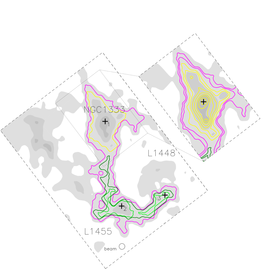
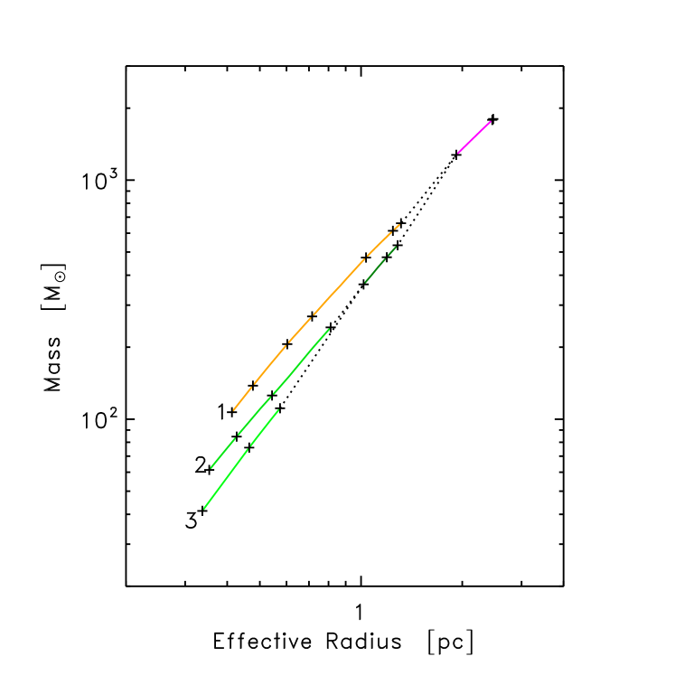
Figure 1.— Fundamental concept of mass-size measurements. Panel (a) shows an example column density map for the Perseus molecular cloud, where labels refer to individual star-forming regions. Such maps usually contain several local maxima (numbered crosses in map). We pick one of these maxima, and draw contours at constant column density around this peak (map inset). For each contour, we measure mass and size. These measurements can then be placed in a mass-size plot, as marked by crosses in panel (b). When a map contains several maxima, it can be divided into cloud fragments where contours just contain a single maximum (light green and yellow boundaries in panel [a]), two of these (dark green boundary), or even more (magenta contour). In this sense, mass-size measurements for contours contained in one of these areas are related. These relations are highlighted by colored lines in panel (b); the color refers to the map region from where the measurements are taken, and numbers indicate the central column density peak of each fragment. When two fragments blend into a combined one that contains both, mass and size measurements jump discontinuously from those of the individual fragments to those for the combined one. These jumps are indicated by dotted lines.

2. Method

2.1. Processing of Contour Maps

Consider some column density map containing a number of local maxima, as sketched in Fig. 1 (a). In this map, cloud fragments can be identified as structures bound by some continuous contour. To characterize these, we pick one of the column density maxima, and measure the mass, $m$, and area, $A$, contained within each column density contour containing this peak. Here, we use the effective radius,

$$r=(A/\pi)^{1/2}\,,$$ (2)

to quantify $A$. By following the trends from contour to contour, as shown in Fig. 1 (b), one can construct a mass-size relation for every cloud fragment. Strictly speaking, we do thus construct mass-area diagrams. In practice, however, $r$ is arguably a more intuitive variable than $A$.

Some contours may contain several local maxima. They represent composite fragments. To give an example based on Fig. 1, the region bound by the dark-green contour consists of the two regions marked in lighter shades of green, and the magenta contour contains the fragments marked in yellow and dark-green. Merging of two fragments occurs at the first column density contour containing both of the fragments. In our analysis, we enforce that only two fragments can merge at a time.

During a merger, mass and size jump discontinuously from the pre-merger situation, $m_{i}$ and $r_{i}$, to their post-merger value, $m=m_{\rm A}+m_{\rm B}$ and $r=(r_{\rm A}^{2}+r_{\rm B}^{2})^{1/2}$. This yields gaps in the mass-size relation (Fig. 1 [b]). The merger information is preserved during processing, so that it is possible to look up which fragments are contained within others.

Our map characterization scheme is thus closely related to the one employed by Peretto & Fuller (2009). Like us, these authors measure sizes and masses for regions bound by lines of constant column density. The schemes differ in the number of contours considered: we use a very large number ($10^{2}$ to $10^{3}$), where Peretto & Fuller only consider two contours per cloud.

In practice, we use the dendrogram (i.e., tree analysis) code presented by Rosolowsky et al. (2008b) for automatic processing of the maps. A minimum significant contour has to be set for every region; emission below this limit is not characterized here. It is further necessary to specify a minimum contrast between peaks, in order to identify significant central maxima for the objects. These threshold column densities and contrasts are listed separately for every region in the following. The identified maxima are required to be spaced by more than one spatial resolution element. Again, this parameter is noted separately for every map. In this work, all sources with an effective diameter (i.e., $2r$) smaller than twice the map resolution are rejected and are treated as parts of enveloping objects.

In the terminology of Rosolowsky et al., our mass measurement approach (i.e., integrate column density within some contour) corresponds to their “bijection paradigm”. Such mass measurements, e.g. made towards a dense core, always give a sum over several spatially overlapping components (e.g., some fraction of the dense core, plus some fraction of its envelope). This is not a problem, if properly taken into account in the later analysis. Other choices are possible (e.g., the “clipping paradigm” of Rosolowsky et al.), but they are less intuitive and even harder to model. Also, most previously existing data has been published effectively adopting the bijection paradigm.

2.2. Mass Estimates

As a first example, below we present a mass-size analysis of Perseus, based on column densities derived from 2MASS-derived extinction data. As explained by Ridge et al. (2006), the map is derived in terms of magnitudes of visual extinction, $A_{V}$. We convert this to $\rm H_{2}$ column densities using the relation

$$N_{\rm H_{2}}=9.4\times 10^{20}~{}{\rm cm^{-2}}\,(A_{V}/{\rm mag})$$ (3)

(Bohlin et al., 1978). Mass surface densities, $\Sigma$, can then be derived as

$$\Sigma=\mu_{\rm H_{2}}\,m_{\rm H}\,N_{\rm H_{2}}\,,$$ (4)

where $\mu_{\rm H_{2}}=2.8$ is the mean molecular weight per $\rm H_{2}$ molecule (Kauffmann et al., 2008) and $m_{\rm H}$ is the weight of the hydrogen molecule. In practice, $\Sigma=0.047~{}{\rm g\,cm^{-2}}\,(N_{\rm H_{2}}/10^{22}~{}{\rm cm^{-2}})=226~{}M_{\sun}\,{\rm pc^{-2}}\,(N_{\rm H_{2}}/10^{22}~{}{\rm cm^{-2}})$, or $A_{V}=227.5~{}{\rm mag}\,(\Sigma/{\rm g\,cm^{-2}})$. The mass is then derived by integrating the mass surface density, $m=\int\Sigma\,{\rm d}A$. For this we adopt a Perseus distance of $260~{}\rm pc$ (Cernis, 1993).

Goodman et al. (2009b) present a comparison of column density tracers for the Perseus region. After studying column density maps based on dust extinction (from 2MASS data), dust emission (from IRAS imaging), and line emission data (from large field $\rm{}^{13}CO$ [1–0] mapping), they conclude that extinction-based maps provide the best available information on a cloud’s spatial mass distribution. Extinction-based column densities deviate by $\sim 25\%$ from those derived from other tracers (after removing global offsets between estimates, e.g. due to the choice of dust opacities). The true column density is supposedly in between these estimates. If every tracer has a similar scatter with respect to the true column density, this scatter would then be $\sim 25\%/2^{1/2}\approx 18\%$ for all tracers. Extinction-based estimates of the column density do probably deviate by a lower amount from the true value. Here, we thus adopt a systematic uncertainty of $\lesssim 15\%$ for extinction-based mass estimates in Perseus.

Young stars embedded in the clouds can further bias extinction observations, given their red intrinsic colors. This bias is particularly significant towards clusters, such as NGC1333 and IC348 in Perseus. We do not exclude these regions from our study, but measurements towards the clusters should be interpreted with particular caution.

2.3. Example Map

Figure 2 shows the aforementioned extinction map for Perseus. The two most prominent star-forming regions in Perseus, NGC1333 and IC348, manifest as extended extinction structures in this map. Fragments of very small size (e.g., $\lesssim 0.1~{}\rm pc$), like dense cores around individual young stellar objects, are not visible in the map, due to its too poor spatial resolution ($5\arcmin$, corresponding to $\approx 0.4~{}\rm pc$). Section 4.2 shows how such structures can still be bootstrapped into mass-size studies.

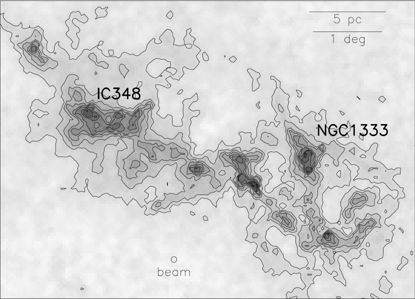
Figure 2.— Example column density map for Perseus, presented in terms of visual extinction, $A_{V}$. The map is taken from Ridge et al. (2006). Contours are drawn in steps of $1~{}\rm mag$, starting at $2~{}\rm mag$. Labels indicate the rough position of the star forming regions NGC1333 and IC348.

Figure 3 presents the mass-size data derived from the Perseus extinction map. This diagram reveals that the Perseus complex has a total (effective) radius of $8~{}\rm pc$ and a total mass of $1\times 10^{4}~{}\rm M_{\odot}$. The properties from contours containing the two major stellar clusters, NGC1333 and IC348, are highlighted by bold black lines. As one may naively expect, the cloud fragments enclosing these clusters are, at given radius, the most massive fragments within the cloud complex. This analysis also reveals fragments that are, again at given radius, much less massive than the regions containing the clusters. As discussed in the next paragraphs, the column density sensitivity of the map sets a radius-dependent lower limit to the masses that can be detected in a given map. Fragments of a mass much lower than those shown here may thus well exist in Perseus. Eventually, at sufficiently large radius, most of the contour-bound objects found merge into a single fragment containing essentially all of the Perseus molecular cloud.

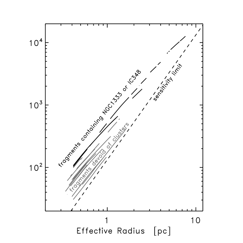
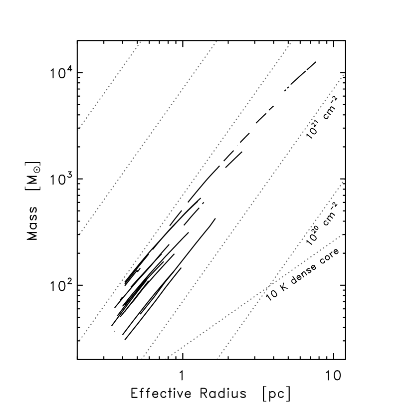
Figure 3.— Mass-size relation for the Perseus molecular cloud. Compared to Fig. 1, we only keep the lines connecting related measurements. The top panel describes the data in detail. Bold solid lines indicate data for fragments either containing NGC1333 or IC348. Light solid lines show observations for regions not associated with these clusters. The dashed line gives the sensitivity limit of the analysis. In the bottom panel we present the data in the context of reference mass-size relations. Dotted lines indicate mean $\rm H_{2}$ column densities, $\langle N_{\rm H_{2}}\rangle$, respectively the mass-size relation for a singular hydrostatic equilibrium sphere supported by isothermal pressure from gas at $10~{}\rm K$ temperature (see Sec. 3.1 for both).

In the processing of the map, we have used a minimum threshold extinction of $2~{}\rm mag$. This limit is much larger than the noise level of $0.4~{}\rm mag$ (Ridge et al., 2006) and rejects the signal from background extinction structures not related to the cloud. Correspondingly, we cannot detect fragments with a mean extinction below $2~{}\rm mag$. Given the relation between mass, size and mean column density (Eq. 5), this minimum column density sets a lower limit to the detectable mass. Substitution of the minimum column density, $N_{\rm H_{2},min}$ (in Eq. 5; note that $\langle N_{\rm H_{2}}\rangle\geq N_{\rm H_{2},min}$), gives sensitivity limits like the one shown in Fig. 3. The minimum contrast between peaks is required to be the noise level times a factor 3, i.e. $1.2~{}\rm mag$. The spatial resolution of the map is $5\arcmin$; we do therefore require the maxima to be separated by at least 3 pixels ($7\farcm 5$), and objects with a radius smaller than $5\arcmin$ are rejected as being unphysical.

3. Properties of Mass-Size Data

Some mathematical and physical laws governing the properties of mass-size data have to be heeded, if a meaningful interpretation of the observations is desired. Here we list the most fundamental of these.

3.1. Reference Relations

A number of reference mass-size relations can help to navigate within the observational data more intuitively. They are in part derived assuming a spherical geometry for cloud fragments. The assumption of spherical symmetry may not be appropriate, though. This caveat should be kept in mind when using the following reference relations.

Mass and size measurements can be used to calculate the mean mass surface (or column) density of a fragment, $\langle\Sigma\rangle=m(r)/A(r)$. Conversely, one can draw lines of constant mass surface density, $m(r)=\langle\Sigma\rangle\,\pi\,r^{2}$. Conversion to column density, and substitution of the aforementioned constants, yields

$$m(r)=71\,M_{\sun}\,(\langle N_{\rm H_{2}}\rangle/[10^{21}~{}{\rm cm^{-2}}])\,(r/{\rm pc})^{2}\,.$$ (5)

These lines are drawn in most mass-size plots presented here (e.g., Fig. 3). Equation (5) implies one of the most important properties of mass-size data: since column density decreases with increasing radius, the observed mass-size relations must be flatter than $m(r)\propto r^{2}$.

Equation (5) can actually be used to transform our results into the analytical diagram presented by Tan (2007; column-density vs. mass). Our study goes beyond the work by Tan (2007) in that it systematically populates the parameter space with observational data.

For spherical clouds, the mean density is $\langle\varrho\rangle=m(r)/(4/3\,\pi\,r^{3})$. The corresponding mass-size relation reads $m(r)=4/3\,\pi\,\langle\varrho\rangle\,r^{3}$, or

$$m(r)=282\,M_{\sun}\,(\langle n_{\rm H_{2}}\rangle/[100~{}{\rm cm^{-3}}])\,(r/{\rm pc})^{3}\,,$$ (6)

where we substitute the density of $\rm H_{2}$ molecules, $n_{\rm H_{2}}=\varrho/(\mu_{\rm H_{2}}\,m_{\rm H})$.

In part II of this series, we shall study spherical power-law density profiles, $\varrho(s)\propto s^{-k}$ (where $s$ is the radius), as models for the observed mass-size relations. We show that

$$\varrho(s)\propto s^{-k}\quad\Leftrightarrow\quad m(r)\propto r^{3-k}\,.$$ (7)

The slope of the mass-size relation is therefore related to the slope of the density law. A density profile $\varrho(s)\propto s^{-2}$ is often adopted to describe dense cores (see Dapp & Basu 2009 for a discussion). This gives a mass-size relation $m(r)\propto r$. In hydrostatic spheres supported by isothermal pressure, mass, size, and gas temperature are related by

$$m(r)=2.6\,M_{\sun}\,\left(\frac{T_{\rm g}}{10~{}\rm K}\right)\,\left(\frac{r}{0.1~{}\rm pc}\right)$$ (8)

(see Kauffmann et al. 2008, Eq. 13). For gas temperatures $T_{\rm g}=10~{}\rm K$, one obtains the model relation drawn in most mass-size diagrams of this paper (e.g., Fig. 3).

We stress that we obtain two-dimensional mass-size relations from column density maps. These are related to, but not identical with, mass-size laws obtained from three-dimensional density maps. This is illustrated by the experiments conducted by Shetty et al. (2010, submitted) who use the fragment identification technique also used by us. Their analysis is based on three-dimensional numerical simulations of turbulent clouds. As part of their experiments, they fit power-laws (similar to Eq. 1) to their mass-size data. For their particular set of simulations, the exponent derived in this fashion is similar to the number of dimensions used for mass measurements (i.e., 3 when based on density, and 2 when based on column density). This underlines that the number of dimensions considered has to be kept in mind. Note, though, that these details do not compromise mass-size measurements as a tool for cloud structure analysis. Observed mass-size laws unambiguously summarize actual cloud structure. Only their interpretation is sensitive to the assumed geometry.

3.2. Relation to CLUMPFIND-like Results

The approach chosen here constitutes one of several possible choices to measure the mass and size of objects in maps. Another popular approach is to use the CLUMPFIND algorithm (Williams et al., 1994). This method uses contours to break emission up into several objects, just as done here. CLUMPFIND-extracted boundaries do, however, not necessarily follow contours. This is a major difference to our method, where objects are always bound by some column density contour. Based on this fact alone, CLUMPFIND and our approach will thus extract very different objects. Goodman et al. (2009a) illustrate this problem comprehensively.

Further, CLUMPFIND does not allow for hierarchical structure, i.e., fragments containing other fragments. For example, CLUMPFIND will never determine the integral properties of the entire cloud, since the cloud is usually broken up into many independent fragments. The relation of CLUMPFIND-results to cloud hierarchy is studied by Pineda et al. (2009).

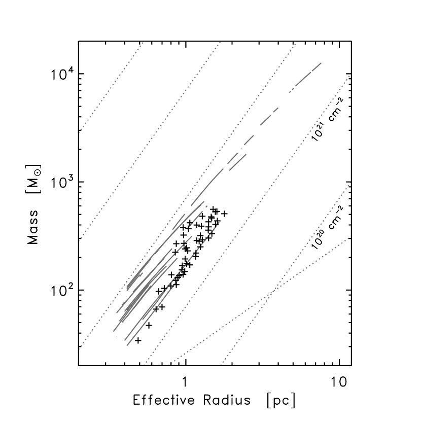
Figure 4.— CLUMPFIND (crosses) and dendrogram mass-size results (lines) for the extinction map presented in Fig. 2. The two approaches yield broadly similar, but not directly related results.

Figure 4 compares mass and size measurements from CLUMPFIND to those from our approach. Both characterizations are based on our Perseus extinction map. To initiate CLUMPFIND, we choose contours as close as possible to the parameters used in our contour-based segmentation (Sec. 2.3); the contour spacing is $1.2~{}\rm mag$, with the lowest contour at $2~{}\rm mag$. Still, this CLUMPFIND segmentation yields objects that are only remotely related to the regions extracted by our method. To start with, CLUMPFIND extracts 52 peaks enclosed by individual clumps, where our method only identifies 17 significant peaks. This discrepancy is a consequence of CLUMPFIND’s relaxed peak identification criterion: every local peak encircled by a continuous contour is considered significant, independent of the depth of the column density dip towards the next peak. There is thus no well-defined correspondence between regions identified by the different algorithms.

To characterize the relation between objects extracted by different methods in some sense, we inspect the structure around the 17 significant column density peaks found by our method. For every such peak, we identify the CLUMPFIND object containing this peak. The mass of the latter clump can then be compared to our results, taken at the clump’s radius. Because of merging of objects, our method does not provide a mass measurement for every possible radius (consider, e.g., the evolution of mass-size measurements starting from peak 3 in Fig. 1[b]). For those cases where mass measurements exist for the CLUMPFIND-derived radius, we find that CLUMPFIND gives masses of order 55% to 95% of the masses derived by our approach.

In summary, mass and size measurements from CLUMPFIND are thus broadly compatible with our results. By this we mean that the CLUMPFIND-derived mass-size measurements reside in the space spanned by our own measurements. There is, however, no good correspondence on a detailed level.

4. Perseus in Detail

Given the tools derived above, it is now possible to characterize the mass-size relation for Perseus. While doing so, we also evaluate uncertainties affecting our analysis. In a final step, we extend the analysis to clouds other than Perseus.

4.1. Mass Uncertainty

To explore the impact of noise on mass measurements, we run Monte-Carlo experiments in which we add artificial Gaussian noise of root-mean-square (RMS) amplitude $\sigma(m_{i})$ to the map before structure characterization (where $m_{i}$ is the mass per pixel). Such trials are presented in Fig. 5(a). Comparison of the derived mass-size data to the one from the original map does then reveal the impact of noise. In our experiments, we find that

$$\frac{\sigma(m)}{m}=6\,\frac{\sigma(m_{i})}{m}\,\frac{r}{r_{\rm beam}}$$ (9)

is an upper limit to the noise-induced mass changes, $\sigma(m)$. In this, $r_{\rm beam}$ is the beam radius and the numerical constant does slightly depend on the number of pixels per beam.

Equation (9) follows from Gaussian error propagation of $m=\Sigma_{i}m_{i}$. The numerical constant is increased by a factor 3, though, to provide a strict upper limit to uncertainties. To test for non-Gaussian sources of error, we validate Eq. (9) by comparing the original data with those derived from maps with additional noise. For any given structural branch with $r<2~{}\rm pc$, Eq. (9) is indeed found to set an upper limit to the mass deviation at given radius, following the noise experiments depicted in Fig. 5(a). For larger radii, a small (but significant) additional uncertainty of $\sim 1\%$ has to be included to capture non-Gaussian sources of error.

In our study, the relative uncertainty of column density estimates (i.e., $\sigma(m_{i})/m_{i}$) is $\leq 1/5$ in characterized regions (given extinction noise levels and selection thresholds of $0.4~{}\rm mag$ and $2.0~{}\rm mag$, respectively). Further, the mass is at least as large as the one at the sensitivity limit (Fig. 3[a]), $m>\pi\,m_{i,\rm min}\,(r/r_{\rm beam})^{2}$ (in our map, the beam contains, by area, $\pi$ pixels). Substitution of these parameters in Eq. (9) give uncertainties of 19% for the smallest extracted features (for which $r=2r_{\rm beam}$) located just at the sensitivity limit. Since $\sigma(m)/m\propto\langle N_{\rm H_{2}}\rangle^{-1}\,r^{-1}$ (via substitution of Eq. [5]), larger regions well above the detection threshold will suffer lesser uncertainties, $\ll 10\%$.

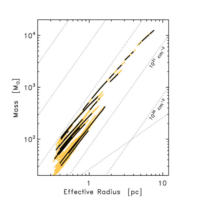
	(a) impact of noise
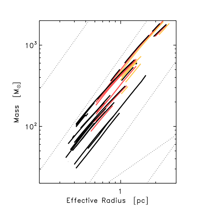
	(b) impact of smoothing

Figure 5.— Impact of noise (top) and limited spatial resolution (bottom) on mass-size measurements. Note that the size and mass scale differ between the panels. Noise and resolution are explored using artificial maps created by adding noise to (top), respectively smoothing of (bottom), the observed data for Perseus (Sec. 4.1). Differences between the input data and the properties of the artificial maps are due to these biases. The original input data is drawn in black. yellow lines in the top panel show mass-size relations from maps with additional noise similar to the observed one ($0.4~{}\rm mag$). Red and yellow lines in the bottom panel present mass-size relations for maps with a resolution worsened to $r_{\rm beam,f}/r_{\rm beam,i}=3/2$ and $5/2$, respectively (and features with $r<2\,r_{\rm beam,f}$ removed). At given radius, both biases just induce moderate changes in mass (Sec. 4.1).

In later papers, we will compare the properties of clouds that are located at different distances. Since the angular resolution of the observations is about constant, an increase in distance implies a decrease in physical resolution. To first order, this decrease in physical resolution corresponds to smoothing of the map. We explore the impact of smoothing by extracting mass-size data from smoothed maps of the Perseus cloud, as demonstrated in Fig. 5(b).

Smoothing does effectively mean that mass is transferred to larger scales. For fixed radius, smoothing does thus imply a reduction in mass. To estimate this reduction, consider a region of effective radius $r$. After smoothing, the mass contained in this region will be smeared our over an area of radius $r^{\prime}\sim r_{\rm ini}+r_{\rm k}$. In this, $r_{\rm k}=(r_{\rm beam,f}^{2}-r_{\rm beam,i}^{2})^{1/2}/(\ln(2))^{1/2}$ is the effective radius of the smoothing kernel required to go from the initial to the final beam radius of the map during smoothing, $r_{\rm beam,i}\to r_{\rm beam,f}$. Very approximately, after smoothing the mass retained in the initial area will be of order of the fraction of the initial area to the one after smoothing, $r^{2}/(r+r_{\rm k})^{2}$.

After rearrangement (and using $r_{\rm k}\ll r$), we find that the smoothing-induced mass bias should obey a relation of the form

$$\frac{\Delta m}{m}\approx 0.2~{}{\rm to}~{}0.3\cdot\left[1-\frac{1}{(1+r_{\rm k}/r)^{2}}\right]\,.$$ (10)

To allow for more realistic source geometries, the numerical constant must be derived from experiments with actual data. We use the smoothing experiments shown in Fig. 5(b) for this purpose. With these parameters, Eq. (10) describes the relative mass bias for all structure branches in our example map.

In our study, we only consider regions with radii larger than twice the effective beam radius, $r>r_{\rm beam}$. Substitution of this (with $r_{\rm beam,i}=0$, since the true distribution on the sky has infinite resolution) in Eq. (10) shows that the mass of regions with a radius similar to the beam diameter may be underestimated by not more that 20%, and by less for larger fragments.

4.2. Combining Dust Emission and Extinction Data

Our Perseus extinction map has a spatial resolution of $5\arcmin$ ($0.4~{}\rm pc$). It cannot be used to characterize much smaller fragments, such as dense cores of $\lesssim 0.1~{}\rm pc$ size. This limitation can, however, be overcome when including mass-size data from additional data sets.

4.2.1 Basic Concept

For Perseus, Enoch et al. (2006) present a Bolocam map of dust emission in Perseus at $1.1~{}\rm mm$ wave length. The beam width at half sensitivity is $31\arcsec$, corresponding to $0.04~{}\rm pc$. At these wave lengths, the continuum emission of dust at temperature $T_{\rm d}$ is optically thin, and so the observed dust continuum emission intensity, $I_{\nu}$, is a direct measure of the column density along a given line of sight,

$$I_{\nu}=\mu_{\rm H_{2}}\,m_{\rm H}\,\kappa_{\nu}\,N_{\rm H_{2}}\,B_{\nu}(T_{\rm d})$$ (11)

(see Kauffmann et al. 2008 for full details), where $B_{\nu}$ is the Planck function, and the dust opacity, $\kappa_{\nu}$, is evaluated per total gas mass. Column density maps from dust emission can then be contoured and analyzed as described before (Sec. 2) to derive mass-size data for the fragments in the dust emission map.

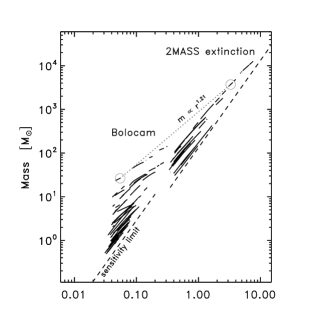
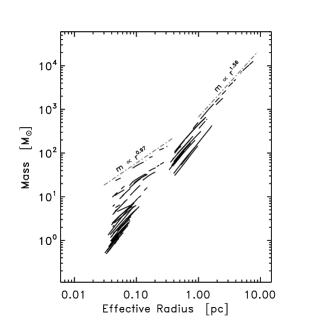
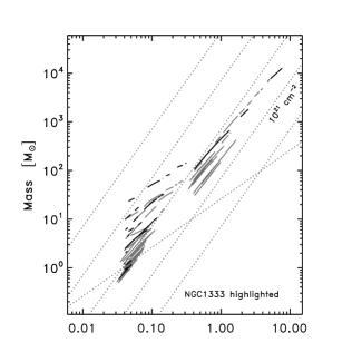
Figure 6.— Mass-size data for Perseus (solid lines). The data are from dust extinction maps probing large spatial scales, and Bolocam dust emission observations sensitive to small ones. The left panel highlights the nature of the data; dashed lines give the instrument-dependent sensitivity limits. Circles and the dotted line indicate calculation of the global mass-size slope (Sec. 4.3). The middle panel highlights slopes derived by matching power-laws to parts of the data. Tangential slopes (Sec. 4.4) are derived in the same fashion, but for infinitesimal radius ranges. The right panel presents Perseus in the context of the reference mass-size relations from Sec. 3.1. Here, black solid lines highlight Bolocam-detected fragments in NGC1333, as well as the extinction-probed fragments containing this cluster. Other data are drawn using grey solid lines.

Figure 6 combines the Bolocam-derived mass-size measurements with the extinction-based ones. Spatially, they are separated by a gap, since Bolocam ($\lesssim 2\arcmin$) and 2MASS extinction maps ($\gtrsim 5\arcmin$) probe different spatial scales. The extinction-identified fragments do, however, contain the Bolocam-derived ones. For example, shading in Fig. 6 highlights Bolocam-detected fragments contained in the extinction peak harboring NGC1333.

4.2.2 Relative Calibration of Dust Opacities

Bianchi et al. (2003) studied B68 to examine the relation of mass estimates from dust extinction and emission. They find relative differences by factors of $1~{}{\rm to}~{}\sim 2.35$, when adopting opacities for Ossenkopf & Henning (1994) dust grains with thin ice mantles that coagulate for $10^{5}~{}\rm yr$ at $10^{6}~{}\rm cm^{-3}$ density (see Kauffmann et al. 2008, Table A.1, for numerical values). This is consistent with previous studies of this subject, including sources as diverse as diffuse clouds and galaxies (see references in Bianchi et al. 2003). If one fixes the opacity used for extinction observations, it thus appears that the the Ossenkopf & Henning (1994) model opacities near $1~{}\rm mm$ wave length are too large by an average factor $1.5\approx 2.35^{1/2}$.

In our emission-based column density estimates, we do therefore basically adopt the aforementioned Ossenkopf & Henning (1994) opacities for dust emission observations near $1~{}\rm mm$ wave length, but scale these down by a further factor 1.5 to bring mass estimates from extinction into harmony with those from dust emission. As seen in Fig. 6, this procedure yields reasonable results, since the dust emission and extinction observations for NGC1333 match within less than a factor 2 (i.e., when comparing the masses of the most massive Bolocam-detected fragment to the one of the least massive 2MASS-identified fragment). Incorrect assumptions about dust temperatures may cause most of this offset (see below).

To some extent, correction factors between masses from dust emission and extinction are also influenced by spatial filtering affecting bolometer observations (Sec. 4.2.4). Future studies need to address this problem in more detail. Still, the aforementioned scaling factor aligns dust emission and extinction studies, which is the only aspect needed in our present study.

4.2.3 Dust Temperatures

For Perseus, Rosolowsky et al. (2008a) estimate gas temperatures between $9~{}\rm K$ and $18~{}\rm K$. Assuming that dust and gas temperatures are similar, we do therefore adopt a temperature of $(12.5\pm 2.5)~{}\rm K$ in our mass estimates. This temperature uncertainty results in a relative mass uncertainty of $\sim 20\%$ for Perseus. A few sources may have dust temperatures, and mass biases, outside of this range.

4.2.4 Impact of Spatial Filtering

Like all other upcoming, present, and past ground-based bolometer-derived dust emission maps (Kauffmann et al., 2008), the Bolocam maps of Perseus are not sensitive to structure larger than some instrument-dependent spatial scale. In its impact, this problem is similar to the spatial filtering in interferometric imaging. For Bolocam, Enoch et al. (2006) show the filtering scale to be of order $1\arcmin$ to $2\arcmin$ radius.

Quantitatively, this removal of large-scale structure has an influence opposite to the impact of smoothing (Sec. 4.1): here, the relative mass-loss increases with spatial scale. This bias has to be considered carefully when using emission-based mass-size measurements for analysis. Obviously, the true mass will be larger than the observed value. Filtering in bolometer maps is unfortunately too complex to be characterized in a compact fashion; see Kauffmann et al. (2008) for a few rules of thumb. For the particular case of the Bolocam maps of Perseus, Enoch et al. (2006) report losses $\leq 10\%$ for radii $\leq 1\arcmin$, but do not sufficiently explore larger objects.

4.3. Global Trends in Maximum Mass for given Size

The mass-size tendencies seen, e.g., in Fig. 6 suggest to describe these trends with power laws of the form

$$m(r)=m_{0}\,(r/r_{0})^{b}\,.$$ (12)

In this, $b$ is the slope of the relation, and $m_{0}$ is the intercept. As shown in Fig. 6, such laws trace, e.g., the mass-size relation of the most massive fragments in the $0.04\leq r/{\rm pc}\leq 0.3$ and $1\leq r/{\rm pc}\leq 8$ radius intervals with maximum deviations of $\pm 6\%$.

Beyond such detailed descriptions of individual features, power-laws can be used to capture more global aspects of a cloud’s structure. Consider, for example, the relation between the maximum fragment masses, $m_{\rm max}$, observed at radii of $r_{\rm sm}=0.05~{}\rm pc$ and $r_{\rm lg}=3.0~{}\rm pc$. (These radii are chosen to permit comparison with other clouds, as becomes more obvious below.) Based on these, we can define a global slope,

$$b_{\rm glob}=\frac{\ln[m_{\rm max}(r_{\rm lg})/m_{\rm max}(r_{\rm sm})]}{\ln[r_{\rm lg}/r_{\rm sm}]}\,.$$ (13)

As illustrated in Fig. 6, this slope is defined such that Eq. (12) connects the mass and size measurements for $b=b_{\rm glob}$. In Perseus, $b_{\rm glob}=1.21\pm 0.14$, where we evaluate the uncertainty very conservatively by scaling the emission-based mass in Eq. (13) up and down by a factor 2.

In Perseus, at the chosen scale of $r=0.05~{}\rm pc$ (i.e., $40\arcsec$), the Bolocam dust emission map is not significantly affected by spatial filtering. Similarly, at $r=3~{}\rm pc$ ($40\arcmin$), the extinction map is not biased by presence of stellar clusters. The measurements of $b_{\rm glob}$ are thus immune to these influences.

4.4. Local Trends in Mass

We now turn to slopes of infinitesimal tangents. As we explain below, the Bolocam data are not suited for this analysis, since they suffer from too strong spatial filtering.

4.4.1 Method and Uncertainties

In some cases, one may wish to use Eq. (12) to describe tangents to the data on spatial scales smaller than the one for which we calculate global slopes. This is demonstrated in Fig. 6 using tangents to the most massive fragments seen at given radius. In particular, it can be desirable to fit infinitesimal tangents to mass-size trends. For these, the slope reads

$$b(r)=\left.\frac{{\rm d}\,\ln(m[r^{\prime}])}{{\rm d}\,\ln(r^{\prime})}\right|_{r^{\prime}=r}\,.$$ (14)

Figure 7(a) shows slopes derived from mass and size differences between consecutive contours. As seen in the figure, these data are rather noisy. We do therefore smooth the measurements. To do this, at radius $r$, we replace slope and radius by their respective unweighted arithmetic means, as derived within a smoothing kernel of width $[r,1.15\cdot r]$ (for a given cloud fragment, not permitting mergers). This yields the data shown in Fig. 7(b). Sometimes, however, the smoothing kernel is not filled well, and the data are still noisy. Thus, we do finally remove all data where the kernel is not filled to at least $2/3$. Figure 7(c) shows this final result.

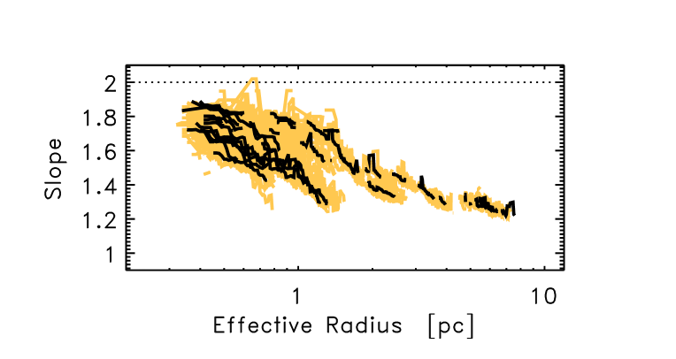
	a) plain differences
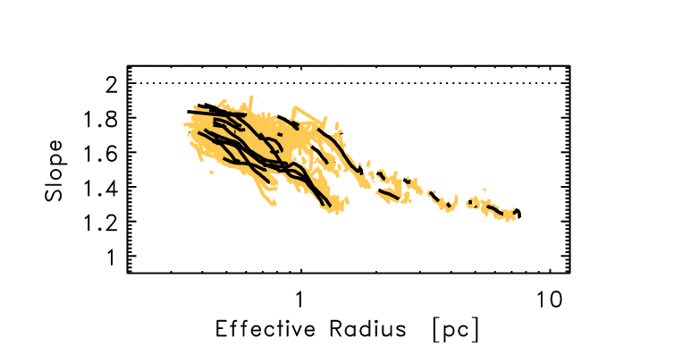
	b) smoothed
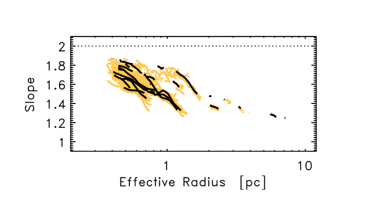
	c) smoothed and filtered

Figure 7.— Calculation scheme for slopes (top to bottom) and impact of noise (black vs. yellow lines). We start with slopes directly calculated from mass and size differences for successive contours (panel a). These measurements are subsequently smoothed (panel b), and data are removed where the smoothing kernel is not filled (panel c). The black lines hold for the observed Perseus extinction data. As in Fig. 5, yellow and black lines indicate results from maps with and without artificial noise, respectively. The dotted line indicates the upper limit on slopes inherent to our method, $b<2$ (Eq. 5).

The impact of noise can be estimated by propagating the mass uncertainties due to noise (Eq. 9) within the slope calculations. This yields

$$\frac{\sigma(b)}{b}\leq 20\,\frac{\sigma(m_{i})}{m}\,\frac{r}{r_{\rm beam}}\,.$$ (15)

Because of the aforementioned smoothing, the numerical constant must be calibrate with our noise experiments (as done for Eq. [9]). To obtain an estimate of the expected uncertainties, we can repeat the mass and size substitutions done in the discussion of Eq. (9). This gives maximum uncertainties $\sim 60\%$. Since $\sigma(b)/b\propto\langle N_{\rm H_{2}}\rangle^{-1}\,r^{-1}$ (see discussion of Eq. [9]), the uncertainties are small for larger regions well above the detection threshold. In practice, uncertainties $<10\%$ are a reasonable estimate for well-detected regions warranting detailed study.

The slope difference due to smoothing is given by the first derivative of the mass bias due to smoothing (Eq. 10) with respect to the radius. Including the usual calibration of numerical constants, we constrain the absolute smoothing-induced error to

$$\Delta b\leq 0.4~{}{\rm to}~{}0.6\,\frac{r_{\rm k}/r}{(1+r_{\rm k}/r)^{3}}\,.$$ (16)

In a few cases, however, the error can be larger by a factor 2. In this paper, we reject regions with a diameter smaller than twice the beam diameter. Substitution of this limit (i.e., $r_{\rm k}/r<1/2$) into Eq. (16) implies that slopes are overestimated by a number smaller than 0.1 due to resolution.

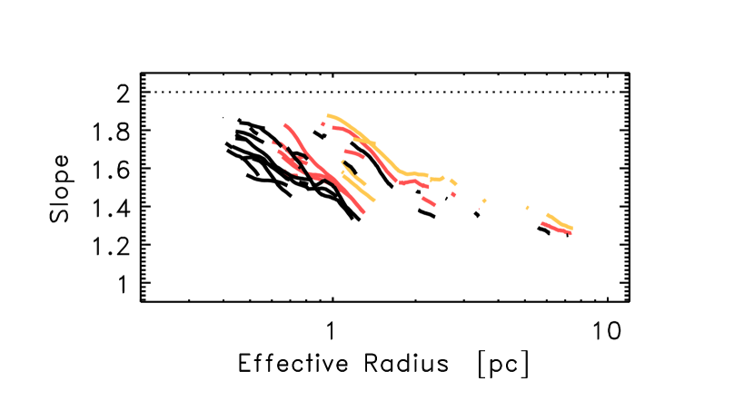
Figure 8.— Impact of limited spatial resolution on slope measurements. See Figs. 5(b) and 7 for explanations of mark-up.

As mentioned in Sec. 4.2.4, bolometer maps suffer from spatial filtering. This has an impact opposite to the influence of smoothing, and artificially shallow slopes are measured from such maps. Since the filtering is very strong in Bolocam maps, we do not use these for the derivation of tangential slopes.

4.4.2 Results for Perseus

Figures 7(c) and 8 show tangential slopes for Perseus. The tangential slopes in the $1\leq r/{\rm pc}\leq 8$ radius interval are in the range $b=1.2~{}{\rm to}~{}1.7$. At a given radius, the slopes for different fragments do often differ by more than their uncertainty. Also, in a given fragment the slope can change significantly with respect to radius. This means that it is not possible to describe an entire cloud by a single tangential slope. The observed tangential slopes bear no obvious relation to the global slope $\sim 1.56$ derived for the same radius range (Fig. 6).

A slope of $\geq 2$ is actually not possible for a mass-size relation as defined by us, since this would require that the column density increases with radius (Eq. 5). Since our search algorithm proceeds by decreasing the column density threshold, such fragments are not identified by our identification scheme. A slope $b<0$ would mean that the mass decreases with increasing radius. This is impossible in all but the most jolly insane models of cloud structure.

5. Summary & Outlook

5.1. Utility of and Outlook for Mass-Size Studies

As we have shown above, our map characterization scheme yields reliable measurements of mass and size. From these, mass-size slopes and intercepts can be derived. Below, we describe how these data contribute to critical fields of star formation research.

First of all, this approach permits a continuous characterization of cloud structure across a large range of spatial scales. This is just a desirable feature of any data analysis method, independent of the exact nature of the later analysis. The need for such a procedure led Rosolowsky et al. (2008b) to the development of the “dendrogram technique”.

In star formation research, the basic mass-size measurements permit to compare fragment masses at a given spatial scale. Consider the classical case in order to see the advantage: usually, “cores” and “clumps” extracted from maps differ in their size. In this case, it is not clear what differences in masses mean, even if just a single cloud is considered.

Spatially continuous cloud characterizations become particularly useful when comparing observations for different molecular clouds. Usually, every cloud is studied at a different physical resolution (i.e., pc per pixel). In the classical case, mass measurements will thus usually refer to vastly different spatial scales. With our approach, however, all scales are probed, and different clouds can be compared at the same physical scale. This is extensively employed in part II, where we study a sample of clouds.

The general utility of measurements of mass and size is known since long. For example, one can compare the actual to virial masses or, more generally, masses predicted by theoretical cloud models. Equation (8), for example, relates model fragment masses and gas temperatures. We shall not discuss such considerations here in detail.

A property uniquely constrained by our method are mass-size slopes; these can only be measured via a scale-independent method. In particular, this gives access to the density structure of molecular clouds. For simple models of cloud structure, the mass-size slope is, e.g., directly related to the slope of the density profile (Eq. 7). Such work on large-scale structure in molecular clouds is urgently needed, since cloud density profiles are presently not known on scales $\gtrsim 0.1~{}\rm pc$. Part II presents slope measurements for various molecular clouds, as well as several model mass-size relations.

5.2. Summary

This work studies the internal structure of molecular clouds by breaking individual cloud complexes up into several nested fragments. For these, we derive masses and sizes, as e.g. outlined in Fig. 1. Effectively, we perform a “dendrogram analysis” of a two-dimensional map, as introduced by Rosolowsky et al. (2008b).

The present paper establishes the method via a detailed analysis of the Perseus Molecular Cloud. Other solar neighborhood molecular clouds ($\lesssim 500~{}\rm pc$; the Pipe Nebula, Taurus, Ophiuchus, and Orion) are discussed in the next paper of this series (part II).

Power-laws of the form $m(r)=m_{0}\,(r/{\rm pc})^{b}$, with slope $b$ and intercept $m_{0}$, prove useful to quantify the relations between mass, $m$, and size, $r$ (i.e., the effective radius). Sections 4.3 and 4.4 discuss two different approaches to define and measure the slope. We use global slopes to measure the relation between structure at small and large scales. This is done by connecting the mass-size measurements of the most massive fragments at small ($0.05~{}\rm pc$) and large radius ($3.0~{}\rm pc$) by a power-law (Eq. 13). Tangential slopes, on the other hand, are calculated infinitesimally at a given spatial scale (Eq. 14). The uncertainties in these properties are examined in Secs. 4.1 and 4.2 (for mass and intercept), respectively Secs. 4.3 and 4.4 (for slopes).

We conclude that our mass, slope, and intercept measurements provide a reliable method to characterize cloud structure. Our approach enables a continuous and reliable characterization of cloud structure in the $0.05\lesssim r/{\rm pc}\lesssim 10$ spatial range. This is not possible using previous methods, since these are usually biased towards a particular spatial scale (see, e.g., the CLUMPFIND analysis in Fig. 4). Such comprehensive pictures of star-forming regions can be used to develop a more complete theoretical understanding of global cloud structure (Sec. 5.1).

A first observational and theoretical exploitation of this method is presented in part II of this series. We characterize, for example, the typical parameter space for solar neighborhood molecular clouds not forming massive stars. Based on this, we chart a potential mass-size threshold for the formation of massive stars. Mass-size slopes are used to constrain large-scale density gradients within molecular clouds.

References

- Ballesteros-Paredes et al. (2007) Ballesteros-Paredes, J., Klessen, R., Mac Low, M.-M., & Vazquez-Semadeni, E. 2007, in Protostars and Planets V, ed. B. Reipurth, D. Jewitt, & K. Keil, 63–80
- Bergin & Tafalla (2007) Bergin, E., & Tafalla, M. 2007, ARA&A, 45, 339
- Bianchi et al. (2003) Bianchi, S., Gonçalves, J., Albrecht, M., Caselli, P., Chini, R., Galli, D., & Walmsley, M. 2003, A&A, 399, L43
- Bohlin et al. (1978) Bohlin, R., Savage, B., & Drake, J. 1978, ApJ, 224, 132
- Cambrésy (1999) Cambrésy, L. 1999, A&A, 345, 965
- Cernis (1993) Cernis, K. 1993, Baltic Astronomy, 2, 214
- Dapp & Basu (2009) Dapp, W., & Basu, S. 2009, MNRAS, 395, 1092
- Enoch et al. (2007) Enoch, M., Glenn, J., Evans II, N., Sargent, A., Young, K., & Huard, T. 2007, ApJ, 666, 982
- Enoch et al. (2006) Enoch, M., Young, K., Glenn, J., Evans II, N., Golwala, S., Sargent, A., Harvey, P., Aguirre, J., Goldin, A., Haig, D., Huard, T., Lange, A., Laurent, G., Maloney, P., Mauskopf, P., Rossinot, P., & Sayers, J. 2006, ApJ, 638, 293
- Goodman et al. (2009a) Goodman, A., Rosolowsky, E., Borkin, M., Foster, J., Halle, M., Kauffmann, J., & Pineda, J. 2009a, Nature, 457, 63
- Goodman et al. (2009b) Goodman, A. A., Pineda, J. E., & Schnee, S. L. 2009b, ApJ, 692, 91
- Hatchell et al. (2005) Hatchell, J., Richer, J., Fuller, G., Qualtrough, C., Ladd, E., & Chandler, C. 2005, A&A, 440, 151
- Johnstone et al. (2000) Johnstone, D., Wilson, C., Moriarty-Schieven, G., Joncas, G., Smith, G., Gregersen, E., & Fich, M. 2000, ApJ, 545, 327
- Kauffmann et al. (2008) Kauffmann, J., Bertoldi, F., Bourke, T., Evans II, N., & Lee, C. 2008, A&A, 487, 993
- Kirk et al. (2006) Kirk, H., Johnstone, D., & Di Francesco, J. 2006, ApJ, 646, 1009
- Larson (1981) Larson, R. 1981, MNRAS, 194, 809
- McKee & Ostriker (2007) McKee, C., & Ostriker, E. 2007, ARA&A, 45, 565
- Motte et al. (1998) Motte, F., Andre, P., & Neri, R. 1998, A&A, 336, 150
- Ossenkopf & Henning (1994) Ossenkopf, V., & Henning, T. 1994, A&A, 291, 943
- Peretto & Fuller (2009) Peretto, N., & Fuller, G. A. 2009, Astronomy and Astrophysics, 505, 405
- Pineda et al. (2009) Pineda, J. E., Rosolowsky, E. W., & Goodman, A. A. 2009, ApJ, 699, L134
- Ridge et al. (2006) Ridge, N., Di Francesco, J., Kirk, H., Li, D., Goodman, A., Alves, J., Arce, H., Borkin, M., Caselli, P., Foster, J., Heyer, M., Johnstone, D., Kosslyn, D., Lombardi, M., Pineda, J., Schnee, S., & Tafalla, M. 2006, AJ, 131, 2921
- Rosolowsky et al. (2008a) Rosolowsky, E., Pineda, J., Foster, J., Borkin, M., Kauffmann, J., Caselli, P., Myers, P., & Goodman, A. 2008a, ApJS, 175, 509
- Rosolowsky et al. (2008b) Rosolowsky, E., Pineda, J., Kauffmann, J., & Goodman, A. 2008b, ApJ, 679, 1338
- Shetty et al. (2010) Shetty, R., Collins, D. C., Kauffmann, J., Goodman, A. A., Rosolowsky, E. W., & Norman, M. L. 2010, eprint arXiv:1001.4549
- Tan (2007) Tan, J. C. 2007, Triggered Star Formation in a Turbulent ISM, 237, 258
- Williams et al. (2000) Williams, J., Blitz, L., & McKee, C. 2000, Protostars and Planets IV, 97
- Williams et al. (1994) Williams, J., de Geus, E., & Blitz, L. 1994, ApJ, 428, 693