Dynamical stability of infinite homogeneous self-gravitating systems: application of the Nyquist method

We complete classical investigations concerning the dynamical stability of an infinite homogeneous gaseous medium described by the Euler-Poisson system or an infinite homogeneous stellar system described by the Vlasov-Poisson system (Jeans problem). To determine the stability of an infinite homogeneous stellar system with respect to a perturbation of wavenumber $k$, we apply the Nyquist method. We first consider the case of single-humped distributions and show that, for infinite homogeneous systems, the onset of instability is the same in a stellar system and in the corresponding barotropic gas, contrary to the case of inhomogeneous systems. We show that this result is true for any symmetric single-humped velocity distribution, not only for the Maxwellian. If we specialize on isothermal and polytropic distributions, analytical expressions for the growth rate, damping rate and pulsation period of the perturbation can be given. Then, we consider the Vlasov stability of symmetric and asymmetric double-humped distributions (two-stream stellar systems) and determine the stability diagrams depending on the degree of asymmetry. We compare these results with the Euler stability of two self-gravitating gaseous streams. Finally, we determine the corresponding stability diagrams in the case of plasmas and compare the results with self-gravitating systems.

1 Introduction

The dynamical stability of self-gravitating systems is an important problem in astrophysics. This problem was first considered by Jeans (1902,1929) who studied the linear dynamical stability of an infinite homogeneous collision-dominated gas described by the Euler equations. He found that this system becomes unstable if the wavelength of the perturbation exceeds a critical value $\lambda_{c}=(\frac{\pi}{G\rho})^{1/2}c_{s}$ (where $c_{s}$ is the velocity of sound) nowadays called the Jeans length. In that case, the perturbation grows exponentially rapidly without oscillating. By contrast, for small wavelengths $\lambda<\lambda_{c}$, the perturbation oscillates without attenuation and behaves like a gravity-modified sound wave. As is well-known, the Jeans approach suffers from a mathematical inconsistency at the start. Indeed, an infinite homogeneous gravitating system cannot be in static equilibrium since there are no pressure gradients to balance the gravitational force. Jeans removed this inconsistency by assuming that the Poisson equation describes only the relationship between the perturbed gravitational potential and the perturbed density. However, this assumption is ad hoc and is known as the Jeans swindle (Binney & Tremaine 1987). A Jeans-type analysis can however be justified in certain situations: (i) In cosmology, when we work in the comoving frame, the expansion of the universe introduces a sort of “neutralizing background” in the Poisson equation (like in the Jellium model of plasma physics). In that case, an infinite homogeneous self-gravitating medium can be in static equilibrium (Peebles 1980). Therefore, the Jeans instability mechanism is relevant to understand the formation of galaxies from the homogeneous early universe. (ii) If we consider a uniformly rotating system, the gravitational attraction can be balanced by the centrifugal force. Therefore, a homogeneous system can be in static equilibrium in the rotating frame provided that the angular velocity and the density satisfy a well-defined relation (Chandrasekhar 1961). (iii) The Jeans procedure is approximately correct if we only consider perturbations with small wavelengths, much smaller than the Jeans length (Binney & Tremaine 1987).

The dynamical stability of an infinite homogeneous encounterless stellar system described by the Vlasov equation was considered much later by Lynden-Bell (1962) who used methods similar to those introduced by Landau (1946) in plasma physics. There exists indeed many analogies between self-gravitating systems and plasmas since the Coulombian and Newtonian interactions both correspond to an inverse square law. However, there exists also crucial differences. First of all, gravity is attractive whereas electricity is repulsive. On the other hand, as already indicated, the self-gravity of a uniform gravitating system is usually not neutralized, contrary to a plasma where the presence of electrons and ions provide electrical neutrality. In order to circumvent the Jeans swindle, Lynden-Bell considered the case of a rotating system and noted that the angular velocity plays a role similar to the magnetic field in plasma physics (Bernstein 1958). He found that the system becomes unstable above a critical wavelength. For a Maxwellian distribution, this critical wavelength $\lambda_{c}=(\frac{\pi}{G\rho})^{1/2}\sigma$ is equivalent to the Jeans length if we identify the r.m.s. velocity of the stars $\sigma$ in one direction with the velocity of sound $c_{s}$ in an isothermal gas. In that case, the perturbation grows exponentially rapidly without oscillating. By contrast, for small wavelengths $\lambda<\lambda_{c}$, the perturbation is damped exponentially. This is similar to the Landau damping in plasma physics that is derived in the complete absence of collisions.

Sweet (1963) considered the gravitational instability of a system of gas and stars in relative motion and provided a detailed analysis of the dispersion relation in different cases. He considered in particular the situation where the gas is at rest ($U=0$) and the star system is made of two identical interpenetrating streams with Maxwellian distribution moving in opposite direction with equal velocity $\pm v_{a}$. This corresponds to the Kapteyn-Eddington two-stream representation in the solar neighborhood. He mentioned that the two humps could be asymmetric but he did not study the consequence of this asymmetry in detail. One important conclusion of his work is that the critical Jeans wavelength is reduced by the relative motion of the gas and stars and that it vanishes when the relative velocity $v_{a}$ exceeds a limit of the order of the effective velocity of sound $c_{s}$ in the gas. In particular, the star streaming in the solar neighborhood can cause the gas to be unstable at all wavelengths. A similar conclusion was reached by Talwar & Kalra (1966) who considered the contrastreaming instability of two self-gravitating gaseous streams with velocity $\pm U$ described by fluid equations. In the subsonic regime $U<c_{s}$, they found that the critical Jeans wavelength is reduced and tends to zero as the streaming velocity $U$ approaches the velocity of sound $c_{s}$ (by contrast, in the supersonic regime $U>c_{s}$, the critical wavelength is larger than the Jeans length without streaming). The works of Sweet (1963) and Talwar & Kalra (1966) were further developed by Ikeuchi et al. (1974) who presented various stability diagrams for two-stream stellar systems, gaseous-stellar systems, two gaseous systems and plasmas. For a purely two-stream stellar systems (without gas), they found that the critical Jeans length becomes larger due to the stabilization effect of relative velocity, contrary to the case where a gas component is present. The two-stream instability was also discussed by Araki (1987) for infinite homogeneous and uniformly rotating stellar systems.

The seminal works of Jeans (for gaseous systems) and Lynden-Bell (for stellar systems) have been continued in several directions. For example, the Jeans instability of a self-gravitating gas in the presence of a magnetic field or an overall rotation has been studied in detail by Chandrasekhar (1961). On the other hand, the gravitational stability of a disk of stars is treated in the classical paper of Toomre (1964). Other interesting contributions are reviewed by Binney & Tremaine (1987). However, this problem is largely academic because real stellar systems (like stars and galaxies) are not spatially homogeneous and are limited in space. Now, when spatial inhomogeneity is properly taken into account, the picture becomes very different. The dynamical stability of stars has been considered by various authors such as Eddington (1918), Ledoux (1945) and Chandrasekhar (1964) and different stability criteria for the Euler-Poisson system have been obtained. For example, it can be shown that polytropic stars are Euler stable if their index $n\leq 3$ while they are unstable if $3<n\leq 5$ (polytropic stars with $n>5$, including isothermal stars $n\rightarrow+\infty$, have infinite mass). On the other hand, the Vlasov stability of stellar systems has been studied by Antonov (1960a), Doremus et al. (1971), Kandrup & Sygnet (1985) and others. They have shown that all stellar systems with a distribution function $f=f(\epsilon)$ which is a monotonically decreasing function of the energy are linearly dynamically stable with respect to the Vlasov-Poisson system. In particular, all polytropic galaxies with index in the range $3/2\leq n\leq 5$ (such that the total mass is finite) are stable. Very recently, it was proven rigorously by Lemou et al. (2009) that these systems are also nonlinearly dynamically stable with respect to the Vlasov-Poisson system. These results show that, when the spatial inhomogeneity of the system is properly accounted for, the Jeans instability is suppressed.

Recently, there was a renewed interest for this classical problem due to analogies with other physical systems. For example, the community of statistical mechanics involved in the dynamics and thermodynamics of systems with long-range interactions (Dauxois et al. 2002) has studied a toy model called the Hamiltonian Mean Field (HMF) model which presents many features similar to self-gravitating systems. In particular, this model presents an instability below a critical temperature that is similar to the Jeans instability in astrophysics. Interestingly, a spatially homogeneous phase exists for this model at any temperature (it is stable for $T>T_{c}$ and unstable for $T<T_{c}$). Therefore, there is no mathematical inconsistency (i.e. no “Jeans swindle”) when we perform the stability analysis of the homogeneous phase of this system (Inagaki & Konishi 1993, Choi & Choi 2003, Yamaguchi et al. 2004, Chavanis & Delfini 2009). On the other hand, in biology, several researchers in physics and applied mathematics have studied the phenomenon of chemotaxis using the Keller-Segel (1970) model in order to explain the self-organization of bacterial colonies, cells or even social insects. Recently, it was shown that the chemotactic instability in biology bears some deep analogies with the Jeans instability in astrophysics (Chavanis 2006b). Interestingly, in the biological problem, there is no “Jeans swindle” because the Poisson equation is replaced by a more complex reaction-diffusion equation that allows for the existence of infinite and homogeneous distributions.

These analogies were a source of motivation to study anew the classical Jeans problem in astrophysics (for the Euler-Poisson and Vlasov-Poisson systems). In fact, we discovered that the study of this classical problem was still incomplete. For example, the case of (spatially homogeneous) polytropic distribution functions has not been investigated in detail and the case of a symmetric double-humped distribution considered by Ikeuchi et al. (1974) needs further discussion. On the other hand, the stability of an asymmetric double-humped distribution has never been considered in the astrophysical literature (although the interest of such distributions was mentioned early by Sweet (1963)) and could form an interesting theoretical problem. The stability criteria for homogeneous stellar systems can be established very easily with the powerful Nyquist method (Nyquist 1932) used in plasma physics. This method can be readily applied to homogeneous self-gravitating systems. However, since the gravitational interaction is attractive while the electric interaction is repulsive, a crucial sign changes in the dispersion relation and the problem must be reconsidered. In particular, this change of sign is the reason for the Jeans instability in astrophysics and the Nyquist method gives a nice graphical illustration of this instability. This method does not seem to be well-known by astrophysicists and is not exposed in classical monographs. Although it essentially has an academic interest since real stellar systems are not spatially homogeneous, we think that it deserves a detailed pedagogical exposition. We thus propose an exhaustive study of the linear dynamical stability of infinite and homogeneous gaseous (Euler) and stellar (Vlasov) systems that uses the Nyquist method and completes previous works on that problem.

The paper is organized as follows. In Sec. 2, we consider a self-gravitating barotropic gas described by the Euler-Poisson system. We recall the classical Jeans instability criterion and, for future comparison, consider explicitly the case of isothermal and polytropic equations of state. In Sec. 3, we consider a collisionless stellar system described by the Vlasov-Poisson system. Using the Nyquist method, we derive the Jeans instability criterion for an infinite and homogeneous distribution. We show that, for any single humped distribution function of the form $f=f(v^{2})$ with $f^{\prime}(v^{2})<0$, the Jeans instability criterion for a stellar system is equivalent to the Jeans instability criterion for the corresponding barotropic gas with the same equation of state. Of course, the dispersion relation and the evolution of the perturbation is different in the two systems (gas and stellar system) but the threshold of the instability is the same. This generalizes the result obtained by Lynden-Bell (1962) for the Maxwellian distribution. In Secs. 4 and 5, we specifically consider the case of isothermal and polytropic distribution functions and derive analytical expressions for the growth rate and damping rate of the perturbation by adapting methods of plasma physics to the gravitational context. In Sec. 6, we consider a symmetric double-humped distribution made of two counter-streaming Maxwellians with velocities $\pm v_{a}$ and establish the stability diagram. In Sec. 7, we generalize our results to the case of an asymmetric double-humped distribution. We find that: (i) The system is stable for $\lambda<(\lambda_{c})_{*}$ and unstable for $\lambda>(\lambda_{c})_{*}$ where the critical wavelength $(\lambda_{c})_{*}$ is a non-trivial function of the relative velocity $v_{a}$ and asymmetry parameter $\Delta$. (ii) The critical wavelength $(\lambda_{c})_{*}$ is always larger than the critical wavelength in the absence of streaming ($v_{a}=0$) so that the instability is delayed. (iii) The phase velocity of the unstable mode corresponds to the global maximum of the distribution function. In Sec. 8, we consider the case of plasmas. We recall the well-known fact that single-humped distributions are always stable. Then, we consider the case of symmetric and asymmetric double-humped distributions. For an asymmetry parameter $\Delta<\Delta_{*}=3.3105$: (i) the system is stable for $v_{a}^{2}<y_{c}(\Delta)T$ where $y_{c}(\Delta)$ depends on the asymmetry ($y_{c}=1.708$ for a symmetric distribution); (ii) for $v_{a}^{2}>y_{c}(\Delta)T$, the system is stable for $\lambda<(\lambda_{c})_{*}$ and unstable for $\lambda>(\lambda_{c})_{*}$ where $(\lambda_{c})_{*}$ depends on the relative velocity $v_{a}$ and on the asymmetry parameter $\Delta$. For an asymmetry parameter $\Delta>\Delta_{*}=3.3105$: (i) the system is stable for $v_{a}^{2}<y_{*}(\Delta)T$ where $y_{*}(\Delta)$ depends on the asymmetry; (ii) for $y_{*}(\Delta)T<v_{a}^{2}<y_{c}(\Delta)T$, the system is stable for $\lambda<(\lambda_{c})_{1}$, unstable for $(\lambda_{c})_{1}<\lambda<(\lambda_{c})_{2}$ and stable for $\lambda>(\lambda_{c})_{2}$ where $(\lambda_{c})_{1}$ and $(\lambda_{c})_{2}$ depend on the relative velocity $v_{a}$ and on the asymmetry parameter $\Delta$; (iii) for $v_{a}^{2}>y_{c}(\Delta)T$, the system is stable for $\lambda<(\lambda_{c})_{1}$ and unstable for $\lambda<(\lambda_{c})_{1}$. Throughout the paper, we also compare our results obtained for stellar systems (Vlasov) to those obtained for gaseous systems (Euler).

2 Self-gravitating barotropic gas

2.1 The Euler-Poisson system

We consider a self-gravitating gas described by the Euler-Poisson system

$${\partial\rho\over\partial t}+\nabla\cdot(\rho{\bf u})=0,$$ (1)

$${\partial{\bf u}\over\partial t}+({\bf u}\cdot\nabla){\bf u}=-{1\over\rho}\nabla p-\nabla\Phi,$$ (2)

$$\Delta\Phi=4\pi G\rho.$$ (3)

These are the usual equations used to study the dynamical stability of a gaseous medium like a molecular cloud or a star. We assume that the gas is a perfect gas in local thermodynamic equilibrium (L.T.E). Therefore, at each point, the distribution function of the particles (atoms or molecules) is of the form

$$f({\bf r},{\bf v},t)=\biggl{[}{1\over 2\pi T({\bf r},t)}\biggr{]}^{3/2}\rho({\bf r},t)e^{-{[{\bf v}-{\bf u}({\bf r},t)]^{2}\over 2T({\bf r},t)}}.$$ (4)

Note that the kinetic temperature $T({\bf r},t)=\frac{1}{3}\langle w^{2}\rangle$ where ${\bf w}={\bf v}-{\bf u}({\bf r},t)$ is the relative velocity. Introducing the pressure $p={1\over 3}\int fw^{2}d{\bf v}$, we find that the local equation of state is

$$p({\bf r},t)=\rho({\bf r},t)T({\bf r},t).$$ (5)

The system of equations (1)-(3) is not closed since it must be supplemented by an equation for the energy or, equivalently, for the temperature $T({\bf r},t)$. Here, we shall restrict ourselves to the case of a barotropic gas for which the pressure depends only on the density

$$p({\bf r},t)=p[\rho({\bf r},t)].$$ (6)

The local velocity of sound is

$$c_{s}^{2}({\bf r},t)=p^{\prime}(\rho({\bf r},t)).$$ (7)

A steady state of the Euler-Poisson system satisfies ${\bf u}={\bf 0}$ and the condition of hydrostatic equilibrium

$$\nabla p+\rho\nabla\Phi={\bf 0}.$$ (8)

Combining the condition of hydrostatic equilibrium (8) and the equation of state $p=p(\rho)$, we find that the density is a function $\rho=\rho(\Phi)$ of the gravitational potential given by

$$\int^{\rho}{p^{\prime}(\rho^{\prime})\over\rho^{\prime}}d\rho^{\prime}=-\Phi.$$ (9)

We note that $p^{\prime}(\rho)=-\rho/\rho^{\prime}(\Phi)$. Since $p^{\prime}(\rho)=c_{s}^{2}\geq 0$, we find that $\rho^{\prime}(\Phi)\leq 0$. The density is a monotonically decreasing function of the gravitational potential. The total energy of the star is

$${\cal W}[\rho,{\bf u}]=\int\rho\int_{0}^{\rho}{p(\rho^{\prime})\over\rho^{{}^{\prime}2}}d\rho^{\prime}d{\bf r}+{1\over 2}\int\rho\Phi d{\bf r}+\int\rho{{\bf u}^{2}\over 2}d{\bf r},$$

(10)

including the internal energy, the potential energy and the kinetic energy of the mean motion. The mass $M[\rho]$ and the energy ${\cal W}[\rho,{\bf u}]$ are conserved by the barotropic Euler-Poisson system: $\dot{M}=\dot{\cal W}=0$. Therefore, a minimum of the energy functional at fixed mass determines a steady state of the barotropic Euler-Poisson system that is nonlinearly dynamically stable. Here, we have stability in the sense of Lyapunov. This means that the size of the perturbation is bounded by the size of the initial perturbation for all times. We are led therefore to considering the minimization problem

$$\min_{\rho,{\bf u}}\ \left\{{\cal W}[\rho]\quad|\quad M[\rho]=M\right\}.$$ (11)

The critical points of energy at fixed mass are determined by the Euler-Lagrange equation $\delta{\cal W}-\mu\delta M=0$ where $\mu$ is a Lagrange multiplier. This yields the condition of hydrostatic equilibrium (8). Then, a critical point of energy at fixed mass is a (local) energy minimum iff

$$\delta^{2}{\cal W}=\int\frac{p^{\prime}(\rho)}{2\rho}(\delta\rho)^{2}\,d{\bf r}+\frac{1}{2}\int\delta\rho\delta\Phi\,d{\bf r}\geq 0$$ (12)

for all perturbations $\delta\rho$ that conserve mass: $\delta M=0$.

2.2 The Jeans instability criterion

We consider the linear dynamical stability of an infinite homogeneous gaseous medium described by the hydrodynamic equations (1), (2), (3) and (6). This is the classical Jeans (1902,1929) problem. Linearizing Eqs. (1)-(3) around a solution $\rho=\Phi={\rm const.}$ and ${\bf u}={\bf 0}$, making the Jeans swindle and decomposing the perturbations in normal modes of the form $e^{i({\bf k}\cdot{\bf r}-\omega t)}$, we obtain the classical dispersion relation (Binney & Tremaine 1987):

$$\omega^{2}=c_{s}^{2}k^{2}-4\pi G\rho,$$ (13)

where $c_{s}^{2}=dp/d\rho$ is the velocity of sound. Since $\omega^{2}$ is real, the complex pulsation $\omega$ is either real or purely imaginary. The condition $\omega=0$ determines a critical wavenumber

$$k_{c}^{2}=\frac{4\pi G\rho}{c_{s}^{2}},$$ (14)

called the Jeans wavenumber for a barotropic gas. The dispersion relation can be rewritten

$$\frac{\omega^{2}}{4\pi G\rho}=\frac{k^{2}}{k_{c}^{2}}-1.$$ (15)

For $k>k_{c}$, we have $\omega=\omega_{r}=\pm\sqrt{\omega^{2}}$ so that the perturbation oscillates like $e^{-i\omega_{r}t}$ with a pulsation

$$\omega_{r}=\pm\sqrt{c_{s}^{2}k^{2}-4\pi G\rho},$$ (16)

without attenuation. This corresponds to gravity-modified sound waves. In that case the system is stable. For $k<k_{c}$, we have $\omega=\omega_{i}=\pm i\sqrt{-\omega^{2}}$ so that the perturbation grows like $e^{\omega_{i}t}$ with a growth rate

$$\omega_{i}=\sqrt{4\pi G\rho-c_{s}^{2}k^{2}},$$ (17)

without oscillation (the second mode is attenuated exponentially rapidly so that the growing mode dominates). In that case, the system is unstable. This is the so-called Jeans instability. The growth rate is maximum for $k=0$ and its value is $\omega_{i}(k=0)=\sqrt{4\pi G\rho}$.

In conclusion, a perturbation with wavenumber $k$ is stable if

$$k>k_{c}=\frac{\sqrt{4\pi G\rho}}{c_{s}},$$ (18)

and unstable otherwise. These results are valid for an arbitrary barotropic equation of state $p=p(\rho)$. We now specialize on particular cases, namely isothermal and polytropic equations of state.

2.3 Isothermal equation of state

We first consider an isothermal equation of state

$$p({\bf r},t)=\rho({\bf r},t)T,$$ (19)

where the temperature $T({\bf r},t)=T$ is a uniform. At hydrostatic equilibrium, according to Eq. (9), the relation between the density and the gravitational potential is given by the Boltzmann law

$$\rho=A^{\prime}e^{-{\Phi\over T}},$$ (20)

where $A^{\prime}$ is a constant. The energy functional (10) reads

$${\cal W}[\rho,{\bf u}]=k_{B}T\int{\rho}\ln{\rho}d{\bf r}+{1\over 2}\int\rho\Phi d{\bf r}+\int\rho{{\bf u}^{2}\over 2}d{\bf r},$$

(21)

and it can be viewed as a Boltzmann free energy $F=E-TS$ where $E$ is the macroscopic energy and $S$ the Boltzmann entropy. The velocity of sound (7) is uniform:

$$c_{s}^{2}=T.$$ (22)

Finally, for an infinite homogeneous isothermal gas, the Jeans instability criterion takes the classical form

$$k^{2}<k^{2}_{c}=\frac{4\pi G\rho}{T}.$$ (23)

2.4 Polytropic equation of state

The equation of state of a polytropic gas is

$$p({\bf r},t)=K\rho({\bf r},t)^{\gamma},$$ (24)

where $K$ is a constant. The polytropic index $n$ is defined by $\gamma=1+1/n$. For $n\rightarrow+\infty$, we recover the isothermal case with $\gamma=1$. At hydrostatic equilibrium, according to Eq. (9), the relation between the density and the gravitational potential can be written

$$\rho=\biggl{[}\lambda-{\gamma-1\over K\gamma}\Phi\biggr{]}^{1\over\gamma-1},$$ (25)

where $\lambda$ is a constant. The energy functional (10) can be put in the form

$${\cal W}[\rho,{\bf u}]={K\over\gamma-1}\int(\rho^{\gamma}-\rho)d{\bf r}+{1\over 2}\int\rho\Phi d{\bf r}+\int\rho{{\bf u}^{2}\over 2}d{\bf r}.$$

(26)

In the limit $\gamma\rightarrow 1$, we recover the results (20) and (21) obtained for isothermal distributions. For a polytropic gas, the local temperature $T({\bf r},t)$ given by Eq. (5) reads

$$T({\bf r},t)=K\rho({\bf r},t)^{\gamma-1}.$$ (27)

We note that the temperature is position dependent (while the specific entropy $s$ is uniform) and related to the density by a power law (this is the local version of the usual isentropic law $TV^{\gamma-1}={\rm const.}$ in thermodynamics). The polytropic index $n$ is related to the gradients of temperature and density according to

$${\nabla\ln T}={1\over n}\nabla\ln\rho.$$ (28)

Combining Eqs. (25) and (27), we note that, for a polytropic gas at equilibrium, the relation between the kinetic temperature and the gravitational potential is linear so that

$$\nabla T=-\frac{\gamma-1}{\gamma}\nabla\Phi.$$ (29)

The coefficient of proportionality is related to the adiabatic index $\gamma$. The velocity of sound (7) can be expressed as

$$c_{s}({\bf r},t)^{2}=\gamma T({\bf r},t),$$ (30)

and it is usually position dependent. However, when we consider an infinite and homogeneous distribution (making the Jeans swindle), the velocity of sound and the temperature are uniform. In that case, we can speak of “the temperature $T$ of the polytropic gas” and write the Jeans instability criterion as

$$k^{2}<k^{2}_{c}=\frac{4\pi G\rho}{\gamma T}.$$ (31)

We thus find that the critical Jeans wavenumber $k_{c}^{(poly)}$ of a polytropic gas is related to the critical Jeans wavenumber $k_{c}^{(iso)}$ of an isothermal gas with the same temperature $T$ by

$$k_{c}^{(poly)}=\frac{1}{\sqrt{\gamma}}k_{c}^{(iso)},$$ (32)

where the proportionality factor is the polytropic index $\gamma$. The positivity of $c_{s}^{2}=dp/d\rho$ implies that $\gamma\geq 0$, i.e. $n\geq 0$ or $n\leq-1$ (for $-1<n<0$, the gas is always unstable, even in the absence of gravity, since $\omega^{2}<0$). For $\gamma=0$ ($n=-1$), the gas is unstable to all wavelengths since $k_{c}^{(poly)}=+\infty$. For $0<\gamma<1$ ($n<-1$), $k_{c}^{(poly)}>k_{c}^{(iso)}$. For $\gamma=1$ ($n=\infty$), $k_{c}^{(poly)}=k_{c}^{(iso)}$ (isothermal case). For $\gamma>1$ ($n>0$), $k_{c}^{(poly)}<k_{c}^{(iso)}$. For $\gamma=+\infty$ ($n=0$), the gas is stable to all wavelengths since $k_{c}^{(poly)}=0$ (solid medium). For an isentropic gas for which $\gamma=c_{p}/c_{v}$, the Mayer relation $c_{p}-c_{v}=k_{B}$ implies that $\gamma>1$ ($n>0$). Therefore, for an isentropic gas, the gravitational instability is always delayed (i.e., it occurs for larger wavelengths) with respect to an isothermal gas with the same temperature.

3 Collisionless stellar systems

3.1 The Vlasov-Poisson system

We consider a self-gravitating system described by the Vlasov-Poisson system

$${\partial f\over\partial t}+{\bf v}\cdot{\partial f\over\partial{\bf r}}+{\bf F}\cdot{\partial f\over\partial{\bf v}}=0,$$ (33)

$$\Delta\Phi=4\pi G\int fd{\bf v},$$ (34)

where ${\bf F}=-\nabla\Phi$ is the self-consistent gravitational field produced by the particles. The Vlasov description assumes that the evolution of the system is encounterless. This is a very good approximation for most astrophysical systems like galaxies and dark matter because the relaxation time due to close encounters is in general larger than the age of the universe by several orders of magnitude (Binney & Tremaine 1987). The Vlasov equation admits an infinite number of stationary solutions given by the Jeans theorem (Jeans 1915). For example, distribution functions of the form $f=f(\epsilon)$ which depend only on the individual energy $\epsilon={v^{2}}/{2}+\Phi({\bf r})$ of the stars are particular steady states of the Vlasov equation. They describe spherical stellar systems.

The Vlasov equation conserves the mass $M[f]=\int f\,d{\bf r}d{\bf v}$, the energy $E[f]=\frac{1}{2}\int fv^{2}\,d{\bf r}d{\bf v}+\frac{1}{2}\int\rho\Phi\,d{\bf r}$ and the Casimirs $I_{h}=\int h(f)\,d{\bf r}d{\bf v}$ for any continuous function $h$. Let us introduce the functionals

$$S=-\int C(f)\,d{\bf r}d{\bf v},$$ (35)

where $C$ is a convex function ($C^{\prime\prime}>0$). These particular Casimirs will be called “pseudo entropies”.

The two constraints problem: since the Vlasov equation conserves $M$, $E$ and $S$, the maximization problem

$$\max_{f}\ \left\{S[f]\quad|\quad E[f]=E,\quad M[f]=M\right\},$$ (36)

determines a steady state of the Vlasov-Poisson system that is nonlinearly dynamically stable. The critical points of pseudo entropy at fixed mass and energy are determined by the variational principle $\delta S-\beta\delta E-\alpha\delta M=0$, where $\beta$ (pseudo inverse temperature) and $\alpha$ (pseudo chemical potential) are Lagrange multipliers. This yields $C^{\prime}(f)=-\beta\epsilon-\alpha$. Since $C$ is convex, this relation can be reversed to give $f=F(\beta\epsilon+\alpha)$ where $F=(C^{\prime})^{-1}(-x)$. We have $f^{\prime}(\epsilon)=-\beta/C^{\prime\prime}(f)$. Therefore, if $\beta>0$, the critical points of pseudo entropy at fixed mass and energy determine distributions of the form $f=f(\epsilon)$ with $f^{\prime}(\epsilon)<0$: the distribution function is a monotonically decreasing function of the energy. Then, a critical point of pseudo entropy at fixed mass and energy is a (local) maximum iff

$$\delta^{2}{S}=-\frac{1}{2}\int C^{\prime\prime}(f)(\delta f)^{2}\,d{\bf r}d{\bf v}-\frac{1}{2}\beta\int\delta\rho\delta\Phi\,d{\bf r}<0,$$ (37)

for all perturbations $\delta f$ that conserve mass and energy at first order: $\delta M=\delta E=0$.

The one constraint problem: the minimization problem

$$\min_{f}\ \left\{F[f]=E[f]-TS[f]\quad|\quad M[f]=M\right\},$$ (38)

where $T=1/\beta>0$ is prescribed, determines a steady state of the Vlasov-Poisson system that is nonlinearly dynamically stable. The functional $F[f]$ is a pseudo free energy. The critical points of pseudo free energy at fixed mass are determined by the variational principle $\delta F+\alpha T\delta M=0$, where $\alpha$ (pseudo chemical potential) is a Lagrange multiplier. This yields $C^{\prime}(f)=-\beta\epsilon-\alpha$. Then, a critical point of pseudo free energy at fixed mass is a (local) minimum iff

$$\delta^{2}{F}=\frac{1}{2}T\int C^{\prime\prime}(f)(\delta f)^{2}\,d{\bf r}d{\bf v}+\frac{1}{2}\int\delta\rho\delta\Phi\,d{\bf r}>0,$$ (39)

for all perturbations $\delta f$ that conserve mass: $\delta M=0$.

The no constraint problem: the maximization problem

$$\max_{f}\ \left\{G[f]=S[f]-\beta E[f]-\alpha M[f]\right\},$$ (40)

where $\beta$ and $\alpha$ are prescribed, determines a steady state of the Vlasov-Poisson system that is nonlinearly dynamically stable. The functional $G[f]$ is a pseudo grand potential. The critical points of pseudo grand potential $G$, satisfying $\delta G=0$, are given by $C^{\prime}(f)=-\beta\epsilon-\alpha$. Then, a critical point of pseudo grand potential is a (local) maximum iff

$$\delta^{2}{G}=-\frac{1}{2}\int C^{\prime\prime}(f)(\delta f)^{2}\,d{\bf r}d{\bf v}-\frac{1}{2}\beta\int\delta\rho\delta\Phi\,d{\bf r}<0,$$ (41)

for all perturbations $\delta f$.

The optimization problems (36), (38) and (40) have the same critical points (canceling the first order variations). Furthermore, a solution of (40) is always a solution of the more constrained dual problem (38). Indeed, if inequality (41) is true for all perturbations, it is true a fortiori for all perturbations that conserve mass. Similarly, a solution of (38) is always a solution of the more constrained dual problem (36). Indeed, if inequality (39) is true for all perturbations that conserve mass, it is true a fortiori for all perturbations that conserve mass and energy. However, the reciprocal is wrong. A solution of (38) is not necessarily a solution of (40), and a solution of (36) is not necessarily a solution of (38). This is similar to the notion of ensemble inequivalence in thermodynamics (Ellis et al. 2000, Bouchet & Barré 2005, Chavanis 2006a). Indeed, the two constraints problem (36) is similar to a condition of microcanonical stability, the one constraint problem (38) is similar to a condition of canonical stability, and the no constraint problem (40) is similar to a condition of grand canonical stability. The implication $(\ref{erica1})\Rightarrow(\ref{vh4})\Rightarrow(\ref{vh3})$ is similar to the fact that grand canonical stability implies canonical stability which itself implies microcanonical stability (but not the converse) in thermodynamics. Therefore, (40) provides just a sufficient condition of nonlinear dynamical stability that is less refined than (38), and (38) provides just a sufficient condition of nonlinear dynamical stability that is less refined than (36).

The most refined problem: the minimization problem

$$\min_{f}\ \left\{E[f]\quad|{\rm\ all\ the\ Casimirs\ }I_{h}\right\},$$ (42)

determines a steady state of the Vlasov-Poisson system that is nonlinearly dynamically stable. A distribution function is a critical point of energy for symplectic perturbations (i.e. perturbations that conserve all the Casimirs) iff $f({\bf r},{\bf v})$ is a steady state of the Vlasov equation (Bartholomew 1971, Kandrup 1991). Furthermore, if we consider spherical stellar systems for which $f=f(\epsilon)$, it can be shown (Bartholomew 1971, Kandrup 1991) that a critical point of energy for symplectic perturbations is a (local) minimum iff

$$\delta^{2}{E}=-\frac{1}{2}\int\frac{(\delta f)^{2}}{f^{\prime}(\epsilon)}\,d{\bf r}d{\bf v}+\frac{1}{2}\int\delta\rho\delta\Phi\,d{\bf r}>0,$$ (43)

for all perturbations $\delta f$ that conserve energy and all the Casimirs at first order: $\delta E=\delta I_{h}=0$. Such symplectic (physically accessible) perturbations are of the form $\delta f=D\delta g$ where $D={\bf v}\cdot\nabla_{\bf r}-\nabla\Phi\cdot\nabla_{\bf v}$ is the advective operator in phase space and $\delta g({\bf r},{\bf v})$ is any perturbation. Inequality (43) corresponds to the Antonov (1960) criterion of dynamical stability that was obtained by investigating the linear dynamical stability of a steady state of the Vlasov equation. Since this is the most constrained criterion, this is the most refined one. We note that inequality (43) is equivalent to inequalities (37), (39) and (41) if we use the identity $f^{\prime}(\epsilon)=-\beta/C^{\prime\prime}(f)$ derived above. However, the classes of perturbations to consider are different: in (41), we must consider all perturbations, in (39) we must consider perturbations that conserve mass, in (37) we must consider perturbations that conserve mass and energy, and in (43) we must consider perturbations that conserve energy and all the Casimirs. Therefore, we have the implications $(\ref{erica1})\Rightarrow(\ref{vh4})\Rightarrow(\ref{vh3})\Rightarrow(\ref{erica3})$. The connection between (42) and the preceding optimization problems can be understood as follows. The minimization problem (42), conserving all the Casimirs, is clearly more refined than the minimization problem

$$\min_{f}\ \left\{E[f]\quad|\quad M[f]=M,\quad S[f]=S\right\},$$ (44)

where only the mass and one Casimir of the form (35) is conserved. Now, it is easy to show that the minimization problem (44) is equivalent to the maximization problem (36). Hence, we have the chain of relations

$$(\ref{erica1})\Rightarrow(\ref{vh4})\Rightarrow(\ref{vh3})\Leftrightarrow(\ref{erica5})\Rightarrow(\ref{erica3}).$$ (45)

To summarize, the minimization problem (42) is the most refined stability criterion because it tells that, in order to settle the dynamical stability of a stellar system, we just need considering symplectic (i.e. dynamically accessible) perturbations. Of course, if inequality (43) is satisfied by a larger class of perturbations, as implied by problems (40), (38), (36) and (44), the system will be stable a fortiori. Therefore, we have the implications (45). Problems (40), (38), (36) and (44) provide sufficient (but not necessary) conditions of dynamical stability. A steady state can be stable according to (38) while it does not satisfy (40), or it can be stable according to (36) and (44) while it does not satisfy (38), or it can be stable according to (42) while it does not satisfy (36) and (44). Therefore, the criterion (42) is more refined than (44) or (36), which is itself more refined than (38), which is itself more refined than (40). Let us give an astrophysical illustration of all that (Chavanis 2006a). Using (38), we can show that stellar polytropes with $3/2\leq n\leq 3$ are dynamically stable because they are minima of $F$ at fixed mass $M$. By contrast, stellar polytropes with $3<n<5$ are not minima of $F$ at fixed mass. However, using (36), we can show that stellar polytropes with $3/2<n<5$ are dynamically stable because they are maxima of $S$ at fixed mass and energy. However, not all stellar systems of the form $f=f(\epsilon)$ are maxima of $S$ at fixed mass and energy. But, using (42), we can show that all spherical galaxies $f=f(\epsilon)$ with $f^{\prime}(\epsilon)<0$ are dynamically stable. This last statement has been shown for linear stability by Kandrup (1991). A rigorous mathematical proof has been given recently by Lemou et al. (2009) for nonlinear stability.

Remark: similar results are obtained in 2D fluid mechanics based on the Euler-Poisson system (see Chavanis 2009). Criterion (42) is equivalent to the so-called Kelvin-Arnol’d energy principle, criterion (40) is equivalent to the standard Casimir-energy method (see Holm et al. 1985) introduced by Arnol’d (1966) and criterion (36) is equivalent to the refined stability criterion given by Ellis et al. (2002).

3.2 The corresponding barotropic star

To any stellar system with $f=f(\epsilon)$ and $f^{\prime}(\epsilon)<0$, we can associate a corresponding barotropic star with the same equilibrium density distribution (Lynden-Bell & Sanitt 1969). Indeed, defining the density and the pressure by $\rho=\int fd{\bf v}$ and $p={1\over 3}\int fv^{2}d{\bf v}$, we get $\rho=\rho(\Phi)$ and $p=p(\Phi)$. Eliminating the potential $\Phi$ between these two expressions, we find that $p=p(\rho)$. Furthermore, taking the gradient of the pressure and using the chain of identities

$$\nabla p={1\over 3}\int{\partial f\over\partial{\bf r}}v^{2}d{\bf v}={1\over 3}\nabla\Phi\int f^{\prime}(\epsilon)v^{2}d{\bf v}$$

$$={1\over 3}\nabla\Phi\int{\partial f\over\partial{\bf v}}\cdot{\bf v}\,d{\bf v}=-\nabla\Phi\int f\,d{\bf v}=-\rho\nabla\Phi,$$ (46)

we obtain the condition of hydrostatic equilibrium (8). Finally, we define the kinetic temperature of an isotropic stellar system by the relation

$$\frac{3}{2}T({\bf r})=\frac{1}{2}\langle v^{2}\rangle.$$ (47)

Therefore, the quantity

$$T({\bf r})=\frac{1}{3}\langle v^{2}\rangle={{1\over 3}\int fv^{2}d{\bf v}\over\int fd{\bf v}}={p({\bf r})\over\rho({\bf r})}.$$ (48)

measures the velocity dispersion (in one direction) of an isotropic stellar system. In general, the kinetic temperature is position dependent.

Finally, we can show that the variational principles $(\ref{vh4})$ and $(\ref{ep10})$ are equivalent, i.e. a stellar system is a minimum of pseudo free energy at fixed mass iff the corresponding barotropic gas is a minimum of energy at fixed mass (see Appendix A). This leads to a nonlinear version of the Antonov (1960b) first law: “a stellar system with $f=f(\epsilon)$ and $f^{\prime}(\epsilon)<0$ is nonlinearly dynamically stable with respect to the Vlasov-Poisson system if the corresponding barotropic gas is nonlinearly dynamically stable with respect to the Euler-Poisson system”. However, the reciprocal is wrong because, as we have already indicated, (38) provides just a sufficient condition of nonlinear dynamical stability with respect to the Vlasov equation. A galaxy can be dynamically stable according to criterion (36) [or even more generally (42)] while it fails to satisfy criterion (38). Therefore, the nonlinear Antonov first law is similar to a notion of ensembles inequivalence between microcanonical and canonical ensembles in thermodynamics (Chavanis 2006a).

3.3 The dispersion relation

We shall study the linear dynamical stability of a spatially homogeneous stationary solution of the Vlasov equation described by a distribution function $f=f({\bf v})$. Like for an infinite homogeneous gas, we make the Jeans swindle. Linearizing the Vlasov equation around this steady state, taking the Laplace-Fourier transform of this equation and writing the perturbations in the form $e^{i({\bf k}\cdot{\bf r}-\omega t)}$, we obtain the classical dispersion relation (Binney & Tremaine 1987):

$$\epsilon({\bf k},\omega)\equiv 1+{4\pi G\over k^{2}}\int{{\bf k}\cdot{\partial f\over\partial{\bf v}}\over{\bf k}\cdot{\bf v}-\omega}d{\bf v}=0,$$ (49)

where $\epsilon({\bf k},\omega)$ is similar to the “dielectric function” of plasma physics (with the sign $+$ instead of $-$). For a given distribution $f({\bf v})$, this equation determines the complex pulsation(s) $\omega=\omega_{r}+i\omega_{i}$ of a perturbation with wavevector ${\bf k}$. Since the time dependence of the perturbation is $\delta f\sim e^{-i\omega_{r}t}e^{\omega_{i}t}$, the system is linearly stable if $\omega_{i}<0$ and linearly unstable if $\omega_{i}>0$. The condition of marginal stability corresponds to $\omega_{i}=0$.

If we take the wavevector ${\bf k}$ along the $z$-axis, the dispersion relation becomes

$$\epsilon({k},\omega)\equiv 1+{4\pi G\over k^{2}}\int_{C}{{k}{\partial f\over\partial{v_{z}}}\over{k}{v_{z}}-\omega}d{v}_{x}d{v}_{y}d{v}_{z}=0,$$ (50)

where the integral must be performed along the Landau contour $C$ (Binney & Tremaine 1987). We define

$$g(v_{z})=\int fdv_{x}dv_{y}.$$ (51)

In the following, we shall note $v$ instead of $v_{z}$ and $f$ instead of $g$. With these conventions, the dispersion relation (50) can be rewritten

$$\epsilon({k},\omega)\equiv 1+{4\pi G\over k^{2}}\int_{C}{f^{\prime}(v)\over{v}-\frac{\omega}{k}}d{v}=0.$$ (52)

This is the fundamental equation of the problem. For future reference, let us recall that

$$\int_{C}{{f^{\prime}(v)}\over v-\frac{\omega}{k}}dv=\int_{-\infty}^{+\infty}{{f^{\prime}(v)}\over v-\frac{\omega}{k}}dv,\quad(\omega_{i}>0),$$ (53)

$$\int_{C}{{f^{\prime}(v)}\over v-\frac{\omega}{k}}dv=P\int_{-\infty}^{+\infty}{{f^{\prime}(v)}\over v-\frac{\omega}{k}}dv+i\pi f^{\prime}\left(\frac{\omega}{k}\right),\quad(\omega_{i}=0),$$

(54)

$$\int_{C}{{f^{\prime}(v)}\over v-\frac{\omega}{k}}dv=\int_{-\infty}^{+\infty}{{f^{\prime}(v)}\over v-\frac{\omega}{k}}dv+2\pi if^{\prime}\left(\frac{\omega}{k}\right),\quad(\omega_{i}<0),$$

(55)

where $P$ denotes the principal value.

In general, the dispersion relation (52) cannot be solved explicitly to obtain $\omega(k)$ except in some very simple cases . For example, for cold systems described by the distribution function $f=\rho\delta({v}-{v}_{0})$, we obtain after an integration by parts

$$\omega=v_{0}k\pm i\sqrt{4\pi G\rho}.$$ (56)

In particular, when $v_{0}=0$, we get

$$\omega=\pm i\sqrt{4\pi G\rho}.$$ (57)

The system is unstable to all wavenumbers and the perturbation grows with a growth rate $\omega_{i}=\sqrt{4\pi G\rho}$. We also note that the dispersion relation (57) coincides with the dispersion relation (17) of a self-gravitating gas with $c_{s}=0$.

3.4 The condition of marginal stability

For $\omega_{i}=0$, the real and imaginary parts of the dielectric function $\epsilon(k,\omega_{r})=\epsilon_{r}(k,\omega_{r})+i\epsilon_{i}(k,\omega_{r})$ are given by

$$\epsilon_{r}({k},\omega_{r})=1+\frac{4\pi G}{k^{2}}P\int_{-\infty}^{+\infty}{f^{\prime}(v)\over{v}-{\omega_{r}}/{k}}d{v},$$ (58)

$$\epsilon_{i}({k},\omega_{r})=\frac{4\pi^{2}G}{k^{2}}f^{\prime}\left({\omega_{r}}/{k}\right).$$ (59)

The condition of marginal stability corresponds to $\epsilon(k,\omega)=0$ and $\omega_{i}=0$, i.e. $\epsilon_{r}({k},\omega_{r})=\epsilon_{i}({k},\omega_{r})=0$. We obtain therefore the equations

$$1+\frac{4\pi G}{k^{2}}P\int_{-\infty}^{+\infty}{f^{\prime}(v)\over{v}-{\omega_{r}}/{k}}d{v}=0,$$ (60)

$$f^{\prime}\left({\omega_{r}}/{k}\right)=0.$$ (61)

The second condition (61) imposes that the phase velocity $\omega_{r}/k=v_{ext}$ is equal to a velocity where $f(v)$ is extremum ($f^{\prime}(v_{ext})=0$). The first condition (60) then determines the wavenumber(s) $k_{c}$ corresponding to marginal stability. It can be written

$$1+\frac{4\pi G}{k_{c}^{2}}\int_{-\infty}^{+\infty}{f^{\prime}(v)\over{v}-v_{ext}}d{v}=0,$$ (62)

where the principal value is not needed anymore. The wavenumber(s) corresponding to marginal stability are therefore given by

$$k_{c}=\left(-4\pi G\int_{-\infty}^{+\infty}\frac{f^{\prime}(v)}{v-v_{ext}}\,dv\right)^{1/2}.$$ (63)

Finally, the pulsation(s) corresponding to marginal stability are $\omega_{r}=v_{ext}k_{c}$ and we have $\delta f\sim e^{-i\omega_{r}t}$. Note that the distribution $f(v)$ can be relatively arbitrary. There can be pure oscillations ($\omega=\omega_{r}\neq 0$) only if $f(v)$ has some extrema at $v\neq 0$. If $f(v)$ has a single maximum at $v=0$, then $\omega_{r}=0$ (implying $\omega=0$) and the condition of marginal stability becomes

$$k_{c}=\left(-4\pi G\int_{-\infty}^{+\infty}\frac{f^{\prime}(v)}{v}\,dv\right)^{1/2}.$$ (64)

3.5 The Nyquist method

To determine whether the distribution $f=f(v)$ is stable or unstable for a perturbation with wavenumber $k$, one possibility is to solve the dispersion relation (52) and determine the sign of the imaginary part of the complex pulsation. This can be done analytically in some simple cases (see Secs. 3.8, 4 and 5). We can also apply the Nyquist method introduced in plasma physics. This is a graphical method that does not require to solve the dispersion relation. The details of the method are explained by Nicholson (1992) and we just recall how it works in practice. In the $\epsilon$-plane, taking $\omega_{i}=0$, we plot the Nyquist curve $(\epsilon_{r}(k,\omega_{r}),\epsilon_{i}(k,\omega_{r}))$ parameterized by $\omega_{r}$ going from $-\infty$ to $+\infty$ (for a given wavenumber $k$). This curve is closed and always rotates in the counterclockwise sense. If the Nyquist curve does not encircle the origin, the system is stable (for the corresponding wavenumber $k$). If the Nyquist curve encircles the origin one or more times, the system is unstable. The number $N$ of tours around the origin gives the number of zeros of $\epsilon(k,\omega)$ in the upper half $\omega$-plane, i.e. the number of unstable modes with $\omega_{i}>0$. The Nyquist method by itself does not give the growth rate of the instability.

Let us consider the asymptotic behavior of $(\epsilon_{r}(k,\omega_{r}),\epsilon_{i}(k,\omega_{r}))$ defined by Eqs. (58) and (59) for $\omega_{r}\rightarrow\pm\infty$. Since $f(v)$ is positive and tends to zero for $v\rightarrow\pm\infty$, we conclude that $\epsilon_{i}(k,\omega_{r})\rightarrow 0$ for $\omega_{r}\rightarrow\pm\infty$ and that $\epsilon_{i}(k,\omega_{r})>0$ for $\omega_{r}\rightarrow-\infty$ while $\epsilon_{i}(k,\omega_{r})<0$ for $\omega_{r}\rightarrow+\infty$. On the other hand, integrating by parts in Eq. (58), we obtain

$$\epsilon_{r}(k,\omega_{r})=1+\frac{4\pi G}{k^{2}}{P}\int_{-\infty}^{+\infty}{{f(v)}\over(v-\omega_{r}/k)^{2}}dv,$$ (65)

provided that $f(v)$ decreases sufficiently rapidly. Therefore, for $\omega_{r}\rightarrow\pm\infty$, we obtain at leading order

$$\epsilon_{r}(k,\omega_{r})\simeq 1+\frac{4\pi G\rho}{\omega_{r}^{2}},\qquad(\omega_{r}\rightarrow\pm\infty).$$ (66)

In particular, $\epsilon_{r}(k,\omega_{r})\rightarrow 1^{+}$ for $\omega_{r}\rightarrow\pm\infty$. From these results, we conclude that the behavior of the Nyquist curve close to the limit point $(1,0)$ is like the one represented in Fig. 3. In addition, according to Eq. (59), the Nyquist curve crosses the $x$-axis at each value of $\omega_{r}/k$ corresponding to an extremum of $f(v)$. For $\omega_{r}/k=v_{ext}$, where $v_{ext}$ is a velocity at which the distribution is extremum $(f^{\prime}(v_{ext})=0)$, the imaginary part of the dielectric function $\epsilon_{i}(k,kv_{ext})=0$ and the real part of the dielectric function

$$\epsilon_{r}(k,kv_{ext})=1+\frac{4\pi G}{k^{2}}\int_{-\infty}^{\infty}\frac{f^{\prime}(v)}{v-v_{ext}}\,dv.$$ (67)

Subtracting the value $f^{\prime}(v_{ext})=0$ in the numerator of the integrand, and integrating by parts, we obtain

$$\epsilon_{r}(k,kv_{ext})=1-\frac{4\pi G}{k^{2}}\int_{-\infty}^{\infty}\frac{f(v_{ext})-f(v)}{(v-v_{ext})^{2}}\,dv.$$ (68)

If $v_{Max}$ denotes the velocity corresponding to the global maximum of the distribution, we clearly have

$$\epsilon_{r}(k,kv_{Max})=1-\frac{4\pi G}{k^{2}}\int_{-\infty}^{\infty}\frac{f(v_{Max})-f(v)}{(v-v_{Max})^{2}}\,dv<1.$$

(69)

Furthermore, $\epsilon_{r}(k,kv_{Max})<0$ for sufficiently small $k$. Therefore, by tuning $k$ appropriately, we can always make the Nyquist curve encircle the origin. We conclude that a spatially homogeneous self-gravitating system is always unstable to some wavelengths.

3.6 Single-humped distributions

Let us assume that the distribution $f(v)$ has a single maximum at $v=v_{0}$ (so that $f^{\prime}(v_{0})=0$) and tends to zero for $v\rightarrow\pm\infty$. Then, the Nyquist curve cuts the $x$-axis ($\epsilon_{i}(k,\omega_{r})$ vanishes) at the limit point $(1,0)$ where $\omega_{r}\rightarrow\pm\infty$ and at the point $(\epsilon_{r}(k,kv_{0}),0)$ where $\omega_{r}/k=v_{0}$. Due to its behavior close to the limit point $(1,0)$, the fact that it rotates in the counterclockwise sense, and the property that $\epsilon_{r}(k,kv_{0})<1$ according to Eq. (69), the Nyquist curve must necessarily behave like in Fig. 3. Therefore, the Nyquist curve starts on the real axis at $\epsilon_{r}(k,\omega_{r})=1$ for $\omega_{r}\rightarrow-\infty$, then going in counterclockwise sense it crosses the real axis at the point $\epsilon_{r}(k,kv_{0})<1$ and returns on the real axis at $\epsilon_{r}(k,\omega_{r})=1$ for $\omega_{r}\rightarrow+\infty$. According to the Nyquist criterion exposed in Sec. 3.5, we conclude that a single-humped distribution is linearly stable with respect to a perturbation with wavenumber $k$ if

$$\epsilon_{r}(k,kv_{0})=1+\frac{4\pi G}{k^{2}}\int_{-\infty}^{+\infty}{{f^{\prime}(v)}\over v-v_{0}}dv>0,$$ (70)

and linearly unstable if $\epsilon_{r}(k,kv_{0})<0$. The equality corresponds to the marginal stability condition (62). Therefore, the system is stable iff

$$k>k_{c}=\left(-4\pi G\int_{-\infty}^{+\infty}\frac{f^{\prime}(v)}{v-v_{0}}\,dv\right)^{1/2},$$ (71)

where $k_{c}$ is the critical Jeans wavenumber for a stellar system. Note that an infinite homogeneous stellar system whose DF has a single hump is always unstable to sufficiently small wavenumbers. For the unstable wavenumbers $k<k_{c}$, there is only one mode of instability $\omega_{i}>0$ since the Nyquist curve rotates only one time around the origin. This stability criterion is valid for any single-humped distribution. In particular, a symmetric distribution $f=f(v)$ with a single maximum at $v_{0}=0$ is linearly dynamically stable to a perturbation with wavenumber $k$ iff

$$k>k_{c}=\left(-4\pi G\int_{-\infty}^{+\infty}\frac{f^{\prime}(v)}{v}\,dv\right)^{1/2}.$$ (72)

We shall make the connection between the stability of an infinite homogeneous stellar system and the stability of the corresponding barotropic gas in Sec. 3.9. In particular, using identity (96), we will show that Eq. (72) is equivalent to Eq. (18).

3.7 Double-humped distributions

Let us consider a double-humped distribution with a global maximum at $v_{Max}$, a minimum at $v_{min}$ and a local maximum at $v_{max}$. We assume that $v_{Max}<v_{min}<v_{max}$. The Nyquist curve will cut the $x$-axis at the limit point $(1,0)$ and at three other points $(\epsilon_{r}(k,kv_{Max}),0)$, $(\epsilon_{r}(k,kv_{min}),0)$ and $(\epsilon_{r}(k,kv_{max}),0)$. We also know that the Nyquist curve can only rotate in the counterclockwise sense and that $\epsilon_{r}(k,kv_{Max})<1$ according to Eq. (69). Then, we can convince ourselves, by making drawings, of the following results. If

$(+++)$: $\epsilon_{r}(v_{Max})>0$, $\epsilon_{r}(v_{min})>0$, $\epsilon_{r}(v_{max})>0$,

$(+--)$: $\epsilon_{r}(v_{Max})>0$, $\epsilon_{r}(v_{min})<0$, $\epsilon_{r}(v_{max})<0$,

$(--+)$: $\epsilon_{r}(v_{Max})<0$, $\epsilon_{r}(v_{min})<0$, $\epsilon_{r}(v_{max})>0$,

$(+-+)$ : $\epsilon_{r}(v_{Max})>0$, $\epsilon_{r}(v_{min})<0$, $\epsilon_{r}(v_{max})>0$,

the Nyquist curve does not encircle the origin so the system is stable. If

$(---)$: $\epsilon_{r}(v_{Max})<0$, $\epsilon_{r}(v_{min})<0$, $\epsilon_{r}(v_{max})<0$,

$(-++)$: $\epsilon_{r}(v_{Max})<0$, $\epsilon_{r}(v_{min})>0$, $\epsilon_{r}(v_{max})>0$,

$(++-)$: $\epsilon_{r}(v_{Max})>0$, $\epsilon_{r}(v_{min})>0$, $\epsilon_{r}(v_{max})<0$,

the Nyquist curve rotates one time around the origin so that there is one mode of instability. Finally, if

$(-+-)$: $\epsilon_{r}(v_{Max})<0$, $\epsilon_{r}(v_{min})>0$, $\epsilon_{r}(v_{max})<0$,

the Nyquist curve rotates two times around the origin so that there are two modes of instability. Cases $(+++)$, $(---)$, $(-++)$ and $(-+-)$ are observed in Sec. 7 for an asymmetric double-humped distribution made of two Maxwellians. The other cases cannot be obtained from this distribution but they may be obtained from other distributions.

If the double-humped distribution is symmetric with respect to the origin with two maxima at $\pm v_{*}$ and a minimum at $v=0$, only three cases can arise. If

$(+++)$: $\epsilon_{r}(v_{*})>0$, $\epsilon_{r}(0)>0$,

$(+-+)$: $\epsilon_{r}(v_{*})>0$, $\epsilon_{r}(0)<0$,

the Nyquist curve does not encircle the origin so the system is stable. If

$(---)$: $\epsilon_{r}(v_{*})<0$, $\epsilon_{r}(0)<0$,

the Nyquist curve rotates one time around the origin so that there is one mode of instability. Finally, if

$(-+-)$: $\epsilon_{r}(v_{*})<0$, $\epsilon_{r}(0)>0$,

the Nyquist curve rotates two times around the origin so that there are two modes of instability. Cases $(+++)$, $(---)$ and $(-+-)$ are observed in Sec. 3.1 for a symmetric double-humped distribution made of two Maxwellians.

3.8 Particular solutions of $\epsilon(k,\omega)=0$

We can look for a solution of the dispersion relation $\epsilon(k,\omega)=0$ in the form $\omega=i\omega_{i}$ corresponding to $\omega_{r}=0$. In that case, the perturbation grows ($\omega_{i}>0$) or decays ($\omega_{i}<0$) without oscillating. For $\omega_{i}>0$, the equation $\epsilon(k,\omega)=0$ becomes

$$1+{4\pi G\over k^{2}}\int_{-\infty}^{+\infty}\frac{f^{\prime}(v)}{v-i\frac{\omega_{i}}{k}}\,dv=0.$$ (73)

Multiplying the numerator by $v+i\omega_{i}/k$ and separating real and imaginary parts, we obtain

$$1+{4\pi G\over k^{2}}\int_{-\infty}^{+\infty}\frac{vf^{\prime}(v)}{v^{2}+\frac{\omega_{i}^{2}}{k^{2}}}\,dv=0,$$ (74)

$$\int_{-\infty}^{+\infty}\frac{f^{\prime}(v)}{v^{2}+\frac{\omega_{i}^{2}}{k^{2}}}\,dv=0.$$ (75)

If we consider distribution functions $f(v)$ that are symmetric with respect to $v=0$, Eq. (75) is always satisfied. Then, the growth rate $\omega_{i}>0$ is given by Eq. (74).

For $\omega_{i}<0$, the equation $\epsilon(k,\omega)=0$ becomes

$$1+{4\pi G\over k^{2}}\int_{-\infty}^{+\infty}\frac{f^{\prime}(v)}{v-i\frac{\omega_{i}}{k}}\,dv+i\frac{8\pi^{2}G}{k^{2}}f^{\prime}\left(\frac{i\omega_{i}}{k}\right)=0.$$ (76)

Multiplying the numerator by $v+i\omega_{i}/k$ and assuming that $f(v)$ is even, we obtain

$$1+{4\pi G\over k^{2}}\int_{-\infty}^{+\infty}\frac{vf^{\prime}(v)}{v^{2}+\frac{\omega_{i}^{2}}{k^{2}}}\,dv+i\frac{8\pi^{2}G}{k^{2}}f^{\prime}\left(\frac{i\omega_{i}}{k}\right)=0,$$ (77)

which determines the damping rate $\omega_{i}<0$.

Let us introduce the function $K(x)$ defined by

$$K(x)=\frac{1}{I}\int_{-\infty}^{+\infty}\frac{vf^{\prime}(v)}{v^{2}+x^{2}}\,dv\ (x\geq 0)$$ (78)

$$K(x)=\frac{1}{I}\left\{\int_{-\infty}^{+\infty}\frac{vf^{\prime}(v)}{v^{2}+x^{2}}\,dv+2\pi if^{\prime}(ix)\right\}\ (x\leq 0)$$ (79)

where

$$I=\int_{-\infty}^{+\infty}\frac{f^{\prime}(v)}{v}\,dv.$$ (80)

This function is normalized such that $K(0)=1$. The dispersion relations (74) and (77) can then be written

$$1-\frac{k_{c}^{2}}{k^{2}}K\left(\frac{\omega_{i}}{k}\right)=0,$$ (81)

where $k_{c}$ is the maginal wavenumber corresponding to $\omega=0$ given by Eq. (64). The pulsation $\omega_{i}(k)$ is given by

$$\frac{\omega_{i}}{k_{c}}=\frac{k}{k_{c}}K^{-1}\left(\frac{k^{2}}{k_{c}^{2}}\right).$$ (82)

Setting $u=\omega_{i}/k$, it can also be written in parametric form as

$$\frac{\omega_{i}}{k_{c}}=u\sqrt{K(u)},\qquad\frac{k}{k_{c}}=\sqrt{K(u)},$$ (83)

where $u$ goes from $-\infty$ to $+\infty$.

Let us obtain some asymptotic expansions of these relations (valid for symmetric distributions):

(i) Let us first consider the case $\omega_{i}>0$ and $k\rightarrow 0$ corresponding to instability. Integrating Eq. (74) by parts, we obtain

$$1-4\pi G\int_{-\infty}^{+\infty}\frac{f(v)(\omega_{i}^{2}-k^{2}v^{2})}{(k^{2}v^{2}+\omega_{i}^{2})^{2}}\,dv=0.$$ (84)

Expanding the integrand in powers of $kv/\omega_{i}\ll 1$, we find that

$$\omega_{i}^{2}=4\pi G\rho-3Tk^{2}-...\qquad(k\rightarrow 0),$$ (85)

with $T=\langle v^{2}\rangle$ (where we recall that $v=v_{z}$ in the present case). This expression can be compared with the corresponding expression (306) valid for a gas. This identification yields $c_{s}^{2}=3T$ so that large wavelength perturbations in a collisionless stellar system correspond to one dimensional isentropic perturbations with index $\gamma=3$ in a gas (see Appendix B).

(ii) The case $\omega_{i}<0$ and $k\rightarrow+\infty$ corresponding to stability cannot be treated at a general level because the result depends on the behavior of the distribution function for large velocities. The case of a Maxwellian distribution is specifically considered in Sec. 4.

(iii) Let us finally consider the behavior of the dispersion relation (74) or (77) close to the point of marginal stability $k=k_{c}$. For $\omega_{i}=0$, we obtain the critical wavenumber $k_{c}$ given by Eq. (64). Let us consider $\omega_{i}\rightarrow 0^{+}$ and $k\rightarrow k_{c}^{-}$ in Eq. (74). We introduce the function

$$F(x)=\int_{-\infty}^{+\infty}\frac{vf^{\prime}(v)}{v^{2}+x^{2}}\,dv,$$ (86)

for any real $x$. For $x\rightarrow 0$, we have the Taylor expansion $F(x)=F(0)+F^{\prime}(0)x+...$ with

$$F(0)=\int_{-\infty}^{+\infty}\frac{f^{\prime}(v)}{v}\,dv,$$ (87)

$$F^{\prime}(x)=-\int_{-\infty}^{+\infty}\frac{2xvf^{\prime}(v)}{(v^{2}+x^{2})^{2}}\,dv=-\int_{-\infty}^{+\infty}\frac{xf^{\prime\prime}(v)}{v^{2}+x^{2}}\,dv,$$

(88)

where we have used an integration by parts to get the last expression. Under this form, we cannot take the limit $x\rightarrow 0$ in the integral because the integral is not convergent for $x=0$. However, if we write Eq. (88) in the equivalent form

$$F^{\prime}(x)=-x\int_{-\infty}^{+\infty}\frac{f^{\prime\prime}(v)-f^{\prime\prime}(0)}{v^{2}+x^{2}}\,dv-\int_{-\infty}^{+\infty}\frac{xf^{\prime\prime}(0)}{v^{2}+x^{2}}\,dv,$$

(89)

we obtain

$$F^{\prime}(0)=-\lim_{x\rightarrow 0}xf^{\prime\prime}(0)\int_{-\infty}^{+\infty}\frac{dv}{v^{2}+x^{2}}=-\pi f^{\prime\prime}(0){\rm sign}(x).$$

(90)

Regrouping the previous results, we find that the dispersion relation (74) becomes for $\omega_{i}\rightarrow 0^{+}$:

$$1+\frac{4\pi G}{k^{2}}\left\{\int_{-\infty}^{+\infty}\frac{f^{\prime}(v)}{v}\,dv-\pi f^{\prime\prime}(0)\frac{\omega_{i}}{k}\right\}=0.$$ (91)

Similarly, the dispersion relation (77) becomes for $\omega_{i}\rightarrow 0^{-}$:

$$1+\frac{4\pi G}{k^{2}}\left\{\int_{-\infty}^{+\infty}\frac{f^{\prime}(v)}{v}\,dv+\pi f^{\prime\prime}(0)\frac{\omega_{i}}{k}\right\}$$

$$-\frac{8\pi^{2}G}{k^{2}}f^{\prime\prime}(0)\frac{\omega_{i}}{k}=0,$$ (92)

which takes the same form as Eq. (91). Therefore, Eq. (91) is valid for $\omega_{i}\rightarrow 0$ whatever its sign. To leading order, we obtain

$$\omega_{i}=\frac{-k_{c}^{3}}{4\pi^{2}Gf^{\prime\prime}(0)}\left(1-\frac{k^{2}}{k_{c}^{2}}\right),\qquad(k\rightarrow k_{c}).$$ (93)

This formula leads to the following result. First of all, we recall that the mode of marginal stability that we consider corresponds to $\omega_{r}/k=v_{ext}=0$, i.e. to the extremum value of the distribution function $f(v)$ at $v_{ext}=0$. If the distribution is maximum at $v=0$, so that $f^{\prime\prime}(0)<0$, we find that the mode $\omega=i\omega_{i}$ is stable for $k>k_{c}$ and unstable for $k<k_{c}$. Alternatively, if the distribution is minimum at $v=0$, so that $f^{\prime\prime}(0)>0$, we find that the mode $\omega=i\omega_{i}$ is stable for $k<k_{c}$ and unstable for $k>k_{c}$. This result will be illustrated in connection to Fig. 10 for the symmetric double humped distribution.

In this section, we have discussed particular solutions of the dispersion relation of the form $\omega=i\omega_{i}$. Of course, there may exist other solutions to the equation $\epsilon(k,\omega)=0$ with $\omega_{r}\neq 0$. However, for single-humped distributions and unstable wavenumbers $k<k_{c}$, the Nyquist curve encircles the origin only once (see Sec. 3.6) so that, when it exists, the solution $\omega=i\omega_{i}$ with $\omega_{i}>0$ is the only solution of $\epsilon(k,\omega)=0$ (for single-humped distributions and stable wavenumbers $k>k_{c}$, there may exist other solutions of $\epsilon(k,\omega)=0$ with $\omega_{r}\neq 0$ and $\omega_{i}<0$ as discussed in Sec. 4.4). Explicit solutions of the dispersion relation $\epsilon(k,\omega)=0$ with $\omega=i\omega_{i}$ are given in Secs. 4 and 5 for isothermal and polytropic distributions.

3.9 Equivalence between the Jeans instability criterion for a stellar system and the Jeans instability criterion for the corresponding barotropic gas

Lynden-Bell (1962) first observed that the critical Jeans length for a stellar system described by a Maxwellian distribution function is equal to the critical Jeans length for an isothermal gas if we replace the velocity of sound by the velocity dispersion in one direction. In this section, we provide the appropriate generalization of this result for an arbitrary distribution of the form $f=f(v^{2})$ with $f^{\prime}<0$.

As indicated in Sec. 3.2, to any stellar system with a distribution function $f=f(\epsilon)$ and $f^{\prime}(\epsilon)<0$, we can associate a corresponding barotropic gas with an equation of state $p=p(\rho)$. According to Eq. (9), the condition of hydrostatic equilibrium can be written

$$p^{\prime}(\rho)=-\frac{\rho}{\rho^{\prime}(\Phi)}.$$ (94)

Now, using Eq. (7) and the fact that $\rho=\int f(\epsilon)\,d{\bf v}$, we get

$$c_{s}^{2}({\bf r})=-\frac{\rho({\bf r})}{\int f^{\prime}(\epsilon)\,d{\bf v}}=-\frac{\rho({\bf r})}{\int\frac{\frac{\partial f}{\partial v_{z}}}{v_{z}}d{\bf v}}=-\frac{\rho({\bf r})}{\int_{-\infty}^{+\infty}\frac{\frac{\partial g}{\partial v_{z}}}{v_{z}}d{v}_{z}},$$

(95)

where $g({\bf r},v_{z})=\int f(\epsilon)\,dv_{x}dv_{y}$. For a spatially homogeneous system, we obtain the identity

$$c_{s}^{2}=-\frac{\rho}{\int_{-\infty}^{+\infty}\frac{f^{\prime}(v)}{v}\,d{v}},$$ (96)

where we have noted $v$ for $v_{z}$ and $f$ for $g$ like in Sec. 3.3. This identity is explicitly checked in Appendix C for the isothermal and polytropic distributions. Since $f(v)$ is symmetric with respect to $v=0$ and has a single maximum at $v=0$, the Jeans instability criterion can be written (see Sec. 3.6):

$$k^{2}<k_{c}^{2}=-4\pi G\int_{-\infty}^{+\infty}\frac{f^{\prime}(v)}{v}\,dv.$$ (97)

Using identity (96), it can be rewritten

$$k^{2}<k_{c}^{2}=\frac{4\pi G\rho}{c_{s}^{2}}.$$ (98)

Therefore, the criterion of dynamical stability for a spatially homogeneous stellar system coincides with the criterion of dynamical stability for the corresponding barotropic gas (see Sec. 2.2). We insist on the fact that this equivalence is valid for an arbitrary distribution function of the form $f=f(v^{2})$ with $f^{\prime}<0$, not only for the Maxwellian. We conclude that: an infinite homogeneous stellar system with $f=f(v^{2})$ and $f^{\prime}<0$ is dynamically stable with respect to a perturbation with wavenumber $k$ if and only if the corresponding barotropic gas is dynamically stable with respect to this perturbation. This is the proper formulation of the Antonov first law for spatially homogeneous systems: in the present case, we have equivalence. Of course, although the thresholds of stability/instability coincide, the evolution of the perturbation is different in a stellar system and in a fluid system (see Secs. 4 and 5). We should also emphasize that, in general, the velocity of sound $c_{s}$ in the corresponding barotropic gas is not equal to the velocity dispersion $\langle v^{2}\rangle^{1/2}$ in the stellar system, except when $f(v)$ is the Maxwellian distribution leading to Lynden-Bell’s result.

4 Isothermal stellar systems

4.1 The equation of state

We consider an isothermal stellar system described by the distribution function

$$f=Ae^{-\beta\epsilon},$$ (99)

where $\beta=1/T$ is a pseudo inverse temperature. We justify here this distribution as a particular steady state of the Vlasov equation. The associated pseudo entropy is

$$S[f]=-\int f\ln(f/f_{0})d{\bf r}d{\bf v},$$ (100)

where $f_{0}$ is a constant introduced to make the term in the logarithm dimensionless (it will play no role in the following since it appears in an additional constant term). The distribution (99) is obtained by extremizing the pseudo entropy (100) at fixed mass and energy, writing $\delta S-\beta\delta E-\alpha\delta M=0$. For an isothermal distribution, the kinetic temperature (velocity dispersion) defined by Eq. (48) is spatially uniform, and it coincides with the pseudo temperature: $T({\bf r})=T$. The barotropic gas corresponding to the isothermal stellar system defined by Eq. (99) is the isothermal gas with an equation of state $p({\bf r})=\rho({\bf r})T$. The velocity of sound is also spatially uniform and it coincides with the velocity dispersion in one direction: $c_{s}^{2}({\bf r})=T$. The density is related to the gravitational potential by Eq. (20). It can be obtained by integrating Eq. (99) on the velocities leading to Eq. (20) with $A^{\prime}=A(2\pi/\beta)^{3/2}$. It can also be obtained by using Eq. (9) with $p({\bf r})=\rho({\bf r})T$, or by extremizing the functional (21) at fixed mass (Chavanis 2006a). Finally, combining Eqs (99) and (20), we can express the distribution function in terms of the density profile according to

$$f=\biggl{(}{\beta\over 2\pi}\biggr{)}^{3/2}\rho({\bf r})\ e^{-\beta{v^{2}\over 2}}.$$ (101)

Remark: the stability of box-confined isothermal stellar systems has been studied by Antonov (1962), Lynden-Bell & Wood (1968), Padmanabhan (1990) and Chavanis (2006a).

4.2 The dispersion relation

Let us now consider an infinite homogeneous isothermal system described by the Maxwellian distribution function (101) with uniform density $\rho({\bf r})=\rho$. The reduced distribution (51) is

$$f=\biggl{(}{\beta\over 2\pi}\biggr{)}^{1/2}\rho\ e^{-\beta{v^{2}\over 2}}.$$ (102)

The Maxwellian distribution has a single maximum at $v=0$. Therefore, the condition of marginal stability (61) implies $\omega_{r}=0$. From Eq. (60), we find that the Maxwellian distribution is marginally stable for $k=k_{c}$ where we have introduced the critical wavenumber

$$k_{c}^{2}=\frac{4\pi G\rho}{T}.$$ (103)

According to the criterion (71), the Maxwell distribution is linearly dynamically stable if $k>k_{c}$ and linearly dynamically unstable if $k<k_{c}$. The critical Jeans wavenumber (103) for an isothermal stellar system is the same as the critical Jeans wavenumber (23) for an isothermal gas. This is to be expected on account of the general result of Sec. 3.9.

The dielectric function (52) associated to the Maxwellian distribution is

$$\epsilon(k,\omega)=1-\frac{4\pi G}{k^{2}}\left(\frac{\beta}{2\pi}\right)^{1/2}\rho\int_{C}\frac{\beta v}{v-\frac{\omega}{k}}e^{-\beta{v^{2}\over 2}}\ dv.$$ (104)

Introducing the critical Jeans wavenumber (103), it can be rewritten

$$\epsilon({k},\omega)=1-{k_{c}^{2}\over k^{2}}W\biggl{(}{\sqrt{\beta}\omega\over k}\biggr{)},$$ (105)

where

$$W(z)={1\over\sqrt{2\pi}}\int_{C}{x\over x-z}e^{-{x^{2}\over 2}}dx,$$ (106)

is the $W$-function of plasma physics (Ichimaru 1973). We note that $W(0)=1$. For any complex number $z$, we have the analytical expression

$$W(z)=1-ze^{-{z^{2}\over 2}}\int_{0}^{z}e^{x^{2}\over 2}\,dx+i{\sqrt{\pi\over 2}}ze^{-{z^{2}\over 2}}.$$ (107)

4.3 Growth rate and damping rate

We look for particular solutions of the dispersion relation $\epsilon({k},\omega)=0$ in the form $\omega=i\omega_{i}$ where $\omega_{i}$ is real. Using Eq. (107), we note that

$$\epsilon({k},i\omega_{i})=1-{k_{c}^{2}\over k^{2}}H\biggl{(}\frac{\sqrt{\beta}\omega_{i}}{k}\biggr{)},$$ (108)

where we have introduced the function

$$H(x)\equiv W(ix)=1-\sqrt{\frac{\pi}{2}}xe^{\frac{x^{2}}{2}}{\rm erfc}\left(\frac{x}{\sqrt{2}}\right).$$ (109)

This function has the following asymptotic behaviors: (i) For $x\rightarrow 0$, $H(x)=1-\sqrt{\frac{\pi}{2}}x+...$. (ii) For $x\rightarrow+\infty$, $H(x)=\frac{1}{x^{2}}(1-{3\over x^{2}}+...)$. (iii) For $x\rightarrow-\infty$, $H(x)\sim-\sqrt{2\pi}xe^{\frac{x^{2}}{2}}$ (see Fig. 1). Using $\epsilon(k,i\omega_{i})=0$, the relation between $\omega_{i}$ and $k$ (for fixed $T$) can be written

$$1-{k_{c}^{2}\over k^{2}}H\biggl{(}{\sqrt{\beta}\omega_{i}\over k}\biggr{)}=0,$$ (110)

or more explicitly

$$1-{k_{c}^{2}\over k^{2}}\biggl{\{}1-\sqrt{\pi\beta\over 2}{\omega_{i}\over k}e^{{\beta\omega_{i}^{2}\over 2k^{2}}}{\rm erfc}\biggl{(}\sqrt{\frac{\beta}{2}}{\omega_{i}\over k}\biggr{)}\biggr{\}}=0.$$ (111)

This equation can also be obtained directly from Eqs. (53) and (55) (see Appendix D). If we set $x=\sqrt{\beta}\omega_{i}/k$, we can rewrite Eq. (110) in the parametric form

$$\frac{\omega_{i}}{\sqrt{4\pi G\rho}}=x\sqrt{H(x)},\qquad\frac{k^{2}}{k_{c}^{2}}={H(x)}.$$ (112)

By varying $x$ between $-\infty$ and $+\infty$, we obtain the full curve giving $\omega_{i}$ as a function of the wavenumber $k$ (see Fig. 2). Since the time dependence of the perturbation is $\delta f\sim e^{\omega_{i}t}$, the case of neutral stability $\omega_{i}=0$ corresponds to $k=k_{c}$, the case of instability $\omega_{i}>0$ corresponds to $k<k_{c}$ and the case of stability $\omega_{i}<0$ corresponds to $k>k_{c}$. We have the asymptotic behaviors

$${\omega_{i}\over\sqrt{4\pi G\rho}}\sim 1-\frac{3}{2}{k^{2}\over k_{c}^{2}},\qquad(k/k_{c}\rightarrow 0),$$ (113)

$${\omega_{i}\over\sqrt{4\pi G\rho}}\sim\sqrt{\frac{2}{\pi}}\biggl{(}1-{k^{2}\over k_{c}^{2}}\biggr{)},\qquad(k/k_{c}\rightarrow 1),$$ (114)

$${\omega_{i}\over\sqrt{4\pi G\rho}}\sim-\sqrt{{2k^{2}\over k_{c}^{2}}\ln\biggl{(}{k^{2}\over k_{c}^{2}}\biggr{)}},\qquad(k/k_{c}\rightarrow+\infty).$$ (115)

Figure 1: The function $H(x)$.

Figure 2: Pulsation $\omega$ as a function of the wavenumber $k$ for an isothermal stellar system. For $k<k_{J}$, the system is unstable and $\omega=i\omega_{i}$ with $\omega_{i}>0$. For $k>k_{J}$, the system is stable. There exists many branches of solutions $\omega=\omega_{r}+i\omega_{i}$ with $\omega_{i}<0$ (see Sec. 4.4) but we have only represented the branch corresponding to $\omega_{r}=0$. We have also compared these results with the case of an isothermal gas. For $k<k_{J}$, the system is unstable and $\omega=\pm i\omega_{i}$. For $k>k_{J}$, the system is stable and $\omega=\pm\omega_{r}$.

Equation (112) provides a particular solution of the dispersion relation $\epsilon(k,\omega)=0$ of the form $\omega=i\omega_{i}$ with $\omega_{r}=0$. The dispersion relation may have other solutions with $\omega_{r}\neq 0$. However, for single humped distributions, we know that there is only one unstable mode with $\omega_{i}>0$ for given $k<k_{c}$ (see Sec. 3.6). Since the solutions $\omega=i\omega_{i}$ given by Eq. (112) exist for any $k<k_{c}$, we conclude that they are the only solutions in that range of wavenumbers. Therefore, for the unstable wavenumbers $k<k_{c}$, the perturbation grows exponentially rapidly without oscillating. In other words, there are no overstable modes for the Maxwell distribution. This is the same behavior as in a fluid system (see Sec. 2) except that the growth rate $\omega_{i}>0$ in the stellar system [see Eq. (112)] and in the fluid system [see Eq. (17)] are different. For the stable wavenumbers $k>k_{c}$, the perturbations in a stellar system are damped exponentially rapidly ($\omega_{i}<0$). We have exhibited particular solutions (112) that are damped without oscillating $\omega_{r}=0$ but these are not the only solutions of the dispersion relation. There also exists modes that are damped exponentially ($\omega_{i}<0$) and oscillate $\omega_{r}\neq 0$ (see asymptotic results in Sec. 4.4). This form of damping for collisionless stellar systems is similar to the Landau damping for a plasma. The situation is very different in a fluid system. In that case, the stable modes with wavenumbers $k>k_{c}$ correspond to gravity-modified sound waves that propagate without attenuation ($\omega_{r}\neq 0$, $\omega_{i}=0$).

The pulsation of the perturbations in an infinite homogeneous isothermal stellar system is plotted in Fig. 2 as a function of the wavenumber $k$. For comparison, we have also indicated the pulsation of the perturbations in an infinite homogeneous isothermal gas.

4.4 Other branches for $k\rightarrow+\infty$

Let us solve the dispersion relation $\epsilon(k,\omega)=0$ for an isothermal distribution in the limit $k\rightarrow+\infty$. We look for a solution of the equation $\epsilon(k,\omega)=0$ of the form $\omega=\omega_{r}+i\omega_{i}$ with $\omega_{i}<0$ (damping) and $\omega_{i}\gg\omega_{r}$. This corresponds to heavily damped perturbations. We shall check this approximation a posteriori. Using Eq. (55) for $\omega_{i}<0$ , Eq. (52) can be written

$$1+\frac{4\pi G}{k^{2}}\int_{-\infty}^{+\infty}{{f^{\prime}(v)}\over v-\frac{\omega}{k}}\,dv+\frac{8\pi^{2}G}{k^{2}}if^{\prime}\left(\frac{\omega}{k}\right)=0.$$ (116)

If $f(v)$ decreases like $e^{-\beta v^{2}/2}$ for real $v\rightarrow\pm\infty$, then for complex $\omega=\omega_{r}+i\omega_{i}$ with $\omega_{i}\gg\omega_{r}$, $f^{\prime}(\omega/k)$ will increase like $e^{\beta\omega_{i}^{2}/2k^{2}}$. Therefore, to leading order, the foregoing equation reduces to

$$1+\frac{8\pi^{2}G}{k^{2}}if^{\prime}\left(\frac{\omega}{k}\right)=0.$$ (117)

Separating real and imaginary parts, we obtain two transcendant equations

$${\rm Re}\left[\frac{8\pi^{2}G}{k^{2}}if^{\prime}\left(\frac{\omega_{r}+i\omega_{i}}{k}\right)\right]=-1,$$ (118)

$${\rm Im}\left[if^{\prime}\left(\frac{\omega_{r}+i\omega_{i}}{k}\right)\right]=0,$$ (119)

which crucially depend on the form of the distribution. For the Maxwellian (102), they can be rewritten to leading order in the limit $\omega_{i}/\omega_{r}\gg 1$ as

$$\frac{8\pi^{2}G}{k^{3}}\left(\frac{\beta}{2\pi}\right)^{1/2}\rho\beta\omega_{i}e^{\frac{\beta\omega_{i}^{2}}{2k^{2}}}\cos\left(\frac{\beta\omega_{r}\omega_{i}}{k^{2}}\right)=-1,$$ (120)

$$\sin\left(\frac{\beta\omega_{r}\omega_{i}}{k^{2}}\right)=0.$$ (121)

Equation (121) implies $\beta\omega_{r}\omega_{i}/k^{2}=m\pi$. Eq. (120) will have a solution provided that $m$ is even. Then, Eq. (120) gives

$$\frac{8\pi^{2}G}{k^{3}}\left(\frac{\beta}{2\pi}\right)^{1/2}\rho\beta\omega_{i}e^{\frac{\beta\omega_{i}^{2}}{2k^{2}}}=-1,$$ (122)

which determines $\omega_{i}$. By a graphical construction, it is easy to see that $|\omega_{i}|$ is an increasing function of $k$. For $k\rightarrow+\infty$, we find the asymptotic behaviors

$$\omega_{i}=-\frac{2}{\sqrt{\beta}}k\sqrt{\ln k},\qquad\omega_{r}=-m\frac{\pi}{2}\frac{1}{\sqrt{\beta}}\frac{k}{\sqrt{\ln k}}.$$ (123)

Since $\omega_{i}/\omega_{r}\sim\ln k\rightarrow+\infty$, our basic assumption is satisfied. Therefore, for $k>k_{c}$ we have several branches of solutions parameterized by the even integer $m$. For $m=0$, we recover the results of Sec. 4.3.

Remark: by analogy with plasma physics, we could also look for solutions of the dispersion relation (52) of the form $\omega=\omega_{r}+i\omega_{i}$ with $\omega_{i}\ll\omega_{r}$. This corresponds to weakly damped perturbations. In plasma physics, these solutions are valid for $k\rightarrow 0$ and lead to the usual Landau damping formula. However, a self-gravitating system is unstable for $k<k_{c}$. Furthermore, it is easy to show that there is no solution of that form to Eq. (52) whatever the form of the distribution $f(v)$ and the wavenumber $k$. This implies that for attractive interactions (like gravity) the perturbations are unstable for $k<k_{c}$ and heavily damped for $k>k_{c}$ while for repulsive interaction (like plasmas) they are weakly damped for $k<k_{D}$ and heavily damped for $k>k_{D}$.

4.5 Nyquist curve

It will be convenient in the following to work with dimensionless quantities. We introduce the dimensionless wavenumber and the dimensionless pulsation

$$\eta=\frac{4\pi G\rho}{Tk^{2}},\qquad\Omega=\frac{\omega}{\sqrt{4\pi G\rho}},$$ (124)

Noting that $\sqrt{\beta}\omega/k=\sqrt{\eta}\Omega$, the dielectric function (105) can be rewritten

$$\epsilon({\eta},\Omega)=1-\eta W(\sqrt{\eta}\Omega).$$ (125)

When $\Omega_{i}=0$, the real and imaginary parts of the dielectric function $\epsilon(\eta,\Omega_{r})=\epsilon_{r}(\eta,\Omega_{r})+i\epsilon_{i}(\eta,\Omega_{r})$ can be written

$$\epsilon_{r}(\eta,\Omega_{r})=1-\eta W_{r}\left(\sqrt{\eta}\Omega_{r}\right),$$ (126)

$$\epsilon_{i}(\eta,\Omega_{r})=-\eta W_{i}\left(\sqrt{\eta}\Omega_{r}\right),$$ (127)

with

$$W_{r}(z)=1-ze^{-\frac{z^{2}}{2}}\int_{0}^{z}e^{\frac{x^{2}}{2}}\,dx,$$ (128)

$$W_{i}(z)=\sqrt{\frac{\pi}{2}}ze^{-\frac{z^{2}}{2}},$$ (129)

where $z$ is here a real number. The condition of marginal stability corresponds to $\epsilon_{r}(\eta,\Omega_{r})=\epsilon_{i}(\eta,\Omega_{r})=0$. The condition $\epsilon_{i}(\eta,\Omega_{r})=0$, which is equivalent to $f^{\prime}(\sqrt{\eta}\Omega_{r})=0$, implies $\Omega_{r}=0$. Then, the condition $\epsilon_{r}(\eta,\Omega_{r})=0$ leads to $\eta=\eta_{c}$ with

$$\eta_{c}=1.$$ (130)

Figure 3: Nyquist curve for the Maxwellian distribution (102). The DF is stable for perturbations with $\eta<\eta_{c}$ ($k>k_{c}$), marginally stable for perturbations with $\eta=\eta_{c}$ ($k=k_{c}$) and unstable for perturbations with $\eta>\eta_{c}$ ($k<k_{c}$). We have taken $\eta=2,1,0.5$ from the outer to the inner curve.

To apply the Nyquist method, we need to plot the curve $(\epsilon_{r}(\eta,\Omega_{r}),\epsilon_{i}(\eta,\Omega_{r}))$ in the $\epsilon$-plane. For $\Omega_{r}\rightarrow\pm\infty$, this curve tends to the point $(1,0)$ in the manner described in Sec. 3.6. On the other hand, for $\Omega_{r}=0$, it crosses the $x$-axis at $(\epsilon_{r}(\eta,0)=1-\eta,0)$. The Nyquist curve is represented in Fig. 3 for several values of the wavenumber $\eta$. For $\eta<1$ (i.e. $k>k_{c}$), the Nyquist curve does not encircle the origin so that the Maxwellian distribution is stable. For $\eta>1$ (i.e. $k<k_{c}$) the Nyquist curve encircles the origin so that the Maxwellian distribution is unstable. For $\eta=1$ (i.e. $k=k_{c}$) the Nyquist curve passes through the origin so that the Maxwellian distribution is marginally stable. The Nyquist method provides a nice graphical illustration of the Jeans instability criterion for an infinite homogeneous stellar system.

5 Stellar polytropes

5.1 The equation of state

We consider a stellar polytrope (or polytropic galaxy) described by the distribution function

$$f=\biggl{[}\mu-{\beta(q-1)\over q}\epsilon\biggr{]}_{+}^{1\over q-1},$$ (131)

where $\beta=1/T$ is a pseudo inverse temperature and $q$ is a parameter related to the traditional polytropic index $n$ by

$$n={3\over 2}+{1\over q-1}.$$ (132)

This relation is plotted in Fig. 4 and specific values considered in the sequel are highlighted. We justify here the polytropic distribution function (131) as a particular steady state of the Vlasov equation. The associated pseudo-entropy is

$$S=-{1\over q-1}\int(f^{q}-f_{0}^{q-1}f)d{\bf r}d{\bf v},$$ (133)

where $f_{0}$ is a constant introduced for reasons of homogeneity (it will play no role in the following since it appears in a term proportional to the mass that is conserved). The DF (131) is obtained by extremizing the pseudo entropy (133) at fixed mass and energy, writing $\delta S-\beta\delta E-\alpha\delta M=0$. The condition that $C(f)$ must be convex imposes $q>0$. On the other hand, we shall assume that $f(\epsilon)$ is a decreasing function of the energy so that $\beta>0$. It is important to note that $1/\beta$ does not represent the kinetic temperature (or velocity dispersion) of the polytropic distribution (see Sec. 5.2).

Figure 4: The relation between the polytropic index $n$ and the parameter $q$. Some particular values $(q,n)$ are indicated for reference.

We need to distinguish two cases depending on the sign of $q-1$. For $q>1$ ($n>3/2$), the distribution function can be written

$$f=A(\epsilon_{m}-\epsilon)_{+}^{1\over q-1},$$ (134)

where we have set $A=[\beta(q-1)/q]^{1\over q-1}$ and $\epsilon_{m}=q\mu/[\beta(q-1)]$. Such distributions have a compact support since they vanish at $\epsilon=\epsilon_{m}$. For $\epsilon>\epsilon_{m}$, we set $f=0$. Therefore, the notation $[x]_{+}=x$ for $x>0$ and $[x]_{+}=0$ for $x<0$. At a given position, the distribution function vanishes for $v\geq v_{m}({\bf r})=\sqrt{2(\epsilon_{m}-\Phi({\bf r}))}$. For $q\rightarrow 1$ ($n\rightarrow+\infty$), we recover the isothermal distribution (99) and for $n=3/2$ the distribution function is a step function (see Sec. 5.5). This is the distribution function of a Fermi gas at zero temperature describing classical white dwarf stars (Chandrasekhar 1942). For $0<q<1$, the distribution function can be written

$$f=A(\epsilon_{0}+\epsilon)^{1\over q-1},$$ (135)

where we have set $A=[\beta(1-q)/q]^{1\over q-1}$ and $\epsilon_{0}=q\mu/[\beta(1-q)]$. Such distributions are defined for all velocities. At a given position, the distribution function behaves, for large velocities, as $f\sim v^{2/(q-1)}\sim v^{2n-3}$. We shall only consider distribution functions for which the density $\rho=\int f\,d{\bf v}$ and the pressure $p=\frac{1}{3}\int fv^{2}\,d{\bf v}$ are finite. This implies $3/5<q<1$ ($n<-1$).

Let us now determine the equation of state of the barotropic gas corresponding to a stellar polytrope. For $n>3/2$, the density and the pressure can be expressed as

$$\rho=4\pi\sqrt{2}A(\epsilon_{m}-\Phi)^{n}{\Gamma(3/2)\Gamma(n-1/2)\over\Gamma(n+1)},$$ (136)

$$p={1\over n+1}4\pi\sqrt{2}A(\epsilon_{m}-\Phi)^{n+1}{\Gamma(3/2)\Gamma(n-1/2)\over\Gamma(n+1)},$$ (137)

where $\Gamma(x)$ denotes the Gamma function. For $n<-1$, the density and the pressure can be expressed as

$$\rho=4\pi\sqrt{2}A(\epsilon_{0}+\Phi)^{n}{\Gamma(-n)\Gamma(3/2)\over\Gamma(3/2-n)},$$ (138)

$$p=-{1\over n+1}4\pi\sqrt{2}A(\epsilon_{0}+\Phi)^{n+1}{\Gamma(-n)\Gamma(3/2)\over\Gamma(3/2-n)}.$$ (139)

Eliminating the gravitational potential between the expressions (136)-(137) and (138)-(139), one finds that

$$p=K\rho^{\gamma},\qquad\gamma=1+{1\over n},$$ (140)

where

$$K={1\over n+1}\biggl{\{}4\pi\sqrt{2}A{\Gamma(3/2)\Gamma(n-1/2)\over\Gamma(n+1)}\biggr{\}}^{-{1\over n}}(n>3/2)\qquad$$ (141)

$$K=-{1\over n+1}\biggl{\{}4\pi\sqrt{2}A{\Gamma(-n)\Gamma(3/2)\over\Gamma(3/2-n)}\biggr{\}}^{-{1\over n}}(n<-1).$$ (142)

Therefore, a stellar polytrope has the same equation of state (140) as a polytropic star. However, they do not have the same distribution function (compare Eq. (131) to Eq. (4)) except for $n\rightarrow\infty$ corresponding to the isothermal case. The density is related to the gravitational potential by Eq. (25). It can be obtained by integrating Eq. (131) on the velocity leading to Eqs. (136) and (138) from which, using Eqs. (141) and (142), we deduce Eq. (25) with $\lambda=\epsilon_{m}/(K(n+1))$ for $n\geq 3/2$ and $\lambda=\epsilon_{0}/(-K(n+1))$ for $n<-1$. It can also be obtained by using Eq. (9) with Eq. (140) or by extremizing the functional (26) at fixed mass (Chavanis 2006a). Note that Eqs. (25) and (26) are similar to Eqs. (131) and (133) with $\gamma$ playing the role of the parameter $q$ and $K$ playing the role of the pseudo temperature $T=1/\beta$. Polytropic distributions (including the isothermal one) are apparently the only distributions for which $f(\epsilon)$ and $\rho(\Phi)$ have a similar mathematical form.

Remark: isolated stellar polytropes have a finite mass iff $3/2\leq n\leq 5$ and they are dynamically stable (Binney & Tremaine 1987). The stability of box-confined polytropes is studied by Taruya & Sakagami (2003a) in the context of generalized thermodynamics and by Chavanis (2006a) in the context of Vlasov dynamical stability.

5.2 Other expressions of the distribution function

We can write the distribution function of stellar polytropes (131) in different forms that all have their own interest. This will show that different notions of “temperature” exist for polytropic distributions.

(i) Pseudo temperature $T=1/\beta$: as indicated previously, the form (131) of the polytropic distribution directly comes from the variational principle (36) when we write the pseudo entropy in the form (133). Therefore, $\beta=1/T$ is the Lagrange multiplier associated with the conservation of energy. It is called “pseudo inverse temperature”. Note, however, that $T=1/\beta$ does not have the dimension of a temperature (squared velocity).

(ii) Dimensional temperature $\theta=1/b$: we can define a quantity that has the dimension of a temperature (squared velocity) by setting $b=\beta/q\mu$. If we define furthermore $f_{*}=\mu^{1/(q-1)}$, the polytropic distribution (131) can be rewritten

$$f=f_{*}\biggl{[}1-{b(q-1)}\epsilon\biggr{]}_{+}^{1\over q-1}.$$ (143)

Using Eqs. (136) and (138), the relation between the density and the gravitational potential can be written

$$\rho=\rho_{*}\biggl{[}1-{b(q-1)}\Phi\biggr{]}^{n},$$ (144)

with

$$\rho_{*}=2\pi f_{*}\left(\frac{2n-3}{b}\right)^{3/2}\frac{\Gamma(3/2)\Gamma(n-1/2)}{\Gamma(n+1)}\ (n>3/2),$$

(145)

$$\rho_{*}=2\pi f_{*}\left(\frac{3-2n}{b}\right)^{3/2}\frac{\Gamma(3/2)\Gamma(-n)}{\Gamma(3/2-n)}\ (n<-1).$$ (146)

(iii) Polytropic temperature $K$: eliminating the gravitational potential between Eqs. (134) and (136), and between Eqs. (135) and (138), we can express the distribution function in terms of the density according to

$$f={1\over Z}\biggl{[}\rho({\bf r})^{1/n}-{v^{2}/2\over(n+1)K}\biggr{]}_{+}^{n-3/2},$$ (147)

$$Z=4\pi\sqrt{2}{\Gamma(3/2)\Gamma(n-1/2)\over\Gamma(n+1)}[K(n+1)]^{3/2}\ (n>3/2)$$ (148)

$$Z=4\pi\sqrt{2}{\Gamma(-n)\Gamma(3/2)\over\Gamma(3/2-n)}[-K(n+1)]^{3/2}\ (n<-1).$$ (149)

This is the polytropic counterpart of expression (101) for the isothermal distribution. The constant $K$ plays a role similar to the temperature $T$ in an isothermal distribution. In particular, it is uniform in a polytropic distribution as is the temperature in an isothermal system. For that reason, it is sometimes called a polytropic temperature.

(iv) Kinetic temperature $T({\bf r})$: for a polytropic distribution, the kinetic temperature (velocity dispersion) defined by Eq. (48) is given by

$$T({\bf r})=K\rho({\bf r})^{\gamma-1}.$$ (150)

For an inhomogeneous stellar polytrope, the kinetic temperature $T({\bf r})$ is position dependent and differs from the pseudo temperature $T=1/\beta$. The velocity of sound is given by

$$c_{s}^{2}({\bf r})=K\gamma\rho({\bf r})^{\gamma-1}=\gamma T({\bf r}).$$ (151)

It is also position dependent and differs from the velocity dispersion (they differ by a factor $\gamma$). Using Eq. (150), the distribution function (147) can be written

$$f=B_{n}{\rho({\bf r})\over[2\pi T({\bf r})]^{3/2}}\biggl{[}1-{v^{2}/2\over(n+1)T({\bf r})}\biggr{]}_{+}^{n-3/2},$$ (152)

$$B_{n}={\Gamma(n+1)\over\Gamma(n-1/2)(n+1)^{3/2}},\quad(n>3/2)$$ (153)

$$B_{n}={\Gamma(3/2-n)\over\Gamma(-n)[-(n+1)]^{3/2}}\quad(n<-1).$$ (154)

Note that for $n>3/2$, the maximum velocity can be expressed in terms of the kinetic temperature by

$$v_{m}({\bf r})=\sqrt{2(n+1)T({\bf r})}.$$ (155)

Using $\Gamma(z+a)/\Gamma(z)\sim z^{a}$ for $z\rightarrow+\infty$, we recover the isothermal distribution (99) for $n\rightarrow+\infty$. On the other hand, from Eqs. (150) and (25), we immediately get $T({\bf r})=K(\lambda-(\gamma-1)\Phi({\bf r})/K\gamma)$ so that

$$\nabla T=-{\gamma-1\over\gamma}\nabla\Phi.$$ (156)

This shows that, for a stellar polytrope, the kinetic temperature (velocity dispersion) is a linear function of the gravitational potential. The coefficient of proportionality is related to the polytropic index by $(\gamma-1)/\gamma=1/(n+1)=2(q-1)/(5q-3)$. This relation can also be obtained directly from Eq. (134) [or Eq. (135)] noting that

$$f=A(\epsilon_{m}-\Phi)^{n-3/2}\left[1-\frac{v^{2}/2}{\epsilon_{m}-\Phi}\right]_{+}^{n-3/2},$$ (157)

and comparing with Eq. (152).

5.3 The dispersion relation

Let us now consider an infinite homogeneous polytropic stellar system described by the polytropic distribution function (152) with uniform density $\rho({\bf r})=\rho$ and uniform kinetic temperature $T({\bf r})=T$. From now on, $T=1/\beta$ will denote the kinetic temperature (48), not the Lagrange multiplier appearing in Eq. (131). The kinetic temperature is uniform because we have assumed that the density is uniform. The reduced distribution function (51) is

$$f(v)=B_{n}\frac{\rho}{\sqrt{2\pi T}}\left[1-\frac{v^{2}}{2(n+1)T}\right]_{+}^{n-1/2},$$ (158)

where $\rho$ is the density, $T=1/\beta=\langle v^{2}\rangle$ is the velocity dispersion in one direction and $B_{n}$ is a normalization constant given by

$$B_{n} = \frac{\Gamma(n+1)}{\Gamma(n+1/2)(n+1)^{1/2}},\qquad n>{1\over 2},$$ (159)

$$B_{n} = \frac{\Gamma(1/2-n)}{\Gamma(-n)[-(n+1)]^{1/2}},\qquad n<{-1}.$$ (160)

The polytropic distribution has a single maximum at $v=0$. Therefore, the condition of marginal stability (61) implies $\omega_{r}=0$. From Eq. (60), we find that the polytropic distribution is marginally stable for $k=k_{c}$ where we have introduced the critical wavenumber

$$k_{c}^{2}=\frac{4\pi G\rho}{\gamma T}.$$ (161)

According to the criterion (71), the polytropic distribution is linearly dynamically stable if $k>k_{c}$ and linearly dynamically unstable if $k<k_{c}$. The critical Jeans wavenumber (161) for a stellar polytrope is the same as the critical Jeans wavenumber (31) for a polytropic gas. This is to be expected on account of the general result of Sec. 3.9. It should be stressed that the quantity that appears in the critical wavenumber (161) is the velocity of sound $c_{s}^{2}=\gamma T$ in the corresponding barotropic gas, not the velocity dispersion $T$. They coincide for the Maxwellian distribution ($\gamma=1$), but this is not general.

The dielectric function (52) associated to the polytropic distribution is

$$\epsilon(k,\omega)=1-\frac{4\pi G}{k^{2}}\frac{\rho}{\sqrt{2\pi T}}B_{n}\left(n-\frac{1}{2}\right)\frac{1}{(n+1)T}$$

$$\times\int_{C}\frac{v\left[1-\frac{v^{2}}{2(n+1)T}\right]_{+}^{n-3/2}}{v-\frac{\omega}{k}}\,dv.$$ (162)

Introducing the critical wavenumber (161), we obtain

$$\epsilon({k},\omega)=1-{k_{c}^{2}\over k^{2}}W_{n}\biggl{(}{\omega\over k\sqrt{T}}\biggr{)},$$ (163)

where

$$W_{n}(z)=\frac{1}{\sqrt{2\pi}}\frac{B_{n}}{n}\left(n-\frac{1}{2}\right)\int_{C}\frac{x[1-\frac{x^{2}}{2(n+1)}]_{+}^{n-3/2}}{x-z}dx,$$

is a generalization of the $W$-function of plasma physics. We note that $W_{n}(0)=1$. For $n\rightarrow+\infty$, we recover the $W$-function (106). Equation (5.3) is therefore a generalization of this function to the case of polytropic distributions.

5.4 Growth rate and damping rate

We look for particular solutions of the dispersion relation $\epsilon({k},\omega)=0$ in the form $\omega=i\omega_{i}$ where $\omega_{i}$ is real. First, we note that

$$\epsilon({k},i\omega_{i})=1-{k_{c}^{2}\over k^{2}}H_{n}\biggl{(}\frac{\omega_{i}}{k\sqrt{T}}\biggr{)},$$ (165)

where we have introduced the function $H_{n}(x)\equiv W_{n}(ix)$. For $x>0$, we have

$$H_{n}(x)=\frac{1}{\sqrt{2\pi}}\frac{B_{n}}{n}\left(n-\frac{1}{2}\right)\int_{-\infty}^{+\infty}\frac{t^{2}[1-\frac{t^{2}}{2(n+1)}]_{+}^{n-3/2}}{t^{2}+x^{2}}dt,$$

and for $x<0$, we have

$$H_{n}(x)=\frac{1}{\sqrt{2\pi}}\frac{B_{n}}{n}\left(n-\frac{1}{2}\right)\biggl{\{}\int_{-\infty}^{+\infty}\frac{t^{2}[1-\frac{t^{2}}{2(n+1)}]_{+}^{n-3/2}}{t^{2}+x^{2}}dt$$

$$-2\pi x\left[1+\frac{x^{2}}{2(n+1)}\right]^{n-3/2}\biggr{\}}.\qquad\qquad\qquad$$ (167)

Using $\epsilon(k,i\omega_{i})=0$, the relation between $\omega_{i}$ and $k$ (for fixed $T$) can be written

$$1-{k_{c}^{2}\over k^{2}}H_{n}\biggl{(}{\omega_{i}\over k\sqrt{T}}\biggr{)}=0.$$ (168)

For $n\rightarrow+\infty$, we recover Eq. (110). If we set $x=\sqrt{\beta}\omega_{i}/k$, we can rewrite Eq. (168) in the parametric form

$$\frac{\omega_{i}}{\sqrt{4\pi G\rho}}=x\sqrt{\frac{H_{n}(x)}{\gamma}},\qquad\frac{k^{2}}{k_{c}^{2}}={H_{n}(x)}.$$ (169)

By varying $x$ between $-\infty$ and $+\infty$, we obtain the full curve giving $\omega_{i}$ as a function of the wavenumber $k$. Since the time dependence of the perturbation is $\delta f\sim e^{\omega_{i}t}$, the case of neutral stability $\omega_{i}=0$ corresponds to $k=k_{c}$, the case of instability $\omega_{i}>0$ corresponds to $k<k_{c}$ and the case of stability $\omega_{i}<0$ corresponds to $k>k_{c}$. The discussion of the different regimes is similar to the one given in Sec. 4.3. For $k\rightarrow k_{c}$, using the general approximate formula (93), the pulsation $\omega_{i}$ is given by

$$\frac{\omega_{i}}{\sqrt{4\pi G\rho}}=\sqrt{\frac{2}{\pi}}\left(\frac{n}{1+n}\right)^{1/2}\frac{n}{B_{n}}\frac{1}{n-\frac{1}{2}}\left(1-\frac{k^{2}}{k_{c}^{2}}\right).$$ (170)

Figure 5: Pulsation $\omega$ as a function of the wavenumber $k$ for a stellar polytrope with $n\geq 1/2$ (we have represented $n=0.5,1,1.5,2,3,5,10,100$). For $k<k_{c}$, the system is unstable and $\omega=i\omega_{i}$ with $\omega_{i}>0$. For $k>k_{c}$, the system is stable. There exists many branches of solutions $\omega=\omega_{r}+i\omega_{i}$ with $\omega_{i}<0$ but we have only represented the branch corresponding to $\omega_{r}=0$. We have also compared these results to the case of a polytropic gas. For $k<k_{c}$, the system is unstable and $\omega=\pm i\omega_{i}$. For $k>k_{c}$, the system is stable and $\omega=\pm\omega_{r}$. The instability occurs for $k<k_{c}^{(poly)}=k_{c}^{(iso)}/\sqrt{\gamma}$ where $\gamma=1+1/n$. For $n\geq 1/2$, $k_{c}^{(poly)}\leq k_{c}^{(iso)}$.

Figure 6: Pulsation $\omega$ as a function of the wavenumber $k$ for a stellar polytrope and a polytropic gas with $n\leq-1$ (we have represented $n=-1.5,-2,-3,-5,-10,-100$). The instability occurs for $k<k_{c}^{(poly)}=k_{c}^{(iso)}/\sqrt{\gamma}$ where $\gamma=1+1/n$. For $n\leq-1$, $k_{c}^{(poly)}\geq k_{c}^{(iso)}$.

The pulsation of the perturbation in an infinite homogeneous stellar polytrope is plotted in Figs. 5 and 6 as a function of the wavenumber $k$. For comparison, we have also indicated the pulsation of the perturbation in an infinite homogeneous polytropic gas. For $n=\infty$, we recover the isothermal case shown in Fig. 2.

5.5 Particular cases

The case $n=3/2$ deserves a particular attention. In that case, the distribution function $f({\bf r},{\bf v})$ is a step function so that $f=\eta_{0}$ for $v\leq v_{m}({\bf r})\equiv\sqrt{2(\epsilon_{m}-\Phi({\bf r}))}$ and $f=0$ otherwise. This corresponds to the distribution function of the self-gravitating Fermi gas at $T=0$ which describes classical white dwarf stars (Chandrasekhar 1942). The density is $\rho={4\pi\over 3}\eta_{0}v_{m}^{3}$ and the pressure $p={4\pi\over 15}\eta_{0}v_{m}^{5}$. Eliminating $v_{m}$ from these two relations, we get a polytropic equation of state $p=K\rho^{5/3}$ with $n=3/2$, $\gamma=5/3$ and $K={1\over 5}({3\over 4\pi\eta_{0}})^{2/3}$. The kinetic temperature is $T=\frac{1}{5}v_{m}^{2}$ and the velocity of sound is $c_{s}^{2}={1\over 3}v_{m}^{2}$. For an infinite and homogeneous medium, the reduced distribution function (158) corresponding to $n=3/2$ is a parabola

$$f(v)=\frac{3\rho}{4\sqrt{5T}}\left(1-\frac{v^{2}}{5T}\right).$$ (171)

The critical Jeans wavenumber (72) is $k_{c}^{2}=12\pi G\rho/5T=12\pi G\rho/v_{m}^{2}$ which is fully consistent with the expression (161) with $\gamma=1+1/n=5/3$. For $n=3/2$, we can obtain an explicit expression of the function (5.4)-(5.4). For $x>0$, we have

$$H_{3/2}(x)=1-\frac{x}{\sqrt{5}}\arctan\left(\frac{\sqrt{5}}{x}\right),$$ (172)

and for $x<0$, we have

$$H_{3/2}(x)=1-\frac{x}{\sqrt{5}}\left[\arctan\left(\frac{\sqrt{5}}{x}\right)+\pi\right].$$ (173)

The index $n=1/2$ is also special and corresponds to the water-bag model. In that case, the reduced distribution $f(v)$ is a step function so that $f=\eta_{0}$ for $|v|\leq v_{m}$ and $f=0$ otherwise. The amplitude $\eta_{0}$ is determined by the density according to the relation $\rho=2\eta_{0}v_{m}$. The kinetic temperature is $T=\langle v^{2}\rangle=\frac{1}{3}v_{m}^{2}$. The derivative of the distribution function is $f^{\prime}(v)=\eta_{0}[\delta(v+v_{m})-\delta(v-v_{m})]$. The critical Jeans wavenumber (72) is $k_{c}^{2}=4\pi G\rho/v_{0}^{2}=4\pi G\rho/3T$ which is fully consistent with the expression (161) with $\gamma=1+1/n=3$. For $n=1/2$, we can obtain an explicit expression of the dielectric function (5.3). We get

$$\epsilon(k,\omega)=1-\frac{k_{c}^{2}}{k^{2}}W_{1/2}\left(\frac{\omega}{k\sqrt{T}}\right),$$ (174)

with

$$W_{1/2}=\frac{1}{1-\frac{1}{3}z^{2}}.$$ (175)

The condition $\epsilon(k,\omega)=0$ determines the pulsation. For $k>k_{c}$, the system is stable and the perturbation presents pure oscillations with pulsation

$$\omega=\pm\sqrt{3T}(k^{2}-k_{c}^{2})^{1/2}.$$ (176)

For $k<k_{c}$, the system is unstable and the perturbation has a growth rate (and a decay rate) given by

$$\omega=\pm i\sqrt{3T}(k_{c}^{2}-k^{2})^{1/2}.$$ (177)

We note that, for the water-bag distribution, the general asymptotic behavior (85) becomes exact for all $k\leq k_{c}$. We also note that for the specific index $n=1/2$ ($\gamma=3$), the dispersion relation in a stellar system takes the same form as in a gas (see Sec. 2).

5.6 The Nyquist curve

Introducing the dimensionless wavenumber and dimensionless pulsation (124), the dielectric function (163) can be rewritten

$$\epsilon({\eta},\Omega)=1-\frac{1}{\gamma}\eta W_{n}(\sqrt{\eta}\Omega).$$ (178)

When $\Omega_{i}=0$, the real and imaginary parts of the dielectric function $\epsilon(\eta,\Omega_{r})=\epsilon_{r}(\eta,\Omega_{r})+i\epsilon_{i}(\eta,\Omega_{r})$ are given by

$$\epsilon_{r}(\eta,\Omega_{r})=1-\frac{1}{\gamma}\eta W_{r}^{(n)}\left(\sqrt{\eta}\Omega_{r}\right),$$ (179)

$$\epsilon_{i}(\eta,\Omega_{r})=-\frac{1}{\gamma}\eta W_{i}^{(n)}\left(\sqrt{\eta}\Omega_{r}\right),$$ (180)

with

$$W_{r}^{(n)}(z)=\frac{1}{\sqrt{2\pi}}\frac{B_{n}}{n}\left(n-\frac{1}{2}\right)$$

$$\times P\int_{-\infty}^{+\infty}\frac{x[1-\frac{x^{2}}{2(n+1)}]_{+}^{n-3/2}}{x-z}dx,$$ (181)

$$W_{i}^{(n)}(z)=\sqrt{\frac{\pi}{2}}\frac{B_{n}}{n}\left(n-\frac{1}{2}\right)z\left[1-\frac{z^{2}}{2(n+1)}\right]_{+}^{n-3/2},$$

where $z$ is here a real number. The condition of marginal stability corresponds to $\epsilon_{r}(\eta,\Omega_{r})=\epsilon_{i}(\eta,\Omega_{r})=0$. The condition $\epsilon_{i}(\eta,\Omega_{r})=0$, which is equivalent to $f^{\prime}(\sqrt{\eta}\Omega_{r})=0$, implies $\Omega_{r}=0$. Then, the relation $\epsilon_{r}(\eta,\Omega_{r})=0$ leads to $\eta=\eta_{c}$ with

$$\eta_{c}={\gamma}.$$ (183)

To apply the Nyquist method, we need to plot the curve $(\epsilon_{r}(\eta,\Omega_{r}),\epsilon_{i}(\eta,\Omega_{r}))$ in the $\epsilon$-plane. We have to distinguish different cases according to the value of the index $n$. A general discussion has been given by Chavanis & Delfini (2009) in the context of the HMF model. This discussion can be immediately transposed to the present context.

6 The symmetric double-humped distribution

6.1 Determination of the extrema

We consider a reduced distribution function (51) of the form

$$f(v)=\sqrt{\frac{\beta}{2\pi}}\frac{\rho}{2}\left[e^{-\frac{\beta}{2}(v-v_{a})^{2}}+e^{-\frac{\beta}{2}(v+v_{a})^{2}}\right].$$ (184)

This is a symmetric double-humped distribution corresponding to the superposition of two Maxwellian distributions with temperature $T=1/\beta$ centered in $v_{a}$ and $-v_{a}$ respectively (see Fig. 7). This distribution models two streams of particles in opposite direction. The average velocity is $\langle v\rangle=0$ and the kinetic temperature $T_{kin}\equiv\langle v^{2}\rangle=T+v_{a}^{2}$. The velocitie(s) $v_{0}$ at which the distribution function $f(v)$ is extremum satisfy $f^{\prime}(v_{0})=0$. They are determined by the equation

$$e^{-2\beta v_{a}v_{0}}=\frac{v_{a}-v_{0}}{v_{a}+v_{0}}.$$ (185)

We note that $v_{0}\in[-v_{a},+v_{a}]$. Introducing the dimensionless velocity and the dimensionless separation

$$V=\sqrt{\beta}v,\qquad V_{a}=\sqrt{\beta}v_{a},$$ (186)

Eq. (185) can be rewritten

$$1=\frac{1}{2V_{a}V_{0}}\ln\left(\frac{V_{a}+V_{0}}{V_{a}-V_{0}}\right).$$ (187)

It is convenient to introduce the variables

$$x=\frac{V_{0}}{V_{a}},\qquad y=V_{a}^{2}.$$ (188)

For a fixed temperature $T$, $x$ plays the role of the velocity $v_{0}$ at which the distribution is extremum and $y$ plays the role of separation $v_{a}$. Then, we have to study the function

$$y(x)=\frac{1}{2x}\ln\left(\frac{1+x}{1-x}\right),$$ (189)

for $x\in]-1,+1[$. This function is plotted in Fig. 8. It has the following properties:

$$y(-x)=y(x),$$ (190)

$$y(x)\sim-\frac{1}{2}\ln(1-x),\qquad(x\rightarrow 1^{-}),$$ (191)

$$y(0)=1.$$ (192)

The extrema of the distribution function (184) can be deduced from the study of this function. First, considering Eq. (187), we note that $f(v)$ always has an extremum at $v_{0}=0$, for any value of $\beta$ and $v_{a}$. This is a “degenerate” solution of Eq. (189) corresponding to the vertical line $x=0$ in Fig. 8. On the other hand, if $y>1$, i.e $\beta v_{a}^{2}>1$, there exists two other extrema $v_{0}=\pm v_{*}$ where $v_{*}=v_{a}x_{*}$ with $x_{*}=y^{-1}(\beta v_{a}^{2})$.

In conclusion, for a given temperature $T$:

$\bullet$ if $y>1$ ($v_{a}^{2}>T$), the distribution function $f(v)$ has two maxima at $v_{0}=\pm v_{*}$ and one minimum at $v_{0}=0$.

$\bullet$ if $y\leq 1$ ($v_{a}^{2}\leq T$), the distribution function $f(v)$ has only one maximum at $v_{0}=0$ (the limit case $\beta v_{a}^{2}=1$ corresponds to $f^{\prime\prime}(0)=0$).

Figure 7: Symmetric double-humped distribution made of two Maxwellians with separation $y$ (for a given temperature $T$). If $y>1$, the distribution has two maxima at $\pm V_{*}$ and one minimum at $V_{0}=0$ while for $y<1$, it has only one maximum at $V_{0}=0$.

Figure 8: The function $y(x)$ for the symmetric double-humped distribution.

6.2 The condition of marginal stability

Introducing the dimensionless variables (124) and (188), the dielectric function associated to the symmetric double-humped distribution (184) is

$$\epsilon(\eta,\Omega)=1-\frac{\eta}{2}\left[W(\sqrt{\eta}\Omega-\sqrt{y}))+W(\sqrt{\eta}\Omega+\sqrt{y}))\right],$$

where $W(z)$ is defined in Eq. (106). For a fixed temperature, $\eta$ plays the role of the wavenumber $k$, $\Omega$ plays the role of the pulsation $\omega$ and $y$ plays the role of the separation $v_{a}$. When $\Omega_{i}=0$, the real and imaginary parts of the dielectric function $\epsilon(\eta,\Omega_{r})=\epsilon_{r}(\eta,\Omega_{r})+i\epsilon_{i}(\eta,\Omega_{r})$ can be written

$$\epsilon_{r}(\eta,\Omega_{r})=1-\frac{\eta}{2}\left[W_{r}(\sqrt{\eta}\Omega_{r}-\sqrt{y}))+W_{r}(\sqrt{\eta}\Omega_{r}+\sqrt{y}))\right],$$

$$\epsilon_{i}(\eta,\Omega_{r})=-\frac{\eta}{2}\left[W_{i}(\sqrt{\eta}\Omega_{r}-\sqrt{y}))+W_{i}(\sqrt{\eta}\Omega_{r}+\sqrt{y}))\right],$$

where $W_{r}(z)$ and $W_{i}(z)$ are defined in Eqs. (128)-(129) where $z$ is here a real number. The condition of marginal stability corresponds to $\epsilon_{r}(\eta,\Omega_{r})=\epsilon_{i}(\eta,\Omega_{r})=0$. The condition $\epsilon_{i}(\eta,\Omega_{r})=0$ is equivalent to

$$f^{\prime}(\sqrt{\eta}\Omega_{r})=0.$$ (196)

The condition $\epsilon_{r}(\eta,\Omega_{r})=0$ leads to

$$1-\frac{\eta}{2}\left[W_{r}(\sqrt{\eta}\Omega_{r}-\sqrt{y}))+W_{r}(\sqrt{\eta}\Omega_{r}+\sqrt{y}))\right]=0.\\$$

Therefore, according to Eq. (196), the phase velocity $\sqrt{\eta}\Omega_{r}$ is equal to a velocity $V_{0}$ at which the distribution (184) is extremum. The second equation (6.2) determines the value(s) $\eta_{c}(y)$ of the wavenumber at which the distribution is marginally stable.

6.2.1 The case $\omega_{r}=0$

Let us first consider the value $\Omega_{r}=0$ that is solution of Eq. (196) for any $v_{a}$ and $\beta$. In that case, Eq. (6.2) becomes

$$\eta_{c}^{(0)}(y)=\frac{1}{W_{r}(\sqrt{y})},$$ (197)

where we have used $W_{r}(-x)=W_{r}(x)$. For given separation $y$, this equation determines the wavenumber $\eta_{c}^{(0)}(y)$ corresponding to a mode of marginal stability with $\Omega_{r}=0$. The function defined by Eq. (197) is plotted in Fig. 9. It diverges at $y=y_{max}=z_{c}^{2}$ where $z_{c}=1.307$ is the zero of $W_{r}(z)$ (see Appendix A of Chavanis & Delfini 2009). Then, using $W_{r}^{\prime}(z_{c})=-1/z_{c}$, we find from Eq. (197) that

$$\eta_{c}^{(0)}(y)\sim\frac{2y_{max}}{y_{max}-y},\qquad(y\rightarrow y_{max}).$$ (198)

For $y>y_{max}=1.708$, $W_{r}(\sqrt{y})$ is negative so the branch $\eta_{c}^{(0)}(y)$ exists only for $y\in[0,y_{max}]$. For $y\rightarrow 0$, we have

$$\eta_{c}^{(0)}(0)=1.$$ (199)

This result is to be expected since, for $v_{a}=0$, the distribution (184) reduces to the Maxwellian. We thus recover the critical wavenumber (130).

In conclusion:

$\bullet$ if $y<y_{max}$, there exists a critical wavenumber $\eta_{c}^{(0)}(y)$ determined by Eq. (197) corresponding to a marginal mode $(\Omega_{r}=0,\Omega_{i}=0)$.

$\bullet$ if $y>y_{max}$, there is no marginal mode $(\Omega_{r}=0,\Omega_{i}=0)$.

The curve $\eta_{c}^{(0)}(y)$ corresponding to the marginal mode with zero pulsation $\Omega_{r}=0$ is plotted in Fig. 10.

Figure 9: $\eta=1/W_{r}(\sqrt{y})$ as a function of $y$.

6.2.2 The case $\omega_{r}\neq 0$

We now consider the cases where $\sqrt{\eta}\Omega_{r}=\pm V_{*}$ is solution of Eq. (196) for $y>1$. To determine the wavenumber(s) at which the distribution (184) is marginally stable, we have to solve

$$1-\frac{\eta}{2}\left[W_{r}(V_{*}-\sqrt{y}))+W_{r}(V_{*}+\sqrt{y}))\right]=0,\\$$

where $V_{*}$ is given by

$$1=\frac{1}{2V_{*}\sqrt{y}}\ln\left(\frac{\sqrt{y}+V_{*}}{\sqrt{y}-V_{*}}\right).$$ (200)

Eliminating $V_{*}$ between these two expressions, we obtain the critical wavenumber(s) $\eta_{c}^{(\pm)}(y)$ as a function of $y$. However, it is easier to proceed differently. Setting $x=V_{*}/V_{a}=V_{*}/\sqrt{y}$, we obtain the equations

$$y=\frac{1}{2x}\ln\left(\frac{1+x}{1-x}\right),$$ (201)

$$\eta=\frac{2}{\left[W_{r}(\sqrt{y}(x-1))+W_{r}(\sqrt{y}(x+1))\right]}.$$ (202)

For given $x$, we can obtain $y$ from Eq. (201) [see also Fig. 8] and $\eta$ from Eq. (202). Varying $x$ in the interval $]-1,1[$ yields the full curve $\eta_{c}^{(\pm)}(y)$. By symmetry, we can restrict ourselves to the interval $x\in[0,1[$.

For $x=0$, we have $y=1$ and

$$\eta_{c}^{(\pm)}(1)=\eta_{*}=\frac{1}{W_{r}(1)}=3.633.$$ (203)

The branch $\eta_{c}^{(\pm)}(y)$ starts at the point $(1,\eta_{*})$, corresponding to $\sqrt{\eta}\Omega_{r}=\pm V_{*}=0$ (i.e. $x=0$). This point is at the intersection between the branch $\eta_{c}^{(0)}(y)$ along which $\Omega_{r}=0$ and the line $y=1$ separating the regions where the distribution has one or two maxima.

For $x\rightarrow 1$, we have $y\sim-\frac{1}{2}\ln(1-x)\rightarrow+\infty$ and

$$\eta_{c}^{(\pm)}(y)=2+\frac{1}{2y}+...\qquad(y\rightarrow+\infty).$$ (204)

This result can be understood simply. For $y\rightarrow+\infty$, the two humps are far away from each other so that the critical wavenumber $\eta_{c}^{(\pm)}$ coincides with the critical wavenumber of a single Maxwellian since they do not “see” each other. Noting that the mass of a single hump is $M/2$, the corresponding critical wavenumber is $k_{c}=4\pi G(\rho/2)/T$ leading to $\eta_{c}^{(\pm)}=2$.

In conclusion:

$\bullet$ if $y>1$, there exists a single critical wavenumber $\eta_{c}^{(\pm)}(y)$ determined by Eqs. (201)-(202) corresponding to a marginal mode $(\Omega_{r}=\pm V_{*}/\sqrt{\eta_{c}},\Omega_{i}=0)$. Note that the modes $\Omega_{r}=+V_{*}/\sqrt{\eta_{c}}$ and $\Omega_{r}=-V_{*}/\sqrt{\eta_{c}}$ are degenerate. This degeneracy can be raised by a small asymmetry (symmetry breaking) in the distribution (see Sec. 7).

The curve $\eta_{c}^{(\pm)}(y)$ corresponding to the marginal mode with pulsation $\Omega_{r}=\pm V_{*}/\sqrt{\eta_{c}}$ is plotted in Fig. 10.

6.3 The stability diagram

The critical wavenumbers $\eta_{c}(y)$ corresponding to marginal stability determined previously are represented as a function of the separation $y$ in Fig. 10. We have also plotted the line $y=1$. On the left of this line, the distribution has a single maximum at $V_{0}=0$ and on the right of this line, the distribution has two maxima at $V_{0}=\pm V_{*}$ and a minimum at $V_{0}=0$. In order to investigate the stability of the solutions in the different regions, we have used the Nyquist method.

Figure 10: Stability diagram of the symmetric double-humped distribution (184). The solid line $(\eta_{c})_{*}$ corresponds to the critical line: below this line the DF is stable and above this line the DF is unstable. On the left panel (delimited by the dotted line), there is one mode of instability and on the right panel there are two modes of instability. The dashed line corresponds to $y=1$: on the left of this line the DF has one maximum and on the right of this line the DF has two maxima and one minimum. The symbols in parenthesis like $(x=0)$ give the values of $x$ or $y$ that parametrize the marginal curves. The notations like $(-+-)$ give the positions of the $\epsilon_{r}(v_{ext})$’s in the Nyquist curves as defined in Sec. 3.7.

For $y<1$, there exists one wavenumber $\eta_{c}^{(0)}(y)$ at which the DF is marginally stable. For $\eta=\eta_{c}^{(0)}(y)$, the DF has one maximum at $V_{0}=0$. The marginal perturbation does not propagate ($\Omega_{r}=0$). By considering the Nyquist curves in this region (see Figs. 11-12), we find that the DF is stable for $\eta<\eta_{c}^{(0)}(y)$ and unstable for $\eta>\eta_{c}^{(0)}(y)$.

Figure 11: Nyquist curve for $y<1$ and $\eta<\eta_{c}^{(0)}$ (specifically $y=0.5$ and $\eta=0.5$). The DF has only one maximum at $V_{0}=0$. It is stable (with respect to this perturbation) because the Nyquist curve does not encircle the origin. Case (+).

Figure 12: Nyquist curve for $y<1$ and $\eta>\eta_{c}^{(0)}$ (specifically $y=0.5$ and $\eta=6$). The DF has only one maximum at $V_{0}=0$. It is unstable (with respect to this perturbation) because the Nyquist curve encircles the origin. Case (-).

For $y>y_{max}$, there exists one wavenumber $\eta_{c}^{(\pm)}(y)$ at which the DF is marginally stable. For $\eta=\eta_{c}^{(\pm)}(y)$, the DF has two maxima at $V_{0}=\pm V_{*}$ and one minimum at $V_{0}=0$. The marginal perturbation evolves with a pulsation $\Omega_{r}=\pm V_{*}/\sqrt{\eta_{c}}$. By considering the Nyquist curves in this region (see Figs. 13-14), we find that the DF is stable for $\eta<\eta_{c}^{(\pm)}(y)$ and unstable for $\eta>\eta_{c}^{(\pm)}(y)$.

Figure 13: Nyquist curve for $y>y_{max}$ and $\eta<\eta_{c}^{(\pm)}$ (specifically $y=2$ and $\eta=1$). The DF has two maxima at $V_{0}=\pm V_{*}$ and one minimum at $V_{0}=0$. The DF is stable (with respect to this perturbation) because the Nyquist curve does not encircle the origin. Case (+ + +).

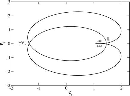
Figure 14: Nyquist curve for $y>y_{max}$ and $\eta>\eta_{c}^{(\pm)}$ (specifically $y=2$ and $\eta=6$). The DF has two maxima at $V_{0}=\pm V_{*}$ and one minimum at $V_{0}=0$. The DF is unstable (with respect to this perturbation) because the Nyquist curve encircles the origin. Since it rotates twice around the origin, this implies that there are $N=2$ unstable modes $(\omega_{r},\omega_{i})$ with $\omega_{i}>0$. Case (- + -).

For $1<y<y_{max}$, there exists two wavenumbers $\eta_{c}^{(0)}(y)$ and $\eta_{c}^{(\pm)}(y)$ at which the DF is marginally stable. The DF has two maxima at $V_{0}=\pm V_{*}$ and one minimum at $V_{0}=0$. For $\eta=\eta_{c}^{(0)}(y)$, the marginal perturbation does not propagate ($\Omega_{r}=0$). For $\eta=\eta_{c}^{(\pm)}(y)$, the marginal perturbation has a pulsation $\Omega_{r}=\pm V_{*}/\sqrt{\eta_{c}}$. By considering the Nyquist curves in this region (see Fig. 15), we find that the DF is stable for $\eta<\eta_{c}^{(\pm)}(y)$ and unstable for $\eta>\eta_{c}^{(\pm)}(y)$.

Figure 15: Nyquist curve for $1<y<y_{max}$ and $\eta>\eta_{c}^{(0)}$ (specifically $y=1.2$ and $\eta=6$). The DF has two maxima at $V_{0}=\pm V_{*}$ and one minimum at $V_{0}=0$. The DF is unstable (with respect to this perturbation) because the Nyquist curve encircles the origin. Since it rotates only once around the origin, this implies that there is $N=1$ unstable mode $(\omega_{r},\omega_{i})$ with $\omega_{i}>0$. Case (- - -).

A few comments are in order:

1. In Fig. 10, we explicitly see that the system is always unstable with respect to perturbations with sufficiently small $k$ (the case of cold systems $T=0$ is treated in Appendix E). This corroborates the general result given at the end of Sec. 3.5. More precisely, we see that the system is stable for perturbations with $k>(k_{c})_{*}$ (corresponding to the solid line) and unstable for perturbations with $k<(k_{c})_{*}$. Furthermore, we note that this critical wavenumber $(k_{c})_{*}$ corresponds to a marginal perturbation where the phase velocity $\omega/k$ coincides with the maximum of the velocity distribution: for $v_{a}^{2}<T$, this is $v_{0}=0$ and for $v_{a}^{2}>T$, this is $v_{0}=\pm v_{*}$.

2. For $1<y<y_{max}$ and $\eta_{c}^{(\pm)}<\eta<\eta_{c}^{(0)}$, there are two unstable modes since the Nyquist curve encircles the origin twice. One of these two modes is $\omega=i\omega_{i}$ and the other is $\omega=\omega_{r}+i\omega_{i}$ with $\omega_{r}\neq 0$ (overstable). When we increase $\eta$ and cross the marginal line $\eta=\eta_{c}^{(0)}$, the mode $\omega=i\omega_{i}$ becomes stable according to the general result (93). Indeed, for $y>1$, the DF is minimum at $v=0$. This is why there is only one unstable mode for $\eta>\eta_{c}^{(0)}$: the mode $\omega=\omega_{r}+i\omega_{i}$ with $\omega_{r}\neq 0$ (overstable). On the other hand, for $y<1$, the mode $\omega=i\omega_{i}$ is stable for $\eta<\eta_{c}^{(0)}$. When we increase $\eta$ and cross the marginal line $\eta=\eta_{c}^{(0)}$, it becomes unstable according to the general result (93). Indeed, for $y>1$, the DF is maximum at $v=0$.

3. In Fig. 10, we see that the critical Jeans length $(\lambda_{c})_{*}$ associated to a double-humped DF ($v_{a}\neq 0$) is always larger than the critical Jeans length associated to the single-humped Maxwellian ($v_{a}=0$). This means that the presence of streaming in a purely stellar system has a stabilizing role. This is different if there exists a gas component in the system since the critical Jeans length is reduced by the relative motion of the gas and stars (Sweet 1963).

4. For a double-humped stellar system with $v_{a}<\sqrt{T}$, the critical Jeans length increases with $v_{a}$ due to the stabilization effect of the relative velocity. Alternatively, in a contra-streaming self-gravitating gas with $v_{a}<c_{s}$, the critical Jeans length decreases with $v_{a}$ and tends to zero as $v_{a}\rightarrow c_{s}$ (Talwar & Kalra 1966, Ikeuchi et al. 1974). On the other hand, for a double-humped stellar system with $v_{a}>\sqrt{T}$ or for a contrastreaming self-gravitating gas with $v_{a}>c_{s}$, the critical Jeans length decreases with $v_{a}$ (but remains larger than the classical Jeans wavelength corresponding to $v_{a}=0$) and overstable modes appear.

7 The asymmetric double-humped distribution

7.1 Determination of the extrema

We now assume that the reduced distribution (51) is an asymmetric double-humped distribution of the form

$$f(v)=\sqrt{\frac{\beta}{2\pi}}\frac{\rho}{1+\Delta}\left[e^{-\frac{\beta}{2}(v-v_{a})^{2}}+\Delta e^{-\frac{\beta}{2}(v+v_{a})^{2}}\right],$$ (205)

where $T=1/\beta$ is the temperature of the Maxwellians and $\Delta$ is the asymmetry parameter (we assume here that $\Delta>1$). This distribution is plotted in Fig. 16. The symmetric case is recovered for $\Delta=1$. The average velocity is $\langle v\rangle=-[(\Delta-1)/(\Delta+1)]v_{a}$ and the kinetic temperature $T_{kin}\equiv\langle(v-\langle v\rangle)^{2}\rangle=T+[4\Delta/(\Delta+1)^{2}]v_{a}^{2}$. The velocities $v_{0}$ at which the distribution function $f(v)$ is extremum satisfy $f^{\prime}(v_{0})=0$. They are determined by the equation

$$e^{-2\beta v_{a}v_{0}}=\frac{1}{\Delta}\frac{v_{a}-v_{0}}{v_{a}+v_{0}}.$$ (206)

We note that $v_{0}\in]-v_{a},+v_{a}[$. Introducing the dimensionless velocity and the dimensionless separation (186), Eq. (206) can be rewritten

$$1=\frac{1}{2V_{a}V_{0}}\ln\left(\frac{V_{a}+V_{0}}{V_{a}-V_{0}}\right)+\frac{\ln(\Delta)}{2V_{a}V_{0}}.$$ (207)

It is convenient to introduce the variables

$$x=\frac{V_{0}}{V_{a}},\qquad y=V_{a}^{2}.$$ (208)

Then, we have to study the function

$$y(x)=\frac{1}{2x}\ln\left(\frac{1+x}{1-x}\right)+\frac{\ln(\Delta)}{2x},$$ (209)

for $x\in]-1,+1[$. This function is plotted in Fig. 17. It has the following properties

$$y(x)\sim-\frac{1}{2}\ln(1-x),\qquad(x\rightarrow 1^{-}),$$ (210)

$$y(x)\sim-\frac{1}{2}\ln(1+x),\qquad(x\rightarrow-1^{+}),$$ (211)

$$y(x)\sim\frac{\ln(\Delta)}{2x},\qquad(x\rightarrow 0).$$ (212)

Considering the negative velocities $x<0$, we note that $y\geq 0$ iff $x\leq x_{0}$ with

$$x_{0}=\frac{1-\Delta}{1+\Delta}.$$ (213)

Considering the positive velocities $x>0$, we note that the curve $y(x)$ is minimum at $x=x_{*}$ where $x_{*}$ is solution of

$$\frac{2x_{*}}{1-x_{*}^{2}}-\ln\left(\frac{1+x_{*}}{1-x_{*}}\right)=\ln(\Delta).$$ (214)

This function is represented in Fig. 18. We note that Eq. (214) has a unique solution $x_{*}$ for each value of $\Delta>1$. Therefore, the function $y(x)$ has a single minimum at $x=x_{*}$. The value of this minimum is

$$y_{*}=\frac{1}{1-x_{*}^{2}}>1.$$ (215)

The extrema of the distribution $f(V)$ can be determined from the study of the function (209). If $y<y_{*}$, the distribution $f(V)$ has a single maximum at $V_{0}=V_{-}<0$. If $y>y_{*}$, the distribution $f(V)$ has two maxima at $V_{0}=V_{-}<0$ and $V_{0}=V_{+}>0$ and one minimum at $V_{0}=V_{p}>0$. These different values are given by $V_{0}=V_{a}y^{-1}(V_{a}^{2})$.

Figure 16: Asymmetric double-humped distribution made of two Mawellians with separation $y$ and asymmetry $\Delta>1$. If $y>y_{*}$, the DF has one global maximum at $V_{0}=V_{-}<0$, a minimum at $V_{0}=V_{p}>0$ and a local maximum at $V_{0}=V_{+}>0$. If $y<y_{*}$, the DF has only one maximum at $V_{0}=V_{-}<0$.

Figure 17: The function $y(x)$ for the asymmetric double-humped distribution.

Figure 18: Evolution of $x_{*}$, $y_{*}$, $x_{c}$ and $y_{c}$ as a function of $\Delta$. The curves intersect each other at $\Delta_{*}=3.3105$.

In conclusion, for a given asymmetry $\Delta>1$ and temperature $T$:

$\bullet$ if $y>y_{*}$, the distribution function $f(V)$ has a global maximum at $V_{0}=V_{-}<0$, a local maximum at $V_{0}=V_{+}>0$ and one minimum at $V_{0}=V_{p}>0$.

$\bullet$ if $y<y_{*}$, the distribution function $f(V)$ has only one maximum at $V_{0}=V_{-}<0$.

7.2 The condition of marginal stability

The dielectric function associated to the asymmetric double-humped distribution is

$$\epsilon(\Omega)=1-\frac{\eta}{1+\Delta}\left[W(\sqrt{\eta}\Omega-\sqrt{y}))+\Delta W(\sqrt{\eta}\Omega+\sqrt{y}))\right],$$

where $W(z)$ is defined in Eq. (106). When $\Omega_{i}=0$, the real and imaginary parts of the dielectric function $\epsilon(\eta,\Omega_{r})=\epsilon_{r}(\eta,\Omega_{r})+i\epsilon_{i}(\eta,\Omega_{r})$ can be written

$$\epsilon_{r}(\eta,\Omega_{r})=1-\frac{\eta}{1+\Delta}[W_{r}(\sqrt{\eta}\Omega_{r}-\sqrt{y}))$$

$$+\Delta W_{r}(\sqrt{\eta}\Omega_{r}+\sqrt{y}))],$$ (217)

$$\epsilon_{i}(\eta,\Omega_{r})=-\frac{\eta}{1+\Delta}[W_{i}(\sqrt{\eta}\Omega_{r}-\sqrt{y}))$$

$$+\Delta W_{i}(\sqrt{\eta}\Omega_{r}+\sqrt{y}))],$$ (218)

where $W_{r}(z)$ and $W_{i}(z)$ are defined in Eqs. (128)-(129) where $z$ is here a real number. The condition of marginal stability corresponds to $\epsilon_{r}(\eta,\Omega_{r})=\epsilon_{i}(\eta,\Omega_{r})=0$. The condition $\epsilon_{i}(\eta,\Omega_{r})=0$ is equivalent to

$$f^{\prime}(\sqrt{\eta}\Omega_{r})=0.$$ (219)

The condition $\epsilon_{r}(\eta,\Omega_{r})=0$ leads to

$$1-\frac{\eta}{1+\Delta}\left[W_{r}(\sqrt{\eta}\Omega_{r}-\sqrt{y}))+\Delta W_{r}(\sqrt{\eta}\Omega_{r}+\sqrt{y}))\right]=0.$$

According to Eq. (219), the phase velocity $\sqrt{\eta}\Omega_{r}$ is equal to a velocity $V_{0}$ at which the distribution (205) is extremum. The second equation (7.2) determines the value(s) $\eta_{c}(y)$ of the wavenumber at which the distribution is marginally stable. Therefore, we have to solve

$$1-\frac{\eta}{1+\Delta}\left[W_{r}(V_{0}-\sqrt{y}))+\Delta W_{r}(V_{0}+\sqrt{y}))\right]=0,$$

where $V_{0}$ is given by

$$1=\frac{1}{2\sqrt{y}V_{0}}\ln\left(\frac{\sqrt{y}+V_{0}}{\sqrt{y}-V_{0}}\right)+\frac{\ln(\Delta)}{2\sqrt{y}V_{0}}.$$ (222)

Eliminating $V_{0}$ between these two expressions yields the critical wavenumber(s) $\eta_{c}(y)$ as a function of $y$. However, it is easier to proceed differently. Setting $x=V_{0}/\sqrt{y}$, we obtain the equations

$$y=\frac{1}{2x}\ln\left(\frac{1+x}{1-x}\right)+\frac{\ln(\Delta)}{2x},$$ (223)

$$\eta=\frac{1+\Delta}{\left[W_{r}(\sqrt{y}(x-1))+\Delta W_{r}(\sqrt{y}(x+1))\right]}.$$ (224)

For given $x$, we can obtain $y$ from Eq. (223) [see also Fig. 17] and $\eta$ from Eq. (224). Varying $x$ in the interval $]-1,1[$ yields the full curve $\eta_{c}(y)$. We have three types of solutions. For $x\in]-1,x_{0}]$, we obtain a branch $\eta_{c}^{(-)}(y)$ where the pulsation of the marginal mode is negative: $\Omega_{r}=V_{-}/\sqrt{\eta_{c}}<0$ corresponding to the global maximum of $f(v)$. For $x\in]0,x_{*}]$, we obtain a branch $\eta_{c}^{(p)}(y)$ where the pulsation of the marginal mode is positive: $\Omega_{r}=V_{p}/\sqrt{\eta_{c}}>0$ corresponding to the minimum of $f(v)$. For $x\in[x_{*},1[$, we obtain a branch $\eta_{c}^{(+)}(y)$ where the pulsation of the marginal mode is positive: $\Omega_{r}=V_{+}/\sqrt{\eta_{c}}>0$ corresponding to the local maximum of $f(v)$. This leads to the curves reported in Figs. 19 and 20 for two values of the asymmetry factor $\Delta$.

For $x\rightarrow-1$, $y\rightarrow+\infty$ and

$$\eta_{c}^{(-)}(y)=\frac{1+\Delta}{\Delta}+\frac{1+\Delta}{4\Delta^{2}y}+...\qquad(y\rightarrow+\infty).$$ (225)

For $x\rightarrow x_{0}$, $y\rightarrow 0$ and

$$\eta_{c}^{(-)}(y)\rightarrow 1\qquad(y\rightarrow 0).$$ (226)

This returns the critical wavenumber (130) associated with the Maxwellian distribution (102) corresponding to $y=0$. For $x\rightarrow 1$, $y\rightarrow+\infty$ and

$$\eta_{c}^{(+)}(y)\sim 1+\Delta+\frac{\Delta(1+\Delta)}{4y}+...\qquad(y\rightarrow+\infty).$$ (227)

Let $x_{c}$ and $y_{c}$ be determined by the equations

$$y_{c}=\frac{1}{2x_{c}}\ln\left(\frac{1+x_{c}}{1-x_{c}}\right)+\frac{\ln(\Delta)}{2x_{c}},$$ (228)

$$W_{r}(\sqrt{y_{c}}(x_{c}-1))+\Delta W_{r}(\sqrt{y_{c}}(x_{c}+1))=0.$$ (229)

For $x\rightarrow x_{c}$, $y\rightarrow y_{c}$ and

$$\eta_{c}^{(s)}(y)\propto\frac{1}{y-y_{c}}\rightarrow+\infty\qquad(y\rightarrow y_{c}),$$ (230)

where $s=p$ if $\Delta<\Delta_{*}$ and $s=+$ if $\Delta>\Delta_{*}$ as will become clear below. Note that there is no physical solution to Eqs. (223)-(224) when $0<x<x_{c}$ ($\eta$ would be negative) so that the branch $\eta_{c}^{(s)}(y)$ starts at $(y_{c},+\infty)$ corresponding to $x=x_{c}$. The evolution of $x_{c}$ and $y_{c}$ with $\Delta$ is studied in Fig. 18 and is compared to the evolution of $x_{*}$ and $y_{*}$. The curves intersect each other at $\Delta_{*}=3.3105$. For $\Delta<\Delta_{*}$, $x_{c}<x_{*}$ so that the stability diagram displays three marginal branches $\eta_{c}^{(-)}(y)$, $\eta_{c}^{(p)}(y)$ and $\eta_{c}^{(+)}(y)$ (see Fig. 19). The branches $\eta_{c}^{(p)}(y)$ and $\eta_{c}^{(+)}(y)$ connect each other at $(y_{*},\eta_{*})$ corresponding to $x=x_{*}$. At that point they touch the line $y=y_{*}$ separating distributions with one or two maxima. For $\Delta=\Delta_{*}$, $x_{c}=x_{*}$ so that the branch $\eta_{c}^{(p)}(y)$ is rejected to infinity and only the branches $\eta_{c}^{(-)}(y)$ and $\eta_{c}^{(+)}(y)$ remain. For $\Delta>\Delta_{*}$, $x_{c}>x_{*}$ so that the phase diagram displays only two marginal branches $\eta_{c}^{(-)}(y)$ and $\eta_{c}^{(+)}(y)$ (see Fig. 20).

7.3 The stability diagram

The critical wavenumbers $\eta_{c}(y)$ corresponding to marginal stability determined previously are represented as a function of the separation $y$ in Figs. 19 and 20 for two values of the asymmetry factor $\Delta$. We recall that $\eta_{c}^{(-)}(y)$ corresponds to the wavenumber associated with a marginal mode with pulsation $\Omega_{r}=V_{-}/\sqrt{\eta_{c}}<0$ (global maximum of $f$), $\eta_{c}^{(p)}(y)$ corresponds to the wavenumber associated with a marginal mode with pulsation $\Omega_{r}=V_{p}/\sqrt{\eta_{c}}>0$ (minimum of $f$) and $\eta_{c}^{(+)}(y)$ corresponds to the wavenumber associated with a marginal mode with pulsation $\Omega_{r}=V_{+}/\sqrt{\eta_{c}}>0$ (local maximum of $f$). We have also plotted the line $y=y_{*}$. On the left of this line, the DF has a single maximum at $V_{-}<0$ and on the right of this line, the DF has two maxima at $V_{-}<0$ and $V_{+}>0$ and a minimum at $V_{p}>0$. In order to investigate the stability of the solutions in the different regions of the parameter space, we have used the Nyquist criterion. The description of the stability diagram is similar to the one given in Sec. 6.3 and the different possible cases can be understood directly from the reading of Figs. 19 and 20. The best way is to fix $y$ and progressively increase the value of $\eta$. For $y<y_{*}$, the distribution has only one maximum at $V_{0}=V_{-}$ so the Nyquist curve has one intersection with the $x$-axis (in addition to the limit point $(1,0)$). For $\eta\rightarrow 0$, we find that $\epsilon_{r}(V_{-})>0$ so the system is stable. As we increase $\eta$ and pass above the solid line, we find that $\epsilon_{r}(V_{-})<0$ so the system is unstable. For $y>y_{*}$, the distribution has two maxima at $V_{0}=V_{-}$ and $V_{0}=V_{+}$ and one minimum at $V_{0}=V_{p}$. At each intersection with a marginal line, one of the values $\epsilon_{r}(V_{-})$, $\epsilon_{r}(V_{p})$ or $\epsilon_{r}(V_{+})$ changes sign. We have indicated by symbols like $(-++)$ the respective signs of $\epsilon_{r}(V_{-})$, $\epsilon_{r}(V_{p})$ and $\epsilon_{r}(V_{+})$. We can then easily draw by hands the corresponding Nyquist curve. Therefore, it is not necessary to show all the possibilities and we have only indicated a few representative cases in Figs. 21-24 for illustration.

Figure 19: Stability diagram of the asymmetric double-humped distribution for $\Delta<\Delta_{*}$ (specifically $\Delta=1.02$). There exists three marginal branches $\eta_{c}^{(-)}(y)$, $\eta_{c}^{(p)}(y)$ and $\eta_{c}^{(+)}(y)$. The symbols have been defined in the text.

Figure 20: Stability diagram of the asymmetric double-humped distribution for $\Delta>\Delta_{*}$ (specifically $\Delta=10$). There exists two marginal branches $\eta_{c}^{(-)}(y)$ and $\eta_{c}^{(+)}(y)$.

Figure 21: $\Delta<\Delta_{*}$: Nyquist curve for $y_{*}<y<y_{c}$ and $\eta<\eta_{c}^{(-)}$ (specifically $\Delta=1.02$, $y=1.1$ and $\eta=1$). The DF has a global maximum at $V_{-}$, a minimum at $V_{p}$ and a local maximum at $V_{+}$. The DF is stable (with respect to this perturbation) because the Nyquist curve does not encircle the origin. Case (+ + +).

Figure 22: $\Delta<\Delta_{*}$: Nyquist curve for $y_{*}<y<y_{c}$ and $\eta_{c}^{(-)}<\eta<\eta_{c}^{(+)}$ (specifically $\Delta=1.02$, $y=1.1$ and $\eta=3.436$). The DF has a global maximum at $V_{-}$, a minimum at $V_{p}$ and a local maximum at $V_{+}$. The DF is unstable (with respect to this perturbation) because the Nyquist curve encircles the origin once. There is $N=1$ unstable mode. Case (- + +).

Figure 23: $\Delta<\Delta_{*}$: Nyquist curve for $y_{*}<y<y_{c}$ and $\eta_{c}^{(+)}<\eta<\eta_{c}^{(p)}$ (specifically $\Delta=1.02$, $y=1.1$ and $\eta=4$). The DF has a global maximum at $V_{-}$, a minimum at $V_{p}$ and a local maximum at $V_{+}$. The DF is unstable (with respect to this perturbation) because the Nyquist curve encircles the origin twice. There are $N=2$ unstable modes. Case (- + -).

Figure 24: $\Delta<\Delta_{*}$: Nyquist curve for $y_{*}<y<y_{c}$ and $\eta>\eta_{c}^{(p)}$ (specifically $\Delta=1.02$, $y=1.1$ and $\eta=6$). The DF has a global maximum at $V_{-}$, a minimum at $V_{p}$ and a local maximum at $V_{+}$. The DF is unstable (with respect to this perturbation) because the Nyquist curve encircles the origin once. There is $N=1$ unstable mode. Case (- - -).

Remark: In Figs. 19 and 20, we see that the system is stable for perturbations with $k>(k_{c})_{*}$ (corresponding to the solid line) and unstable for perturbations with $k<(k_{c})_{*}$. This critical wavenumber $(k_{c})_{*}$ corresponds to a marginal perturbation where the phase velocity $\omega/k$ coincides with the global maximum $v_{0}=v_{-}$ of the velocity distribution.

8 The case of plasmas

We shall now compare the previous results obtained for self-gravitating systems to the case of plasmas.

8.1 A brief historic

The name plasma was introduced by Tonks & Langmuir (1929) to describe an ionised gas made of electrons and ions. They found that cold plasmas oscillate with a natural pulsation $\omega_{p}=(4\pi\rho e^{2}/m^{2})^{1/2}$. In order to take into account thermal effects, plasmas were initially described in terms of hydrodynamic equations. A dispersion relation was derived by Thomson & Thomson (1933) for isothermal perturbations and by Gross (1951) for three dimensional adiabatic perturbations. However, fluid equations do not provide a good description of plasmas and rely on arbitrary assumptions concerning the perturbations (see van Kampen 1957). Indeed, plasmas are essentially collisionless so that a hydrodynamic description is not clearly justified. Vlasov (1938,1945) was the first to attempt to derive the dispersion relation directly from the collisionless Boltzmann equation (nowdays called the Vlasov equation). He obtained the expression of the pulsation $\omega(k)$ in the high wavelength limit. However, Landau (1946) criticized his mathematical treatment showing that there are serious divergences in the integrals considered by Vlasov. Landau performed a rigorous mathematical study using an appropriate contour of integration in the complex plane and showed that the plasma undergoes damped oscillations. The pulsation is in agreement with the expression given by Vlasov but, in addition, the plasma undergoes collisionless damping (nowdays called Landau damping). Following Landau’s seminal work, several authors studied the stability of a plasma. They showed that single-humped distributions are always stable (Berz 1956, Appendix by W. Newcomb in Bernstein 1958, Auer 1958, Penrose 1960, Noerdlinger 1960, Jackson 1960). Then, they considered double humped distributions modeling two contrastreaming beams (Haeff 1949, Nergaard 1948, Pierce & Hebenstreit 1949) and determined particular conditions under which such distributions are unstable (Twiss 1952, Buneman 1958, Auer 1958, Kahn 1959, Buneman 1959, Penrose 1960, Noerdlinger 1960, Jackson 1960). They found qualitatively that the plasma becomes unstable when the stream velocity becomes sensibly larger than the thermal velocity.

After briefly recalling some classical results, we will provide a detailed study of the stability/instability of a double-humped distribution made of two Maxwellians. We shall complete the study of a symmetric double-humped distribution (by explicitly computing the range of unstable wavelengths) and consider for the first time the case of asymmetric double-humped distributions. We will show that the nature of the problem changes above a critical asymmetry $\Delta_{*}=3.3105$.

8.2 The Euler-Poisson system

We consider a plasma made of electrons with mass $m$ and charge $-e$ and ions with mass $m_{i}$ and charge $+e$. We assume the ions to be infinitely massive so that they do not contribute to the motion and only provide a neutralizing background. The fluid equations describing the motion of the electrons can be written

$${\partial\rho\over\partial t}+\nabla\cdot(\rho{\bf u})=0,$$ (231)

$${\partial{\bf u}\over\partial t}+({\bf u}\cdot\nabla){\bf u}=-{1\over\rho}\nabla p-\nabla\Phi,$$ (232)

$$\Delta\Phi=-\frac{4\pi e^{2}}{m^{2}}(\rho-\rho_{i}).$$ (233)

These equations differ from the Euler-Poisson system (1)-(3) describing a self-gravitating barotropic gas only in the sign of the interaction and in the presence of a neutralizing background. This neutralizing background avoids the Jeans swindle since an infinite homogeneous distribution of electrons ($\rho={\rm cst}$, ${\bf u}={\bf 0}$, $\Phi=0$) is a steady state of the fluid equations (231)-(233) provided that the condition of electroneutrality $\rho=\rho_{i}$ is satisfied.

Linearizing the Euler-Poisson system around an infinite homogeneous distribution of electrons and decomposing the perturbations in normal modes of the form $e^{i({\bf k}\cdot{\bf r}-\omega t)}$, we obtain the dispersion relation (Nicholson 1992):

$$\omega^{2}=c_{s}^{2}k^{2}+\omega_{p}^{2},$$ (234)

where $c_{s}^{2}=p^{\prime}(\rho)$ is the velocity of sound and

$$\omega_{p}^{2}\equiv\frac{4\pi\rho e^{2}}{m^{2}},$$ (235)

is the plasma pulsation. For an isothermal equation of state $p=\rho T$, we get

$$\omega^{2}=Tk^{2}+\omega_{p}^{2},$$ (236)

and for a polytropic equation of state $p=K\rho^{\gamma}$, we obtain

$$\omega^{2}=\gamma Tk^{2}+\omega_{p}^{2}.$$ (237)

The dispersion relation (234) shows that a plasma described by fluid equations is always stable. For $k=0$, the pulsation tends to a constant

$$\omega=\pm\omega_{p}.$$ (238)

Therefore, in this limit of small wavenumbers, plasma oscillations do not propagate in space: $\rho({\bf r},t)=\rho({\bf r},0)e^{-i\omega_{p}t}$. This behavior is in marked contrast with all usual types of oscillating phenomena such as acoustic waves for which $\omega=ck$. For large wavenumbers, the dispersion relation approaches that of sound waves: $\omega=\pm c_{s}k$.

Remark: Since $\int\delta\rho\delta\Phi\,d{\bf r}=\frac{m^{2}}{4\pi e^{2}}\int(\Delta\delta\Phi)^{2}\,d{\bf r}>0$ for a plasma, the second variations (12) of the energy functional (10) are always positive: $\delta^{2}{\cal W}>0$. Therefore, the energy functional has a unique (global) minimum and the plasma is nonlinearly dynamically stable with respect to the barotropic Euler-Poisson system.

8.3 The Vlasov-Poisson system

The fluid equations are not very appropriate to describe a plasma because most plasmas are in a regime where the collisions between charges are negligible. Therefore, from now on, we shall describe Coulombian plasmas by the Vlasov-Poisson system

$${\partial f\over\partial t}+{\bf v}\cdot{\partial f\over\partial{\bf r}}-\nabla\Phi\cdot{\partial f\over\partial{\bf v}}=0,$$ (239)

$$\Delta\Phi=-\frac{4\pi e^{2}}{m^{2}}(\rho-\rho_{i}),$$ (240)

which ignores collisions between charges. These equations are similar to the Vlasov-Poisson system (33)-(34) describing collisionless stellar systems except that the sign of the interaction is reversed and that there is a neutralizing background. We shall investigate the linear dynamical stability of an infinite homogeneous medium. Therefore, we consider stationary solutions of the Vlasov equation of the form $f=f({\bf v})$. The dispersion relation can be written (Nicholson 1992):

$$\epsilon(k,\omega)\equiv 1-{4\pi e^{2}\over m^{2}k^{2}}\int_{C}{{f^{\prime}(v)}\over v-\frac{\omega}{k}}dv=0.$$ (241)

As in Sec. 3.3, we have taken ${\bf k}$ along the $z$-axis and noted $v$ for $v_{z}$ and $f(v)$ for $\int f({\bf v})\,dv_{x}dv_{y}$.

In general, the dispersion relation (241) cannot be solved explicitly to obtain $\omega(k)$ except in some very simple cases. For example, for cold systems described by the distribution function $f=\rho\delta({v}-{v}_{0})$, we obtain after an integration by parts

$$\omega=v_{0}k\pm\omega_{p}.$$ (242)

In particular, when $v_{0}=0$, we get

$$\omega=\pm\omega_{p}.$$ (243)

The system is stable to all wavenumbers. We also note that the dispersion relation (243) coincides with the dispersion relation (234) obtained with fluid equations with $c_{s}=0$.

Let us briefly recall important properties of the dispersion relation (241) obtained in plasma physics (Balescu 1963, Nicholson 1992). We consider a symmetric distribution and write the complex pulsation in the form $\omega=\omega_{r}+i\omega_{i}$. When $\omega_{i}\ll\omega_{r}$ (weakly damped perturbations), the complex pulsation is given by

$$\omega_{r}^{2}=\omega_{p}^{2}+3Tk^{2},\qquad\omega_{i}=\frac{\pi\omega_{p}^{3}}{2\rho k^{2}}f^{\prime}\left(\frac{\omega_{p}}{k}\right),$$ (244)

with $T=\langle v^{2}\rangle$ (where we recall that $v=v_{z}$ in the present case). These relations are valid for $k/k_{D}\ll 1$. The real part of the pulsation satisfies a dispersion relation of the form (307) with $c_{s}^{2}=3T$. Therefore, large wavelengths perturbations in a collisionless plasma correspond to one dimensional isentropic perturbations with index $\gamma=3$ in a gas (see Appendix B). This relation dispersion is called the Langmuir wave dispersion relation (Nicholson 1992). On the other hand, when $f^{\prime}(\omega_{p}/k)<0$, the expression of the imaginary part of the pulsation corresponds to Landau damping. If $f^{\prime}(v)\leq 0$ for all $v\geq 0$, as for the Maxwellian, the plasma is stable. For the Maxwell distribution, we get the Landau formula

$$\omega_{i}=-\sqrt{\frac{\pi}{8}}\omega_{p}\left(\frac{k_{D}}{k}\right)^{3}e^{-\frac{k_{D}^{2}}{2k^{2}}},$$ (245)

for the damping rate, where we have introduced the Debye wavenumber

$$k_{D}^{2}\equiv\frac{4\pi e^{2}\beta\rho}{m^{2}}=\beta\omega_{p}^{2},$$ (246)

where $\beta=1/T$ is the inverse temperature. Alternatively, if there exists wavenumbers $k$ such that $f^{\prime}(\omega_{p}/k)>0$, the perturbation grows and the plasma is unstable. Since the expression (244) is valid for small $k$, this implies that $f^{\prime}(v)$ must be positive for large velocities. This corresponds for example to the “bump-on-tail” situation analyzed in plasma physics (Nicholson 1992). The dispersion relation (244)-a was first obtained by Vlasov (1938,1945). However, the derivation given by Vlasov was not rigorous since he evaluated the integral (241) on the real axis on which there is a singularity. Landau (1946) performed a rigorous mathematical study and showed that, in addition to the oscillations, the waves must be damped exponentially leading to equation (244)-b for the damping rate. It is interesting to note that the Langmuir wave dispersion relation (244)-a is rather independent on the precise form of the distribution function (it depends only on the variance $T=\langle v^{2}\rangle$) while the Landau damping (244)-b is very sensitive to the distribution function. For example, the expression of Landau damping for polytropic distributions is given by (see Appendix E of Chavanis & Delfini 2009):

$$\omega_{i}=-\sqrt{\frac{\pi}{8}}B_{n}\omega_{p}\left(\frac{k_{D}}{k}\right)^{3}\left(n-\frac{1}{2}\right)\frac{1}{n+1}$$

$$\times\left[1-\frac{k_{D}^{2}}{2(n+1)k^{2}}\right]_{+}^{n-3/2}.$$ (247)

When $\omega_{r}\ll\omega_{i}$ (heavily damped perturbations), the pulsation is given for the Maxwellian distribution by

$$\omega_{r}=\pm m\frac{\pi\omega_{p}}{2k_{D}}\frac{k}{\sqrt{\ln k}},\qquad\omega_{i}=-\frac{2\omega_{p}}{k_{D}}k\sqrt{\ln k}.$$ (248)

These expressions are valid for $k/k_{D}\rightarrow+\infty$. There exists several branches of solutions parameterized by the odd integer $m$ (but the branch $m=1$ is the most relevant). Expression (248) of the complex pulsation was first obtained by Landau (1946). The evolution of $\omega_{r}(k)$ and $\omega_{i}(k)$ with $k$ for a Maxwellian distribution are represented in Fig. 3 of Jackson (1960) and it can be compared with Fig. 2 for stellar systems. For small $k$, the damping is weak but it increases rapidly for increasing wavenumbers so that the waves are never observed at sufficiently large wavenumbers.

Remark: Let us consider a plasma with a DF of the form $f=f(v^{2})$ with $f^{\prime}<0$. Since $\int\delta\rho\delta\Phi\,d{\bf r}>0$ for a plasma, the second variations (37) of the constrained pseudo entropy (35) are always negative: $\delta^{2}{S}\leq 0$. Therefore, the pseudo entropy has a unique (global) maximum at fixed mass and energy and the plasma is nonlinearly dynamically stable. These variational technics were introduced in the plasma literature by W. Newcomb in Bernstein (1958) and Gardner (1963); see also the review of Holm et al. (1985).

8.4 The condition of marginal stability

When $\omega_{i}=0$, the real and imaginary parts of the dielectric function $\epsilon(k,\omega_{r})=\epsilon_{r}(k,\omega_{r})+i\epsilon_{i}(k,\omega_{r})$ are

$$\epsilon_{r}(k,\omega_{r})=1-{4\pi e^{2}\over m^{2}k^{2}}{P}\int_{-\infty}^{+\infty}{{f^{\prime}(v)}\over v-\frac{\omega_{r}}{k}}dv,$$ (249)

$$\epsilon_{i}(k,\omega_{r})=-{4\pi^{2}e^{2}\over m^{2}k^{2}}f^{\prime}(\omega_{r}/k).$$ (250)

The condition of marginal stability corresponds to $\epsilon(k,\omega)=0$ and $\omega_{i}=0$, i.e. $\epsilon_{r}({k},\omega_{r})=\epsilon_{i}({k},\omega_{r})=0$. We obtain therefore the equations

$$1-\frac{4\pi e^{2}}{m^{2}k^{2}}P\int_{-\infty}^{+\infty}{f^{\prime}(v)\over{v}-{\omega_{r}}/{k}}d{v}=0,$$ (251)

$$f^{\prime}\left({\omega_{r}}/{k}\right)=0.$$ (252)

The second condition (252) imposes that the phase velocity $\omega_{r}/k=v_{ext}$ is equal to a velocity where $f(v)$ is extremum ($f^{\prime}(v_{ext})=0$). The first condition (251) then determines the wavenumber(s) corresponding to marginal stability. It can be written

$$k_{c}=\left(\frac{4\pi e^{2}}{m^{2}}\int_{-\infty}^{+\infty}\frac{f^{\prime}(v)}{v-v_{ext}}\,dv\right)^{1/2}.$$ (253)

Finally, the pulsation(s) corresponding to marginal stability are $\omega_{r}=v_{ext}k_{c}$ and the perturbation behaves like $\delta f\sim e^{-i\omega_{r}t}$.

8.5 Particular solutions of $\epsilon(k,\omega)=0$

We can look for a solution of the dispersion relation $\epsilon(k,\omega)=0$ in the form $\omega=i\omega_{i}$ corresponding to $\omega_{r}=0$. In that case, the perturbation grows ($\omega_{i}>0$) or decays ($\omega_{i}<0$) without oscillating. Like in Sec. 3.8, we shall assume that $f(v)$ is an even function. For $\omega_{i}>0$, the growth rate is given by

$$1-{4\pi e^{2}\over m^{2}k^{2}}\int_{-\infty}^{+\infty}\frac{vf^{\prime}(v)}{v^{2}+\frac{\omega_{i}^{2}}{k^{2}}}\,dv=0.$$ (254)

For $\omega_{i}<0$, the decay rate is given by

$$1-{4\pi e^{2}\over m^{2}k^{2}}\int_{-\infty}^{+\infty}\frac{vf^{\prime}(v)}{v^{2}+\frac{\omega_{i}^{2}}{k^{2}}}\,dv-i\frac{8\pi^{2}e^{2}}{m^{2}k^{2}}f^{\prime}\left(\frac{i\omega_{i}}{k}\right)=0.$$ (255)

Let us assume that the distribution satisfies

$$\int_{-\infty}^{+\infty}\frac{f^{\prime}(v)}{v}\,dv>0.$$ (256)

This is not the generic case. For example, the Maxwell distribution does not satisfy this inequality. If inequality (256) is satisfied, then the marginal mode $\omega=0$ corresponds to the critical wavenumber

$$k_{c}=\left({4\pi e^{2}\over m^{2}}\int_{-\infty}^{+\infty}\frac{f^{\prime}(v)}{v}\,dv\right)^{1/2}.$$ (257)

Furthermore, repeating the steps of Sec. 3.8, we obtain for $k\rightarrow k_{c}$ that

$$\omega_{i}=\frac{k_{c}^{3}m^{2}}{4\pi^{2}e^{2}f^{\prime\prime}(0)}\left(1-\frac{k^{2}}{k_{c}^{2}}\right),\qquad(k\rightarrow k_{c}).$$ (258)

This formula leads to the following result. If the distribution is maximum at $v=0$, so that $f^{\prime\prime}(0)<0$, we find that the mode $\omega=i\omega_{i}$ is stable for $k<k_{c}$ and unstable for $k>k_{c}$. Alternatively, if the distribution is minimum at $v=0$, so that $f^{\prime\prime}(0)>0$, we find that the mode $\omega=i\omega_{i}$ is stable for $k>k_{c}$ and unstable for $k<k_{c}$. This result will be illustrated in connection to Fig. 26 for the symmetric double humped distribution. Note that this result implies that a symmetric distribution satisfying inequality (256) is always unstable (to some wavenumbers).

8.6 The Nyquist method

To apply the Nyquist method, we have to plot the curve $(\epsilon_{r}(k,\omega_{r}),\epsilon_{i}(k,\omega_{r}))$ parameterized by $\omega_{r}$ going from $-\infty$ to $+\infty$ (for a fixed wavenumber $k$). Let us consider the asymptotic behavior for $\omega_{r}\rightarrow\pm\infty$. Since $f(v)$ is positive and tends to zero for $v\rightarrow\pm\infty$, we conclude that $\epsilon_{i}(k,\omega_{r})\rightarrow 0$ for $\omega_{r}\rightarrow\pm\infty$ and that $\epsilon_{i}(k,\omega_{r})<0$ for $\omega_{r}\rightarrow-\infty$ while $\epsilon_{i}(k,\omega_{r})>0$ for $\omega_{r}\rightarrow+\infty$. On the other hand, for $\omega_{r}\rightarrow\pm\infty$, we obtain at leading order

$$\epsilon_{r}(k,\omega_{r})\simeq 1-{4\pi^{2}e^{2}\rho\over m^{2}\omega_{r}^{2}},\qquad(\omega_{r}\rightarrow\pm\infty).$$ (259)

From these results, we conclude that the behavior of the curve close to the point $(1,0)$ is like the one represented in Fig. 25. For $\omega_{r}/k=v_{ext}$, where $v_{ext}$ is a velocity at which the distribution is extremum $(f^{\prime}(v_{ext})=0)$, the imaginary part of the dielectric function $\epsilon_{i}(k,kv_{ext})=0$ and the real part of the dielectric function

$$\epsilon_{r}(k,kv_{ext})=1-{4\pi^{2}e^{2}\over m^{2}k^{2}}\int_{-\infty}^{\infty}\frac{f^{\prime}(v)}{v-v_{ext}}\,dv.$$ (260)

Subtracting the value $f^{\prime}(v_{ext})=0$ in the numerator of the integrand, and integrating by parts, we obtain

$$\epsilon_{r}(k,kv_{ext})=1+{4\pi^{2}e^{2}\over m^{2}k^{2}}\int_{-\infty}^{+\infty}\frac{f(v_{ext})-f(v)}{(v-v_{ext})^{2}}\,dv.$$ (261)

If $v_{Max}$ denotes the velocity corresponding to the global maximum of the distribution, we clearly have

$$\epsilon_{r}(k,kv_{Max})>1.$$ (262)

8.6.1 Single-humped distributions

Let us assume that the distribution $f(v)$ has a single maximum at $v=v_{0}$ (so that $f^{\prime}(v_{0})=0$) and tends to zero for $v\rightarrow\pm\infty$. Then, the Nyquist curve cuts the $x$-axis ($\epsilon_{i}(k,\omega_{r})$ vanishes) at the limit point $(1,0)$ when $\omega_{r}\rightarrow\pm\infty$ and at the point $(\epsilon_{r}(k,kv_{0}),0)$ when $\omega_{r}/k=v_{0}$. Due to its behavior close to the limit point $(1,0)$, the fact that it rotates in the counterclockwise sense, and the property that $\epsilon_{r}(k,kv_{0})>1$ according to Eq. (262), the Nyquist curve must necessarily behave like in Fig. 25. Therefore, the Nyquist curve starts on the real axis at $\epsilon_{r}(k,\omega_{r})=1$ for $\omega_{r}\rightarrow-\infty$, then going in counterclockwise sense it crosses the real axis at the point $\epsilon_{r}(k,kv_{0})>1$ and returns on the real axis at $\epsilon_{r}(k,\omega_{r})=1$ for $\omega_{r}\rightarrow+\infty$. Therefore, it cannot encircle the origin. According to the Nyquist criterion exposed in Sec. 3.5, we conclude that a single-humped distribution is always linearly dynamically stable.

Figure 25: Nyquist curve for the Maxwell distribution. The DF is always stable.

Let us specifically consider the Maxwell distribution (102) for illustration. The dielectric function (241) associated to the Maxwell distribution is

$$\epsilon(k,\omega)=1+\frac{4\pi e^{2}}{m^{2}k^{2}}\left(\frac{\beta}{2\pi}\right)^{1/2}\rho\int_{C}\frac{\beta v}{v-\frac{\omega}{k}}e^{-\beta{v^{2}\over 2}}\ dv.$$ (263)

Introducing the Debye wavenumber (246), it can be rewritten

$$\epsilon({k},\omega)=1+{k_{D}^{2}\over k^{2}}W\biggl{(}{\sqrt{\beta}\omega\over k}\biggr{)}.$$ (264)

It will be convenient in the following to work with dimensionless quantities. We introduce the dimensionless wavenumber and the dimensionless pulsation

$$\eta=\frac{k_{D}^{2}}{k^{2}},\qquad\Omega=\frac{\omega}{\omega_{p}}.$$ (265)

Noting that $\sqrt{\beta}\omega/k=\sqrt{\eta}\Omega$, the dielectric function (264) can be rewritten

$$\epsilon({\eta},\Omega)=1+\eta W(\sqrt{\eta}\Omega).$$ (266)

When $\Omega_{i}=0$, the real and imaginary parts of the dielectric function $\epsilon(\eta,\Omega_{r})=\epsilon_{r}(\eta,\Omega_{r})+i\epsilon_{i}(\eta,\Omega_{r})$ are given by

$$\epsilon_{r}(\eta,\Omega_{r})=1+\eta W_{r}\left(\sqrt{\eta}\Omega_{r}\right),$$ (267)

$$\epsilon_{i}(\eta,\Omega_{r})=\eta W_{i}\left(\sqrt{\eta}\Omega_{r}\right).$$ (268)

The Nyquist curve for the Maxwell distribution is represented in Fig. 25.

On the other hand, if we consider a polytrope of index $n=1/2$ (waterbag distribution) as in Sec. 5.5, we find that the dielectric function is given by

$$\epsilon(k,\omega)=1+\frac{k_{D}^{2}}{3k^{2}}W_{1/2}\left(\frac{\omega}{k\sqrt{T}}\right),$$ (269)

where $W_{1/2}(x)$ is given by Eq. (175). The condition $\epsilon(k,\omega)=0$ determines the dispersion relation. We get

$$\omega^{2}=\omega_{p}^{2}+3Tk^{2}.$$ (270)

We note that, for the water-bag distribution, the general asymptotic behavior (244) becomes exact. We also note that for the specific index $n=1/2$ ($\gamma=3$), the dispersion relation in a collisionless stellar system takes the same form as in a gas (see Sec. 8.2).

8.6.2 Double-humped distributions

Let us consider a double-humped distribution with a global maximum at $v_{Max}$, a minimum at $v_{min}$ and a local maximum at $v_{max}$. We assume $v_{Max}<v_{min}<v_{max}$. The Nyquist curves starts at $(1,0)$, progresses in the counterclockwise sense and crosses the $x$-axis at $\epsilon_{r}(v_{Max})>1$, then at $\epsilon_{r}(v_{min})$ and $\epsilon_{r}(v_{max})$. We can convince ourselves by making drawings of the following results. If

$(+++)$: $\epsilon_{r}(v_{Max})>0$, $\epsilon_{r}(v_{min})>0$, $\epsilon_{r}(v_{max})>0$,

$(+--)$: $\epsilon_{r}(v_{Max})>0$, $\epsilon_{r}(v_{min})<0$, $\epsilon_{r}(v_{max})<0$,

$(++-)$: $\epsilon_{r}(v_{Max})>0$, $\epsilon_{r}(v_{min})>0$, $\epsilon_{r}(v_{max})<0$,

the Nyquist curve does not encircle the origin so the system is stable. If

$(+-+)$: $\epsilon_{r}(v_{Max})>0$, $\epsilon_{r}(v_{min})<0$, $\epsilon_{r}(v_{max})>0$,

the Nyquist curve rotates one time around the origin so that there is one mode of instability. Since $\epsilon_{r}(v_{Max})>0$ there is no mode of marginal stability with $\omega_{r}/k=v_{Max}$. Cases $(+++)$, $(+-+)$ and $(+--)$ are observed in Sec. 8.8 for an asymmetric double-humped distribution made of two Maxwellians.

If the double-humped distribution is symmetric with respect to the origin with two maxima at $\pm v_{*}$ and a minimum at $v=0$, we get the same results as above with the additional properties $\epsilon_{r}(v_{Max})=\epsilon_{r}(v_{max})=\epsilon_{r}(v_{*})>1$ and $\epsilon_{r}(v_{min})=\epsilon_{r}(0)$. We have only two cases $(+++)$ and $(+-+)$. They are observed in Sec. 8.7 for a symmetric double-humped distribution made of two Maxwellians. Since $\epsilon_{r}(v_{*})>0$, there is no mode of marginal stability with $\omega_{r}/k=\pm v_{*}$.

It can be shown that a plasma is unstable (to some wavelengths) iff $f(v)$ has a minimum at a value $v=v_{min}$ such that

$$\int_{-\infty}^{+\infty}{{f^{\prime}(v)}\over v-v_{min}}dv=\int_{-\infty}^{+\infty}\frac{f(v)-f(v_{min})}{(v-v_{min})^{2}}\,dv>0.$$ (271)

This result was proven by Penrose (1960) and it is sometimes called the Penrose criterion. This criterion can be deduced from the Nyquist method as follows. A double-humped distribution $f(v)$ is unstable if there exists a range of $k$ such that we are in the situation $(+-+)$, i.e. $\epsilon_{r}(v_{min})<0$ and $\epsilon_{r}(v_{max})>0$. The first condition can be satisfied (for sufficiently small $k$) iff condition (271) is realized, which is the Penrose criterion. Then, the range of unstable wavenumbers is

$$\frac{4\pi e^{2}}{m^{2}}\int_{-\infty}^{+\infty}{{f^{\prime}(v)}\over v-v_{max}}dv<k^{2}<\frac{4\pi e^{2}}{m^{2}}\int_{-\infty}^{+\infty}{{f^{\prime}(v)}\over v-v_{min}}dv.$$

(272)

If the first integral is negative, the range of unstable wavenumbers is $k<k_{c}^{(min)}$. This corresponds to Fig. 31 and to the region $y>y_{c}$ in Fig. 32. If the first integral is positive, the range of unstable wavenumbers is $k_{c}^{(max)}<k<k_{c}^{(min)}$. This corresponds to the region $y_{*}<y<y_{c}$ in Fig. 32 (indeed, $y_{c}$ corresponds precisely to the case where the first integral becomes equal to zero).

8.7 The symmetric double-humped distribution

Let us now consider the symmetric double-humped distribution (184). In the plasma case, the dielectric function can be written

$$\epsilon(\eta,\Omega)=1+\frac{\eta}{2}\left[W(\sqrt{\eta}\Omega-\sqrt{y}))+W(\sqrt{\eta}\Omega+\sqrt{y}))\right],$$

where $\eta$ (wavelength) and $\Omega$ (pulsation) are defined by Eq. (265) and $y$ (separation) is defined by Eq. (188). The condition of marginal stability corresponds to $\epsilon(k,\omega)=0$ and $\omega_{i}=0$. The condition $\epsilon_{i}(k,\omega_{r})=0$ is equivalent to $f^{\prime}(\omega_{r}/k)=0$ so that the phase velocity $\omega_{r}/k=v_{0}$ corresponds to the velocities where the distribution is extremum. Then, the wavenumbers at which the distribution is marginally stable are obtained by solving $\epsilon_{r}(k,\omega_{r}=kv_{0})=0$. Proceeding as in Sec. 6 and introducing the parameter $x=V_{0}/V_{a}$, we find that the equations determining the critical wavenumbers $\eta_{c}(y)$ are given by

$$y=\frac{1}{2x}\ln\left(\frac{1+x}{1-x}\right),$$ (274)

$$\eta=\frac{-2}{\left[W_{r}(\sqrt{y}(x-1))+W_{r}(\sqrt{y}(x+1))\right]}.$$ (275)

We note that only the sign in Eq. (275) changes with respect to the study of the gravitational case, so we can readily adapt the results of Sec. 6 to the present situation by simply reverting the sign. For $\sqrt{\eta}\Omega_{r}=\pm V_{*}$, corresponding to $x\neq 0$, there is no physical solution to Eqs. (274)-(275) with positive $\eta>0$. Therefore, in the plasma case, there is no marginal mode with non zero pulsation for the symmetric double-humped distribution (in agreement with the general discussion of Sec. 8.6.2). We now consider the marginal mode with $\Omega_{r}=0$. This corresponds to the “degenerate” solution $x=0$ (for any $y$) for which Eqs. (274)-(275) reduce to

$$\eta_{c}^{(0)}(y)=\frac{-1}{W_{r}(\sqrt{y})}.$$ (276)

According to Fig. 9, physical solutions exist only for $y\geq y_{max}=z_{c}^{2}=1.708$. We note that the range of parameters that was forbidden in the gravitational case is now allowed in the plasma case and vice versa. For $y<y_{max}$, the system is stable. This result is to be expected since, for $y=0$, the distribution (184) reduces to the Maxwellian that is stable for a repulsive interaction. We now consider the range $y\in[y_{max},+\infty[$. For $y\rightarrow y_{max}$, we have

$$\eta_{c}^{(0)}(y)\sim\frac{2y_{max}}{y-y_{max}},\qquad(y\rightarrow y_{max}).$$ (277)

On the other hand, the curve $\eta_{c}^{(0)}(y)$ has a minimum at $(4.511,3.512)$ (see Appendix A of Chavanis & Delfini 2009). Finally, for $y\rightarrow+\infty$, we have

$$\eta_{c}^{(0)}(y)\sim y\rightarrow+\infty,\qquad(y\rightarrow+\infty).$$ (278)

Again this result is expected because, for $y\rightarrow+\infty$, the two humps do not “see” each other and behave as two independent single-humps distributions that are stable in the repulsive case.

The critical wavenumber $\eta_{c}^{(0)}(y)$ corresponding to marginal stability determined previously is represented as a function of the separation $y$ in Fig. 26. We have also plotted the line $y=1$. On the left of this line, the distribution has a single maximum at $V_{0}=0$ and on the right, the distribution has two maxima at $V_{0}=\pm V_{*}$ and a minimum at $V_{0}=0$. In order to investigate the stability of the solutions in the different regions, we have used the Nyquist criterion.

Figure 26: Stability diagram of the symmetric double-humped distribution (184) in the case of plasmas.

For $y<1$, the DF has only one maximum at $V_{0}=0$. There is no marginal mode and the distribution is always stable (see Fig. 27).

Figure 27: Nyquist curve for $y<1$ (specifically $y=0.5$ and $\eta=6$). The DF is stable for any perturbation. Case (+).

For $1<y<y_{max}$, the DF has a minimum at $V_{0}=0$ and two maxima at $\pm V_{*}$. There is no marginal mode and the distribution is always stable (see Figs. 28).

Figure 28: Nyquist curve for $1<y<y_{max}$ (specifically $y=1.2$ and $\eta=6$). The DF is stable for any perturbation. Case (+ + +).

For $y>y_{max}$, the distribution has a minimum at $V_{0}=0$ and two maxima at $\pm V_{*}$. There exists one wavenumber $\eta_{c}^{(0)}$ at which the distribution is marginally stable. For $\eta=\eta_{c}^{(0)}$, the marginal perturbation does not propagate ($\Omega_{r}=0$). By considering the Nyquist curves in this region (see Figs. 29-30), we find that the DF is stable for $\eta<\eta_{c}^{(0)}$ and unstable for $\eta>\eta_{c}^{(0)}$.

Figure 29: Nyquist curve for $y>y_{max}$ and $\eta<\eta_{c}^{(0)}$ (specifically $y=5$ and $\eta=2$). The DF is stable for this range of wavenumbers. Case (+ + +).

Figure 30: Nyquist curve for $y>y_{max}$ and $\eta>\eta_{c}^{(0)}$ (specifically $y=5$ and $\eta=6$). There is one mode of instability in this range of wavenumbers. Case (- + -).

Let us make some remarks:

1. If we consider all possible perturbations, Fig. 26 shows that a symmetric double-humped distribution is stable if $y<y_{max}$ (i.e. $v_{a}<1.307\,T^{1/2}$) and unstable if $y>y_{max}$ (i.e. $v_{a}>1.307\,T^{1/2}$). Therefore, instability occurs when the drift velocity $v_{a}$ is sensibly larger than the thermal speed $\sqrt{T}$ so that the two humps are well separated. In particular, at $T=0$, a double-humped distribution is always unstable to some wavelengths (see Appendix E). More precisely, a symmetric double-humped distribution with $y>y_{max}$ is stable for perturbations with wavenumbers $k>(k_{c})_{*}$ (corresponding to the solid line) and unstable for perturbations with wavenumbers $k<(k_{c})_{*}$. The critical wavenumber $(k_{c})_{*}$ corresponds to the marginal perturbation for which the phase velocity $\omega/k$ coincides with the minimum of the velocity distribution: $v_{0}=0$.

2. For $y>y_{max}$, the mode $\omega=i\omega_{i}$ is stable for $\eta<\eta_{c}^{(0)}$ and it becomes unstable when we increase $\eta$ above the marginal line $\eta=\eta_{c}^{(0)}$. This is consistent with the general result (258) since, for $y>1$, the DF is minimum at $v_{0}=0$.

3. For a double-humped distribution, the critical wavelength is infinite for $v_{a}\leq\sqrt{y_{max}T}$ (stable), then decreases, reaches a minimum and increases again. By contrast, if the plasma is modeled as a contrastreaming gas, the critical wavelength is infinite for $v_{a}<c_{s}$ (stable), then jumps discontinuously to zero at $v_{a}=c_{s}$ and increases for $v_{a}>c_{s}$ (Ikeuchi et al. 1974).

8.8 The asymmetric double-humped distribution

The dielectric function associated to the asymmetric double-humped distribution (205) in the plasma case is

$$\epsilon(\eta,\Omega)=1+\frac{\eta}{1+\Delta}\biggl{[}W(\sqrt{\eta}\Omega-\sqrt{y}))$$

$$+\Delta W(\sqrt{\eta}\Omega+\sqrt{y}))\biggr{]}.$$ (279)

Proceeding as in Sec. 7 and introducing the parameters $x=V_{0}/V_{a}$ and $y=V_{a}^{2}$, we find that the equations determining the critical wavenumbers $\eta_{c}(y)$ are given by

$$y=\frac{1}{2x}\ln\left(\frac{1+x}{1-x}\right)+\frac{\ln(\Delta)}{2x},$$ (280)

$$\eta=-\frac{1+\Delta}{\left[W_{r}(\sqrt{y}(x-1))+\Delta W_{r}(\sqrt{y}(x+1))\right]}.$$ (281)

Equation (280) determines the extrema of the distribution $f(v)$ and Eq. (281) determines the wavenumbers corresponding to the modes of marginal stability. As in Sec. 7, the curve $\eta_{c}(y)$ can be obtained by varying $x$ between $-1$ and $+1$. In the plasma case, there exists physical solutions with positive $\eta$ only for $0<x\leq x_{c}$. For $x\rightarrow 0^{+}$, using Eq. (280), we find that $y\rightarrow+\infty$. Then, we get

$$\eta_{c}^{(p)}(y)\sim y\rightarrow+\infty,\qquad(y\rightarrow+\infty).$$ (282)

For $x\rightarrow x_{c}$, we find that $y\rightarrow y_{c}$ and

$$\eta_{c}^{(s)}(y)\propto\frac{1}{y-y_{c}}\rightarrow+\infty,\qquad(y\rightarrow y_{c}),$$ (283)

where $s=p$ if $\Delta<\Delta_{*}$ and $s=+$ if $\Delta>\Delta_{*}$. For $\Delta<\Delta_{*}$, we get only one marginal branch $\eta_{c}^{(p)}(y)$ corresponding to the mode $\Omega_{r}=V_{p}/\sqrt{\eta_{c}}>0$ (see Fig. 31). For $\Delta>\Delta_{*}$, we get two marginal branches $\eta_{c}^{(p)}(y)$ and $\eta_{c}^{(+)}(y)$ corresponding to the modes $\Omega_{r}=V_{p}/\sqrt{\eta_{c}}>0$ and $\Omega_{r}=V_{+}/\sqrt{\eta_{c}}>0$ (see Fig. 32). They connect each other at $(y_{*},\eta_{*})$ corresponding to $x=x_{*}$. At that point they touch the line $y=y_{*}$ separating distributions with one or two maxima.

Figure 31: Stability diagram of the asymmetric double-humped distribution for $\Delta<\Delta_{*}$ (specifically $\Delta=1.02$). There exists one marginal branch $\eta_{c}^{(p)}(y)$.

Figure 32: Stability diagram of the asymmetric double-humped distribution for $\Delta>\Delta_{*}$ (specifically $\Delta=50$). There exists two marginal branches $\eta_{c}^{(p)}(y)$ and $\eta_{c}^{(+)}(y)$.

The stability diagrams corresponding to the asymmetric double-humped distribution with $\Delta<\Delta_{*}$ and $\Delta>\Delta_{*}$ are represented in Figs. 31 and 32. To investigate the stability of the solutions in the different regions of the parameter space, we have used the Nyquist criterion. If $\Delta<\Delta_{*}$, the description of the stability diagram can be made in continuity with the case of a symmetric double-humped distribution: for $y<y_{c}$ (i.e. $v_{a}^{2}<y_{c}(\Delta)T$), the plasma is stable to all perturbations; for $y>y_{c}$ (i.e. $v_{a}^{2}>y_{c}(\Delta)T$), the plasma is stable for $k>k_{c}^{(p)}(v_{a})$ and unstable for $k<k_{c}^{(p)}(v_{a})$. If $\Delta>\Delta_{*}$, the stability diagram changes: for $y<y_{*}$ (i.e. $v_{a}^{2}<y_{*}(\Delta)T$), the plasma is stable to all perturbations; for $y_{*}<y<y_{c}$ (i.e. $y_{*}(\Delta)T<v_{a}^{2}<y_{c}(\Delta)T$), the plasma is stable for $k>k_{c}^{(p)}(v_{a})$, unstable for $k_{c}^{(+)}(v_{a})<k<k_{c}^{(p)}(v_{a})$ and stable for $k<k_{c}^{(+)}(v_{a})$: this is similar to a re-entrant phase; for $y>y_{c}$ (i.e. $v_{a}^{2}>y_{c}(\Delta)T$), the plasma is stable for $k>k_{c}^{(p)}(v_{a})$ and unstable for $k<k_{c}^{(p)}(v_{a})$. In conclusion, instability occurs when the drift velocity is sensibly larger than the thermal speed so that the two humps are well separated. However, the precise threshold changes whether the asymmetry is smaller or larger than $\Delta_{*}$. For $\Delta<\Delta_{*}$, the plasma is stable iff $v_{a}^{2}<y_{c}(\Delta)T$ and for $\Delta>\Delta_{*}$, the plasma is stable iff $v_{a}^{2}<y_{*}(\Delta)T$.

Figure 33: $\Delta>\Delta_{*}$: Nyquist curve for $y_{*}<y<y_{c}$ and $\eta<\eta_{c}^{(p)}$ (specifically $\Delta=50$, $y=5$ and $\eta=5$). The DF has a global maximum at $V_{-}$, a minimum at $V_{p}$ and a local maximum at $V_{+}$. The DF is stable (with respect to this perturbation) because the Nyquist curve does not encircle the origin. Case (+ + +).

Figure 34: $\Delta>\Delta_{*}$: Nyquist curve for $y_{*}<y<y_{c}$ and $\eta_{c}^{(p)}<\eta<\eta_{c}^{(+)}$ (specifically $\Delta=50$, $y=5$ and $\eta=15$). The DF has a global maximum at $V_{-}$, a minimum at $V_{p}$ and a local maximum at $V_{+}$. The DF is unstable (with respect to this perturbation) because the Nyquist curve encircles the origin once. There is $N=1$ unstable mode. Case (+ - +).

Figure 35: $\Delta>\Delta_{*}$: Nyquist curve for $y_{*}<y<y_{c}$ and $\eta>\eta_{c}^{(+)}$ (specifically $\Delta=50$, $y=5$ and $\eta=30$). The DF has a global maximum at $V_{-}$, a minimum at $V_{p}$ and a local maximum at $V_{+}$. The DF is stable (with respect to this perturbation) because the Nyquist curve does not encircle the origin. Case (+ - -).

9 Conclusion

We have carried out an exhaustive study of the linear dynamical stability/instability of an infinite and homogeneous self-gravitating medium with respect to perturbations with wavenumber $k$. This is the classical Jeans problem that describes the growth of perturbations and the emergence of structures (like stars and galaxies) in astrophysics and cosmology. We have considered the case of a collision-dominated gas described by the Euler equation or the case of a collisionless stellar system described by the Vlasov equation. In the latter case, we have studied single-humped distributions as well as symmetric and asymmetric double-humped distributions. We have used the Nyquist theorem to settle the stability of the system. Detailed stability diagrams in the $(v_{a},k)$ plane for different values of the asymmetry parameter $\Delta$ have been obtained. We have also derived general analytical results concerning the dispersion relation. Finally, we have studied the case of Coulombian plasmas in parallel. The general methods developed here to study the stability of a homogeneous self-gravitating medium can have applications in other domains, not necessarily astrophysics, where the system is described by the Euler or the Vlasov equations coupled to a mean field equation for the potential. One example is the HMF model (Chavanis & Delfini 2009). Although the structure of the problem is the same, the results and the stability diagrams differ because the potential of interaction is different. Many generalizations of our work are possible, changing the potential of interaction or the class of distribution functions, but the present paper provides many methods and analytical results that can be useful to investigate more general situations.

Appendix A Equivalence between the variational problems $(\ref{vh4})$ and $(\ref{ep10})$

The equivalence between the variational problems $(\ref{vh4})$ and $(\ref{ep10})$ has been discussed in previous works (Chavanis 2006a,2008b). We shall here provide a new derivation of this result. To that purpose, we shall show the equivalence between the stability conditions (12) and (39).

First of all, using the identities $f^{\prime}(\epsilon)=-\beta/C^{\prime\prime}(f)$ (see Sec. 3.1) and $p^{\prime}(\rho)=-\rho/\rho^{\prime}(\Phi)$ (see Sec. 2.1), we can rewrite the second variations (39) and (12) in the form

$$\delta^{2}F=-\frac{1}{2}\int\frac{(\delta f)^{2}}{f^{\prime}(\epsilon)}\,d{\bf r}d{\bf v}+\frac{1}{2}\int\delta\rho\delta\Phi\,d{\bf r},$$ (284)

$$\delta^{2}{\cal W}=-\frac{1}{2}\int\frac{(\delta\rho)^{2}}{\rho^{\prime}(\Phi)}\,d{\bf r}+\frac{1}{2}\int\delta\rho\delta\Phi\,d{\bf r}.$$ (285)

We shall determine the perturbation $\delta f_{*}({\bf r},{\bf v})$ that minimizes $\delta^{2}F[\delta f]$ given by Eq. (284) with the constraint $\delta\rho=\int\delta f\,d{\bf v}$. Since the specification of $\delta\rho$ determines $\delta\Phi$, hence the second integral in Eq. (284), we can write the variational problem in the form

$$\delta\left(-\frac{1}{2}\int\frac{(\delta f)^{2}}{f^{\prime}(\epsilon)}\,d{\bf r}d{\bf v}\right)-\int\lambda({\bf r})\delta\left(\int\delta f\,d{\bf v}\right)\,d{\bf r}=0,$$

where $\lambda({\bf r})$ is a Lagrange multiplier. This gives

$$\delta f_{*}=-\lambda({\bf r})f^{\prime}(\epsilon),$$ (287)

and it is a global minimum of $\delta^{2}F[\delta f]$ with the previous constraint since $\delta^{2}(\delta^{2}F)=-\frac{1}{2}\int\frac{\delta(\delta f)^{2}}{f^{\prime}(\epsilon)}\,d{\bf r}d{\bf v}\geq 0$ (the constraint is linear in $\delta f$ so its second variations vanish). The Lagrange multiplier is determined from the constraint $\delta\rho=\int\delta f\,d{\bf v}$ yielding $\delta\rho=-\lambda\int f^{\prime}(\epsilon)\,d{\bf v}$. Therefore, the optimal perturbation (287) can be finally written

$$\delta f_{*}=\frac{\delta\rho}{\int f^{\prime}(\epsilon)\,d{\bf v}}f^{\prime}(\epsilon).$$ (288)

Therefore, $\delta^{2}F[\delta f]\geq\delta^{2}F[\delta f_{*}]$. Explicating $\delta^{2}F[\delta f_{*}]$ using Eqs. (284) and (288), we obtain

$$\delta^{2}F[\delta f]\geq-\frac{1}{2}\int\frac{(\delta\rho)^{2}}{\int f^{\prime}(\epsilon)\,d{\bf v}}\,d{\bf r}+\frac{1}{2}\int\delta\rho\delta\Phi\,d{\bf r}.$$ (289)

Finally, using $\rho^{\prime}(\Phi)=\int f^{\prime}(\epsilon)\,d{\bf v}$, the foregoing inequality can be rewritten

$$\delta^{2}F[\delta f]\geq-\frac{1}{2}\int\frac{(\delta\rho)^{2}}{\rho^{\prime}(\Phi)}\,d{\bf r}+\frac{1}{2}\int\delta\rho\delta\Phi\,d{\bf r}\equiv\delta^{2}{\cal W}[\delta\rho],$$

where the r.h.s. is precisely the functional (285). Furthermore, there is equality in Eq. (A) iff $\delta f=\delta f_{*}$. This proves that the stability criteria (12) and (39) are equivalent. Indeed: (i) if inequality (12) is fulfilled for all perturbations $\delta\rho$ that conserve mass, then according to Eq. (A), we know that inequality (39) is fulfilled for all perturbations $\delta f$ that conserve mass. (ii) if there exists a perturbation $\delta\rho_{*}$ that makes $\delta^{2}{\cal W}[\delta\rho]<0$, then the perturbation $\delta f_{*}$ given by Eq. (288) with $\delta\rho=\delta\rho_{*}$ makes $\delta^{2}F[\delta f]=\delta^{2}{\cal W}[\delta\rho]<0$. In conclusion, the stability criteria (12) and (39) are equivalent.

Appendix B Fluid equations

In a collisional gas, the evolution of the distribution function $f({\bf r},{\bf v},t)$ is governed by Boltzmann’s transport equation

$${\partial f\over\partial t}+{\bf v}\cdot{\partial f\over\partial{\bf r}}-\nabla\Phi\cdot{\partial f\over\partial{\bf v}}=\left({\partial f\over\partial t}\right)_{coll},$$ (291)

where $(\partial f/\partial t)_{coll}$ is the collision operator. This operator locally conserves the mass, the impulse and the kinetic energy. The Boltzmann equation relaxes towards the Maxwellian distribution for $t\rightarrow+\infty$ due to collisions. From Eq. (291), we can easily derive a hierarchy of hydrodynamic equations satisfied by the local moments of the velocity distribution. Defining the density $\rho=\int f\,d{\bf v}$, the local velocity ${\bf u}=\int f{\bf v}\,d{\bf v}$ and the kinetic temperature $\frac{d}{2}\rho T=\frac{1}{2}\int fw^{2}\,d{\bf v}$ (where ${\bf w}={\bf v}-{\bf u}$ is the relative velocity and $d$ the dimension of space), the first three equations of this hierarchy are

$${\partial\rho\over\partial t}+\nabla\cdot(\rho{\bf u})=0,$$ (292)

$${\partial{u_{i}}\over\partial t}+u_{j}\frac{\partial{u}_{i}}{\partial x_{j}}=-{1\over\rho}\frac{\partial P_{ij}}{\partial x_{j}}-\frac{\partial\Phi}{\partial x_{i}},$$ (293)

$$\frac{d}{2}\rho\left(\frac{\partial T}{\partial t}+{\bf u}\cdot\nabla T\right)=-\nabla{\bf q}-P_{ij}\frac{\partial u_{j}}{\partial x_{i}},$$ (294)

where $P_{ij}=\int fw_{i}w_{j}\,d{\bf v}$ is the pressure tensor and ${\bf q}=\frac{1}{2}\int fw^{2}{\bf w}\,d{\bf v}$ is the current of heat. These equations are known as the Maxwell equations of transfer (van Kampen 1957) or as the Jeans equations (Binney & Tremaine 1987). For a collision-dominated gas, we can close this hierarchy of hydrodynamic equations by using a Chapman-Enskog expansion which is valid when the mean free path in the gas is short. The zeroth-order approximation amounts to making the local thermodynamic equilibrium (L.T.E.) assumption

$$f_{L.T.E.}({\bf r},{\bf v},t)=\left(\frac{1}{2\pi T({\bf r},t)}\right)^{d/2}\rho({\bf r},t)e^{-\frac{({\bf v}-{\bf u}({\bf r},t))^{2}}{2T({\bf r},t)}}.$$

This yields ${\bf q}={\bf 0}$ and $P_{ij}=p\delta_{ij}$ where $p=\frac{1}{d}\int fw^{2}\,d{\bf v}=\rho T$ is the pressure. In that case, we obtain the Euler equations (Huang 1966)

$${\partial\rho\over\partial t}+\nabla\cdot(\rho{\bf u})=0,$$ (296)

$${\partial{\bf u}\over\partial t}+{\bf u}\cdot\nabla{\bf u}=-{1\over\rho}\nabla p-\nabla\Phi,$$ (297)

$$\frac{d}{2}\left(\frac{\partial T}{\partial t}+{\bf u}\cdot\nabla T\right)+T\nabla\cdot{\bf u}=0.$$ (298)

$$p=\rho T.$$ (299)

Equation (298) can be rewritten in the form

$$\frac{d}{dt}\left(\frac{\rho}{T^{d/2}}\right)=0,$$ (300)

where $d/dt=\partial/\partial t+{\bf u}\cdot\nabla$ is the material derivative. This equation expresses the conservation of the entropy by the Euler equation (dissipative effects appear at the next order in the Chapman-Enskog expansion leading to the Navier-Stokes equations). We have therefore a closed system of hydrodynamic equations. The steady states correspond to ${\bf u}={\bf 0}$ and to the condition of hydrostatic equilibrium (8). However, at the level of the Euler equations, nothing determines $T({\bf r})$ at equilibrium, i.e. there exists steady states of Eqs. (296)-(299) with any temperature profile $T({\bf r})$. Two cases are particularly relevant. If we consider that the collisions had time to establish a statistical equilibrium state, then $T({\bf r})=T$ is uniform at equilibrium yielding an isothermal equation of state $p({\bf r})=\rho({\bf r})T$. By contrast, if collisions had not time to establish a statistical equilibrium state, we can consider a steady state where the specific entropy is uniform in the whole system: $s({\bf r})=s$. This is equivalent to having $\rho({\bf r})/T({\bf r})^{d/2}$, $p({\bf r})/T({\bf r})^{(d+2)/2}$ or $p({\bf r})/\rho({\bf r})^{(d+2)/d}$ spatially uniform at equilibrium. We then obtain a polytropic equation of state $p({\bf r})=K\rho({\bf r})^{\gamma}$ with

$$\gamma=\frac{c_{p}}{c_{v}}=\frac{d+2}{d}.$$ (301)

In that case, the temperature behaves like $T({\bf r})=K\rho({\bf r})^{\gamma-1}$. The isothermal distribution is justified by taking into account dissipative effects (e.g. using the Navier-Stokes equations) and the polytropic distribution is justified by completely ignoring dissipative effects. However, even if an isothermal distribution has been established under the effect of collisions, when we investigate the dynamical stability of such a distribution, we can usually ignore dissipative effects and use the Euler equations (296)-(299). This is because the dynamical time is in general much shorter than the collisional relaxation time.

If we consider the stability of an infinite homogeneous self-gravitating system or plasma described by the hydrodynamic equations (296)-(299), we find that the dispersion relation is of the form (13) or (234) with

$$c_{s}^{2}=\frac{\delta p}{\delta\rho}.$$ (302)

In the present case, $\delta p/\delta\rho\neq p^{\prime}(\rho)$ since the gas is not barotropic. Linearizing Eq. (300) around the steady state, it reduces to

$$\frac{\partial}{\partial t}\delta\left(\frac{\rho}{T^{d/2}}\right)=0,$$ (303)

so that $\rho/T^{d/2}$, $p/T^{(d+2)/2}$ or $p/\rho^{(d+2)/d}$ are independent on time in the linear regime. Therefore, the perturbations are adiabatic and we have

$$\frac{\delta p}{p}=\frac{d+2}{d}\frac{\delta\rho}{\rho},$$ (304)

yielding $\delta p=\gamma T\delta\rho$ hence

$$c_{s}^{2}=\gamma T.$$ (305)

Regrouping all these results, the dispersion relation for a self-gravitating system or a plasma described by the (non barotropic) Euler equations (296)-(299) are

$$\omega^{2}=\gamma Tk^{2}-4\pi G\rho,$$ (306)

$$\omega^{2}=\gamma Tk^{2}+\omega_{p}^{2}.$$ (307)

The are valid for any equilibrium distribution, e.g. isothermal or polytropic.

Let us now consider the case of a collisionless system described by the Vlasov equation obtained from Eq. (291) by neglecting the collision term. The hydrodynamic equations (292)-(294) remain valid but, in the present case, the L.T.E assumption is not justified anymore so that the hierarchy of equations cannot be closed. However, for $k\rightarrow 0$, the dispersion relation based on the Vlasov equation is given for a self-gravitating system by (see Sec. 3.8):

$$\omega_{i}^{2}=4\pi G\rho-3Tk^{2}-...$$ (308)

This dispersion relation is consistent with Eq. (306) with $\gamma=3$ (corresponding to $d=1$). Therefore, for large wavelengths, a collisionless stellar system can be treated by fluid equations experiencing a one dimensional adiabatic perturbation. For $k\rightarrow 0$, the dispersion relation based on the Vlasov equation are given for a plasma by (see Sec. 8.3):

$$\omega_{r}^{2}=\omega_{p}^{2}+3Tk^{2}+...,\qquad\omega_{i}=\frac{\pi\omega_{p}^{3}}{2\rho k^{2}}f^{\prime}\left(\frac{\omega_{r}}{k}\right).$$ (309)

The Landau damping is due to collective effects and cannot be obtained in a hydrodynamic approximation. However, the dispersion relation for the pulsation $\omega_{r}$ is consistent with Eq. (307) with $\gamma=3$ (corresponding to $d=1$). Therefore, for large wavelengths, the oscillations of a collisionless plasma can be treated by fluid equations experiencing a one dimensional adiabatic compression.

Appendix C Calculation of $I$ for isothermal and polytropic distributions

Let us define

$$I=\int_{-\infty}^{+\infty}\frac{f^{\prime}(v)}{v}\,dv.$$ (310)

For the isothermal distribution (102), the integration is straightforward and yields

$$I_{iso}=-\beta\rho.$$ (311)

For the polytropic distribution (158), the integrals can be expressed in terms of Gamma functions. After simplification, using $\Gamma(x+1)=x\Gamma(x)$, we obtain

$$I_{poly}=-\frac{\beta\rho}{\gamma},$$ (312)

which includes the isothermal distribution (311) as a special case corresponding to $\gamma=1$.

Appendix D Direct calculation of $W(ix)$

Let us compute $W(z)$ defined by Eq. (106) when $z=ix$. When $x>0$, using Eq. (53), we have

$$W(ix)=\frac{1}{\sqrt{2\pi}}\int_{-\infty}^{+\infty}\frac{t}{t-ix}e^{-t^{2}/2}\,dt.$$ (313)

Multiplying the numerator by $t+ix$ and noting that the imaginary part vanishes by symmetry, we obtain

$$W(ix)=\frac{1}{\sqrt{2\pi}}\int_{-\infty}^{+\infty}\frac{t^{2}}{t^{2}+x^{2}}e^{-t^{2}/2}\,dt.$$ (314)

For any real $x$, we have the identity

$$\frac{1}{\sqrt{2\pi}}\int_{-\infty}^{+\infty}\frac{t^{2}}{t^{2}+x^{2}}e^{-t^{2}/2}\,dt=$$

$$1-\sqrt{\frac{\pi}{2}}|x|e^{x^{2}/2}\left[1-{\rm erf}\left(\frac{|x|}{\sqrt{2}}\right)\right].$$ (315)

Therefore, for $x>0$, we obtain

$$W(ix)=1-\sqrt{\frac{\pi}{2}}xe^{x^{2}/2}{\rm erfc}\left(\frac{x}{\sqrt{2}}\right).$$ (316)

When $x<0$, using Eq. (55), we have

$$W(ix)=\frac{1}{\sqrt{2\pi}}\int_{-\infty}^{+\infty}\frac{t}{t-ix}e^{-t^{2}/2}\,dt-\sqrt{2\pi}xe^{x^{2}/2},$$ (317)

which is the same as

$$W(ix)=\frac{1}{\sqrt{2\pi}}\int_{-\infty}^{+\infty}\frac{t^{2}}{t^{2}+x^{2}}e^{-t^{2}/2}\,dt-\sqrt{2\pi}xe^{x^{2}/2}.$$ (318)

Using identity (315) and the fact that ${\rm erf}(-x)=-{\rm erf}(x)$, we finally obtain for $x<0$:

$$W(ix)=1-\sqrt{\frac{\pi}{2}}xe^{x^{2}/2}{\rm erfc}\left(\frac{x}{\sqrt{2}}\right).$$ (319)

Comparing Eqs. (316) and (319), and noting that $W(0)=1$, we see that such expressions are valid for any real $x$.

Appendix E The case of two cold streams

We consider a distribution function of the form

$$f(v)=\frac{\rho}{2}\left(\delta(v+v_{a})+\delta(v-v_{a})\right),$$ (320)

corresponding to two symmetric cold streams ($T=0$) moving in opposite direction with velocity $\pm v_{a}$. We shall consider the stability of this distribution with respect to the Vlasov equation for self-gravitating systems, plasmas and for the HMF model.

Self-gravitating systems: integrating by parts, the dispersion relation (52) can be rewritten

$$1+\frac{4\pi G}{k^{2}}\int\frac{f(v)}{\left(v-\frac{\omega}{k}\right)^{2}}\,dv=0.$$ (321)

For the distribution (320), we obtain

$$k^{2}=-2\pi G\rho\left[\frac{1}{\left(v_{a}+\frac{\omega}{k}\right)^{2}}+\frac{1}{\left(v_{a}-\frac{\omega}{k}\right)^{2}}\right].$$ (322)

This is a $4$th degree equation for $\omega$ with real coefficients. Therefore, it admits $4$ complex solutions that occur in pairs which are complex conjugate of one another, i.e. $\omega_{1,2}=\omega_{r}\pm i\omega_{i}$ and $\omega_{3,4}=\omega^{\prime}_{r}\pm i\omega^{\prime}_{i}$. Accordingly, the system is stable for a perturbation of wavenumber $k$ iff the four roots are real ($\omega_{i}=\omega^{\prime}_{i}=0$). However, it is clear that Eq. (322) has no solution with real $\omega$ so that the distribution (320) is always unstable (to any wavenumber). In fact, the roots of this equation can be obtained analytically. They are given by

$$\omega^{2}=v_{a}^{2}k^{2}-2\pi G\rho\left(1\pm\sqrt{1-\frac{2k^{2}v_{a}^{2}}{\pi G\rho}}\right).$$ (323)

Let us introduce the wavenumber

$$k_{0}=\left(\frac{\pi G\rho}{2}\right)^{1/2}\frac{1}{v_{a}}.$$ (324)

If $k<k_{0}$, then $\omega^{2}$ is real negative so that $\omega$ is purely imaginary. In that case, the perturbation grows without oscillating ($\omega_{r}=0$, $\omega_{i}>0$). On the other hand, if $k>k_{0}$, then $\omega^{2}$ and $\omega$ are complex. In that case, the perturbation grows and oscillates ($\omega_{r}\neq 0$, $\omega_{i}>0$). This is called overstability. Therefore, two cold streams are unstable for $k<k_{0}$ and overstable for $k>k_{0}$. If we consider an asymmetric distribution, we find that the system is always overstable.

Plasmas: in the case of plasmas, performing the transformation $G\rightarrow-e^{2}/m^{2}$, the dispersion relation becomes

$$k^{2}=\frac{2\pi e^{2}\rho}{m^{2}}\left[\frac{1}{\left(v_{a}+\frac{\omega}{k}\right)^{2}}+\frac{1}{\left(v_{a}-\frac{\omega}{k}\right)^{2}}\right].$$ (325)

From the graph of the function $k^{2}=F(\omega/k)$, we find that Eq. (325) has $4$ real roots if $k>k_{c}$ where

$$k_{c}=\left(\frac{4\pi e^{2}\rho}{m^{2}}\right)^{1/2}\frac{1}{v_{a}}.$$ (326)

Therefore, the distribution (320) is stable for $k>k_{c}$ and unstable for $k<k_{c}$. The roots of Eq. (325) are given by

$$\omega^{2}=v_{a}^{2}k^{2}+\frac{2\pi e^{2}\rho}{m^{2}}\left(1\pm\sqrt{1+\frac{2k^{2}v_{a}^{2}m^{2}}{\pi e^{2}\rho}}\right).$$ (327)

The solutions with the sign $+$ correspond to $\omega^{2}$ real positive (pure oscillations). The solutions with the sign $-$ correspond to $\omega^{2}$ real positive if $k>k_{c}$ (pure oscillations) and to $\omega^{2}$ real negative if $k<k_{c}$. In that case, $\omega$ is purely imaginary so that the perturbation grows without oscillating ($\omega_{r}=0$, $\omega_{i}>0$). There is no overstable mode. If we consider an asymmetric distribution with asymmetry $\Delta$, we find that $k_{c}^{2}=4\pi e^{2}\rho/m^{2}v_{a}^{2}$ as for the symmetric case. For $k<k_{c}$, the system is overstable.

HMF model: for the attractive HMF model, performing the transformation $k\rightarrow 1$ and $4\pi G\rightarrow k/2$, the dispersion relation becomes

$$1=-\frac{k\rho}{4}\left[\frac{1}{\left(v_{a}+\omega\right)^{2}}+\frac{1}{\left(v_{a}-\omega\right)^{2}}\right],$$ (328)

where $k$ is the coupling constant. The distribution (320) is always unstable. The roots of Eq. (328) are given by

$$\omega^{2}=v_{a}^{2}-\frac{k\rho}{4}\left(1\pm\sqrt{1-\frac{16v_{a}^{2}}{k\rho}}\right).$$ (329)

Let us introduce the velocity

$$v_{0}=\left(\frac{k\rho}{16}\right)^{1/2}.$$ (330)

If $v_{a}<v_{0}$, then $\omega^{2}$ is real negative so that $\omega$ is purely imaginary. In that case, the perturbation increases without oscillating ($\omega_{r}=0$, $\omega_{i}>0$). On the other hand, if $v_{a}>v_{0}$, then $\omega^{2}$ and $\omega$ are complex. In that case, the perturbation increases and oscillates ($\omega_{r}\neq 0$, $\omega_{i}>0$). Therefore, two cold streams are unstable for $v_{a}<v_{0}$ and overstable for $v_{a}>v_{0}$. If we consider an asymmetric distribution, we find that the system is always overstable.

For the repulsive HMF model, performing the transformation $k\rightarrow-k$, the dispersion relation becomes

$$1=\frac{k\rho}{4}\left[\frac{1}{\left(v_{a}+\omega\right)^{2}}+\frac{1}{\left(v_{a}-\omega\right)^{2}}\right].$$ (331)

From the graph of the curve $F(\omega)=1$, we find that Eq. (331) has $4$ real roots if $v_{a}>v_{c}$ where

$$v_{c}=\left(\frac{k\rho}{2}\right)^{1/2}.$$ (332)

Therefore, the distribution (320) is stable for $v_{a}>v_{c}$ and unstable for $v_{a}<v_{c}$. The roots of Eq. (331) are given by

$$\omega^{2}=v_{a}^{2}+\frac{k\rho}{4}\left(1\pm\sqrt{1+\frac{16v_{a}^{2}}{k\rho}}\right).$$ (333)

The solutions with the sign $+$ correspond to $\omega^{2}$ real positive (pure oscillations). The solutions with the sign $-$ correspond to $\omega^{2}$ real positive if $v_{a}>v_{c}$ (pure oscillations) and to $\omega^{2}$ real negative if $v_{a}<v_{c}$. In that case, $\omega$ is purely imaginary so that the perturbation increases without oscillating ($\omega_{r}=0$, $\omega_{i}>0$). There is no overstable mode. If we consider an asymmetric distribution with asymmetry $\Delta$, we find that $v_{c}^{2}=(\Delta+1)k\rho/4$. For $v<v_{c}$, the system is overstable.

References

- (1) Antonov, V.A. 1960a, Astr. Zh, 37, 918 (translated in: Sov. Astron., 4, 859, (1961))
- (2) Antonov, V.A. 1960b, Astr. Zh, 37, 918
- (3) Antonov, V.A. 1962, Vest. Leningr. Gos. Univ., 7, 135
- (4) Arnol’d, V.I. 1966, Izv. Vyssh. Ucheb. Zaved. Matem, 54, 3 (translated in: Am. Math. Soc. Transl. 79, 267 (1969))
- (5) Araki, S. 1987, ApJ, 94, 99
- (6) Auer, P.L. 1958, PRL, 1, 411
- (7) Balescu, R. 1963, Statistical Mechanics of Charged Particles (Interscience, New York)
- (8) Bartholomew, P. 1971, MNRAS, 151, 333
- (9) Bernstein, I. 1958, Phys. Rev., 109, 10
- (10) Berz, F. 1956, Proc. Phys. Soc., 69, 939
- (11) Binney, J., & Tremaine, S. 1987, Galactic Dynamics (Princeton Series in Astrophysics)
- (12) Bohm, D. & Gross, E.P. 1949, Phys. Rev., 75, 1851
- (13) Bouchet, F. & Barré, F. 2005, J. Stat. Phys., 118, 1073
- (14) Buneman, O. 1958, PRL, 1, 8
- (15) Buneman, O. 1959, Phys. Rev., 115, 503
- (16) Campa, A., Chavanis, P.H., Giansanti, A., Morelli, G. 2008, PRE, 78, 040102(R)
- (17) Chandrasekhar, S. 1942 An Introduction to the Theory of Stellar Structure (Dover)
- (18) Chandrasekhar, S. 1961, Hydrodynamic and Hydromagnetic Stability (Oxford University Press).
- (19) Chandrasekhar, S. 1964, ApJ, 139, 664
- (20) Chavanis, P.H. 2002a, A&A, 381, 340
- (21) Chavanis, P.H. 2002b, A&A, 386, 732
- (22) Chavanis, P.H. 2006a, A&A, 451, 109
- (23) Chavanis, P.H. 2006b, EPJB, 52, 433
- (24) Chavanis, P.H. 2008a, EPJB, 62, 179
- (25) Chavanis, P.H. 2008b, AIP Conf. Proc., 970, 39
- (26) Chavanis, P.H., 2009, EPJB, 70, 73
- (27) Chavanis, P.H., Delfini, L. 2009, EPJB, 69, 389
- (28) Chavanis, P.H., Sire, C. 2005, Physica A, 356, 419
- (29) Chavanis, P.H., Vatteville, J., Bouchet, F. 2005, EPJB, 46, 61
- (30) Choi, M.Y. & Choi, J. 2003, PRL, 91, 124101
- (31) Dauxois, T., Ruffo, S., Arimondo, E. & Wilkens, M. 2002, Dynamics and thermodynamics of systems with long range interactions (Lecture Notes in Physics, Springer)
- (32) Doremus, J.P., Feix, M., Baumann, G. 1971, PRL, 26, 725
- (33) Du Jiulin, 2006, Astrophys. Space Sci., 306, 247
- (34) Eddington, A.S. 1918, MNRAS, 79, 2
- (35) Ellis, R., Haven, K. & Turkington, B. 2000 J. Stat. Phys., 101, 999
- (36) Ellis, R., Haven, K. & Turkington, B. 2002 Nonlin., 15, 239
- (37) Gardner, C.S. 1963 Phys. Fluids., 6, 839
- (38) Gross, E.P. 1951 Phys. Rev., 82, 232
- (39) Haeff, A.V. 1949 Proc. Inst. Rad. Engrs., 37, 4
- (40) Harris, E.G. 1959 PRL, 2, 34
- (41) Holm, D.D., Marsden, J.E., Ratiu , T., & Weinstein, A. 1985, Phys. Rep. 123, 1
- (42) Huang, K. 1966, Statistical Mechanics (Wiley)
- (43) Ichimaru, S. 1973, Basic Principles of Plasma Physics (W.A. Benjamin, Inc. Reading, Mass.)
- (44) Ikeuchi, S., Nakamura, T. & Takahara, F. 1974, Prog. Theor. Phys., 52, 1807
- (45) Inagaki, S. & Konishi, T. 1993, Publ. Astron. Soc. Japan, 45, 733
- (46) Ipser, J.R. 1974, ApJ, 193, 463
- (47) Ipser, J.R. & Horwitz, G. 1979, ApJ, 232, 863
- (48) Jackson, J.D. 1960, J. Nucl. Energy., 1, 171
- (49) Jeans, J.H. 1902, Phil. Trans. R. Soc. Lond. A, 199, 1
- (50) Jeans, J.H. 1915, MNRAS, 76, 70
- (51) Jeans, J.H. 1929, Astronomy and Cosmogony (Cambridge University Press)
- (52) Kahn, F.D. 1959, ApJ, 129, 468
- (53) Kandrup, H. 1991, ApJ, 370, 312
- (54) Kandrup, H. & Sygnet, J.F. 1985, ApJ, 298, 27
- (55) Keller, E. & Segel, L.A. 1970, J. Theoret. Biol., 26, 399
- (56) Kronberger, T., Leubner, M. P. & van Kampen, E. 2006, A&A 453, 21
- (57) Landau, L. 1946, Journ. of Phys., 10, 25
- (58) Ledoux, P. 1945, ApJ, 102, 143
- (59) Lemou, M., Méhats, F. & Raphael P. 2009, preprint
- (60) Leubner, M.P. 2005 ApJ, 632, L1
- (61) Liboff, R.L. 1963, Phys. Lett., 3, 322
- (62) Lima, J.A.S. , Silva, R., & Santos, J. 2002 A&A, 396, 309
- (63) Lima, J.A.S., & de Souza, R.E. 2005 Physica A, 350, 303
- (64) Lynden-Bell, D. 1962, MNRAS, 124, 279
- (65) Lynden-Bell, D. 1967, in: Relativity and Astrophysics, Vol. 2: Galactic Structure (Lectures in Applied Mathematics, Vol. 9. Edited by Jürgen Ehlers. Providence, Rhode Island: American Mathematical Society).
- (66) Lynden-Bell, D. & Sanitt, N. 1969, MNRAS, 143, 167
- (67) Lynden-Bell, D., & Wood, R. 1968, MNRAS, 138, 495
- (68) Nergaard, L.S. 1948, RCA Rev., 9, 585
- (69) Nicholson, D.R. 1992, Introduction to Plasma Theory (Krieger Publishing Company, Florida)
- (70) Noerdlinger, P.D. 1959, Phys. Rev., 118, 879
- (71) Nyquist, H. 1932, Bell System Tech. J., 11, 126
- (72) Padmanabhan, T. 1990, Phys. Rep., 188, 285
- (73) Penrose, O. 1960, Phys. Fluids, 3, 258
- (74) Peebles, J. 1980, Large-Scale Structures of the Universe (Princeton University Press)
- (75) Pichon, C. 1994, Ph.D. thesis, Cambridge
- (76) Pierce J.R. & Hebenstreit W.B. 1949, Bell. Syst. Tech. J., 28, 33
- (77) Plastino A.R. & Plastino A. 1993, Phys. Lett. A, 174, 384
- (78) Semelin, B., Sanchez, N. & de Vega, H.J. 2001, PRD, 63, 084005
- (79) Silva, R. & Alcaniz, J.S. 2004, Physica A, 341, 208
- (80) Simon, R. 1961, Acad. Roy. Belg. Bull. Sci., 47, 731
- (81) Summers, D. & Thorne, R.M. 1991, Phys. Fluids B, 3, 1835
- (82) Sweet, P.A. 1963, MNRAS, 125, 285
- (83) Talwar, S.P. & Kalra, G.R. 1966, Ann. Astrophys., 29, 507
- (84) Taruya, A. & Sakagami, M. 2003a, Physica A, 322, 285
- (85) Taruya, A. & Sakagami, M. 2003b, PRL, 90, 181101
- (86) Thomson, J.J. & Thomson, G.P. 1933, Conduction of Electricity through Gases (Cambridge University Press)
- (87) Thorne, R.M. & Summers, D. 1991, Phys. Fluids B, 3, 2117
- (88) Tonks, L. & Langmuir, I. 1929, Phys. Rev., 33, 195
- (89) Toomre, A. 1964, ApJ, 139, 1217
- (90) Tremaine, S., Hénon, M., & Lynden-Bell, D. 1986 MNRAS, 219, 285
- (91) Tsallis, C. 1988, J. Stat. Phys., 52, 479
- (92) Twiss, R.Q. 1952, Phys. Rev., 88, 1392
- (93) van Kampen, N.G. 1957, Physica, 23, 641
- (94) Vlasov, A. 1938, Journ. Exper. a. Theor. Phys., 8, 291
- (95) Vlasov, A. 1945, Journ. of Phys., 9, 25
- (96) Weinberg, M.D. 1991, ApJ, 368, 66
- (97) Yamaguchi, Y., Barré, J., Bouchet, F., Dauxois, T. & Ruffo, S. 2004, Physica A, 337, 36