Orbital magnetoelectric coupling in band insulators

Abstract

Magnetoelectric responses are a fundamental characteristic of materials that break time-reversal and inversion symmetries (notably multiferroics) and, remarkably, of “topological insulators” in which those symmetries are unbroken. Previous work has shown how to compute spin and lattice contributions to the magnetoelectric tensor. Here we solve the problem of orbital contributions by computing the frozen-lattice electronic polarization induced by a magnetic field. One part of this response (the “Chern-Simons term”) can appear even in time-reversal-symmetric materials and has been previously shown to be quantized in topological insulators. In general materials there are additional orbital contributions to all parts of the magnetoelectric tensor; these vanish in topological insulators by symmetry and also vanish in several simplified models without time-reversal and inversion whose magnetoelectric couplings were studied before. We give two derivations of the response formula, one based on a uniform magnetic field and one based on extrapolation of a long-wavelength magnetic field, and discuss some of the consequences of this formula.

I Introduction

Understanding the response of a solid to applied magnetic or electric fields is of both fundamental and applied interest. Two standard examples are that metals can be distinguished from insulators by their screening of an applied electric field, and superconductors from metals by their exclusion of magnetic field (the Meissner effect). Magnetoelectric response in insulators has been studied for many years and is currently undergoing a renaissance driven by the availability of new materials. The linear response of this type is the magnetoelectric polarizability: in “multiferroic” materials that break parity and time-reversal symmetries, an applied electric field creates a magnetic dipole moment and a magnetic field creates an electric dipole moment, and several applications have been proposed for such responses. Such responses are observed in a variety of materials and from a variety of mechanisms.Spaldin and Fiebig (2005); Fiebig (2005) From a theoretical point of view, the most intriguing part of the polarizability is that due to the orbital motion of electrons, because the orbital motion couples to the vector potential rather than the more tangible magnetic field.

The orbital magnetoelectric polarizability has also been studied recently in non-magnetic materials known as “topological insulators.” These insulators have Bloch wavefunctions with unusual topological properties, that lead to a magnetoelectric response described by an ${\mathbf{E}}\cdot{\mathbf{B}}$ term in their effective electromagnetic Lagrangians, Qi et al. (2008) with a quantized coefficient. Qi, Hughes, and Zhang Qi et al. (2008) (QHZ) gave a formula for the coefficient of this term. For the specific case of topological band insulators, their result reproduces earlier formulas for the relevant topological invariant, Fu et al. (2007); Moore and Balents (2007); Roy but it is more generally valid: it describes a contribution to the magnetoelectric polarizability non just in topological insulators but in any band insulator. Their formula has a periodicity or ambiguity by $e^{2}/h$ that is related to the possibility of surface quantum Hall layers on a three-dimensional sample and generalizes the ambiguity of ordinary polarization.

The same ${\mathbf{E}}\cdot{\mathbf{B}}$ coupling, known as “axion electrodynamics” and originally studied in the 1980s, Wilczek (1987) was obtained in a previous paper by three of the present authors Essin et al. (2009) using a semiclassical approach Xiao et al. (2009) to compute $dP/dB$, the polarization response to an applied magnetic field. However, in a general material, that semiclassical approach leads to an explicit formula for only part of the orbital magnetoelectric polarizability, the part found by QHZ. Qi et al. (2008) The remainder, which is generically nonvanishing in materials that break inversion and time-reversal symmetries, is expressed only implicitly in terms of the modification of the Bloch wavefunctions by the magnetic field.

In this paper, we develop a more microscopic approach that enables us to compute all terms in the orbital response explicitly in terms of the unperturbed wavefunctions, thereby opening the door to realistic calculations using modern band-structure methods (e.g., in the context of density-functional theory). Moreover, beyond its importance for computation, this expression clarifies the physical origins of the orbital magnetoelectric polarizability and resolves some issues that arose in previous efforts to describe the “toroidal moment” in periodic systems.

In the remainder of this introduction, we review some macroscopic features of the magnetoelectric response, while subsequent sections will be devoted mainly to a detailed treatment of microscopic features. The magnetoelectric tensor can be decomposed into trace and traceless parts as

$$\frac{\partial P^{i}}{\partial B^{j}}=\frac{\partial M_{j}}{\partial E_{i}}=\alpha^{i}_{j}=\tilde{\alpha}^{i}_{j}+\alpha_{\theta}\delta^{i}_{j},$$ (1)

where $\tilde{\alpha}$ is traceless and

$$\alpha_{\theta}=\frac{\theta}{2\pi}\frac{e^{2}}{h}$$ (2)

is the trace part expressed in terms of the dimensionless parameter $\theta$; $\alpha$ has the physical dimension of conductance. The trace is the most difficult term to determine, as its physical effects are elusive. It should be noted that equality between $\partial P^{i}/\partial B^{j}$ and $\partial M_{j}/\partial E_{i}$ only holds in the absence of dissipation and dispersion, which describes the low frequency, low temperature responses of an insulator. Hehl et al. (2008); Hornreich and Shtrikman (1968) The placement of the indices in Eq. (1) is not essential for the arguments and calculations in this paper, and the reader can choose to treat $\alpha$ as a Cartesian tensor $\alpha_{ij}$ if desired. foo As a Cartesian tensor, the traceless part decomposes further into symmetric and antisymmetric parts

$$\tilde{\alpha}^{S}_{ij}=\frac{1}{2}\left(\tilde{\alpha}_{ij}+\tilde{\alpha}_{ji}\right),\quad\tilde{\alpha}^{A}_{ij}=\frac{1}{2}\left(\tilde{\alpha}_{ij}-\tilde{\alpha}_{ji}\right)=-\epsilon_{ijk}T_{k},$$ (3)

where $T_{i}=-\epsilon_{ijk}\tilde{\alpha}_{jk}/2$ is the toroidal response. (Unless otherwise stated, in our work repeated indices are implicitly summed.) The terminology reflects that this part of the orbital magnetoelectric response is related to the “toroidal moment”, which is an order parameter that has recently been studied intensively; in a Landau effective free energy, the toroidal moment and the toroidal part of the magnetoelectric response are directly related. Ederer and Spaldin (2007); Batista et al. (2008)

The primary goal of this paper is to compute the contribution to $\alpha$ that arises solely from the motion of electrons due to their couplings to the electromagnetic potentials $\rho\phi$ and $-\mathbf{j}\cdot\mathbf{A}$. We call this contribution the orbital magnetoelectric polarizability, or OMP for short. Other effects, such as those mediated by lattice distortions or the Zeeman coupling to the electron’s spin, are calculable with known methods.Wojdeł and Íñiguez (2009) We shall only treat the polarization response to an applied magnetic field here; concurrent work by Malashevich, Souza, Coh, and one of us obtains an equivalent formula by developing methods to compute the orbital magnetization induced by an electrical field.Malashevich et al. (to be published)

The magnetoelectric tensor’s physical consequences arise through the bound current and charge,Qi et al. (2008); Hehl et al. (2008) given by $\rho_{b}=-\mathrm{div}\,\mathbf{P}$ and $\mathbf{J}_{b}=\partial_{t}\mathbf{P}+\mathrm{curl}\,{\mathbf{M}}$. Besides having a ground state value, each moment responds (instantaneously and locally, as appropriate for the low-frequency response of an insulator) to applied electric and magnetic fields, e.g., $P^{i}=P_{0}^{i}+\chi_{E}^{ij}E_{j}+\alpha^{i}_{j}B^{j}$; we will concentrate on the magnetoelectric response. (Unless otherwise stated, in this article repeated indices are implicitly summed.) It is useful to allow $\alpha^{i}_{j}$, a material property, to vary in space and time by allowing the electronic Hamiltonian to vary; this leads to a formula that covers the effects of boundaries and time-dependent shearing of the crystal, for example. Then the relevant terms are

$$J^{i}_{b} =(\tilde{\alpha}^{l}_{j}\epsilon^{ikj}-\tilde{\alpha}^{i}_{j}\epsilon^{jkl})\partial_{k}E_{l} +(\partial_{t}\alpha^{i}_{j})B^{j}+\epsilon^{ijk}(\partial_{j}\alpha^{l}_{k})E_{l}$$

$$\rho_{b} =-\tilde{\alpha}^{i}_{j}\partial_{i}B^{j} -(\partial_{i}\alpha^{i}_{j})B^{j},$$ (4)

We have used two of Maxwell’s equations to simplify the first term in each line. The most important point to notice here is that $\alpha_{\theta}$ does not appear except in derivatives, so that any uniform and static contribution to $\theta$ has no effect on electrodynamics. Hence in a uniform, static crystal, the components of $\tilde{\alpha}$ can be computed or measured from the current or charge response to spatially varying fields, given by the first term in each line. On the other hand, if we wish similarly to obtain $\alpha_{\theta}$ from charge or current responses to applied fields, we need to consider a crystal that varies either spatially or temporally, so that ${\mathbf{E}}$ or ${\mathbf{B}}$ will couple to $\partial_{i}\alpha_{\theta}$ or $\partial_{t}\alpha_{\theta}$, as in the second terms of Eqs. (I). These considerations, which we will elaborate later, motivate our theoretical approach to the OMP in this paper.

We will proceed as follows. In Section II, we present the results of our calculation of the OMP in the independent-electron approximation. This section includes a review of known results, followed by a discussion of the new contributions we compute and when those contributions can be expected to vanish (so that the OMP reduces to the form found in the literature previously). We follow these discussions with a detailed presentation of the calculation in Section III. This calculation involves a novel method for dealing with a uniform magnetic field in a crystal. An alternative derivation is presented in the Appendix.

II General features of orbital magnetoelectric response

In this section we discuss properties of the OMP and its explicit expression in the independent electron approximation. There is a natural decomposition into two parts, which is, however, not equivalent to the standard symmetry decomposition given in Eq. (1) of the Introduction.

The first part is the scalar “Chern-Simons” term $\alpha_{CS}$ obtained by QHZ Qi et al. (2008) that contributes only to the trace part $\alpha_{\theta}$. It is formally similar to the Berry-phase expression for polarization King-Smith and Vanderbilt (1993) in that it depends only on the wavefunctions, not their energies, which explains the terminology “magneto-electric polarization” introduced by QHZ for $\alpha_{CS}$. Qi et al. (2008) The second part of the response is not simply scalar. It has a different mathematical form that is not built from the Berry connection, looking like a more typical response function in that it involves cross-gap contributions and is not a “moment” determined by the unperturbed wavefunctions. We label this term $\alpha_{G}$ because of its connection with cross-gap contributions. This term does not seem to have been obtained previously although its physical origin is not complicated.

II.1 The OMP expression and the origin of the cross-gap term $\alpha_{G}$

We first give the microscopic expression of the new term in the OMP and discuss its interpretation. The later parts of this section explain why the new term vanishes in most of the models that have been introduced in the literature to study the OMP, and discuss to what extent the two terms in the OMP expression are physically separate. The OMP expression that we discuss here will be derived later in Section III as follows: we compute the bulk current in the presence of a small, uniform magnetic field as the crystal Hamiltonian is varied adiabatically. The result is a total time derivative which can be integrated to obtain the magnetically induced bulk polarization.

The most obvious property of the new term $\alpha_{G}$ in the response is that, unlike the Chern-Simons piece, it has off-diagonal components; for instance, $\partial P^{x}/\partial B^{y}\neq 0$. To motivate the expression for $\alpha_{G}$ intuitively, we note that it is very similar to what one would expect based on simple response theory: An electric dipole moment, $e{\mathbf{r}}$, is induced when a magnetic field is applied. This field couples linearly to the magnetic dipole moment $(e/4)({\mathbf{r}}\times{\mathbf{v}}-{\mathbf{v}}\times{\mathbf{r}})$ (this form takes care of the operator ordering when we go to operators on Bloch states). The expression we actually get for the OMP is expressed in terms of the periodic part of the Bloch wave functions $u_{l{\mathbf{k}}}$ and the energies $E_{l{\mathbf{k}}}$ describing the electronic structure of a crystal:

$$\alpha^{i}_{j} =(\alpha_{G})^{i}_{j}+\alpha_{CS}\delta^{i}_{j}$$ (5a)

$$(\alpha_{G})^{i}_{j} =\sum_{\begin{subarray}{c}n\,\mathrm{occ}\\ m\,\mathrm{unocc}\end{subarray}}\int_{\rm BZ}\!\frac{d^{3}k}{(2\pi)^{3}}\mathrm{Re}\left\{\frac{\langle u_{n{\mathbf{k}}}|e\!\not\!r^{i}_{{\mathbf{k}}}|u_{m{\mathbf{k}}}\rangle\langle u_{m{\mathbf{k}}}|e(\mathbf{v}_{{\mathbf{k}}}\times\!\not\!{\mathbf{r}}_{{\mathbf{k}}})_{j}-e(\!\not\!{\mathbf{r}}_{{\mathbf{k}}}\times\mathbf{v}_{{\mathbf{k}}})_{j}-2i\partial H^{\prime}_{{\mathbf{k}}}/\partial B^{j}|u_{n{\mathbf{k}}}\rangle}{E_{n{\mathbf{k}}}-E_{m{\mathbf{k}}}}\right\}$$ (5b)

$$\alpha_{CS} =-\frac{e^{2}}{2\hslash}\,\epsilon_{abc}\int_{\rm BZ}\!\frac{d^{3}k}{(2\pi)^{3}}\,\mathrm{tr}\left[\mathcal{A}^{a}\partial^{b}\mathcal{A}^{c}-\frac{2i}{3}\mathcal{A}^{a}\mathcal{A}^{b}\mathcal{A}^{c}\right].$$ (5c)

Here the Berry connection $\mathcal{A}^{a}_{nn^{\prime}}({\mathbf{k}})=i\langle u_{n{\mathbf{k}}}|\partial_{k_{a}}u_{n^{\prime}{\mathbf{k}}}\rangle$ is a matrix on the space of occupied wave functions $u_{n{\mathbf{k}}}$, and the derivative with an upper index $\partial^{a}=\partial_{k_{a}}$ is a $k$-derivative, as opposed to the spatial derivative $\partial_{i}$ in Eq. (I). The velocity operator is related to the Bloch Hamiltonian, $\hslash v^{i}({\mathbf{k}})=\partial^{i}H_{{\mathbf{k}}}$, while the operator $\!\not\!r^{i}_{{\mathbf{k}}}$ is defined as the derivative $\partial^{i}\mathcal{P}_{{\mathbf{k}}}$ of the projection $\mathcal{P}$ onto the occupied bands at ${\mathbf{k}}$. This operator is closely related to the position operator; its “cross-gap” matrix elements between occupied and unoccupied bands are $\langle u_{m{\mathbf{k}}}|\negthickspace\not\negmedspace r^{i}_{{\mathbf{k}}}|u_{n{\mathbf{k}}}\rangle=\langle u_{n{\mathbf{k}}}|\negthickspace\not\negmedspace r^{i}_{{\mathbf{k}}}|u_{m{\mathbf{k}}}\rangle^{*}=-i\langle u_{m{\mathbf{k}}}|r^{i}|u_{n{\mathbf{k}}}\rangle$, while its “interior” matrix elements between two occupied bands or two unoccupied bands vanish. Finally, the operator $H^{\prime}$ is introduced for generality, as discussed in Section III.1; it vanishes for the continuum Schrödinger Hamiltonian and for tight-binding Hamiltonians whose hoppings are all rectilinear, and so will be ignored for most of the analysis that follows. Neglecting this subtlety, the form of $\alpha_{G}$ is nearly what would be expected for the response in electric dipole moment to a field coupling linearly to the magnetic dipole moment. In the derivation presented in Section III, the term $\alpha_{G}$ appears in abbreviated form at Eq. (38), and $\alpha_{CS}$ follows immediately from Eq. (45).

The main difference between the explicit form of $\alpha_{G}$ and the naïve expectation from the dipole moment argument above is that $\alpha_{G}$ excludes terms of the form $\langle n|{\mathbf{r}}|m\rangle\langle m|{\mathbf{v}}|n^{\prime}\rangle\langle n^{\prime}|{\mathbf{r}}|n\rangle$, for example, that include interior matrix elements of ${\mathbf{r}}$. In some sense, this omission is compensated for by the extra factor of 2 relative to the naïve expectation and by a remainder term, namely, $\alpha_{CS}$, the Chern-Simons part. The Chern-Simons term $\alpha_{CS}$ alone has appeared previously.Qi et al. (2008); Essin et al. (2009) The next subsection reviews the properties of $\alpha_{CS}$ and gives a geometrical picture for its discrete ambiguity, which is not present in the $\alpha_{G}$ term. We then explain how the existence of the previously unreported $\alpha_{G}$ can be reconciled with previous studies on model Hamiltonians that found only $\alpha_{CS}$, and then show that the two terms are more intimately related than they first appear.

II.2 The Chern-Simons form, axion electrodynamics, and topological insulators

The Chern-Simons response $\alpha_{CS}$ has been discussed at some length in the literature.Qi et al. (2008); Essin et al. (2009) It does not emerge as clearly as $\alpha_{G}$ from the intuitive argument above about dipole moment in a field; rather, in Ref. Essin et al., 2009, it was derived by treating the vector potential as a background inhomogeneity and utilizing a general formalism for computing the polarization in such a background. Xiao et al. (2009)

The most important feature of the microscopic expression for the isotropic OMP is that it suffers from a discrete ambiguity. The dimensionless parameter $\theta$ quantifying the isotropic susceptibility contains the term

$$\theta_{CS}=-\frac{1}{4\pi}\,\epsilon_{abc}\int\!d^{3}k\,\mathrm{tr}\left[\mathcal{A}^{a}\partial^{b}\mathcal{A}^{c}-\frac{2i}{3}\mathcal{A}^{a}\mathcal{A}^{b}\mathcal{A}^{c}\right],$$ (6)

which is only defined up to integer multiples of $2\pi$. This is tied to a “gauge” invariance: ground state properties of a band insulator should only be determined by the ground state density matrix $\rho^{g}_{{\mathbf{k}}}$, which is invariant under unitary transformations $U_{nn^{\prime}}(\mathbf{k})$ that mix the occupied bands. Now, the Berry connection ${\cal A}$ is not invariant under such a transformation, but there is no inconsistency because, in the expression for $\theta_{CS}$, all the terms produced by the gauge transformation cancel except for a multiple of $2\pi$. An analogous phenomenon, slightly easier to understand, is found in the case of electric polarizationKing-Smith and Vanderbilt (1993)

$$P^{i}=e\int_{\rm BZ}\!\frac{d^{3}k}{(2\pi)^{3}}\,{\cal A}^{i}\;,$$ (7)

which has invariance only up to a discrete “quantum,” or ambiguity, which counts the number of times $U(\mathbf{k})$ winds around the Brillouin zone (e.g., if $U_{11}=e^{ik_{x}a}$ and $U_{ii}=1$, $i\neq 1$, then $P^{x}$ changes by one quantum). The Chern-Simons response $\alpha_{CS}$ behaves similarly, although the “winding” that leads to the ambiguity is more complicated (in particular, it is non-Abelian).

These ambiguities can be understood from general arguments, without relying on the explicit formulae. In the case of the polarization, the quantum of uncertainty of $P^{x}$, $e/S_{x}$, depends on the lattice structure, with $S_{x}$ the area of a surface unit cell normal to $x$. The ambiguity results because the bulk polarization does not completely determine the surface charge: isolated surface bands can be filled or emptied, changing the number of surface electrons per cell by an integer. For the magnetoelectric response, the quantum of magnetoelectric polarizability is connected with the fact that $\theta$ gives a surface Hall conductance, as can be seen from the term $\mathbf{J}_{b}=(\bm{\nabla}\alpha_{\theta})\times{\mathbf{E}}$ in Eq. (I). Therefore, the ambiguity in $\alpha_{\theta}$ is just $e^{2}/h$, the “quantum of Hall conductance,” because it is possible to add a quantum Hall layer to the surface. (This remains a theoretical possibility even if no intrinsic quantum Hall materials have yet been found.)

Now let us show that this ambiguity afflicts only the trace of the susceptibility. This can be seen directly by measuring the bound charge and currents. For example, all the components of $\tilde{\alpha}$ can be deduced from a measurement of $\rho_{b}$ in the presence of a nonuniform magnetic field [see Eq. (I)], but $\alpha_{\theta}$ itself does not determine any bulk properties.

More concretely, one can derive the ambiguities in the magnetoelectric response from the ambiguities in the surface polarization. In a periodic system, which for simplicity we take to have a cubic unit cell, the smallest magnetic field that can be applied without destroying the periodicity of the Schrödinger equation corresponds to one flux quantum per unit cell, or $B=h/(eS)$, where $S$ is again a transverse cell area. The ambiguity in the polarization of the system in this magnetic field corresponds to an ambiguity in $dP/dB$ of

$${\Delta P\over B}={e/S\over h/(eS)}={e^{2}\over h}.$$ (8)

Hence on purely geometrical grounds there is a natural quantum $e^{2}/h$ of the diagonal magnetoelectric polarizability. Essin et al. (2009)

In order to see that this uncertainty remains the same when a small magnetic field is applied (after all, $\alpha$ is defined as a linear response), we will have to construct large supercells in a direction perpendicular to the applied $B$ (Fig. 1).

Figure 1: A supercell admits a small magnetic flux, and the quantum of polarization transverse to the long direction is correspondingly small, but the quantum for polarization along the long direction is much larger.

While a supercell of $N$ fundamental cells has a less precisely defined polarization (the quantum decreases by a factor $N$, so the uncertainty increases), the minimum field that can be applied also decreases by this factor, so that the uncertainty in the polarizability $dP^{i}/dB^{i}$ (no sum) remains constant. On the other hand, if we consider the off-diagonal response, we can consider a supercell with its long axis parallel to the applied $B$. In this case, the polarization quantum remains constant as the supercell grows large and the minimum applied flux becomes small; the quantum in $dP^{i}/dB^{j}$ (for $i\not=j$) then becomes large, which means that the uncertainty vanishes. For this geometry, a small $B$ acts like a continuous parameter, and the change in polarization induced by $B$ can be continuously tracked, even if the absolute polarization remains ambiguous.

Thus, with or without interactions, there is a fundamental difference between the isotropic response and the other components of the response. For the trace-free components, we indeed do not find a quantum of uncertainty in the polarizability formula. In particular, if the toroidal response is defined by $T_{i}=-\epsilon_{ijk}\tilde{\alpha}_{jk}/2$, then we believe that a “quantum of toroidal moment” Batista et al. (2008) can only exist when there is a spin direction with conserved “up” and “down” densities. (This toroidal moment is typically defined as $\bm{t}=(1/2)\int{\mathbf{r}}\times\bm{\mu}d{\mathbf{r}}$, with $\bm{\mu}$ the magnetization density,Ederer and Spaldin (2007) or more generally in terms of a tensor $\mathcal{T}^{ij}$ such that $\partial_{i}\mathcal{T}^{ij}=-2\mu^{j}$.Batista et al. (2008)) It then reduces to the polarization difference between up and down electrons.

A particular class of materials for which the ambiguity in $\alpha_{\theta}$ is extremely important is the strong topological insulators,Fu et al. (2007); Moore and Balents (2007); Roy in which $\theta=\pi$ (Ref. Qi et al., 2008). These are time-reversal ($T$) symmetric band insulators. At first blush, $T$ invariance should rule out magnetoelectric phenomena at linear order, since ${\mathbf{M}}$ and ${\mathbf{B}}$ are $T$-odd. However, the ambiguity by $2\pi$ in $\theta$ provides a loophole, since $-\pi$ is equivalent to $\pi$. Here we regard the ambiguity/periodicity of $\theta$ as a consequence of its microscopic origin (alternately, its coupling to electrons); because $\theta$ can be modified by $2\pi n$ by addition of surface integer quantum Hall layers, only $\theta$ modulo $2\pi$ is a meaningful bulk quantity for systems with charge-$e$ excitations. This is consistent with the gauge-dependence of the integral for $\alpha_{CS}$. An alternate approach is to derive an ambiguity in $\theta$ by assuming that the $U(1)$ fields are derived from a non-Abelian gauge field.Wilczek (1987) The view here that periodicity of $\theta$ results from the microscopic coupling to electrons is similar to the conventional understanding of the polarization quantum.

II.3 Conditions causing $\alpha_{G}$ to vanish

It is worthwhile to understand in more detail the conditions under which the response $\alpha_{G}$ is allowed. It is forbidden in systems with inversion ($P$) or time-reversal ($T$) symmetry, which can be seen explicitly from the presence of three $k$-derivatives acting on gauge-invariant matrices in the formula written in terms of $\mathcal{P}_{{\mathbf{k}}}$ and $H_{{\mathbf{k}}}$. foo (2) However, this alone is not sufficient to explain why $\alpha_{G}$ did not appear in the $T$-breaking models previously introduced to study the OMP.Essin et al. (2009); Qi et al. (2008); Li et al. (2009) This is explained by the fact that the interband contribution $\alpha_{G}$ [Eq. (5b)] will also vanish if dispersions satisfy the following “degeneracy” and “reflection” conditions:

• At a given $\mathbf{k}$, all the occupied valence bands have the same energy $E^{\rm v}_{\mathbf{k}}$.

• Similarly, all the unoccupied conduction bands have the same energy $E^{\rm c}_{\mathbf{k}}$.

• $E^{\rm v}_{\mathbf{k}}+E^{\rm c}_{\mathbf{k}}$ is independent of $\mathbf{k}$ (and can be taken to be zero).

This can be seen immediately in an expanded form of the integrand of $\alpha_{G}$, [see Eqs. (56c) and (56d)]

$$-\sum_{\begin{subarray}{c}n,n^{\prime}\,\mathrm{occ}\\ m\,\mathrm{unocc}\end{subarray}}(E_{n}-E_{n^{\prime}})\frac{\langle\partial^{b}n|n^{\prime}\rangle\langle\partial^{a}n^{\prime}|m\rangle\langle m|\partial^{i}n\rangle}{E_{n}-E_{m}}\\ +\sum_{\begin{subarray}{c}n\,\mathrm{occ}\\ m,m^{\prime}\,\mathrm{unocc}\end{subarray}}(E_{m}-E_{m^{\prime}})\frac{\langle\partial^{b}n|m^{\prime}\rangle\langle m^{\prime}|\partial^{a}m\rangle\langle m|\partial^{i}n\rangle}{E_{n}-E_{m}}\\ -\sum_{\begin{subarray}{c}n\,\mathrm{occ}\\ m\,\mathrm{unocc}\end{subarray}}\partial^{b}(E_{n}+E_{m})\frac{\langle\partial^{a}n|m\rangle\langle m|\partial^{i}n\rangle}{E_{n}-E_{m}},$$ (9)

where $|n\rangle=|u_{n{\mathbf{k}}}\rangle$ and $E_{n}=E_{n{\mathbf{k}}}$, etc. Such a structure is automatic when only two orbitals (with both spin states) are taken into account and the system has particle-hole and $PT$ symmetries. $PT$ symmetry guarantees that the bands remain spin-degenerate even if spin is not a good quantum number. To see this, recall that $T$ acts on wave functions as $i\sigma^{y}K$ and maps $\mathbf{k}\rightarrow-\mathbf{k}$. Here, $K$ is complex conjugation and $\sigma^{y}$ takes the form of the usual Pauli matrix in the $z$ basis of spin. Then $P$ maps $\mathbf{k}\rightarrow-\mathbf{k}$ again, so that $PT$ effectively acts as “$T$ at each ${\mathbf{k}}$.”Avron et al. (1988) Then particle-hole symmetry implies that the dispersion is reflection-symmetric, $E^{\rm v}_{\mathbf{k}}=-E^{\rm c}_{\mathbf{k}}$.

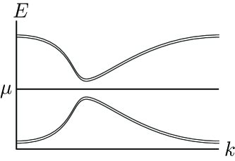
Figure 2: Schematic band structure that leads to vanishing $\alpha_{G}$. The bands below the chemical potential are degenerate with energy $E^{\rm v}_{\mathbf{k}}$, while the bands above the chemical potential have energy $E^{\rm c}_{\mathbf{k}}=\mathrm{const}.-E^{\rm v}_{\mathbf{k}}$.

Most model Hamiltonians discussed in the literature that access the topological insulator phase,Fu et al. (2007); Qi et al. (2008); Essin et al. (2009); Hosur et al. (2009); Li et al. (2009) as well as the Dirac Hamiltonian (in the context of which the axion electrodynamics was first discussedWilczek (1987)), can be defined in terms of a Clifford algebra, foo (3) and this ensures that the dispersions are degenerate and reflection symmetric. The only exception of which we are aware is the model of Guo and Franz on the pyrochlore lattice, which has four orbitals per unit cell.Guo and Franz (2009) The topological insulator phase itself will not have a contribution from $\alpha_{G}$, since it is $T$-invariant, and so the Guo and Franz model will not show such a response; however, the addition of any $T$-breaking perturbation to their model should produce off-diagonal magnetoelectric responses.

Finally, there is a simple mathematical condition that will cause $\alpha_{G}$ to vanish. Namely, $\alpha_{G}$ decreases as the gap becomes large without changing the wave functions, and in the limit of infinite bulk gap the only magnetoelectric response comes from the Chern-Simons part, which is not sensitive to the energies and depends only on the electron wave functions.

II.4 Is the Chern-Simons contribution physically distinct?

Apart from the ambiguity in $\alpha_{CS}$ that is not present in $\alpha_{G}$, there seems to be no real physical distinction between the two terms of the linear magnetoelectric response. We discuss two aspects that relate to this observation below.

Localized vs. itinerant contributions

The ambiguity in $\theta_{CS}$ can be interpreted as a manifestation of the fact that bulk quantities cannot determine the surface quantum Hall conductance, since a two-dimensional quantum Hall layer could appear on a surface independent of bulk properties. This suggests, perhaps, that the Chern-Simons term appears only in bulk systems with extended wave functions, and is a consequence of the itinerant electrons, while $\alpha_{G}$ is a localized molecule-like contribution. However, this turns out not to be the case.

Consider a periodic array of isolated molecules, which is an extreme limit of the class of crystalline insulators. Such a system has flat bands, with energies equal to the energies of the molecular states, since the electrons cannot propagate. It is certainly possible to construct a molecular system where all the unoccupied states have one energy and all the occupied states have another, by tuning the potentials. In this case $\alpha_{G}$ will vanish. However, such a molecule can still display a magnetoelectric response; it will therefore have to be given by $\alpha_{CS}$ (and so restricted to diagonal responses). For example, consider the “molecule” of Fig. (3) with the shape of a regular tetrahedron. If the two low-energy levels are occupied, the magnetoelectric response is

$$\frac{\partial P^{i}}{\partial B^{j}}=\pm\delta^{i}_{j}\frac{1}{\sqrt{6}}\frac{e^{2}}{\hslash},$$

where $P^{i}$ here is the electric dipole moment divided by the volume of the tetrahedron; the sign of the polarizability reverses when the complex phases are reversed. This shows that the Chern-Simons term does not require delocalized orbitals.

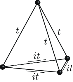
Figure 3: A tetrahedral tight-binding molecule for spinless electrons, with one orbital per site and complex hoppings. The hopping integrals are all equal, except that those around one face have a phase of $i$ relative to the other three. There are then two pairs of degenerate levels.

Additivity

Another argument against distinguishing between the Chern-Simons part and the rest of the susceptibility is based on band additivity. When interactions are not taken into account, each occupied band can be regarded as an independent physical system (at least if there are no band crossings). Applying a magnetic field causes each band $n$ to become polarized by a certain amount $\mathbf{P}_{n}$, and so the net polarization should be $\mathbf{P}=\sum_{n}\mathbf{P}_{n}$. The Pauli exclusion principle does not lead to any “interactions” between pairs of bands, because the polarization (like any single-body operator) can be written as the sum of the mean polarization in each of the orthonormal occupied states.

Now the Chern-Simons form does not look particularly additive in this sense, and is not by itself. Because it is the trace of a matrix product in the occupied subspace, it necessarily involves matrix elements between different occupied states, while an additive formula would not. Nevertheless, $\alpha_{G}$ and $\alpha_{CS}$ are together additive, as can be seen most simply in Eq. (54), where the two terms combine into a single sum over occupied bands. In terms of $\alpha_{G}$ and $\alpha_{CS}$ separately, one finds that when the values of $\alpha_{G}$, assuming just band 1 or 2 is occupied, are added together, some terms occur that are not present in the expression for $\alpha_{G}(1+2)$ (where both bands are occupied), and vice-versa. Using Eqs. (56c) and (56d) we see, in fact, that $\alpha_{G}$ is a sum of contributions which depend on three bands, as $\alpha_{G}=\sum_{n,m,m^{\prime}}C(n;m,m^{\prime})+\sum_{n,n^{\prime},m}D(n,n^{\prime};m)$. Terms such as $C(1;2,m^{\prime})$ are not present in the expression for $\alpha_{G}(1+2)$. (Likewise $D(1,2;m)$ appears in $\alpha_{G}(1+2)$ but not in $\alpha_{G}(1)$ and $\alpha_{G}(2)$.) Adding up the discrepancies, one finds that the energy-denominators all cancel, and the non-diagonal terms from the Chern-Simons form appear!

Seemingly paradoxical is the fact that for band structures satisfying the degeneracy and reflection conditions of the last subsection, the magnetoelectric susceptibility is given by the Chern-Simons term alone, which does not seem to be additive. However, the additivity property applies only to bands that do not cross. It does not make any sense to ask whether the susceptibility is the sum over the susceptibilities for the systems in which just one of the degenerate bands is occupied, since those systems are not gapped.

III The OMP as currents in response to Chemical Changes

Now we will tackle the problem of deriving the formula for the OMP $\alpha$ discussed in the last section. There are two impediments we need to overcome, a physical one, and a more technical one (which we will overcome starting from an insight of Levinson).Levinson (1970)

In order to determine $\alpha$, we would like to carry out a thought experiment in which a crystal is exposed to appropriate electromagnetic fields. For specificity, we will apply a uniform magnetic field. To make the calculation of the response clean, we wish to deal with an infinite crystal. Then the polarization does not simply reduce to the first moment of the charge density,King-Smith and Vanderbilt (1993) so we will instead have to calculate the current or charge distribution induced by the fields, and then use Eq. (I) to deduce $\alpha$. If both the crystal and the electromagnetic fields are independent of space and time, there is no macroscopic charge or current density. We will assume spatial uniformity, so that there are two choices for how to proceed. Either the magnetic field can be varied in time or the crystal parameters, and thus $\alpha$, can be varied. In either case, we measure the current that flows through the bulk and try to determine $\alpha$. As ever, the diagonal response $\alpha_{\theta}$ is the most difficult to capture: while either time-dependent experiment can be used to determine $\tilde{\alpha}$, only the latter approach sheds light on the value of $\alpha_{\theta}$.

To see why $\alpha_{\theta}$ can be determined only in this way (given that we want to work with a spatially homogeneous geometry), let us discuss how currents flow through the crystal. The necessity of varying the crystal in time can be deduced from Maxwell’s equations (see below) but we will give a more intuitive discussion here. Suppose that $\tilde{\alpha}=0$. Then in an applied magnetic field there is a polarization $\mathbf{P}=\alpha_{\theta}{\mathbf{B}}$; thus the crystal gets charged at the surface. As the magnetic field is turned on, this surface charge has to build up (charge density $\hat{\mathbf{n}}\cdot\mathbf{P}$). This occurs entirely due to flows of charge along the surface. Suppose, for example, that the sample is a cylinder (radius $R$) with the magnetic field along its $z$ axis, as illustrated in Fig. 4(a).

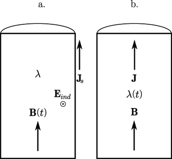
Figure 4: As outlined in the text, (a) turning on a magnetic field produces a macroscopic polarization through the flow of surface currents, while (b) varying the crystal Hamiltonian in the presence of a fixed magnetic field produces a polarization through the flow of current through the bulk.

Then an electric field ${\mathbf{E}}_{\mathrm{ind}}=-\dot{B}R\hat{\bm{\phi}}/2$ is induced at the surface according to Faraday’s law. Besides being the magnetoelectric response, $\theta$ also represents the Hall coefficient for surface currents. Therefore, a current of $J_{s}=\alpha_{\theta}\dot{B}R/2$ flows to the top of the cylinder, adding up to a surface charge of $2\pi R\int\!J_{s}(t)dt=\alpha_{\theta}B_{f}\pi R^{2}$ and producing the entire polarization $\alpha_{\theta}B_{f}$. No current flows through the bulk! In fact, the Hall conductance on the circular face produces a radial current as well, so that the charge distributes over the surface rather than just accumulating in a ring. Note that the surface current grows with the radius of the cylinder. This sounds like a nonlocal response, but it can be understood as follows: the electric field is determined by the non-local Faraday law, but the crystal’s response to the electric field (namely, the surface current) is local.

The current distribution can be understood directly from Maxwell’s equations: there are two contributions to the bulk current, $\partial_{t}\mathbf{P}$ and $\mathrm{curl}\ \mathbf{M}$. The polarization is $\alpha_{\theta}\mathbf{B}$ while the magnetization is indirectly produced by the induced electric field, $\alpha_{\theta}\mathbf{E}_{\mathrm{ind}}$. The two contributions thus cancel by Faraday’s law in the bulk: $\mathbf{J}_{b}^{\mathrm{bulk}}=\alpha_{\theta}(\partial_{t}\mathbf{B}+\mathrm{curl}\ \mathbf{E})=0$. There is a surface current because $\alpha_{\theta}$ is discontinuous there.

On the other hand, if $\theta$ changes in time, while the magnetic field is time-independent (as in Fig. 4b), the polarization at the ends of the cylinder builds up entirely by means of flows of charge through the bulk. Surface flows cannot be large enough to explain the net polarization in this situation. Since there is no induced electric field, the surface current is just proportional to the lateral surface area and is negligible compared to the bulk current. Therefore the bulk current is equal to $(\partial_{t}\alpha_{\theta})B$ and can be integrated to give $\alpha_{\theta}B$.

For the other component of the OMP, $\tilde{\alpha}$, either thought experiment can be used. The simplest approach, however, is still the crystal-variation method, since the surface currents are negligible in that case, foo (4) and in any case this method allows us to find all the components of $\alpha$ simultaneously.

Difficulties with the operator ${\mathbf{r}}$ and uniform magnetic fields

There are two technical difficulties in the theory. First, the operator ${\mathbf{r}}$ has unbounded matrix elements and thus the matrix elements of the magnetic dipole moment $(e/4)(\mathbf{v}\times{\mathbf{r}}-{\mathbf{r}}\times\mathbf{v})$ are not well-defined. This rules out the straightforward use of perturbation theory to calculate the electric dipole moment of an infinite crystal in a uniform magnetic field. Second, if we consider a crystal in a uniform magnetic field, Bloch’s theorem does not hold. Although the magnetic field is uniform, the vector potential that appears in the Hamiltonian depends on ${\mathbf{r}}$.

We avoid the problems of ${\mathbf{r}}$ as follows. The key idea is to work with the ground state density matrix, rather than wave functions. The individual eigenstates change drastically when a magnetic field, no matter how small, is applied (consider the difference between a plane wave and a localized Landau level). However, the density matrix of an insulator summed over the occupied bands only changes by a small amount when $\mathbf{B}$ is applied; over short distances the magnetic field cannot have a strong effect (even in the example of Landau levels), and the density matrix has only short-range correlations because it describes an insulating state. More technically, we show (subsection III.1) that the broken translation invariance of any single-body operator $\mathcal{O}$ (such as the density matrix) can be dealt with by factoring out an Aharonov-Bohm-like phase from its matrix $\mathcal{O}_{{\mathbf{r}}_{1}{\mathbf{r}}_{2}}$. This solves the problem of the nonuniform gauge field and leads to expressions that depend only on differences between $\mathbf{r}$’s. In addition, since the exponentially decaying ground-state density matrix appears multiplying every expression, the factors of $\mathbf{r}_{1}-\mathbf{r}_{2}$ are suppressed.

The calculation then proceeds as follows. First, using the symmetries of the electron Hamiltonian in a uniform magnetic field, we find how the density matrix changes in a weak magnetic field. Next we compute the current response to an adiabatic variation of the crystal Hamiltonian. Finally, we show that this current can be expressed as a total time derivative, and therefore can be integrated to give the polarization; at linear order in ${\mathbf{B}}$ we can read off the coefficients, the magnetoelectric tensor $\alpha$.

III.1 Single-body operators for a uniform magnetic field

Recall the form of the Schrödinger Hamiltonian for a single electron in a crystal and under the influence of a magnetic field,

$$H_{S}(\mathbf{p},{\mathbf{r}})=\frac{1}{2m}\left[\mathbf{p}-e\mathbf{A}({\mathbf{r}})\right]^{2}+V({\mathbf{r}}),$$ (10)

where $V({\mathbf{r}}+\mathbf{R})=V({\mathbf{r}})$ for lattice vectors $\mathbf{R}$. The necessity of using the vector potential $\mathbf{A}$ seems at first to spoil the lattice translation symmetry one would expect in a uniform magnetic field. However, as noted by BrownBrown (1964) and Zak,Zak (1964) a more subtle form of translation symmetry remains. In particular, choosing the gauge

$$\mathbf{A}=\frac{1}{2}{\mathbf{B}}\times{\mathbf{r}},$$ (11)

the Hamiltonian has “magnetic translation symmetry”:

$$H_{S}(\mathbf{p},{\mathbf{r}}+\mathbf{R})=e^{ie{\mathbf{B}}\cdot(\mathbf{R}\times{\mathbf{r}})/2\hslash}H_{S}(\mathbf{p},{\mathbf{r}})e^{-ie{\mathbf{B}}\cdot(\mathbf{R}\times{\mathbf{r}})/2\hslash}.$$ (12)

This condition defines magnetic translation symmetry for general single-body operators. Any operator $\mathcal{O}$ possessing this symmetry can be written in the position basis as

$$\mathcal{O}_{{\mathbf{r}}_{1}{\mathbf{r}}_{2}}=\bar{\mathcal{O}}_{{\mathbf{r}}_{1}{\mathbf{r}}_{2}}e^{-ie{\mathbf{B}}\cdot({\mathbf{r}}_{1}\times{\mathbf{r}}_{2})/2\hslash},$$ (13a)

where $$\bar{\mathcal{O}}$$ has lattice translation invariance,

$$\bar{\mathcal{O}}_{{\mathbf{r}}_{1}+\mathbf{R},{\mathbf{r}}_{2}+\mathbf{R}}=\bar{\mathcal{O}}_{{\mathbf{r}}_{1}{\mathbf{r}}_{2}}.$$ (13b)

Note that the phase is just $(ie/\hslash)\int d\bm{\ell}\cdot\mathbf{A}$ calculated along the straight line from ${\mathbf{r}}_{2}$ to ${\mathbf{r}}_{1}$, which agrees with the intuition that comes from writing the second-quantized form of the operator,

$$\mathcal{O}=\int\!d^{3}r_{1}d^{3}r_{2}\,\bar{\mathcal{O}}_{{\mathbf{r}}_{1}{\mathbf{r}}_{2}}c^{\dagger}_{{\mathbf{r}}_{1}}e^{-ie{\mathbf{B}}\cdot({\mathbf{r}}_{1}\times{\mathbf{r}}_{2})/2\hslash}c_{{\mathbf{r}}_{2}}.$$ (14)

This argument shows how to couple general Hamiltonians to uniform fields: $H=\exp[(ie/\hbar)\int_{\mathbf{r}_{2}}^{\mathbf{r}_{1}}d\bm{\ell}\cdot\mathbf{A}][H_{0\mathbf{r}_{1}\mathbf{r}_{2}}+H^{\prime}_{\mathbf{r}_{1}\mathbf{r}_{2}}(B)]$. The vector potential appears explicitly only in $\mathbf{A}$, while $H^{\prime}(B)$ gives the rest of the dependence on the magnetic field. The Schrödinger Hamiltonian (10) is obtained if we take

$$\bar{H}_{0,{\mathbf{r}}_{1}{\mathbf{r}}_{2}}=\left[-\frac{\hslash^{2}}{2m}\nabla^{2}_{{\mathbf{r}}_{2}}+V({\mathbf{r}}_{2})\right]\delta^{(3)}({\mathbf{r}}_{2}-{\mathbf{r}}_{1}).$$ (15)

and set $H^{\prime}=0$. Our results also apply to tight-binding models. We introduce $H^{\prime}$ to capture the possibility that in a tight-binding model the hoppings will not be rectilinear, and hence that the phases in Eq. (14) do not capture the full field dependence of the Hamiltonian.

III.2 The ground state density operator

We find it convenient to work with the one-body density matrix $\rho^{g}$, or equivalently the projector onto the occupied states, whenever possible, because it is a basis-independent object. Also, in an insulator, $\rho^{g}_{{\mathbf{r}}_{1}{\mathbf{r}}_{2}}$ is exponentially suppressed in the distance $|{\mathbf{r}}_{2}-{\mathbf{r}}_{1}|$, which tempers the divergences that arise from the unboundedness of ${\mathbf{r}}$.Kohn (1964) In any case, if the ground state is translationally symmetric, the structure described above will apply to $\rho_{g}$ and we can be sure that the density matrix has translational symmetry apart from a phase:

$$\rho^{g}_{{\mathbf{r}}_{1}{\mathbf{r}}_{2}}=\bar{\rho}^{g}_{{\mathbf{r}}_{1}{\mathbf{r}}_{2}}e^{-ie{\mathbf{B}}\cdot({\mathbf{r}}_{1}\times{\mathbf{r}}_{2})/2\hslash},$$ (16)

where $\bar{\rho}^{g}$ possesses the translation symmetry of the crystal lattice and hence should connect smoothly to the field-free density matrix. Hence we will write

$$\bar{\rho}^{g}=\rho_{0}+\rho^{\prime},$$ (17)

where $\rho_{0}$ is the density operator of the crystal in the absence of the magnetic field.

Density matrix perturbation theory: Now we have to calculate $\rho^{\prime}$, using a kind of perturbation theory that focuses on density matrices rather than wave functions, since the wave-functions suffer from the problems discussed above. This perturbation theory starts from two characteristic properties of the density matrix: it commutes with $H$, and for fermions at zero temperature it is a projection operator. The latter means that all states are either occupied or unoccupied, so the eigenvalues of the density operator are 0 and 1, which is formalized as

$$\rho^{g}\rho^{g}=\rho^{g}$$ (18)

(idempotency).Dirac (1931) Expressed in the position basis,

$$\rho^{g}_{{\mathbf{r}}_{1}{\mathbf{r}}_{3}} =\int d{\mathbf{r}}_{2}\rho^{g}_{{\mathbf{r}}_{1}{\mathbf{r}}_{2}}\rho^{g}_{{\mathbf{r}}_{2}{\mathbf{r}}_{3}}$$

$$\bar{\rho}^{g}_{{\mathbf{r}}_{1}{\mathbf{r}}_{3}} =\int d{\mathbf{r}}_{2}\bar{\rho}^{g}_{{\mathbf{r}}_{1}{\mathbf{r}}_{2}}\bar{\rho}^{g}_{{\mathbf{r}}_{2}{\mathbf{r}}_{3}}e^{-(ie/2\hslash){\mathbf{B}}\cdot({\mathbf{r}}_{1}\times{\mathbf{r}}_{2}+{\mathbf{r}}_{2}\times{\mathbf{r}}_{3}+{\mathbf{r}}_{3}\times{\mathbf{r}}_{1})}.$$ (19)

The exponent is just $-i\phi_{123}/\phi_{0}$, proportional to the magnetic flux through triangle 123, and the exponential can be expanded for small $B$. At first order this gives

$$\rho^{\prime}_{{\mathbf{r}}_{1}{\mathbf{r}}_{3}}=\int d{\mathbf{r}}_{2}[\rho^{\prime}_{{\mathbf{r}}_{1}{\mathbf{r}}_{2}}\rho_{0{\mathbf{r}}_{2}{\mathbf{r}}_{3}}+\rho_{0{\mathbf{r}}_{1}{\mathbf{r}}_{2}}\rho^{\prime}_{{\mathbf{r}}_{2}{\mathbf{r}}_{3}}\\ -\rho_{0{\mathbf{r}}_{1}{\mathbf{r}}_{2}}\rho_{0{\mathbf{r}}_{2}{\mathbf{r}}_{3}}\left(i\phi_{123}/\phi_{0}\right)].$$ (20)

The problem of the unbounded ${\mathbf{r}}$’s is resolved in this equation because the area $A_{123}$ of the triangle is finite and independent of the origin, and also suppressed by the factor of $\rho$.

Calculation of $\rho^{\prime}$: In the last term of Eq. (20), we can rewrite $2A_{123}={\mathbf{r}}_{1}\times{\mathbf{r}}_{2}+{\mathbf{r}}_{2}\times{\mathbf{r}}_{3}+{\mathbf{r}}_{3}\times{\mathbf{r}}_{1}=({\mathbf{r}}_{2}-{\mathbf{r}}_{1})\times({\mathbf{r}}_{3}-{\mathbf{r}}_{2})$ and then use $({\mathbf{r}}_{2}-{\mathbf{r}}_{1})\rho_{0{\mathbf{r}}_{1}{\mathbf{r}}_{2}}=[\rho_{0},{\mathbf{r}}]_{{\mathbf{r}}_{1}{\mathbf{r}}_{2}}$, etc., to obtain

$$(1-\rho_{0})\rho^{\prime}(1-\rho_{0})-\rho_{0}\rho^{\prime}\rho_{0}=-i\frac{e}{2\hslash}{\mathbf{B}}\cdot([\rho_{0},{\mathbf{r}}]\times[\rho_{0},{\mathbf{r}}]).$$ (21)

If we define

$$\bar{H}=H_{0}+H^{\prime},$$ (22)

then analogous manipulations (including $({\mathbf{r}}_{1}-{\mathbf{r}}_{2})H_{{\mathbf{r}}_{1}{\mathbf{r}}_{2}}=i\hslash\mathbf{v}_{{\mathbf{r}}_{1}{\mathbf{r}}_{2}}$) on the equation $[H,\rho^{g}]=0$ give

$$[\rho^{\prime},H_{0}]=\frac{e}{2}\mathbf{B}\cdot([\rho_{0},{\mathbf{r}}]\times\mathbf{v}-\mathbf{v}\times[\rho_{0},{\mathbf{r}}])-[\rho_{0},H^{\prime}].$$ (23)

Eqs. (21) and (23) have an intuitive meaning. The former equation determines the “interior” matrix elements of $\rho^{\prime}$, those between two occupied or two unoccupied states of the zero-field Hamiltonian. An perturbation with the full crystal symmetry does not change the interior matrix elements of the density matrix because of the exclusion principle.McWeeny (1962) In our case, however, multiplying $\rho_{0}$ by the phase $e^{(ie/2\hslash){\mathbf{B}}\cdot{\mathbf{r}}_{1}\times{\mathbf{r}}_{2}}$ gives a density matrix with the correct magnetic translation symmetry, but also changes the momentum of the states and so results in a small probability for states to be douby occupied. Therefore $\rho^{\prime}$ must correct for this “violation of the exclusion principle.” On the other hand Eq. (23) determines the “cross-gap” matrix elements of $\rho^{\prime}$ (those between unoccupied and occupied states). These matrix elements capture the expected “transitions across the gap” induced by the field. The rest of this section is devoted to calculating all these matrix elements. The results are given in Eqs. (III.2) and (28); the derivations could be skipped on a first reading.

Calculation of $\rho^{\prime}$. Precisely speaking, Eq. (21) gives the matrix elements of $\bar{\rho}^{g}$ between pairs of occupied ($n$ and $n^{\prime}$) or unoccupied ($m$ and $m^{\prime}$) states:

$$\langle\psi_{n{\mathbf{k}}}|\bar{\rho}^{g}|\psi_{n^{\prime}{\mathbf{k}}}\rangle =\delta_{nn^{\prime}}-\frac{e}{4\hslash}B^{j}\epsilon_{jab}{\cal F}^{ab}_{nn^{\prime}}({\mathbf{k}})$$

$$\langle\psi_{m{\mathbf{k}}}|(1-\bar{\rho}^{g})|\psi_{m^{\prime}{\mathbf{k}}}\rangle =\delta_{mm^{\prime}}-\frac{e}{4\hslash}B^{j}\epsilon_{jab}\check{{\cal F}}^{ab}_{mm^{\prime}}({\mathbf{k}}),$$ (24)

where ${\cal F}$ is the non-Abelian Berry curvature associated with the occupied bands,

$${\cal F}^{ab}_{nn^{\prime}} =i\langle u_{n{\mathbf{k}}}|\partial^{a}\mathcal{P}_{\mathbf{k}}\partial^{b}\mathcal{P}_{\mathbf{k}}-\partial^{b}\mathcal{P}_{\mathbf{k}}\partial^{a}\mathcal{P}_{\mathbf{k}}|u_{n^{\prime}{\mathbf{k}}}\rangle$$

$$=\partial^{a}{\cal A}^{b}_{nn^{\prime}}-\partial^{b}{\cal A}^{a}_{nn^{\prime}}-i[{\cal A}^{a},{\cal A}^{b}]_{nn^{\prime}},$$ (25)

and $\check{{\cal F}}$ is the corresponding quantity for the unoccupied bands. To derive these relations, we use

$$\rho^{g}=\int_{\rm BZ}\!\frac{d^{3}k}{(2\pi)^{3}}e^{i{\mathbf{k}}\cdot{\mathbf{r}}}\mathcal{P}_{{\mathbf{k}}}e^{-i{\mathbf{k}}\cdot{\mathbf{r}}}$$ (26)

where $\mathcal{P}=\sum_{n\,\mathrm{occ}}|u_{n{\mathbf{k}}}\rangle\langle u_{n{\mathbf{k}}}|$ is the projector onto filled bands at ${\mathbf{k}}$. This gives

$$i[\rho^{g},{\mathbf{r}}] =\int_{\rm BZ}\!\frac{d^{3}k}{(2\pi)^{3}}e^{i{\mathbf{k}}\cdot{\mathbf{r}}}(\bm{\nabla}_{{\mathbf{k}}}\mathcal{P}_{{\mathbf{k}}})e^{-i{\mathbf{k}}\cdot{\mathbf{r}}}$$

$$=\int_{\rm BZ}\!\frac{d^{3}k}{(2\pi)^{3}}e^{i{\mathbf{k}}\cdot{\mathbf{r}}}\not{\mathbf{r}}_{\mathbf{k}}e^{-i{\mathbf{k}}\cdot{\mathbf{r}}}$$ (27)

after discarding a total derivative. The notation $\not\!\!{\mathbf{r}}=\bm{\nabla}_{{\mathbf{k}}}\mathcal{P}$ was introduced in Eq. (5).

By contrast, Eq. (23) describes to what extent $\bar{\rho}^{g}$ fails to commute with $H_{0}$, the crystal Hamiltonian, and gives the matrix elements of $\rho^{\prime}$ between occupied and unoccupied states. In this sense it is analogous to the more usual results for density-matrix perturbation theory.McWeeny (1962) In the basis of unperturbed energy eigenstates,

$$\langle\psi_{n{\mathbf{k}}}|\rho^{\prime}|\psi_{m{\mathbf{k}}}\rangle=i\frac{e}{2\hslash}B^{j}\epsilon_{jab}\frac{\langle u_{n{\mathbf{k}}}|\{\partial^{a}\mathcal{P}_{{\mathbf{k}}},\partial^{b}H_{{\mathbf{k}}}\}|u_{m{\mathbf{k}}}\rangle}{E_{n{\mathbf{k}}}-E_{m{\mathbf{k}}}}\\ +\frac{\langle u_{n{\mathbf{k}}}|H^{\prime}_{{\mathbf{k}}}|u_{m{\mathbf{k}}}\rangle}{E_{n{\mathbf{k}}}-E_{m{\mathbf{k}}}}.$$ (28)

Recall that $\hslash v^{b}=\partial^{b}H_{{\mathbf{k}}}$ and that $H^{\prime}$ is introduced only to capture unusual situations such as tight-binding models with non-straight hoppings, and vanishes for the continuum problem. Eqs. (III.2) and (28) are the key technical results of this formalism, good to linear order in the magnetic field.

III.3 Adiabatic current

Now we need to calculate the current as the Hamiltonian is changed slowly as a function of time, as in the ordinary theory of polarization.Resta (1992); King-Smith and Vanderbilt (1993) We have to be careful, however, since the current vanishes in the zero-order adiabatic ground state described by density matrix $\rho^{g}(t)$. It is necessary to go to first order in adiabatic perturbation theory, which takes account of the fact that the true dynamical density matrix $\rho(t)$ has an extra contribution proportional to $dH/dt=\dot{H}$. However, once the current has been expressed in terms of $\dot{\rho}$, which is proportional to $\dot{H}$, the distinction is no longer important and the adiabatic approximation can be made.

Preparing for the adiabatic approximation: We can write the current as

$$\mathbf{J}(t)=\frac{e}{\Omega}\mathrm{Tr}\rho(t)\mathbf{v}=\frac{e}{\Omega}\frac{i}{\hslash}\mathrm{Tr}\rho[H,{\mathbf{r}}]$$ (29)

where $\Omega$ is the crystal volume. Here $H$ is the full Hamiltonian including the magnetic field. By unitarity of time evolution, it remains a projector if the initial state describes filled bands only. The operator ${\mathbf{r}}$ appears here, but in a commutator. Since $\langle{\mathbf{r}}_{1}|[\mathcal{O},{\mathbf{r}}]|{\mathbf{r}}_{2}\rangle=({\mathbf{r}}_{2}-{\mathbf{r}}_{1})\mathcal{O}_{{\mathbf{r}}_{1}{\mathbf{r}}_{2}}$, such expressions do not suffer from the difficulties of an “unprotected” ${\mathbf{r}}$, namely its unboundedness. We can only use cyclicity of the trace to the extent that this property can be preserved. In particular, the expression $\mathrm{Tr}\,{\mathbf{r}}[\rho,H]$, which seems formally equivalent to Eq. (29), poses problems, but

$$\mathbf{J}(t)=\frac{e}{\Omega}\frac{i}{\hslash}\mathrm{Tr}[\rho,[\rho,\mathbf{r}]][\rho,H]$$ (30)

does not. This expression can be derived from Eq. (29) using again the idempotency of $\rho$ ($\rho\rho=\rho$). Using the equation of motion for the density matrix,

$$i\hbar\dot{\rho}(t)=[H(t),\rho(t)],$$ (31)

and making the approximation $\rho\approx\rho^{g}$ on the right-hand side at this stage, the current becomes

$$\mathbf{J}=\frac{e}{\Omega}\int\!d{\mathbf{r}}_{1}d{\mathbf{r}}_{2}d{\mathbf{r}}_{3}({\mathbf{r}}_{1}-2{\mathbf{r}}_{2}+{\mathbf{r}}_{3})\rho^{g}_{{\mathbf{r}}_{1}{\mathbf{r}}_{2}}\rho^{g}_{{\mathbf{r}}_{2}{\mathbf{r}}_{3}}\dot{\rho}^{g}_{{\mathbf{r}}_{3}{\mathbf{r}}_{1}}.$$ (32)

Magnetic field dependence of the current: The considerations given in the last subsection make the integrand

$$\rho^{g}_{{\mathbf{r}}_{1}{\mathbf{r}}_{2}}\rho^{g}_{{\mathbf{r}}_{2}{\mathbf{r}}_{3}}\dot{\rho}^{g}_{{\mathbf{r}}_{3}{\mathbf{r}}_{1}}=\bar{\rho}^{g}_{{\mathbf{r}}_{1}{\mathbf{r}}_{2}}\bar{\rho}^{g}_{{\mathbf{r}}_{2}{\mathbf{r}}_{3}}\dot{\bar{\rho}}^{g}_{{\mathbf{r}}_{3}{\mathbf{r}}_{1}}e^{-i\phi_{123}/\phi_{0}},$$ (33)

where, again, $\phi_{123}={\mathbf{B}}\cdot({\mathbf{r}}_{1}\times{\mathbf{r}}_{2}+{\mathbf{r}}_{2}\times{\mathbf{r}}_{3}+{\mathbf{r}}_{3}\times{\mathbf{r}}_{1})/2$ is the magnetic flux through the triangle with vertices ${\mathbf{r}}_{1}{\mathbf{r}}_{2}{\mathbf{r}}_{3}$ and does not suffer from the pathologies of ${\mathbf{r}}$ itself, which allows us to expand $e^{-i\phi_{123}/\phi_{0}}=1-i\phi_{123}/\phi_{0}$ to lowest order in $B$ (recall again that the matrix elements of $\rho$ are exponentially suppressed with distances).

Recalling our division $\bar{\rho}^{g}=\rho_{0}+\rho^{\prime}$ where $\rho^{\prime}$ is of first order in the magnetic field, Eq. (32) becomes

$$\mathbf{J}=\frac{e}{\Omega}\int d{\mathbf{r}}_{1}d{\mathbf{r}}_{2}d{\mathbf{r}}_{3}({\mathbf{r}}_{1}-2{\mathbf{r}}_{2}+{\mathbf{r}}_{3})\bigg{[}\rho_{0{\mathbf{r}}_{1}{\mathbf{r}}_{2}}\rho_{0{\mathbf{r}}_{2}{\mathbf{r}}_{3}}\dot{\rho}^{\prime}_{{\mathbf{r}}_{3}{\mathbf{r}}_{1}}\\ +\rho^{\prime}_{{\mathbf{r}}_{1}{\mathbf{r}}_{2}}\rho_{0{\mathbf{r}}_{2}{\mathbf{r}}_{3}}\dot{\rho}_{0{\mathbf{r}}_{3}{\mathbf{r}}_{1}}+\rho_{0{\mathbf{r}}_{1}{\mathbf{r}}_{2}}\rho^{\prime}_{{\mathbf{r}}_{2}{\mathbf{r}}_{3}}\dot{\rho}_{0{\mathbf{r}}_{3}{\mathbf{r}}_{1}}\\ -i\frac{\phi_{123}}{\phi_{0}}\rho_{0{\mathbf{r}}_{1}{\mathbf{r}}_{2}}\rho_{0{\mathbf{r}}_{2}{\mathbf{r}}_{3}}\dot{\rho}_{0{\mathbf{r}}_{3}{\mathbf{r}}_{1}}\bigg{]}$$ (34)

at first order. The rest of the calculation involves substituting the expressions for the magnetic-field dependence of $\rho^{g}$ obtained earlier, and integrating the result to obtain $\alpha$. The energy-dependent part of $\alpha$, namely $\alpha_{G}$, will come from the mixing of the occupied and unoccupied bands, Eq. (28). The Chern-Simons term will come from the “exclusion-principle–correcting” terms, Eq. (III.2), as well as the $\phi_{123}$ term in the previous equation.

Integrating the results:

The four terms in the current can be collected and rearranged into the form

$$\mathbf{J}=\mathbf{J}_{G}+\mathbf{J}_{CS1}+\mathbf{J}_{CS2}$$ (35a)

and integrated with respect to time as follows. The first term in Eq. (34) can be rewritten with $$\rho_{0{\mathbf{r}}_{1}{\mathbf{r}}_{2}}\rho_{0{\mathbf{r}}_{2}{\mathbf{r}}_{3}}\dot{\rho}^{\prime}_{{\mathbf{r}}_{3}{\mathbf{r}}_{1}}=\partial_{t}(\rho_{0{\mathbf{r}}_{1}{\mathbf{r}}_{2}}\rho_{0{\mathbf{r}}_{2}{\mathbf{r}}_{3}}\rho^{\prime}_{{\mathbf{r}}_{3}{\mathbf{r}}_{1}})-\dot{\rho}_{0{\mathbf{r}}_{1}{\mathbf{r}}_{2}}\rho_{0{\mathbf{r}}_{2}{\mathbf{r}}_{3}}\rho^{\prime}_{{\mathbf{r}}_{3}{\mathbf{r}}_{1}}-\rho_{0{\mathbf{r}}_{1}{\mathbf{r}}_{2}}\dot{\rho}_{0{\mathbf{r}}_{2}{\mathbf{r}}_{3}}\rho^{\prime}_{{\mathbf{r}}_{3}{\mathbf{r}}_{1}}$$ and combined with the next two terms to give

$$\mathbf{J}_{G} =\frac{e}{\Omega}\partial_{t}\mathrm{Tr}[\rho_{0},{\mathbf{r}}][\rho^{\prime},\rho_{0}]$$ (35b)

$$\mathbf{J}_{CS1} =-3\frac{e}{\Omega}\mathrm{Tr}\rho^{\prime}[\dot{\rho}_{0},[\rho_{0},{\mathbf{r}}]],$$ (35c)

while the final term in Eq. (34) (i.e., the term involving $$\phi_{123}$$) becomes

$$\mathbf{J}_{CS2}=-i\frac{e^{2}}{2\hslash\Omega}B^{j}\epsilon_{jab}\mathrm{Tr}[\rho_{0},{\mathbf{r}}][\rho_{0},r^{a}][r^{b},\dot{\rho}_{0}]+\mathrm{c.c.}$$ (35d)

upon rewriting

$$({\mathbf{r}}_{1}-2{\mathbf{r}}_{2}+{\mathbf{r}}_{3})({\mathbf{r}}_{1}\times{\mathbf{r}}_{2}+{\mathbf{r}}_{2}\times{\mathbf{r}}_{3}+{\mathbf{r}}_{3}\times{\mathbf{r}}_{1})\\ =({\mathbf{r}}_{1}-{\mathbf{r}}_{2})[({\mathbf{r}}_{1}-{\mathbf{r}}_{3})\times({\mathbf{r}}_{2}-{\mathbf{r}}_{3})]\\ +({\mathbf{r}}_{3}-{\mathbf{r}}_{2})[({\mathbf{r}}_{1}-{\mathbf{r}}_{2})\times({\mathbf{r}}_{1}-{\mathbf{r}}_{3})].$$ (36)

The total derivative term $\mathbf{J}_{G}$ [Eq. (35b)] can be written

$$J^{i}_{G}=\partial_{t}(\alpha_{G})^{i}_{j}B^{j}$$ (37)

with $\alpha_{G}$ as given in Eq. (5b),

$$(\alpha_{G})^{i}_{j}=\frac{e^{2}}{\hslash}\mathrm{Re}\negthickspace\sum_{\begin{subarray}{c}n\,\mathrm{occ}\\ m\,\mathrm{unocc}\end{subarray}}\negthickspace\frac{\langle n|\partial^{i}\mathcal{P}|m\rangle\langle m|\epsilon_{jab}\{\partial^{a}H,\partial^{b}\mathcal{P}\}|n\rangle}{E_{n}-E_{m}}\\ +2e\,\mathrm{Im}\negthickspace\sum_{\begin{subarray}{c}n\,\mathrm{occ}\\ m\,\mathrm{unocc}\end{subarray}}\negthickspace\frac{\langle n|\partial^{i}\mathcal{P}|m\rangle\langle m|\partial H^{\prime}/\partial B^{j}|n\rangle}{E_{n}-E_{m}},$$ (38)

where the BZ integral and the dependence on ${\mathbf{k}}$ have been suppressed, and $|n\rangle=|u_{n}\rangle$, etc. This result follows immediately upon taking the trace in the basis of energy eigenstates. Matrix elements of $[\rho_{0},r^{i}]$ appear as $\not\!r^{i}_{{\mathbf{k}}}=\partial^{i}\mathcal{P}_{k}$, from Eq. (III.2), and the cross-gap matrix elements of $\rho^{\prime}$ in are given in Eq. (28). Note that since $\mathbf{J}_{G}$ is a total time derivative, $\alpha_{G}$ is uniquely defined for a given Hamiltonian (this assumes the existence of a reference Hamiltonian with $\alpha_{G}=0$, that is, the existence of a topologically trivial, time-reversal-invariant band insulator).

In $\mathbf{J}_{CS2}$ [Eq. (35d)], we can replace $r\rightarrow[[r,\rho_{0}],\rho_{0}]$ in the third commutator. This has the same cross-gap matrix elements as $r$; the interior matrix elements do not contribute to the trace because the other three factors, $\dot{\rho}_{0}$ and two components of $[\rho_{0},r^{i}]$, have only cross-gap matrix elements. Then

$$\mathbf{J}_{CS2}=i\frac{e^{2}}{2\hslash\Omega}B^{j}\epsilon_{jab}\mathrm{Tr}[\rho_{0},{\mathbf{r}}][\rho_{0},r^{a}][[[\rho_{0},r^{b}],\rho_{0}],\dot{\rho}_{0}]+\mathrm{c.c.}$$

or

$$\mathbf{J}_{CS2}=-\frac{e^{2}}{2\hslash}B^{j}\epsilon_{jab}\mathrm{Tr}\bm{\nabla}_{k}\mathcal{P}_{{\mathbf{k}}}\partial^{a}\mathcal{P}_{{\mathbf{k}}}[[\partial^{b}\mathcal{P}_{{\mathbf{k}}},\mathcal{P}_{{\mathbf{k}}}],\dot{\mathcal{P}}_{{\mathbf{k}}}]+\mathrm{c.c.},\\$$

where an integral over ${\mathbf{k}}$ is suppressed for brevity and the trace is taken in the Hilbert space at ${\mathbf{k}}$. Dropping the subscripts ${\mathbf{k}}$ everywhere, this can be expanded and rearranged to give

$$\mathbf{J}_{CS2}=\frac{e^{2}}{2\hslash}B^{j}\epsilon_{jab}\mathrm{Tr}\mathcal{P}\{[\bm{\nabla}\mathcal{P},\dot{\mathcal{P}}]\partial^{a}\mathcal{P}\partial^{b}\mathcal{P}\\ +2[\dot{\mathcal{P}},\partial^{b}\mathcal{P}][\bm{\nabla}\mathcal{P},\partial^{a}\mathcal{P}]\\ +3(\dot{\mathcal{P}}\partial^{b}\mathcal{P}\partial^{a}\mathcal{P}\bm{\nabla}\mathcal{P}+\partial^{b}\mathcal{P}\dot{\mathcal{P}}\bm{\nabla}\mathcal{P}\partial^{a}\mathcal{P})\}.$$ (39)

In manipulating these strings of projection operators and their derivatives, it is very useful to realize that derivatives of projectors only have cross-gap matrix elements: $\mathcal{P}\partial^{a}\mathcal{P}\mathcal{P}=\mathcal{Q}\partial^{a}\mathcal{P}\mathcal{Q}=0$, where $\mathcal{Q}=1-\mathcal{P}$ is the projector onto unoccupied bands. This means, for example, that $\mathcal{P}(\bm{\nabla}\mathcal{P})(\dot{\mathcal{P}})=\mathcal{P}(\bm{\nabla}\mathcal{P})\mathcal{Q}(\dot{\mathcal{P}})\mathcal{P}$.

To $\mathbf{J}_{CS2}$ we must add $\mathbf{J}_{CS1}$ [Eq. (35c)],

$$\mathbf{J}_{CS1}=\frac{3e^{2}}{2\hslash}B^{j}\epsilon_{jab}\mathrm{Tr}(\mathcal{P}-\mathcal{Q})[\dot{\mathcal{P}},\bm{\nabla}\mathcal{P}]\partial^{a}\mathcal{P}\partial^{b}\mathcal{P}\\ =\frac{3e^{2}}{2\hslash}B^{j}\epsilon_{jab}\mathrm{Tr}\mathcal{P}\{[\dot{\mathcal{P}},\bm{\nabla}\mathcal{P}]\partial^{a}\mathcal{P}\partial^{b}\mathcal{P}\\ -(\dot{\mathcal{P}}\partial^{b}\mathcal{P}\partial^{a}\mathcal{P}\bm{\nabla}\mathcal{P}+\partial^{b}\mathcal{P}\dot{\mathcal{P}}\bm{\nabla}\mathcal{P}\partial^{a}\mathcal{P})\},$$ (40)

to get

$$\mathbf{J}_{CS} =\mathbf{J}_{CS1}+\mathbf{J}_{CS2}$$

$$=\frac{e^{2}}{\hslash}B^{j}\epsilon_{jab}\mathrm{Tr}\mathcal{P}\{[\dot{\mathcal{P}},\bm{\nabla}\mathcal{P}]\partial^{a}\mathcal{P}\partial^{b}\mathcal{P}$$

$$\qquad+[\dot{\mathcal{P}},\partial^{b}\mathcal{P}][\bm{\nabla}\mathcal{P},\partial^{a}\mathcal{P}]\}.$$ (41)

By checking the different components explicitly one can see that this is

$$\mathbf{J}_{CS}={\mathbf{B}}\frac{e^{2}}{\hslash}\mathrm{Tr}\mathcal{P}\{[\dot{\mathcal{P}},\partial^{x}\mathcal{P}][\partial^{y}\mathcal{P},\partial^{z}\mathcal{P}]\\ +[\dot{\mathcal{P}},\partial^{y}\mathcal{P}][\partial^{z}\mathcal{P},\partial^{x}\mathcal{P}]+[\dot{\mathcal{P}},\partial^{z}\mathcal{P}][\partial^{x}\mathcal{P},\partial^{y}\mathcal{P}]\},$$ (42)

so we get the “topological current”

$$\mathbf{J}_{CS}=-{\mathbf{B}}\frac{e^{2}}{\hslash}\int_{\rm BZ}\!\frac{d^{3}k}{(2\pi)^{3}}\mathrm{tr}({\cal F}^{tx}{\cal F}^{yz}+{\cal F}^{ty}{\cal F}^{zx}+{\cal F}^{tz}{\cal F}^{xy}),$$ (43)

where the lower-case trace ($\mathrm{tr}$) is only over the occupied bands, and the Brillouin-zone integral has been restored.

It remains only to show that $\mathbf{J}_{CS}$ is a total time derivative that integrates to $\alpha_{CS}{\mathbf{B}}$. Allowing the indices to run over $t,x,y,z$, in that order (so that $\epsilon_{txyz}=+1$),

$$\mathbf{J}_{CS}=-{\mathbf{B}}\frac{e^{2}}{8\hslash}\int_{\rm BZ}\!\frac{d^{3}k}{(2\pi)^{3}}\epsilon_{abcd}\mathrm{tr}{\cal F}^{ab}{\cal F}^{cd}$$

$$=-{\mathbf{B}}\frac{e^{2}}{2\hslash}\epsilon_{abcd}\int_{\rm BZ}\!\frac{d^{3}k}{(2\pi)^{3}}\partial^{a}\mathrm{tr}\left(\mathcal{A}^{b}\partial^{c}\mathcal{A}^{d}-i\frac{2}{3}\mathcal{A}^{b}\mathcal{A}^{c}\mathcal{A}^{d}\right).$$ (44)

The derivatives with respect to $k_{x},k_{y},k_{z}$ will vanish when integrated over the Brillouin zone assuming that ${\cal A}$ is defined smoothly and periodically over the zone, leaving just

$$\mathbf{J}_{CS}\!=\!-{\mathbf{B}}\frac{e^{2}}{2\hslash}\partial_{t}\!\int_{\rm BZ}\!\frac{d^{3}k}{(2\pi)^{3}}\epsilon_{abc}\mathrm{tr}\!\left(\mathcal{A}^{a}\partial^{b}\mathcal{A}^{c}-i\frac{2}{3}\mathcal{A}^{a}\mathcal{A}^{b}\mathcal{A}^{c}\right),$$ (45)

where the indices now only run over $xyz$, as originally. This obviously gives $\alpha_{CS}$ as in Eq. (5c), completing the proof. It must be reiterated that this integral is not always entirely trivial. In particular, if the adiabatic evolution brings the crystal back to its initial Hamiltonian in a nontrivial way, the Brillouin zone integral need not return to its initial value because ${\cal A}$ is not uniquely defined. In other words, $\int dt\mathbf{J}_{CS}$ can be multivalued as a function of the Hamiltonian deformation parameters. However, the change can only be such that $\theta$ changes by an integer multiple of $2\pi$, as discussed in subsection II.2.

IV Summary

The theoretical calculation of the magnetoelectric polarizability in insulators presents a difficulty similar to that known well from the theory of polarization; both quantities suffer an inherent ambiguity in the bulk. The magnetoelectric polarizability adds another level of difficulty because the vector potential is unbounded and breaks lattice translation symmetry. However, we have developed a formalism that allows us to deal directly with a uniform magnetic field. In the appendix, we further show that a long-wavelength regularization of the vector potential together with a suitable generalization of the polarization (to deal with the broken crystal symmetry) provides a (relatively) simple, though less rigorous, way to compute the response function. The final expression for the OMP rederives known results for particular model systems and topological insulators and completes the picture with additional terms that have a relatively straightforward and intuitive interpretation. We hope that these results and the method of their derivation will be valuable for future work on magnetoelectric effects and topological electronic phases.

The authors gratefully acknowledge useful discussions with S. Coh, A. Malashevich and I. Souza. The work was supported by the Western Institute of Nanoelectronics (AME), DARPA OLE (AMT), NSF DMR-0804413 (JEM), and NSF DMR-0549198 (DV).

Appendix A Calculating the OMP using Static Polarization

As noted in the text, matrix elements of the operator $r$ are ill-behaved in a basis of extended, Bloch-like states. That problem was solved by working with the density operator $\rho$, whose matrix elements are exponentially suppressed with distance. Another approach is to use a Wannier-like basis of localized states. In this appendix, we take this approach to present an alternative derivation of the OMP.

The Bloch functions $\psi_{n{\mathbf{k}}}({\mathbf{r}})$ of the unperturbed crystal will evolve, under the application of a long-wavelength magnetic field $\mathbf{A}=\mathbf{A}_{0}\sin\mathbf{q}\cdot\mathbf{r}$, into the exact energy eigenfunctions $\Psi_{n{\mathbf{k}}}({\mathbf{r}})$. These no longer have a sharp crystal momentum ${\mathbf{k}}$, but may be expanded in a perturbation series in the unperturbed $\psi_{n{\mathbf{k}}}({\mathbf{r}})$. Then the analogue to the standard Wannier function $w_{n\mathbf{R}}({\mathbf{r}})$ for lattice vector $\mathbf{R}$ will be

$$W_{n\mathbf{R}}({\mathbf{r}}) =\frac{\Omega}{\sqrt{N}}\int_{\rm BZ}\!\frac{d^{3}k}{(2\pi)^{3}}\Psi_{n{\mathbf{k}}}({\mathbf{r}})e^{-i{\mathbf{k}}\cdot\mathbf{R}}$$

$$=w_{n\mathbf{R}}({\mathbf{r}})+\delta w_{n\mathbf{R}}({\mathbf{r}}),$$ (46)

where $\Omega$ is the volume of the crystal and $N$ is the number of unit cells. The Wannier orbitals centered at $\mathbf{R}$ become polarized when the magnetic field is applied, and this distortion gives a polarization density of

$$\delta\mathbf{P}(\mathbf{R})=\frac{1}{\Omega}\sum_{n\,\mathrm{occ}}\langle w_{n\mathbf{R}}|e{\mathbf{r}}|\delta w_{n\mathbf{R}}\rangle+\mathrm{c.c.}$$ (47)

Although it is not obvious that the bulk polarization appearing in Maxwell’s equations is the same as the polarization of a set of Wannier orbitals, this expression leads to Eq. (5). To ensure that the Wannier orbitals are localized, we will have to suppose that each band has a vanishing Chern number,Thouless (1984) so that the phase of $u_{n{\mathbf{k}}}$ can be chosen so that it is a periodic function of ${\mathbf{k}}$. In this case the unperturbed Wannier functions are localized, and (though there are usually subtleties in defining Wannier functions in a magnetic fields),Rashba et al. (1997) the regularization used here leads to localized orbitals. Presumably these arguments can be extended to the case where the total Chern number for all occupied bands $C^{ij}=\sum_{n\,\mathrm{occ}}\int_{\mathrm{BZ}}d^{3}k\mathcal{F}^{ij}_{nn}({\mathbf{k}})/2\pi$ vanishes.

Here we want to take a relatively direct approach to perturbation theory in the field, and writeXiao et al. (2005)

$$\Psi_{n{\mathbf{k}}} =\psi_{n{\mathbf{k}}}+\delta\psi_{n{\mathbf{k}}}$$ (48)

$$\delta\psi_{n{\mathbf{k}}} =\frac{eB}{2iq}\sum_{l}\left[\psi_{l{\mathbf{k}}+{\mathbf{q}}}\frac{\langle u_{l{\mathbf{k}}+{\mathbf{q}}}|v^{x}|u_{n{\mathbf{k}}}\rangle}{E_{n{\mathbf{k}}}-E_{l{\mathbf{k}}+{\mathbf{q}}}+i\epsilon}-(q\rightarrow-q)\right].$$

For definiteness we take $\mathbf{A}=-(B/q)\sin(qy)\hat{\mathbf{x}}$, and the velocity operator can be alternatively expressed as $v^{x}=\partial^{x}H_{{\mathbf{k}}}/\hslash$, with $H_{{\mathbf{k}}}$ the Bloch Hamiltonian of the unperturbed crystal.

Then the first-order correction to the dipole moment of the generalized Wannier functions will be

$$\delta P^{i}(\mathbf{R})=e\sum_{n\,\mathrm{occ}}\int d{\mathbf{r}}\int_{\rm BZ}\!\frac{d^{3}k}{(2\pi)^{3}}\,\left(r^{i}e^{i{\mathbf{k}}\cdot(\mathbf{R}-{\mathbf{r}})}u_{n{\mathbf{k}}}^{*}({\mathbf{r}})\right)\\ \times\int_{\mathrm{BZ}}\frac{d^{3}k^{\prime}}{(2\pi)^{3}}\delta\psi_{n{\mathbf{k}}^{\prime}}({\mathbf{r}})e^{-i{\mathbf{k}}^{\prime}\cdot\mathbf{R}}+\mathrm{c.c.}$$ (49)

The position integral must be taken over the whole crystal at this point. In the integral over $k$, $r^{i}$ can be converted into a $k$ derivative of the exponential, and then partial integration leaves a factor $-i\partial_{k_{i}}u^{*}$ (the boundary term vanishes because the Bloch function $\psi$ is strictly periodic in $k$). Then

$$\delta P^{i}=-\frac{e^{2}B}{2q}\sum_{\begin{subarray}{c}n\,\mathrm{occ}\\ l\end{subarray}}\Bigg{[}\frac{\langle\partial^{i}u_{n{\mathbf{k}}}|u_{l{\mathbf{k}}}\rangle\langle u_{l{\mathbf{k}}}|v^{x}|u_{n{\mathbf{k}}-{\mathbf{q}}}\rangle}{E_{n{\mathbf{k}}-{\mathbf{q}}}-E_{l{\mathbf{k}}}+i\epsilon}e^{i\mathbf{q}\cdot\mathbf{R}}\\ -(q\rightarrow-q)\Bigg{]}+\mathrm{c.c.}$$ (50)

(From now on, we will omit the integral over $\mathbf{k}$ and the associated factor of $(2\pi)^{3}$.) Because of the variation of the magnetic field the magnetoelectric polarization $\delta P^{i}(\mathbf{R})=\alpha^{i}_{j}B^{j}(\mathbf{R})$ should vary as $\cos\mathbf{q}\cdot\mathbf{R}$. The polarization seems to have both cosine and sine terms, but the coefficient of the latter is $-\mathbf{B}\sin(qy)C^{ix}/q$, and the vanishing of $C$ is a prerequisite for using Wannier functions.

To lowest order in $q$ and $B$, then, the magnetoelectric response is

$$\alpha^{i}_{j}=-\frac{e^{2}}{2}\epsilon_{jab}\partial_{q_{b}}\!\sum_{\begin{subarray}{c}l\\ n\,\mathrm{occ}\end{subarray}}\!\frac{\langle\partial^{i}u_{n{\mathbf{k}}}|u_{l{\mathbf{k}}}\rangle\langle u_{l{\mathbf{k}}}|v^{a}|u_{n{\mathbf{k}}-{\mathbf{q}}}\rangle}{E_{n{\mathbf{k}}-{\mathbf{q}}}-E_{l{\mathbf{k}}}+i\epsilon}+\mathrm{c.c.},$$ (51)

where we have symmetrized over Landau gauges to make the expression nicer.

Switching to the shorthand $|n\rangle=|u_{n\mathbf{k}}\rangle$,

$$\alpha^{i}_{j}=\frac{e^{2}}{\hslash}\epsilon_{jab}\mathrm{Re}\!\sum_{\begin{subarray}{c}n\,\mathrm{occ}\\ l\end{subarray}}\bigg{[}\frac{\langle\partial^{i}n|l\rangle\langle l|\partial^{a}H|\partial^{b}n\rangle}{E_{n}-E_{l}+i\epsilon}\\ -\frac{\langle\partial^{i}n|l\rangle\langle l|\partial^{a}H|n\rangle\partial^{b}E_{n}}{(E_{n}-E_{l}+i\epsilon)^{2}}\bigg{]}.$$ (52)

Simplifying the second term of this expression makes use of the “Sternheimer equation”

$$(\partial^{a}H)|n\rangle=(E_{n}-H)|\partial^{a}n\rangle+(\partial^{a}E_{n})|n\rangle$$ (53)

and the antisymmetry in the indices $a$ and $b$ to give

$$\alpha^{i}_{j}=\frac{e^{2}}{2\hslash}\epsilon_{jab}\sum_{\begin{subarray}{c}n\,\mathrm{occ}\\ l\end{subarray}}\frac{\langle\partial^{i}n|l\rangle\langle l|\partial^{a}(H+E_{n})|\partial^{b}n\rangle}{E_{n}-E_{l}+i\epsilon}+\mathrm{c.c.}$$ (54)

Note the formal similarity to the expression for orbital magnetization,

$$M_{j} =\frac{1}{2}\mathrm{Im}\!\sum_{\begin{subarray}{c}n\,\mathrm{occ}\end{subarray}}\!\epsilon_{jab}\langle\partial^{a}n|(H+E_{n})|\partial^{b}n\rangle$$

$$=-\frac{1}{2}\mathrm{Im}\!\sum_{\begin{subarray}{c}n\,\mathrm{occ}\end{subarray}}\!\epsilon_{jab}\langle n|\partial^{a}(H+E_{n})|\partial^{b}n\rangle,$$ (55)

in particular the appearance of the combination $H+E_{n}$.Thonhauser et al. (2005); Xiao et al. (2005)

To bring our compact expression into the form given in terms of $\alpha_{G}$ and $\alpha_{CS}$ in the main text, we need to break the sum over $l$ into contributions from occupied and unoccupied states. Omitting the factor $(e^{2}/2\hbar)\epsilon_{jab}$ for the moment, the sum over the occupied states takes the form

$$\sum_{\begin{subarray}{c}n,l\\ \mathrm{occ}\end{subarray}}\frac{\langle\partial^{i}n|l\rangle\langle l|\partial^{a}(H+E_{n})|\partial^{b}n\rangle}{E_{n}-E_{l}+i\epsilon}+\mathrm{c.c.}$$

$$=\sum_{\begin{subarray}{c}n,l\\ \mathrm{occ}\end{subarray}}\langle\partial^{i}n|l\rangle\frac{\langle l|\partial^{a}(H-E_{l})|\partial^{b}n\rangle+\langle\partial^{b}l|\partial^{a}(H-E_{n})|n\rangle}{E_{n}-E_{l}+i\epsilon}$$

$$=\sum_{\begin{subarray}{c}n,n^{\prime}\\ \mathrm{occ}\end{subarray}}\langle\partial^{i}n|n^{\prime}\rangle\langle\partial^{b}n^{\prime}|\partial^{a}n\rangle$$ (56a)

using the antisymmetry in $$a b l$$ and and the Sternheimer equation again. Because the two sums are not symmetric when we take in the unoccupied space, however, the terms do not cancel as nicely. Inserting a resolution of the identity, broken into two parts, gives:

$$\sum_{\begin{subarray}{c}n,n^{\prime}\,\mathrm{occ}\\ m\,\mathrm{unocc}\end{subarray}}\frac{\langle\partial^{i}n|m\rangle\langle m|\partial^{a}H|n^{\prime}\rangle\langle n^{\prime}|\partial^{b}n\rangle}{E_{n}-E_{m}}+\mathrm{c.c.}$$

$$=\sum_{\begin{subarray}{c}n,n^{\prime}\,\mathrm{occ}\\ m\,\mathrm{unocc}\end{subarray}}\langle\partial^{i}n|m\rangle\langle m|\partial^{a}n^{\prime}\rangle\langle n^{\prime}|\partial^{b}n\rangle+\mathrm{c.c.}$$ (56b)

$$-\sum_{\begin{subarray}{c}n,n^{\prime}\,\mathrm{occ}\\ m\,\mathrm{unocc}\end{subarray}}\frac{\langle\partial^{i}n|m\rangle\langle m|\partial^{a}n^{\prime}\rangle\langle n^{\prime}|\partial^{b}H|n\rangle}{E_{n}-E_{m}}+\mathrm{c.c.}$$ (56c)

$$+\sum_{\begin{subarray}{c}n\,\mathrm{occ}\\ m\,\mathrm{unocc}\end{subarray}}\frac{\langle\partial^{i}n|m\rangle\langle m|\partial^{a}n\rangle\partial^{b}E_{n}}{E_{n}-E_{m}}+\mathrm{c.c.}$$

and

$$\sum_{\begin{subarray}{c}n\,\mathrm{occ}\\ m,m^{\prime}\,\mathrm{unocc}\end{subarray}}\frac{\langle\partial^{i}n|m\rangle\langle m|\partial^{a}H|m^{\prime}\rangle\langle m^{\prime}|\partial^{b}n\rangle}{E_{n}-E_{m}}+\mathrm{c.c.}$$ (56d)

$$+\sum_{\begin{subarray}{c}n\,\mathrm{occ}\\ m\,\mathrm{unocc}\end{subarray}}\frac{\langle\partial^{i}n|m\rangle\langle m|\partial^{b}n\rangle\partial^{a}E_{n}}{E_{n}-E_{m}}+\mathrm{c.c.}$$

The unnumbered pieces of these equations cancel by antisymmetry in $a$ and $b$.

Defining $\mathcal{P}$ as the projector onto occupied bands as in the text, Eqs. (56c) and (56d) combine to give

$$(\alpha_{G})^{i}_{j}=\frac{e^{2}}{2\hslash}\,\epsilon_{jab}\negthickspace\negthickspace\sum_{\begin{subarray}{c}n\,\mathrm{occ}\\ m\,\mathrm{unocc}\end{subarray}}\negthickspace\negthickspace\frac{\langle n|\partial^{i}\mathcal{P}|m\rangle\langle m|\{\partial^{a}H,\partial^{b}\mathcal{P}\}|n\rangle}{E_{n}-E_{m}}+\mathrm{c.c.},$$ (57)

which is equivalent to Eq. (5b) upon identifying $v^{a}$ with $\partial^{a}H$ and $\!\not\!r^{i}$ with $\partial^{i}\mathcal{P}$. This quantity has the crucial property that it is “gauge invariant,” meaning that it can be written as a matrix trace, and hence does not change under a change of basis of the Hilbert space. Of course, this property is not evident here, where the formula makes explicit reference to energy eigenfunctions and their energies, but it follows from the expression in terms of a matrix given in Eq. (35b). The remainder, Eqs. (56a) and (56b), becomes

$$(\alpha_{\rm CS})^{i}_{j}=-\frac{e^{2}}{2\hslash}\delta^{i}_{j}\epsilon_{abc}\,\mathrm{tr}\left[\mathcal{A}^{a}\partial^{b}\mathcal{A}^{c}-\frac{2i}{3}\mathcal{A}^{a}\mathcal{A}^{b}\mathcal{A}^{c}\right],$$ (58)

which reproduces Eq. (5c).

References

- Spaldin and Fiebig (2005) N. A. Spaldin and M. Fiebig, Science 309, 391 (2005).
- Fiebig (2005) M. Fiebig, J. Phys. D-applied Phys. 38, R123 (2005).
- Qi et al. (2008) X.-L. Qi, T. L. Hughes, and S.-C. Zhang, Physical Review B 78, 195424 (2008).
- Wilczek (1987) F. Wilczek, Phys. Rev. Lett. 58, 1799 (1987).
- Essin et al. (2009) A. M. Essin, J. E. Moore, and D. Vanderbilt, Physical Review Letters 102, 146805 (2009).
- Xiao et al. (2009) D. Xiao, J. Shi, D. P. Clougherty, and Q. Niu, Phys. Rev. Lett. 102, 087602 (2009).
- Hornreich and Shtrikman (1968) R. M. Hornreich and S. Shtrikman, Physical Review 171, 1065 (1968).
- Hehl et al. (2008) F. W. Hehl, Y. N. Obukhov, J.-P. Rivera, and H. Schmid, Physics Letters A 372, 1141 (2008), eprint 0708.2069.
- (9) The index structure can be used as a check, somewhat like dimensional analysis. For example, it is a reminder that , which has matching indices, rather than . One only has to remember that and have upper indices, while and have lower indices. Vectors with upper indices correspond to directions in space. For example has an upper index because it is given by , while has a lower index, in order for in Faraday’s law to be balanced. The index structure is also useful when using “internal coordinates”, especially in the case of nonorthorhombic crystals. One writes , , , and , where are the primitive lattice vectors and are the reciprocal lattice vectors, . This amounts to setting the primitive vectors to .
- Ederer and Spaldin (2007) C. Ederer and N. A. Spaldin, Physical Review B (Condensed Matter and Materials Physics) 76, 214404 (2007).
- Batista et al. (2008) C. D. Batista, G. Ortiz, and A. A. Aligia, Physical Review Letters 101, 077203 (2008).
- Wojdeł and Íñiguez (2009) J. C. Wojdeł and J. Íñiguez, Phys. Rev. Lett. 103, 267205 (2009).
- Malashevich et al. (to be published) A. Malashevich, S. Coh, I. Souza, and D. Vanderbilt (to be published).
- King-Smith and Vanderbilt (1993) R. D. King-Smith and D. Vanderbilt, Phys. Rev. B 47, 1651 (1993).
- Fu et al. (2007) L. Fu, C. L. Kane, and E. J. Mele, Phys. Rev. Lett. 98, 106803 (2007).
- Moore and Balents (2007) J. E. Moore and L. Balents, Phys. Rev. B 75, 121306(R) (2007).
- (17) R. Roy, Phys. Rev. B 79, 195322 (2009).
- foo (2) This argument does not quite hold for the Chern-Simons piece since the gauge chosen for the Berry connection may not share the symmetry of the system, accounting for the nontrivial value in a topological insulator.
- Li et al. (2009) R. Li, J. Wang, X. Qi, and S.-C. Zhang (2009), eprint arXiv:0908.1537.
- Avron et al. (1988) J. E. Avron, L. Sadun, J. Segert, and B. Simon, Phys. Rev. Lett. 61, 1329 (1988).
- Hosur et al. (2009) P. Hosur, S. Ryu, and A. Vishwanath (2009), eprint arXiv:0908.2691.
- foo (3) Concretely, the generators of a Clifford algebra are a set of matrices that satisfy the relation . Then the Hamiltonians cited take the form . This automatically satisfies the degeneracy and dispersion-reflection properties, since ’s eigenvalues are .
- Guo and Franz (2009) H.-M. Guo and M. Franz, Physical Review Letters 103, 206805 (2009).
- Levinson (1970) I. B. Levinson, Zh. Eskp. Teor. Fiz. 57, 660 (1970), [Sov. Phys. JETP 30, 362 (1970)].
- foo (4) The surface currents and bulk currents both give a definite contribution to the polarization when the magnetic field is varied.
- Brown (1964) E. Brown, Phys. Rev. 133, A1038 (1964).
- Zak (1964) J. Zak, Phys. Rev. 134, A1602 (1964).
- Kohn (1964) W. Kohn, Phys. Rev. 133, A171 (1964).
- Dirac (1931) P. A. M. Dirac, Proc. Cam. Phil. Soc. 27, 240 (1931), in The collected works of P. A. M. Dirac, 1924-1928, ed. R. H. Dalitz, Cambridge University Press (1995).
- McWeeny (1962) R. McWeeny, Phys. Rev. 126, 1028 (1962).
- Resta (1992) R. Resta, Ferroelectrics 136, 51 (1992).
- Thouless (1984) D. J. Thouless, J. Phys. C 17, L325 (1984).
- Rashba et al. (1997) E. I. Rashba, L. E. Zhukov, and A. L. Efros, Phys. Rev. B 55, 5306 (1997).
- Xiao et al. (2005) D. Xiao, J. Shi, and Q. Niu, Phys. Rev. Lett. 95, 137204 (2005).
- Thonhauser et al. (2005) T. Thonhauser, D. Ceresoli, D. Vanderbilt, and R. Resta, Phys. Rev. Lett. 95, 137205 (2005).