Thermal quantum discord in the anisotropic Heisenberg XXZ model with the Dzyaloshinskii-Moriya interaction

Abstract

The thermal quantum discord (QD) is studied in a two-qubit Heisenberg XXZ system with Dzyaloshinskii-Moriya (DM) interaction. We compare the thermal QD with thermal entanglement in this system and find remarkable differences between them. For instance, we show situations where QD decreases asymptotically to zero with temperature $T$ while entanglement decreases to zero at the point of critical temperature, situations where QD decreases with certain tunable parameters such as $D_{z}$ and $D_{x}$ when entanglement increases. We find that the characteristic of QD is exotic in this system and this possibly offers a potential solution to enhance entanglement of a system. We also show that tunable parameter $D_{x}$ is more efficient than parameter $D_{z}$ in most regions for controlling the QD.

I Introduction

In recent years, the concept of entanglement hor09 has received much attention in quantum information and quantum computation nielson due to its fascinating features in developing the idea of quantum communication and quantum computer.

Entanglement is one kind of quantum correlations hor09 and offers support for lots of quantum tasks such as quantum teleportation bennett93 ; bou97 , quantum dense code bennett92 and quantum computing shor99 ; gro97 . However, it is not the only part of quantum correlations maz09 . So what is the quantum correlation without entanglement? An answer to this question is the notion of quantum discord (QD) given by Ollivier and Zurek zurek01 . It introduces a measure of the quantumness of correlations (including entanglement). This notion has attracted much attention nowadays sarandy09 ; dil08 ; luo08 ; wer09 ; werlang09 ; maz09 ; chen09 . It can be treated as an important quantum resource and even used for the quantum computation task dat08 ; lanyon08 ; kni98 .

As a kind of quantum resource, entanglement can be generated, maintained and controlled in so many condensed matter fields especially solid state systems such as quantum dots tra07 ; hanson07 , Josephson junctions wei06 , trapped ions por04 and cavity-QED systems zheng00 , etc. Among systems above, owing to its concise form of Hamiltonian and ability to be realized in real physical systems, there has been plenty of work discussing entanglement and thermal entanglement qualitatively and quantitatively in spin-chain systems wang02 ; sun03 ; zhang05 ; arn01 ; aso05 ; gun01 .

Since much work discuss the spin-spin interaction in spin-chain systems such as Heisenberg model, more and more researches study the influence of Dzyaloshinskii-Moriya (DM) interaction dzy58 ; mo60 which is arising from spin-orbit interaction in spin-chain systems aristov00 ; kargarian09 ; jafari08 . Recently, there is an interesting paper li08 investigating the thermal entanglement in an anisotropic XXZ model with DM interaction. The characteristic of thermal entanglement in that model is notable especially when you control the entanglement via tuning $x$-component DM interaction.

Since QD is considered as quantum correlation and quantum resource as well as entanglement. It is curious to ask what the characteristic of QD is at finite temperature, and what the differences are between thermal QD and entanglement in this system. In our paper we introduce this two-qubit anisotropic Heisenberg XXZ model with DM interation. We discuss the dependence of thermal QD in this system on temperature $T$ and some other tunable parameters such as DM interaction parameters $D_{z}$, $D_{x}$. We also compare the QD with entanglement measured by concurrence 1bennett96 ; 2bennett96 ; wootters98 between two qubits in the model and find remarkable differences between them. QD is more robust than entanglement concurrence versus temperature $T$. (This property can also be found in Ref. werlang09 where a Heisenberg XYZ model with a magnetic term was considered.) We find that the characteristic of QD is special in this system since QD decreases with certain tunable parameters such as $D_{z}$ and $D_{x}$ when entanglement increases. And this possibly offers a potential solution to enhance entanglement of a system. Furthermore, we analyze the influence of different DM interaction parameters $D_{z}$ and $D_{x}$ on QD and reveal that tunable parameter $D_{x}$ is more efficient than parameter $D_{z}$ in most regions for controlling the QD.

Our paper is organized as follows. In Sec. II we review the concept of quantum discord. In Sec. III we investigate the thermal quantum discord in two XXZ Heisenberg model with different DM interaction parameters. We show the main results and compare thermal QD with thermal entanglement. In Sec. IV we discuss the opposite tendency of thermal QD and entanglement. Conclusion are then presented in Sec. V.

II Quantum Discord

In classical information theory, the correlation between two random variables $A$ and $B$ are described by mutual information which reads in two expressions.

$$\mathcal{I}(A:B)=H(A)+H(B)-H(A,B)$$ (1)

$$\mathcal{J}(A:B)=H(A)-H(A|B)$$ (2)

Here, $H(A)=-\sum_{a}p_{a}\log_{2}p_{a}$ is Shannon entropy. $H(A,B)$ is the joint Shannon entropy which is defined by $H(A,B)=-\sum_{a,b}p_{a,b}\log_{2}p_{a,b}$. $H(A|B)$ is conditional entropy and introduced for quantifying the ignorance (on average) about the value of A given B is known. This two expressions are equivalent using Bayes’ rule: $p(a_{i},b_{j})=p(a_{i}|b_{j})p(b_{j})=p(b_{j}|a_{i})p(a_{i})$, where $p(a_{i}|b_{j})$ is the conditional probability.

In order to generalize these expressions above to quantum case, we replace classical probability distributions by density matrices and the Shannon entropy by von Neumann entropy $S(\rho)=-\textrm{tr}(\rho\log\rho)$. Since we can denote the density matrix of a composite system $AB$ by $\rho^{AB}$ and the density matrices of parts $A$ and $B$ by $\rho^{A}$ and $\rho^{B}$, respectively, we can rewrite Eq. (1) and Eq. (2) as

$$\mathcal{I}(\rho^{A}:\rho^{B})=S(\rho^{A})+S(\rho^{B})-S(\rho^{AB})$$ (3)

$$\mathcal{J}(\rho^{A}:\rho^{B})=S(\rho^{A})-S(\rho^{A}|\rho^{B}),$$ (4)

where $S(\rho^{AB})$ is quantum joint entropy and $S(\rho^{A}|\rho^{B})$ is quantum condition entropy. However, here we can not just obtain quantum condition entropy simply via replacing Shannon entropy by von Neumann entropy. Due to the definition of condition entropy, $S(\rho^{A}|\rho^{B})$ depends on the choice of measurement. To get quantum condition entropy, we should choose a measurement which is described by a set of projectors $\{\hat{\Pi}_{i}^{B}\}$ performed locally on B. After the measurement, the state of system is $\rho_{i}=\hat{\Pi}_{i}^{B}\rho^{AB}\hat{\Pi}_{i}^{B}/p_{i}$ where $p_{i}=\textrm{tr}(\hat{\Pi}_{i}^{B}\rho^{AB}\hat{\Pi}_{i}^{B})$. Now we can get the definition of quantum condition entropy. Following the Eq. (4), another expression of quantum mutual information is

$$\mathcal{J}(\rho^{AB}:\{\hat{\Pi}_{i}^{B}\})=S(\rho^{A})-S(\rho^{AB}|\{\hat{\Pi}_{i}^{B}\})$$ (5)

Since different choices of $\{\hat{\Pi}_{i}^{B}\}$ decide different $\mathcal{J}(\rho^{AB}:\{\hat{\Pi}_{i}^{B}\})$, Eq. (3) and Eq. (4) may not be equal any more. According to the original definition zurek01 , quantum discord is the minimum of difference between Eq. (3) and Eq. (5), i.e.

$$D(\rho^{AB})=\textrm{min}\left[\mathcal{I}(\rho^{A}:\rho^{B})-\mathcal{J}(\rho^{AB}:\{\hat{\Pi}_{i}^{B}\})\right]$$ (6)

It is a measure of the quantumness of a pairwise correlation. With the expression of quantum mutual information of Eq. (5), following Ref. zurek01 ; henderson01 , we can define classical correlation between $A$ and $B$ as

$$CC(\rho^{AB})=\underset{{\{\hat{\Pi}_{i}^{B}\}}}{max}(\mathcal{J}(\rho^{AB}:\{\hat{\Pi}_{i}^{B}\}))$$ (7)

Eventually, we get quantum discord in another expression:

$$Q(\rho^{AB})=\mathcal{I}(\rho^{A}:\rho^{B})-CC(\rho^{AB})$$ (8)

Here the quantum mutual information is used as a measure of total correlations verdral02 ; gro05 .

Quantum discord is a measure to quantify all the quantum correlations including entanglement of a pairwise correlation. For two subsystems $A$ and $B$ are correlated classically only, the QD is zero. Moreover, for some pairwise system such as Werner states zurek01 , QD is non-zero although the system is separable. In this sense, some two-body states that don’t have entanglement do not mean there is no quantum correlations between them. We can even use this kind of quantum correlation power to do some quantum computation tasks dat08 ; lanyon08 ; kni98 .

III XXZ Heisenberg model with different DM interaction parameters

In this section, we introduce an anisotropic XXZ Heisenberg model with different DM interaction parameters. We show the dependence of thermal QD on temperature $T$ and some other tunable parameters such as $J_{z}$, $D_{z}$ and $D_{x}$ in this model. We compare the thermal QD with thermal entanglement concurrence in the same model and find some attractive results.

III.1 XXZ Heisenberg model with DM interaction parameter $D_{z}$

The Hamiltonian $H$ of a two-qubit anisotropic Heisenberg XXZ chain with DM interaction parameter $D_{z}$ is

$$H=J\sigma_{1}^{x}\sigma_{2}^{x}+J\sigma_{1}^{y}\sigma_{2}^{y}+J_{z}\sigma_{1}^{z}\sigma_{2}^{z}+D_{z}(\sigma_{1}^{x}\sigma_{2}^{y}-\sigma_{1}^{y}\sigma_{2}^{x}).$$ (9)

where $J$ and $J_{z}$ are the real coupling coefficients, $D_{z}$ is the $z$-component parameter of the DM interaction. Here the so-called DM interaction is a supplemented magnetic term arising from the spin-orbit coupling dzy58 ; mo60 . $\sigma^{i}$ ($i=x,y,z$) are Pauli matrices. In our paper, we consider the antiferromagnetic case ($J>0$, $J_{z}>0$). This model is reduced to the isotropic XX model when $J_{z}=0$ and to the isotropic XXX model when $J_{z}=J$. Parameters $J$, $J_{z}$ and $D_{z}$ are dimensionless here.

First we show the matrix form of this $H$ in the standard basis $\{|00\rangle,|01\rangle,|10\rangle,|11\rangle\}$, and get

$$H=\left(\begin{array}[]{cccc}J_{z}&0&0&0\\ 0&-J_{z}&2J+2iD_{z}&0\\ 0&2J-2iD_{z}&-J_{z}&0\\ 0&0&0&J_{z}\end{array}\right)$$ (10)

Now we want to consider the state of the system as thermal equilibrium state in a canonical ensemble. The state of spin chain system at thermal equilibrium is given by the Gibb’s density operator $\rho(T)=\frac{exp(-\beta H)}{Z}$ where $Z=tr[\exp(-\beta H)]$ is the partition function of the system, $H$ is the system Hamiltonian and $\beta=\frac{1}{K_{B}T}$ with T temperature. $K_{B}$ is the Boltzmann’s constant which we take equal to 1 for simplicity. Here $\rho(T)$ presents a thermal state. Plenty of paper have discussed about entanglement in thermal state wang02 ; sun03 ; zhang05 ; arn01 ; aso05 ; gun01 which is called thermal entanglement nielsen00 . In our paper, we discuss another kind of quantum correlation-quantum discord at finite temperature i.e., thermal quantum discord.

By some routine calculations, we can get expression of $\rho(T)$:

$$\rho(T)=\frac{1}{Z}\left(\begin{array}[]{cccc}e^{-\beta J_{z}}&0&0&0\\ 0&u&ve^{i\theta}&0\\ 0&ve^{-i\theta}&u&0\\ 0&0&0&e^{-\beta J_{z}}\end{array}\right)$$ (11)

where $u=\frac{1}{2}(1+e^{4\beta w})e^{\beta(J_{z}-2w)}$, $v=\frac{1}{2}(1-e^{4\beta w})e^{\beta(J_{z}-2w)}$, $Z=2e^{-\beta J_{z}}[1+e^{2\beta J_{z}}\cosh(2\beta w)]$ and $w=\sqrt{J^{2}+D_{z}^{2}}$, $\theta=\arctan(\frac{D_{z}}{J})$.

According to Eq. (8), to obtain QD of a two-qubit system, we should first get $\rho^{A}$, $\rho^{B}$ for subsystems $A$ and $B$ respectively and $\rho^{AB}$ for the composite system. Since we have $\rho^{AB}$ already, we need to evaluate $\rho^{A}$, $\rho^{B}$. Choosing $|0\rangle$, $|1\rangle$ as a basis, we can trace out the rest of the subsystem to get reduced density matrix of $A$ and $B$ employing formulas below.

$$\rho^{A}\equiv tr_{B}\rho^{AB}\equiv\sum_{j=1}^{N_{B}}(I_{A}\bigotimes\langle\phi_{j}|)\rho^{AB}(I_{A}\bigotimes|\phi_{j}\rangle)$$ (12)

$$\rho^{B}\equiv tr_{A}\rho^{AB}\equiv\sum_{j=1}^{N_{A}}(\langle\psi_{j}|\bigotimes I_{B})\rho^{AB}(|\psi_{j}\rangle\bigotimes I_{B})$$ (13)

where $I_{A}$ and $I_{B}$ are the identity operators, $|\phi_{j}\rangle$ ($j=1,2,...,N_{B}$) and $|\psi_{j}\rangle$ ($j=1,2,...,N_{A}$) are orthonormal bases in $\mathcal{H}_{B}$ and $\mathcal{H}_{A}$ respectively.

Now we can get $\rho_{A}=\rho_{B}=\frac{1}{Z}(e^{-\beta J_{z}}+u)I$ where $I$ is the identity operator. Next we evaluate quantum discord numerically according to the following instruction. Choose the set of projectors $\{|\psi_{1}\rangle\langle\psi_{1}|,|\psi_{2}\rangle\langle\psi_{2}|\}$, where $|\psi_{1}\rangle=\cos{\theta}|0\rangle+e^{i\phi}\sin{\theta|1\rangle}$ and $|\psi_{2}\rangle=-\cos{\theta}|1\rangle+e^{-i\phi}\sin{\theta|0\rangle}$ , to measure one of the subsystems. The classical correlation $CC(\rho^{AB})$ is obtained numerically by varying the angles $\theta$ and $\phi$ from $0$ to $2\pi$ and eventually according to Eq. (8) we can get QD as well.

(a)

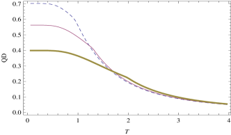
(b)

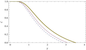
(c)

Figure 1: The QD (a), (c) and concurrence (b) versus T in the system with $z$-component parameter $D_{z}$. Here $J=1$. (a) Here $J_{z}=0.2$ and for the thick line $D_{z}=1.0$, normal line $D_{z}=0.7$, dashed line $D_{z}=0.5$. (b) Here $J_{z}=0.2$ and for the thick line $D_{z}=1.0$, normal line $D_{z}=0.7$, dashed line $D_{z}=0.5$. (c) Here $J_{z}=1$ and for the thick line $D_{z}=1.0$, normal line $D_{z}=0.7$, dashed line $D_{z}=0.5$.

Using the method in Ref. 1bennett96 ; wootters98 ; 2bennett96 , and results in li08 , we can also simply get the concurrence (In this paper, we use concurrence as the measure of entanglement) of this model at finite temperature. $C(\rho(T))=\frac{\beta J_{z}}{Z}(e^{2\beta w}-e^{-2\beta J_{z}}-e^{-2\beta w}-e^{-2\beta J_{z}})$ if $J_{z}>-w$, and $C(\rho(T))=0$ if $J_{z}<-w$.

Now by fixing some parameters we can see the variations of thermal QD and entanglement under the influence of other parameters. Looking at Fig. 1, where $J=1$, we can find that the QD decreases with increasing of temperature $T$. This tendency is similar to the situation of entanglement as shown in panel (b) where the conditions are the same. Differently, we can see from panel (b) that thermal entanglement will vanish when $T$ reaches certain point. And the larger parameter $D_{z}$ is the larger critical point is. The point denotes so-called critical temperature of the system. This behavior is caused by mixing of the maximally entanglement state with other states. In other words, it means that with the increasing of temperature $T$, thermal entanglement of the system will be disappeared at critical temperature and there is no entanglement resource to use then. However, as we see in panels (a) and (c), thermal QD will not reach zero point. It acts asymptotically near zero when the temperature is high. And in the temperature regions where thermal entanglement is zero while QD is still alive. We even find that we adjust $T$ very high (not shown in the plots), QD becomes very small but nonzero. This interesting phenomenon can be explained as follows. With the temperature grows, the role of thermal fluctuations exceeds quantum ones. However, it cannot kill the quantumness. As we know, entanglement is not the only part of quantum correlations. Based on Ollivier and Zurek’s argument zurek01 , it shows that absence of entanglement does not imply classcality. If you want to destroy the quantumness of a system, you should use the process of decoherence. Decoherence will eventually make the quantumness of a system to be zero and then the system will be in totally classical state. Since QD measures total quantum correlations, it is obvious that even temperature is high, without introducing the decoherence, quantum correlations will not vanish. So in this sense, QD is robust than entanglement at a finite temperature.

Focusing now at panel (a) of Fig. 1, when temperature $T$ increases, thermal fluctuation takes control of the system in this region, and the role of coupling constant such as $J$, $J_{z}$ and $D_{z}$ become weaker. So we can see the lines in panel (a) of Fig. 1 become concentrated together. Now we enhance the parameter $J_{z}$ to 1.0 as we can see in panel (c) of Fig. 1. We find that at the same temperature, lines become more separate than the case of panel (a). This effect is because of the influence of coupling constant $J_{z}$ makes the quantumness considerable. Next, let us take a look at panels (a) and (c) again and consider the influence of parameter $D_{z}$ to thermal QD. Due to the symmetry of DM interaction parameter, we can only take the strength of $D_{z}$ into account. So here only consider the $D_{z}>0$ case. Apparently, we can see a remarkable phenomenon (Also shown in Fig. 3) in certain region that when the parameter $D_{z}$ increases, thermal QD decreases while this trend of QD is in contrast to the behavior of entanglement. Since QD and entanglement are both kinds of measure of quantum correlations. This is very wired. Worth to be mentioned, this phenomenon appears in $D_{x}$ case as well, and we will analyze this in detail in Sec. IV.

Moreover, take a look at Fig. 2, where we fix $J=1$ and $D_{z}=1$. Asymptotical phenomenon of QD also appears at finite temperature for different $J_{z}$ in panel (a). However, we can see that QD increases with increasing of $J_{z}$. This is corresponding to the case of entanglement shown in panel (b). Here, $J_{z}$ as a anisotropic coupling constant of Heisenberg model, plays the same role in thermal QD as in the case of entanglement.

(a)

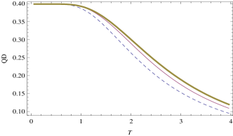
(b)

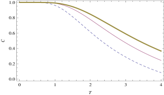
Figure 2: The QD (a) and concurrence (b) versus T in the system with $z$-component parameter $D_{z}$. Here $J=1$, $D_{z}=1$. (a) Here for the thick line $J_{z}=3.0$, normal line $J_{z}=2.0$ and dashed line $J_{z}=1.0$. (b) Here for the thick line $J_{z}=3.0$, normal line $J_{z}=2.0$ and dashed line $J_{z}=1.0$.

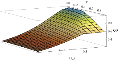
Figure 3: (Color online) The quantum discord is plotted versus $T$ and $D_{z}$ where $J=1$ and $J_{z}=0.2$.

III.2 XXZ Heisenberg model with DM interaction parameter $D_{x}$

Here we consider the case of the two-qubit anisotropic Heisenberg XXZ chain with DM interaction parameter $D_{x}$. The Hamiltonian $H^{\prime}$ of this model reads

$$H^{\prime}=J\sigma_{1}^{x}\sigma_{2}^{x}+J\sigma_{1}^{y}\sigma_{2}^{y}+J_{z}\sigma_{1}^{z}\sigma_{2}^{z}+D_{x}(\sigma_{1}^{y}\sigma_{2}^{z}-\sigma_{1}^{z}\sigma_{2}^{y}).$$ (14)

where $D_{x}$ is the $x$-component parameter of the DM interaction and other parameters are the same as in part A of this section.

Following the exact same approach in part A, we can get

$$H^{\prime}=\left(\begin{array}[]{cccc}J_{z}&iD_{x}&-iD_{x}&0\\ -iD_{x}&-J_{z}&2J&iD_{x}\\ iD_{x}&2J&-J_{z}&-iD_{x}\\ 0&-iD_{x}&iD_{x}&J_{z}\end{array}\right)$$ (15)

$$\rho^{\prime}(T)=\frac{1}{2Z^{\prime}}\left(\begin{array}[]{cccc}\mu_{+}&-\xi&\xi&\mu_{-}\\ \xi&\nu_{+}&\nu_{-}&-\xi\\ -\xi&\nu_{-}&\nu_{+}&\xi\\ \mu_{-}&\xi&-\xi&\mu_{+}\end{array}\right)$$ (16)

where $w^{\prime}=\sqrt{(J+J_{z})^{2}+4D_{x}^{2}}$ $\phi=\arctan(\frac{2D_{x}}{J+J_{z}-w^{\prime}})$ $\varphi=\arctan(\frac{2D_{x}}{J+J_{z}+w^{\prime}})$, and

$\mu_{\pm}=e^{-\beta J_{z}}\pm(e^{\beta(J-w^{\prime})}\sin^{2}{\phi}+e^{\beta(J+w^{\prime})}\sin^{2}{\varphi})$

$\nu_{\pm}=e^{\beta(J_{z}-2J)}\pm(e^{\beta(J-w^{\prime})}\cos^{2}{\phi}+e^{\beta(J+w^{\prime})}\cos^{2}{\varphi})$

$\xi=ie^{\beta(J-w^{\prime})}\sin{\phi}\cos{\phi}+ie^{\beta(J+w^{\prime})}\sin{\varphi}\cos{\varphi}$

$Z^{\prime}=2e^{-\beta J}\cosh[\beta(J-J_{z})]+2e^{\beta J}\cosh(\beta w^{\prime})$.

Also we can get $\rho^{\prime A}$ and $\rho^{\prime B}$ via straightforward calculation: $\rho^{\prime}_{A}=\rho^{\prime}_{B}=\frac{1}{2Z^{\prime}}(\mu_{+}+\nu_{+})I$ where $I$ is the identity operator.

Now, first we look at Fig. 4, where $J=1$ and $D_{x}=1$. We can see that when $J_{z}$ increases, the thermal QD becomes higher. This trend of QD is the same like entanglement case. (For better comparison we choose the exact the same value of parameters in Fig. 4 as in Ref. li08 ) And also, this fits with the behavior of $J_{z}$ in the system with $z$-component parameter $D_{z}$.

While looking at Fig. 5, we find that besides the asymptotical phenomenon mentioned above, we can also find the opposite trend of thermal QD and entanglement. So here we can derive that different DM parameters can both influence the behavior of QD and entanglement and make them move towards different directions in certain region. We will address this in Sec. IV.

In addition, back to the Fig. 1 and Fig. 5 which demonstrate the behaviors of thermal QD in aniosotropic Heisenberg model with parameters $D_{z}$ and $D_{x}$. It is obvious there are some differences between two different cases. First, let us look at panel (a) of Fig. 1 and panel (b) of Fig. 5, we find that in the situation where other parameters are exactly the same, $D_{x}$ is more reliable than $D_{z}$ when T becomes higher. This indicates that $D_{z}$ is easy to influence by the increasing of $T$ (This also shown in Fig. 3 and Fig. 6). And from Fig. 1 and Fig. 5 we can find that if we tune the parameter $J_{z}$ larger, thermal QD depending on different $D_{x}$ change more obviously than the case of parameter $D_{z}$. This means that parameter $D_{x}$ is more sensitive in certain condition along with change of parameters such as $J_{z}$. So we can derive from this results that it is more efficient to use parameter $D_{x}$ to control the QD. In addition, we can also find that when tune parameter $J_{z}$ to 1.0, the two plots (panel (c) of Fig. 1 and panel (a) of Fig. 5) become similar, which is mainly because the DM interactions now are not the dominating parameters controlling the behavior of the system.

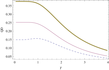
Figure 4: The QD versus T in the system with $x$-component parameter $D_{x}$. Here $J=1$, $D_{x}=1$ and for the thick line $J_{z}=0.9$, normal line $J_{z}=0.4$, dashed line $J_{z}=0$.

(a)

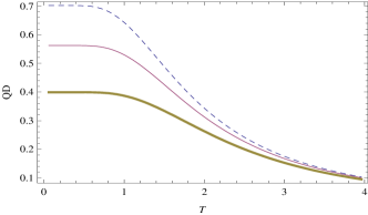
(b)

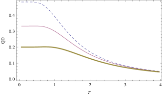
Figure 5: The QD versus T in the system with $x$-component parameter $D_{x}$. Here $J=1$. (a) Here $J_{z}=1.0$ and for the thick line $D_{z}=1.0$, normal line $D_{z}=0.7$, dashed line $D_{z}=0.5$. (b) Here $J_{z}=0.2$ and for the thick line $D_{z}=1.0$, normal line $D_{z}=0.7$, dashed line $D_{z}=0.5$.

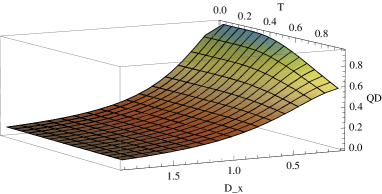
Figure 6: (Color online) The quantum discord is plotted versus $T$ and $D_{x}$ where $J=1$ and $J_{z}=0.2$.

IV Discussion about opposite tendency of thermal QD and entanglement

In this section, we will discuss the opposite tendency of thermal QD and entanglement appeared in Sec. III.

In previous section, we find that, in certain regions, when parameter $D_{z}$ increases, thermal QD decreases while at the same time thermal entanglement increases. This also appears in the case of parameter $D_{x}$. So we say that when we tune the parameters of DM interaction, entanglement and QD have the opposite trend of movement. Obviously, this notable phenomenon is very wired since both QD and entanglement quantify the quantumness of correlations. There are some underlying reasons about that. Although QD and entanglement both kinds of measure of quantum correlations. Entanglement is a non-local correlation while QD figures a measure of whole quantumness of correlations for a pairwise system. There are some other quantum correlations without entanglement which can be characterized by QD but not any kinds of entanglement measure such as concurrence. And we reveal that these other quantum correlations have remarkably different characteristic from the entanglement. Recent researches dat08 ; lanyon08 ; kni98 also suggest that these other quantum correlations can also be an important resource and maybe take respondence in mixed state quantum computation. Secondly, DM interaction is a magnetic term arising from the spin-orbit coupling. The staggered DM interactions bring on helical magnetic structures due to its form $\mathbf{D}\cdot[\mathbf{S_{1}}\times\mathbf{S_{2}}]$, where $\mathbf{S_{1}}$, $\mathbf{S_{2}}$ denote the spins and $\mathbf{D}$ is DM vector. DM interaction can contribute the strong planar quantum fluctuations which pose the alignment ordering to both qubit-1 and qubit-2 in two-qubit system. Some researches jafari08 ; kargarian09 have shown that in certain condition, DM interaction can build entanglement. So it is acceptable that entanglement increase with increasing of DM interaction in this paper.

Now we can see that since QD figures the whole quantum correlations including entanglement, the phenomenon here indicate that, the other quantum correlations without entanglement we mentioned above decrease rapidly (more rapidly than the increase of entanglement at the same time) with increasing of parameters of DM interaction. So we can see from Fig. 1 and Fig. 5. that when QD decreases while the entanglement increases with the increasing of DM interactions. Here, this phenomenon can coincide what we have raised above that the characteristic of QD is exotic. Furthermore, using this characteristic, under certain conditions, we can tune the parameters of DM interactions to increase the entanglement of a system and meanwhile decrease the other quantum correlations of the same system. The advantage of the method is obvious. If you want to take entanglement as a quantum resource to do quantum tasks, you want to enhance your entanglement resource and make the other quantum correlations of system as less as possible, this approach would offer a possible solution.

V Conclusion

The thermal QD of a two-qubit anisotropic Heisenberg XXZ chain with two distinct DM interaction parameters is investigated. We find that thermal QD is more robust than thermal entanglement versus temperature $T$. And numerical results indicate that it is more efficient to control QD in the model with parameter $D_{x}$ than with parameter $D_{z}$. Furthermore, with the increasing of parameters $D_{z}$ and $D_{x}$, thermal QD varies oppositely to the case of entanglement. This phenomenon reveals that quantum correlations without entanglement have quite exotic characteristic from entanglement. In addition, this effect also offers a solution to make the entanglement of a system enhanced.

- (1) R. Horodecki, et al. Rev. Mod. Phys. 81, 865 (2009).
- (2) M. A. Nielson and I. L. Chuang, Quantum Computation and Quantum Information (Cambridge University Press, Cambridge, England, 2000).
- (3) C. H. Bennett, et al. Phys. Rev. Lett. 70, 1895 (1993).
- (4) D. Bouwmeester, et al. Nature. 390, 575 (1997).
- (5) C. H. Bennett, and S. J. Wiesner, Phys. Rev. Lett. 69, 2881 (1992).
- (6) P. W. Shor, SIAMJ. Comp., 26, 1484 (1997).
- (7) L. K. Grover, Phys. Rev. Lett. 79, 325 (1997).
- (8) J. Maziero, et al. Phys. Rev. A 80, 044102 (2009).
- (9) H. Ollivier and W. H. Zurek, Phys. Rev. Lett. 88, 017901 (2001).
- (10) M. S. Sarandy, Phys. Rev. A. 80, 022108 (2009).
- (11) R. Dillenschneider, Phys. Rev. B 78, 224413 (2008).
- (12) S. Luo, Phys. Rev. A 77, 042303 (2008).
- (13) T. Werlang, et al. Phys. Rev. A 80, 024103 (2009).
- (14) T. Werlang and G. Rigolin, e-pring arXiv:quant-ph/0911.3903.
- (15) Yi-Xin. Chen and Sheng-Wen. Li, e-pring arXiv:quant-ph/0912.3874.
- (16) A. Datta, et al. Phys. Rev. Lett. 100, 050502 (2008).
- (17) B. P. Lanyon, et al. Phys. Rev. Lett. 101, 200501 (2008).
- (18) E. Knill, and R. Laflamme, Phys. Rev. Lett. 81, 5672 (1998).
- (19) B. Trauzettel, et al. Nat. Phys. 3, 192 (2007).
- (20) R. Hanson, et al. Rev. Mod. Phys. 79, 1217 (2007).
- (21) L. F. Wei, Yu-xi Liu, and Franco. Nori, Phys. Rev. Lett. 96, 246803 (2006).
- (22) D. Porras and J. I. Cirac Phys. Rev. Lett. 92, 207901 (2004).
- (23) Shi-Biao Zheng and Guang-Can Guo, Phys. Rev. Lett. 85, 2392 (2000).
- (24) X. G. Wang, Phys. Rev. A 66, 044305 (2002).
- (25) Y. Sun, et al. Phys. Rev. A 68, 044301 (2003).
- (26) G. F. Zhang and S. S. Li, Phys. Rev. A 72, 034302 (2005).
- (27) M. C. Arnesen, et al. Phys. Rev. Lett. 87, 017901 (2001).
- (28) M. Asoudeh and V. Karimipour Phys. Rev. A 71, 022308 (2005).
- (29) D. Gunlycke, et al. Phys. Rev. A 64, 042302 (2001).
- (30) I. Dzyaloshinsky, J. Phys. Chem. Solids 4, 241 (1958).
- (31) T. Moriya, Phys. Rev. 120, 91 (1960).
- (32) D. N. Aristov and S. V. Maleyev, Phys. Rev. B 62, 751 (2000).
- (33) M. Kargarian, et al. Phys. Rev. A 79, 042319 (2009).
- (34) R. Jafari, et al. Phys. Rev. B 78, 214414 (2008).
- (35) Da-Chuang Li, Xian-Ping Wang and Zhuo-Liang Cao, J. Phys.: Condens. Matter. 20, 325229 (2008).
- (36) C. H. Bennett, et al. Phys. Rev. A 54, 3824 (1996).
- (37) W. K. Wootters, Phys. Rev. Lett. 80, 2245 (1998).
- (38) C. H. Bennett, et al. Phys. Rev. A 53, 2046 (1996).
- (39) L. Henderson and V. Vedral, J. Phys. A 34, 6899 (2001).
- (40) V. Verdral, Rev. Mod. Phys. 74, 197 (2002).
- (41) B. Groisman, et al. Phys. Rev. A. 72, 032317 (2005).
- (42) M. A. Nielsen, e-pring arXiv:quant-ph/0011036.