BS$\Delta$Es and BSDEs with non-Lipschitz drivers: Comparison, convergence and robustness

Abstract

We provide existence results and comparison principles for solutions of backward stochastic difference equations (BS$\Delta$Es) and then prove convergence of these to solutions of backward stochastic differential equations (BSDEs) when the mesh size of the time-discretizaton goes to zero. The BS$\Delta$Es and BSDEs are governed by drivers $f^{N}(t,\omega,y,z)$ and $f(t,\omega,y,z),$ respectively. The new feature of this paper is that they may be non-Lipschitz in $z$. For the convergence results it is assumed that the BS$\Delta$Es are based on $d$-dimensional random walks $W^{N}$ approximating the $d$-dimensional Brownian motion $W$ underlying the BSDE and that $f^{N}$ converges to $f$. Conditions are given under which for any bounded terminal condition $\xi$ for the BSDE, there exist bounded terminal conditions $\xi^{N}$ for the sequence of BS$\Delta$Es converging to $\xi$, such that the corresponding solutions converge to the solution of the limiting BSDE. An important special case is when $f^{N}$ and $f$ are convex in $z.$ We show that in this situation, the solutions of the BS$\Delta$Es converge to the solution of the BSDE for every uniformly bounded sequence $\xi^{N}$ converging to $\xi$. As a consequence, one obtains that the BSDE is robust in the sense that if $(W^{N},\xi^{N})$ is close to $(W,\xi)$ in distribution, then the solution of the $N$th BS$\Delta$E is close to the solution of the BSDE in distribution too.

and

1 Introduction

The aim of this paper is to obtain general convergence results of solutions of stochastic backward equations in discrete time (BS$\Delta$Es) to solutions of stochastic backward equations in continuous time (BSDEs). The discrete equations are governed by drivers $f^{N}(t,\omega,y,z)$, $N\in\mathbb{N}$, and the continuous one by $f(t,\omega,y,z)$. The new feature of this paper is that $f^{N}$ and $f$ may be non-Lipschitz in $z$. We assume that the BS$\Delta$Es are based on $d$-dimensional random walks $W^{N}$ converging to the $d$-dimensional Brownian motion $W$ underlying the BSDE and that $f^{N}$ tends to $f$. Convergence results for Lipschitz drivers have been obtained by Briand et al. [4, 5] as well as Toldo [28, 29]. In these papers, existence and uniqueness of solutions follow from a Picard iteration argument. Using results on convergence of filtrations from Coquet et al. [12], it can be shown that the Picard sequences approach each other asymptotically, which yields general convergence results. In the case of non-Lipschitz drivers this approach does not work, and neither the existence of solutions of BS$\Delta$Es nor their convergence to their counterparts in continuous time are clear.

In this paper, we start with a careful analysis of BS$\Delta$Es. Central to our approach is Theorem 4.2 which provides a comparison principle for BS$\Delta$Es. It requires drivers that can grow faster than linearly but strictly less than quadratically in $z$. Kobylanski [21] showed existence, comparison and uniqueness of solutions to BSDEs with general bounded terminal conditions and drivers of quadratic growth in $z$. However, in discrete time the situation is different. Example 4.1 shows that neither a general comparison principle nor convergence of solutions for diminishing step sizes can hold for BS$\Delta$Es if the drivers grow quadratically in $z$. Our main convergence results are Theorems 5.9 and 6.2. Theorem 5.9 shows that if $f^{N}$ and $f$ grow less than quadratically in $z$, then for any bounded terminal condition $\xi$ for the BSDE, there exist bounded terminal conditions $\xi^{N}$ for the BS$\Delta$Es such that the corresponding solutions $Y^{N}$ converge to the solution $Y$ of the BSDE in the following sense:

$$\sup_{0\leq t\leq T}\bigl{|}Y^{N}_{t}-Y_{t}\bigr{|}\to 0\qquad\mbox{in }L^{2}\mbox{ when }N\to\infty.$$ (1)

Furthermore, if $\xi$ is of the form $\xi=\varphi(W_{s_{1}},\ldots,W_{s_{n}})$ for a bounded, uniformly continuous function $\varphi$, then the $\xi^{N}$ can be chosen as $\xi^{N}=\varphi(W^{N}_{s_{1}},\ldots,W^{N}_{s_{n}})$. In Theorem 6.2, we prove that if the drivers $f^{N}$ are convex in $z$, then (1) holds for every sequence of uniformly bounded $\xi^{N}$ converging to $\xi$ in $L^{2}$. As a corollary one obtains that if $(W^{N},\xi^{N})$ is close to $(W,\xi)$ in distribution, then $Y^{N}$ is close to $Y$ in distribution too.

Discrete schemes for the approximation of solutions of BSDEs have been studied by a number of authors; see for instance, Ma et al. [23], Douglas et al. [15], Bally [1], Chevance [9], Coquet et al. [11], Ma et al. [22], Zhang and Zheng [31], Zhang [30], Bouchard and Touzi [3], Gobet et al. [18] and Otmani [17]. However, in all these papers the drivers are assumed to be Lipschitz. Recently, Imkeller and Reis [20] as well as Richou [27] have obtained results on the convergence of solutions of discretized BSDEs with drivers of quadratic growth under regularity assumptions on the terminal conditions and for specially chosen discrete-time drivers $f^{N}$. In Cheridito and Stadje [8] convergence results are shown for convex drivers and terminal conditions that are Lipschitz continuous in the underlying Brownian motion. Our results hold for general terminal conditions and general drivers $f^{N}$ converging to $f$. But they need subquadratic growth of $f^{N}$ in $z$. Comparison results for BS$\Delta$Es have also been studied in Cohen and Elliott [10] but under different assumptions than here.

The structure of the paper is as follows: In Section 2, we introduce the notation and provide some background material. Then we give an example showing that BS$\Delta$Es with non-Lipschitz drivers need not converge if the terminal conditions are not uniformly bounded. In Section 3, we show that BS$\Delta$Es admit solutions under very mild assumptions if the time-discretization is fine enough. Section 4 starts with an example showing two facts about BS$\Delta$Es with drivers of quadratic growth: (a) a general comparison principle cannot hold and (b) solutions of BS$\Delta$Es can explode if the step-size goes to zero even if the terminal conditions are uniformly bounded and converge to zero in $L^{2}$. We then prove a general comparison principle for subquadratic BS$\Delta$Es. Section 5 gives convergence results of solutions of general BS$\Delta$Es to solutions of BSDEs, and in Section 6 we prove convergence results for drivers that are convex in $z$.

2 Notation and setup

We fix a finite time horizon $T\in\mathbb{R}_{+}$. As underlying process for the BSDE, we take a $d$-dimensional Brownian motion $(W_{t})_{t\in[0,T]}$ on a probability space $(\Omega,\mathcal{F},\mathbb{P})$ and denote by $(\mathcal{F}_{t})_{t\in[0,T]}$ the augmented filtration generated by $(W_{t})_{t\in[0,T]}$. Equalities and inequalities between random variables will, as usual, be understood in the $\mathbb{P}$-almost sure sense. As approximating processes we consider a sequence $(W^{N}_{t})_{t\in[0,T]}$, $N\in\mathbb{N}$, of $d$-dimensional square-integrable martingales on $(\Omega,\mathcal{F},\mathbb{P})$ starting at $0$ with independent increments satisfying the following three conditions:

1. [(C2)]

2. For every $N$ there exists a finite sequence $0=t_{0}^{N}<t^{N}_{1}<\cdots<t^{N}_{i_{N}}=T$ such that

   $$\lim_{N\rightarrow\infty}\sup_{i}\bigl{|}t^{N}_{i+1}-t^{N}_{i}\bigr{|}=0$$

   and $W^{N}_{t}$ is constant on each of the intervals $[t^{N}_{i},t^{N}_{i+1}).$

3. $$\Delta\bigl{\langle}W^{N,k}\bigr{\rangle}_{t^{N}_{i}}=\Delta\bigl{\langle}W^{N,l}\bigr{\rangle}_{t^{N}_{i}}>0\qquad\mbox{for all }i\mbox{ and }1\leq k,l\leq d.$$

4. $$\lim_{N\to\infty}{\mathbb{E}}\Bigl{[}\sup_{0\leq t\leq T}\bigl{|}W^{N}_{t}-W_{t}\bigr{|}^{2}\Bigr{]}=0,$$

   where $|\cdot|$ denotes the standard Euclidean norm on $\mathbb{R}^{d}\colon\ |x|:=(\sum_{i=1}^{d}x_{i}^{2})^{1/2}$.

Let $(\mathcal{F}^{N}_{t})$ be the filtration generated by $(W^{N}_{t})$ and define $\langle W^{N}\rangle_{t}:=\langle W^{N,k}\rangle_{t}$. Since $W^{N}$ has independent increments, $\langle W^{N}\rangle_{t}=\langle W^{N,k}\rangle_{t}$ is equal to ${\mathbb{E}}[(W^{N,k}_{t})^{2}]$, and it follows from (C3) that

$$\sup_{0\leq t\leq T}\bigl{|}\bigl{\langle}W^{N}\bigr{\rangle}_{t}-t\bigr{|}=\sup_{0\leq t\leq T}\bigl{|}{\mathbb{E}}\bigl{[}\bigl{(}W^{N,k}_{t}\bigr{)}^{2}-\bigl{(}W^{k}_{t}\bigr{)}^{2}\bigr{]}\bigr{|}\to 0\qquad\mbox{for }N\to\infty.$$ (2)

In particular,

$$\lim_{N\rightarrow\infty}\max_{i}\bigl{|}\Delta\bigl{\langle}W^{N}\bigr{\rangle}_{t^{N}_{i}}\bigr{|}=0.$$

Our standard example for the approximating processes $W^{N}$ will be $d$-dimensional Bernoulli random walks.

Example 2.1.

Let

$$t^{N}_{i}=i\frac{T}{N}\quad\mbox{and}\quad\tilde{W}^{N,k}_{t^{N}_{i}}=\sqrt{\frac{T}{N}}\sum_{j=1}^{i}X^{N,k}_{j}$$

for i.i.d. random variables $X^{N,k}_{j}$ on a probability space $(\tilde{\Omega},\tilde{\mathcal{F}},\tilde{\mathbb{P}})$ with distribution $\tilde{\mathbb{P}}[X^{N,k}_{j}=\pm 1]=1/2$. Extend $(\tilde{W}^{N}_{t})$ to $[0,T]$ such that it is constant on the intervals $[t^{N}_{i},t^{N}_{i+1})$. Then conditions (C1) and (C2) are satisfied. To fulfill (C3), one must transfer the random walks to another probability space. Since they converge to $d$-dimensional Brownian motion in distribution, there exists a probability space $(\Omega,\mathcal{F},\mathbb{P})$ with a $d$-dimensional Brownian motion $(W_{t})$ and random walks $(W^{N}_{t})$ having the same distributions as $(\tilde{W}^{N}_{t})$ such that

$$\sup_{0\leq t\leq T}\bigl{|}W^{N}_{t}-W_{t}\bigr{|}\to 0\quad\mbox{almost surely}\quad\mbox{as }N\to\infty;$$ (3)

see, for instance, Theorem I.2.7 in Ikeda and Watanabe [19]. It can be shown that the sequence $\sup_{0\leq t\leq T}|W^{N}_{t}-W_{t}|^{2}$ is uniformly integrable. Therefore, the convergence (3) also holds in $L^{2}$, and condition (C3) is satisfied.

The driver of the BSDE is a $\mathcal{P}\otimes\mathcal{B}(\mathbb{R})\otimes\mathcal{B}(\mathbb{R}^{d})$-measurable function

$$f\mathchoice{\nobreak\,\colon}{\nobreak\,\colon}{\nobreak\,\colon\;}{\nobreak\,\colon\;}[0,T]\times\Omega\times\mathbb{R}\times\mathbb{R}^{d}\rightarrow\mathbb{R},$$

where $\mathcal{P}$ denotes the predictable $\sigma$-algebra on $[0,T]\times\Omega$ with respect to $(\mathcal{F}_{t})$ and $\mathcal{B}(\mathbb{R})$ and $\mathcal{B}(\mathbb{R}^{d})$ are the Borel $\sigma$-algebras on $\mathbb{R}$ and $\mathbb{R}^{d}$, respectively. We will assume throughout the paper that for fixed $(t,\omega)$, $f(t,\omega,y,z)$ is continuous in $(y,z)$. Then $\mathcal{P}\otimes\mathcal{B}(\mathbb{R})\otimes\mathcal{B}(\mathbb{R}^{d})$-measurability of $f$ is equivalent to $(t,\omega)\mapsto f(t,\omega,y,z)$ being predictable for all fixed $(y,z)$.

The approximating BS$\Delta$Es have drivers

$$f^{N}\mathchoice{\nobreak\,\colon}{\nobreak\,\colon}{\nobreak\,\colon\;}{\nobreak\,\colon\;}[0,T]\times\Omega\times\mathbb{R}\times\mathbb{R}^{d}\rightarrow\mathbb{R}$$

that are continuous in $(y,z)$, constant on the intervals $(t^{N}_{i},t^{N}_{i+1}]$ and such that $\omega\mapsto f^{N}(t^{N}_{i+1},\omega,y,z)$ is $\mathcal{F}^{N}_{t^{N}_{i}}$-measurable. As usual, we henceforth suppress the dependence of $f$ and $f^{N}$ on $\omega$ in the notation.

The terminal conditions for the BSDE and BS$\Delta$Es are given by random variables $\xi$, $\xi^{N}$ that are measurable with respect to $\mathcal{F}_{T}$ and $\mathcal{F}^{N}_{T}$, respectively.

A solution of the BSDE consists of a pair of predictable processes $(Y_{t},Z_{t})$ with values in $\mathbb{R}\times\mathbb{R}^{d}$ such that

$${\mathbb{E}}\Bigl{[}\sup_{0\leq t\leq T}Y_{t}^{2}\Bigr{]}<\infty,\qquad{\mathbb{E}}\biggl{[}\biggl{(}\int_{0}^{T}|Z_{s}|^{2}\,\mathrm{d}s\biggr{)}^{1/2}\biggr{]}<\infty,$$

and

$$Y_{t}=\xi+\int_{t}^{T}f(s,Y_{s},Z_{s})\,\mathrm{d}s-\int_{t}^{T}Z_{s}\,\mathrm{d}W_{s},\qquad 0\leq t\leq T.$$ (4)

In contrast to $(W_{t})$, the approximating processes $(W^{N}_{t})$ do in general not have the predictable representation property. Therefore, a solution of the $N$th BS$\Delta$E is a triple of $(\mathcal{F}^{N}_{t})$-adapted processes $(Y^{N}_{t},Z^{N}_{t},M^{N}_{t})$ taking values in $\mathbb{R}\times\mathbb{R}^{d}\times\mathbb{R}$ such that $(Y^{N}_{t})$ is constant on the intervals $[t^{N}_{i},t^{N}_{i+1})$, $(Z^{N}_{t})$ is constant on the intervals $(t^{N}_{i},t^{N}_{i+1}]$, $(M^{N}_{t})$ is a square-integrable martingale starting at $0$ and orthogonal to $(W^{N}_{t})$ that is constant on the intervals $[t^{N}_{i},t^{N}_{i+1})$ and

$$Y^{N}_{t}=\xi^{N}+\int_{(t,T]}f^{N}\bigl{(}s,Y^{N}_{s-},Z^{N}_{s}\bigr{)}\,\mathrm{d}\bigl{\langle}W^{N}\bigr{\rangle}_{s}-\int_{(t,T]}Z^{N}_{s}\,\mathrm{d}W^{N}_{s}-\bigl{(}M^{N}_{T}-M^{N}_{t}\bigr{)}.$$ (5)

Due to the particular form of $(Y^{N}_{t},Z^{N}_{t},M^{N}_{t})$, (5) is equivalent to

$$Y^{N}_{t^{N}_{i}} = Y^{N}_{t^{N}_{i+1}}+f^{N}\bigl{(}t^{N}_{i+1},Y^{N}_{t^{N}_{i}},Z^{N}_{t^{N}_{i+1}}\bigr{)}\Delta\bigl{\langle}W^{N}\bigr{\rangle}_{t^{N}_{i+1}}-Z^{N}_{t^{N}_{i+1}}\Delta W^{N}_{t^{N}_{i+1}}-\Delta M^{N}_{t^{N}_{i+1}},$$ (6)

$$Y^{N}_{T} = \xi^{N}.$$ (7)

Note that if $(W^{N}_{t})$ is a one-dimensional Bernoulli random walk, it has the predictable representation property and the orthogonal martingale terms in (5) and (6) disappear.

It is well known that if the driver $f$ is Lipschitz-continuous in $(y,z)$ and the terminal condition $\xi$ is in $L^{2}$, the BSDE (4) admits a unique solution $(Y,Z)$; see, for instance, Pardoux and Peng [25] or the survey paper by El Karoui et al. [16]. Concerning the approximation of BSDEs with Lipschitz drivers, we recall the following result from Briand et al. [5]. Their assumptions are slightly different. But the result also holds in our setup.

Theorem 2.2 ((Briand et al. [5]))

Assume $\xi^{N}\to\xi$ in $L^{2}$ and there exists a constant $K\in\mathbb{R}_{+}$ such that for all $N\in\mathbb{N}$, $y,y^{\prime}\in\mathbb{R}$ and $z,z^{\prime}\in\mathbb{R}^{d}$ the following four conditions hold:

1. [(iii)]

2. ${\mathbb{E}}[\sup_{t}f(t,0,0)^{2}]<\infty$;

3. $|f(t,y,z)-f(t,y^{\prime},z^{\prime})|\leq K(|y-y^{\prime}|+|z-z^{\prime}|)$;

4. $|f^{N}(t,y,z)-f^{N}(t,y^{\prime},z^{\prime})|\leq K(|y-y^{\prime}|+|z-z^{\prime}|)$;

5. $\sup_{t}|f^{N}(t,y,z)-f(t,y,z)|\rightarrow 0\mbox{ in }L^{2}\mbox{ as }N\to\infty$.

Then, for $N$ large enough, the $N$th BSDE has a unique solution $(Y^{N},Z^{N},M^{N})$, and

$$\sup_{t}\biggl{(}\bigl{|}Y^{N}_{t}-Y_{t}\bigr{|}+\biggl{|}\int_{0}^{t}Z^{N}_{s}\,\mathrm{d}W^{N}_{s}-\int_{0}^{t}Z_{s}\,\mathrm{d}W_{s}\biggr{|}+\bigl{|}M^{N}_{t}\bigr{|}\biggr{)}\stackrel{{\scriptstyle(N\rightarrow\infty)}}{{\to}}0\qquad\mbox{in }L^{2}$$

as well as

$$\sup_{t}\Biggl{(}\sum_{k=1}^{d}\biggl{|}\int_{0}^{t}Z^{N,k}_{s}\,\mathrm{d}\bigl{\langle}W^{N}\bigr{\rangle}_{s}-\int_{0}^{t}Z^{k}_{s}\,\mathrm{d}s\biggr{|}^{2}+\biggl{|}\int_{0}^{t}\bigl{|}Z^{N}_{s}\bigr{|}^{2}\,\mathrm{d}\bigl{\langle}W^{N}\bigr{\rangle}_{s}-\int_{0}^{t}|Z_{s}|^{2}\,\mathrm{d}s\biggr{|}\Biggr{)}$$

$$\quad\stackrel{{\scriptstyle(N\rightarrow\infty)}}{{\to}}0\qquad\mbox{in }L^{1},$$

where $(Y,Z)$ is the unique solution of the BSDE (4).

Remark 2.3.

Two special cases of terminal conditions satisfying $\xi^{N}\to\xi$ in $L^{2}$ are:

1. [(b)]

2. $\xi=\varphi(W_{T})$ and $\xi^{N}=\varphi(W^{N}_{T})$ for a continuous function $\varphi\mathchoice{\nobreak\,\colon}{\nobreak\,\colon}{\nobreak\,\colon\;}{\nobreak\,\colon\;}\mathbb{R}^{d}\to\mathbb{R}$ such that $\varphi^{2}(W^{N}_{T})$, $N\in\mathbb{N}$, is uniformly integrable.

3. $\xi\in L^{2}(\mathcal{F}_{T})$ general and $\xi^{N}={\mathbb{E}}[\xi|\mathcal{F}^{N}_{T}]$.

The aim of this paper is to obtain similar convergence results for non-Lipschitz drivers. However, the following example shows that we cannot hope for general results under the sole assumption $\xi^{N}\to\xi$ in $L^{2}$.

Example 2.4.

Consider a one-dimensional Bernoulli random walk with $T=1$, $t_{i}^{N}=i/N$ and $\mathbb{P}[\Delta W^{N}_{t^{N}_{i}}=\pm\sqrt{1/N}]=1/2$. Then

$$\Delta\bigl{\langle}W^{N}\bigr{\rangle}_{t_{i}^{N}}={\mathbb{E}}\bigl{[}\bigl{(}\Delta W^{N}_{t^{N}_{i}}\bigr{)}^{2}\bigr{]}=1/N.$$

Fix $q\in(1,2)$ and a sequence of constants $a^{N}\geq 2N^{({1-q/2})/({q-1})}$. Consider the BS$\Delta$Es

$$Y^{N}_{t_{i}^{N}}=Y^{N}_{t_{i+1}^{N}}+\bigl{|}Z_{t^{N}_{i+1}}^{N}\bigr{|}^{q}\Delta\bigl{\langle}W^{N}\bigr{\rangle}_{t^{N}_{i+1}}-Z^{N}_{t^{N}_{i+1}}\Delta W^{N}_{t^{N}_{i+1}},\qquad Y^{N}_{T}=a^{N}1_{\{W^{N}_{t_{N}}=\sqrt{N}\}}.$$

It can easily be checked that

$$Z^{N}_{t^{N}_{N}}=\frac{\sqrt{N}}{2}a^{N}1_{\{W^{N}_{t_{N-1}^{N}}=({N-1})/{\sqrt{N}}\}}\quad\mbox{and}\quad Y^{N}_{t_{N-1}^{N}}=a^{N}_{t_{N-1}^{N}}1_{\{W^{N}_{t_{N-1}^{N}}=({N-1})/{\sqrt{N}}\}}$$

for

$$a^{N}_{t_{N-1}^{N}}=\frac{a^{N}}{2}+2^{-q}N^{q/2-1}\bigl{(}a^{N}\bigr{)}^{q}\geq a^{N}.$$

Continuing this way one gets

$$Z^{N}_{t^{N}_{N-1}}=\frac{\sqrt{N}}{2}a^{N}_{t^{N}_{N-1}}1_{\{W^{N}_{t_{N-2}^{N}}=({N-2})/{\sqrt{N}}\}}\quad\mbox{and}\quad Y^{N}_{t_{N-2}^{N}}=a^{N}_{t_{N-2}^{N}}1_{\{W^{N}_{t_{N-2}^{N}}=({N-2})/{\sqrt{N}}\}}$$

with

$$a^{N}_{t_{N-2}^{N}}=\frac{a^{N}_{t_{N-1}}}{2}+2^{-q}N^{q/2-1}\bigl{(}a^{N}_{t_{N-1}^{N}}\bigr{)}^{q}\geq a^{N}_{t_{N-1}^{N}},$$

and so on. In particular,

$$Y^{N}_{0}\geq a^{N}\geq 2N^{({1-(q/2)})/({q-1})}\to\infty\qquad\mbox{for }N\to\infty.$$

Note that for $a^{N}=2N^{({1-q/2})/({q-1})}$, one has $\xi^{N}\to 0$ in $L^{p}$ for all $p\in(0,\infty)$ but not in $L^{\infty}$.

The example shows that in the case of super-linear growth of $f^{N}$ in $z$ one cannot expect convergence of the discrete-time solutions if the terminal conditions are uniformly $L^{p}$-bounded and converge in $L^{p}$ for $p<\infty$. This is not unexpected since in the literature on BSDEs with non-Lipschitz drivers it is usually required that the terminal condition be in $L^{\infty}$ or sufficiently well exponentially integrable (see Kobylanski [21], or Briand and Hu [6]). Consequently, in this paper, we will always assume:

1. [(C4)]

2. $$\sup_{N}\bigl{\|}\xi^{N}\bigr{\|}_{\infty}<\infty\quad\mbox{and}\quad\|\xi\|_{\infty}<\infty.$$

We shortly summarize the notation and assumptions that have been introduced in this section:

• $W^{N}$, $N\in\mathbb{N}$, is a sequence of discrete-time martingales approximating the $d$-dimensional Brownian motion $W$.

• $f$ and $\xi$ are the driver and terminal condition of the BSDE (4). A solution to (4) will be denoted by $(Y,Z)$.

• $f^{N}$ and $\xi^{N}$ are the drivers and terminal conditions of the BS$\Delta$Es (5). Solutions will be denoted by $(Y^{N},Z^{N},M^{N})$.

• We always assume (C1)–(C4).

3 Solutions of BS$\Delta$Es

In this section, we present two results on solutions of BS$\Delta$Es that will be needed later in the paper. Their proofs are straightforward and therefore, given in the Appendix.

Lemma 3.1.

If a solution $(Y^{N},Z^{N},M^{N})$ of the $N$th BS$\Delta$E exists, one has

$$Y^{N}_{t^{N}_{i}}-f^{N}\bigl{(}t^{N}_{i+1},Y^{N}_{t^{N}_{i}},Z^{N}_{t^{N}_{i+1}}\bigr{)}\Delta\bigl{\langle}W^{N}\bigr{\rangle}_{t^{N}_{i+1}}={\mathbb{E}}\bigl{[}Y^{N}_{t^{N}_{i+1}}|\mathcal{F}^{N}_{t^{N}_{i}}\bigr{]},$$ (8)

and the pair $(Z^{N},M^{N})$ is uniquely determined by $Y^{N}$ through

$$Z^{N,k}_{t^{N}_{i+1}} = \frac{{\mathbb{E}}[Y^{N}_{t^{N}_{i+1}}\Delta W^{N,k}_{t^{N}_{i+1}}|\mathcal{F}^{N}_{t^{N}_{i}}]}{\Delta\langle W^{N}\rangle_{t^{N}_{i+1}}},$$ (9)

$$\Delta M^{N}_{t^{N}_{i+1}} = Y^{N}_{t^{N}_{i+1}}-{\mathbb{E}}\bigl{[}Y^{N}_{t^{N}_{i+1}}|\mathcal{F}^{N}_{t^{N}_{i}}\bigr{]}-Z^{N}_{t^{N}_{i+1}}\Delta W^{N}_{t^{N}_{i+1}}.$$ (10)

Concerning the existence of solutions to BS$\Delta$Es, one has the following result. For the special case where $W^{N}$ is a one-dimensional Bernoulli random walk, see Peng [26].

Proposition 3.2.

Assume there exists a constant $K\in\mathbb{R}_{+}$ and a locally bounded function $g\mathchoice{\nobreak\,\colon}{\nobreak\,\colon}{\nobreak\,\colon\;}{\nobreak\,\colon\;}\mathbb{R}^{d}\to\mathbb{R}_{+}$ such that

$$\bigl{|}f^{N}(t,y,z)\bigr{|}\leq K\bigl{(}1+|y|+g(z)\bigr{)}\quad\mbox{and}\quad\max_{i}\Delta\bigl{\langle}W^{N}\bigr{\rangle}_{t^{N}_{i}}<1/K.$$

Then the $N$th BS$\Delta$E has a solution $(Y^{N},Z^{N},M^{N})$ such that $Y^{N}$ and $Z^{N}$ are bounded. If $W^{N}$ is bounded, then so is $M^{N}$.

Remark 3.3.

For $\max_{i}\Delta\langle W^{N}\rangle_{t^{N}_{i}}\geq 1/K$ a solution of the $N$th BS$\Delta$E might not exist. For example, let $W^{1}$ be a one-dimensional Bernoulli random walk with $t_{0}^{1}=0$, $t_{1}^{1}=1=T$, $\mathbb{P}[\Delta W^{1}_{1}=\pm 1]=1/2$, $\xi^{1}=1$ and $f^{1}(t,y,z)=y$. Since the terminal condition is deterministic, one must choose $Z^{1}_{1}=0$, and (2) becomes

$$Y^{1}_{0}-Y^{1}_{0}=1,$$

an equation without solution.

4 Comparison principle for BS$\Delta$Es

Our main tool to derive convergence results will be a comparison principle for BS$\Delta$Es of the following form: Let $f^{N}_{1}$, $f^{N}_{2}$ be drivers and $\xi^{N}_{1}$, $\xi^{N}_{2}$ terminal conditions such that $f^{N}_{1}(t,y,z)\geq f^{N}_{2}(t,y,z)$ for all $t,y,z$ and $\xi^{N}_{1}\geq\xi^{N}_{2}$. Then the corresponding solutions satisfy $Y^{N}_{1,t}\geq Y^{N}_{2,t}$ for all $t$.

The next example shows that if the drivers grow quadratically in $z$, a general comparison principle for BS$\Delta$Es cannot hold.

Example 4.1.

As in Example 2.4, let $W^{N}$ be a one-dimensional Bernoulli random walk with $T=1$, $t^{N}_{i}=i/N$ and $\mathbb{P}[\Delta W^{N}_{t^{N}_{i}}=\pm\sqrt{1/N}]=1/2$. Consider the BS$\Delta$Es

$$Y^{N}_{t^{N}_{i}} = Y^{N}_{t^{N}_{i+1}}+\bigl{(}Z^{N}_{t^{N}_{i+1}}\bigr{)}^{2}\Delta\bigl{\langle}W^{N}\bigr{\rangle}_{t^{N}_{i+1}}-Z^{N}_{t^{N}_{i+1}}\Delta W^{N}_{t^{N}_{i+1}},$$ (11)

$$Y^{N}_{T} = a1_{\{W^{N}_{t_{N}^{N}}=\sqrt{N}\}}$$ (12)

for a constant $a>2$ and define $\varepsilon>0$ by $a=2(1+2\varepsilon)$. Then

$$Z^{N}_{t^{N}_{N}}=\frac{\sqrt{N}}{2}a1_{\{W^{N}_{t_{N-1}^{N}}=({N-1})/{\sqrt{N}}\}},\qquad Y^{N}_{t_{N-1}^{N}}=a^{N}_{t_{N-1}^{N}}1_{\{W^{N}_{t_{N-1}^{N}}=({N-1})/{\sqrt{N}}\}},$$

where

$$a^{N}_{t_{N-1}^{N}}=\frac{a}{2}+\biggl{(}\frac{a}{2}\biggr{)}^{2}=a(1+\varepsilon)$$

and

$$Z^{N}_{t^{N}_{N-1}}=\frac{\sqrt{N}}{2}a^{N}_{t_{N-1}^{N}}1_{\{W^{N}_{t_{N-2}^{N}}=({N-2})/{\sqrt{N}}\}},\qquad Y_{t_{N-2}^{N}}^{N}=a^{N}_{t_{N-2}^{N}}1_{\{W^{N}_{t_{N-2}^{N}}=({N-2})/{\sqrt{N}}\}}$$

for

$$a^{N}_{t_{N-2}}=\frac{a^{N}_{t_{N-1}}}{2}+\biggl{(}\frac{a^{N}_{t_{N-1}}}{2}\biggr{)}^{2}\geq\frac{a^{N}_{t_{N-1}}}{2}\biggl{(}1+\frac{a}{2}\biggr{)}=a^{N}_{t_{N-1}}(1+\varepsilon).$$

Continuing this computation, one obtains

$$Y_{0}^{N}\geq a(1+\varepsilon)^{N}\to\infty\qquad\mbox{as }N\to\infty.$$

Note that the terminal conditions $Y_{T}^{N}$ are uniformly $L^{\infty}$-bounded in $N$ and $Y_{T}^{N}\to 0$ in $L^{p}$ for all $p<\infty$. But the solutions $Y^{N}_{t}$ explode as $N\to\infty$. We also point out that for fixed $N$, the solutions to equation (11) are not monotone in the terminal condition. Indeed, $(\tilde{Y}^{N}_{t},\tilde{Z}^{N}_{t})\equiv(a,0)$ is a solution of equation (11) with terminal condition $\tilde{Y}^{N}_{T}=a\geq Y^{N}_{T}$. However, $\tilde{Y}^{N}_{0}<Y^{N}_{0}$. In particular, the comparison principle is violated.

In view of Example 4.1, we restrict ourselves in the next theorem to drivers that grow less than quadratically in $z$. We need the following assumption on the increments of $W^{N}$:

1. [(W1)]

2. There exists a constant $q\in[1,2)$ such that $\lim_{N\to\infty}\max_{i,k}\frac{\|\Delta W^{N,k}_{t^{N}_{i}}\|_{\infty}}{\Delta\langle W^{N}\rangle_{t^{N}_{i}}^{q/4}}=0$.

Note that the standard Bernoulli random walks of Example 2.1 satisfy (W1) for all $q\in[1,2)$. The subsequent theorem establishes a comparison result for BS$\Delta$Es governed by non-Lipschitz drivers.

Theorem 4.2

Let $C,K,L\in\mathbb{R}_{+}$ and assume (W1) holds for some $q\in[1,2)$. Then there exists $N_{0}\in\mathbb{N}$ such that for every $N\geq N_{0}$, all drivers $f^{N}_{1}\geq f^{N}_{2}$ and terminal conditions $\xi^{N}_{1}\geq\xi^{N}_{2}$ satisfying

1. [(iii)]

2. $\|\xi^{N}_{m}\|_{\infty}\leq C$,

3. $|f^{N}_{m}(t,y,z)|\leq K(1+|y|+|z|^{q})$ for all $(t,y,z)\in[0,T]\times\mathbb{R}^{d+1}$,

4. $|f^{N}_{m}(t,y_{1},z)-f^{N}_{m}(t,y_{2},z)|\leq L(1+|z|^{q})|y_{1}-y_{2}|$ for all $(t,y_{1},y_{2},z)\in[0,T]\times\mathbb{R}^{d+2}$ such that $|y_{1}|,|y_{2}|\leq(C+1)\exp(KT)$,

5. $|f^{N}_{m}(t,y,z_{1})-f^{N}_{m}(t,y,z_{2})|\leq L(1+(|z_{1}|\vee|z_{2}|)^{q/2})|z_{1}-z_{2}|$ for all $(t,y,z_{1},z_{2})\in[0,T]\times\mathbb{R}^{2d+1}$ such that $|y|\leq(C+1)\exp(KT)$,

the BS$\Delta$Es with parameters $(f^{N}_{m},\xi^{N}_{m})$ have unique solutions $(Y^{N}_{m},Z^{N}_{m},M^{N}_{m})$, $m=1,2$, and

$$(C+1)\exp\bigl{(}K(T-t)\bigr{)}\geq Y^{N}_{1,t}\geq Y^{N}_{2,t}\geq-(C+1)\exp\bigl{(}K(T-t)\bigr{)}\qquad\mbox{for all }t\in[0,T].$$

To prove Theorem 4.2, we need the following two lemmas, whose proofs can be found in the Appendix. The first one provides a comparison principle under stronger assumptions than Theorem 4.2. The second one gives conditions under which the $Y^{N}$ are uniformly bounded in $N$.

Lemma 4.3.

Let $C,K\in\mathbb{R}_{+}$ and assume (W1) holds for some $q\in[1,2)$. Then there exists $N_{0}\in\mathbb{N}$ such that for every $N\geq N_{0}$, all drivers $f^{N}_{1}\geq f^{N}_{2}$ and terminal conditions $\xi^{N}_{1}\geq\xi^{N}_{2}$ satisfying conditions (i) and (ii) of Theorem 4.2 as well as

1. [(iii)]

2. $|f^{N}_{m}(t,y_{1},z)-f^{N}_{m}(t,y_{2},z)|\leq K(1+|z|^{q})|y_{1}-y_{2}|$ for all $(t,y_{1},y_{2},z)\in[0,T]\times\mathbb{R}^{d+2}$,

3. $|f^{N}_{m}(t,y,z_{1})-f^{N}_{m}(t,y,z_{2})|\leq qK(1+(|z_{1}|\vee|z_{2}|)^{q/2})|z_{1}-z_{2}|$ for all $(t,y,z_{1},z_{2})\in[0,T]\times\mathbb{R}^{2d+1}$,

the BS$\Delta$Es with parameters $(f^{N}_{m},\xi^{N}_{m})$ have unique solutions $(Y^{N}_{m},Z^{N}_{m},M^{N}_{m})$, $m=1,2$, and

$$(C+1)\exp\bigl{(}K(T-t)\bigr{)}\geq Y^{N}_{1,t}\geq Y^{N}_{2,t}\geq-(C+1)\exp\bigl{(}K(T-t)\bigr{)}\qquad\mbox{for all }t\in[0,T].$$ (13)

Lemma 4.4.

Let $C,K\in\mathbb{R}_{+}$ and assume (W1) holds for some $q\in[1,2)$. Then there exists $N_{0}\in\mathbb{N}$ such that for every $N\geq N_{0}$, all drivers $f^{N}$ and terminal conditions $\xi^{N}$ satisfying

1. [(ii)]

2. $\|\xi^{N}\|_{\infty}\leq C$,

3. $|f^{N}(t,y,z)|\leq K(1+|y|+|z|^{q})$ for all $t\in[0,T]$, $y\in\mathbb{R}$ and $z\in\mathbb{R}^{d}$,

every solution $(Y^{N},Z^{N},M^{N})$ of the $N$th BS$\Delta$E satisfies

$$\bigl{|}Y^{N}_{t}\bigr{|}\leq(C+1)\exp\bigl{(}K(T-t)\bigr{)}\qquad\mbox{for all }t\in[0,T].$$ (14)

We now are ready for the proof.

Proof of Theorem 4.2 It follows from Proposition 3.2 and Lemma 4.4 that there exists an $N_{1}$ such that for all $N\geq N_{1}$, the $N$th BS$\Delta$E has a solution $(Y^{N},Z^{N},M^{N})$ for all $f^{N}$ and $\xi^{N}$ satisfying conditions (i) and (ii) of Theorem 4.2, and every such solution satisfies $|Y^{N}_{t}|\leq(C+1)\exp(K(T-t))$, $0\leq t\leq T$. Now choose $N_{0}\geq N_{1}$ such that Lemma 4.3 holds for $\tilde{K}=K\vee L$ instead of $K$ and fix $N\geq N_{0}$. If $f^{N}_{1}\geq f^{N}_{2}$ and $\xi^{N}_{1}\geq\xi^{N}_{2}$ are drivers and terminal conditions satisfying conditions (i)–(iv) of Theorem 4.2, then there exist corresponding solutions $(Y^{N}_{m},Z^{N}_{m},M^{N}_{m})$, $m=1,2$, both of which satisfy $|Y^{N}_{m,t}|\leq(C+1)\exp(K(T-t))$. So one can change the drivers $f^{N}_{m}$ for $|y|>(C+1)\exp(KT)$ such that they satisfy the conditions of Lemma 4.3, and it follows that $Y^{N}_{1,t}\geq Y^{N}_{2,t}$. In particular, both solutions are unique.

5 Convergence results for drivers with subquadratic growth

With a slight abuse of notation, the discrete-time drivers can be written as $f^{N}(t,W^{N},y,z)$. By predictability, $f^{N}(t^{N}_{i+1},W^{N},y,z)$ only depends on $W^{N}_{t^{N}_{1}},\ldots,W^{N}_{t^{N}_{i}}$. Let $q\in[1,2)$ and consider the following conditions on the drivers $f^{N}\colon\$ There exists a constant $K>0$ such that

1. [(f2)]

2. For all $N\in\mathbb{N},$ $w\in\mathbb{R}^{d\times i_{N}}$ and $(t,y,z)\in[0,T]\times\mathbb{R}^{d+1}$,

   $$\bigl{|}f^{N}(t,w,y,z)\bigr{|}\leq K\bigl{(}1+|y|+|z|^{q}\bigr{)}.$$

3. For all $N\in\mathbb{N},$ $w\in\mathbb{R}^{d\times i_{N}}$ and $(t,y_{1},y_{2},z)\in[0,T]\times\mathbb{R}^{d+2}$,

   $$\bigl{|}f^{N}(t,w,y_{1},z)-f^{N}(t,w,y_{2},z)\bigr{|}\leq K|y_{1}-y_{2}|.$$

4. For every $a\in\mathbb{R}_{+}$ there exists $b\in\mathbb{R}_{+}$ such that for all $N\in\mathbb{N}$, $t\in[0,T]$, $y\in[-a,a],$ $w\in\mathbb{R}^{d\times i_{N}}$ and $z_{1},z_{2}\in\mathbb{R}^{d}$,

   $$\bigl{|}f^{N}(t,w,y,z_{1})-f^{N}(t,w,y,z_{2})\bigr{|}\leq b\bigl{(}1+\bigl{(}|z_{1}|\vee|z_{2}|\bigr{)}^{q/2}\bigr{)}|z_{1}-z_{2}|.$$

5. For all $N\in\mathbb{N}$, $i=0,\ldots,i_{N}-1$, $w_{1},w_{2}\in\mathbb{R}^{d\times i_{N}}$ and $(y,z)\in\mathbb{R}^{d+1}$,

   $$\bigl{|}f^{N}\bigl{(}t^{N}_{i+1},w_{1},y,z\bigr{)}-f^{N}\bigl{(}t^{N}_{i+1},w_{2},y,z\bigr{)}\bigr{|}\leq K\sup_{0\leq t\leq t^{N}_{i}}\bigl{|}w_{1}(t)-w_{2}(t)\bigr{|}.$$

6. For all $(y,z)\in\mathbb{R}^{d+1}$,

   $$\sup_{0\leq t\leq T}\bigl{|}f^{N}(t,y,z)-f(t,y,z)\bigr{|}\rightarrow 0\qquad\mbox{in $L^{2}$ as $N\to\infty$.}$$

For a measurable function $g\mathchoice{\nobreak\,\colon}{\nobreak\,\colon}{\nobreak\,\colon\;}{\nobreak\,\colon\;}[0,T]\times\Omega\times\mathbb{R}^{d+1}\to\mathbb{R}$, denote

$$\|g\|_{\infty}=\mathop{\operatorname{ess}\sup}_{\omega}\sup_{t,y,z}\bigl{|}g(t,\omega,y,z)\bigr{|}.$$

The following lemma shows that the solutions of the BS$\Delta$Es are stable in the terminal condition and the driver function. The proof relies on Theorem 4.2 and can be found in the Appendix.

Lemma 5.1.

Let $C,K\in\mathbb{R}_{+}$ and assume condition (W1) holds for some $q\in[1,2)$. Then there exists $N_{0}\in\mathbb{N}$ and a constant $D\in\mathbb{R}_{+}$ such that for all $N\geq N_{0}$, all terminal conditions $\xi^{N}_{1}$, $\xi^{N}_{2}$ bounded by $C$ and drivers $f^{N}_{1}$, $f^{N}_{2}$ satisfying (f1)–(f3) as well as $\|f^{N}_{1}-f^{N}_{2}\|_{\infty}\leq K$, the BS$\Delta$Es with parameters $(f^{N}_{m},\xi^{N}_{m})$ have unique solutions $(Y^{N}_{m},Z^{N}_{m},M^{N}_{m})$, $m=1,2$, and

$$\sup_{0\leq t\leq T}\bigl{|}Y^{N}_{1,t}-Y^{N}_{2,t}\bigr{|}\leq D\bigl{(}\bigl{\|}f^{N}_{1}-f^{N}_{2}\bigr{\|}_{\infty}+\bigl{\|}\xi^{N}_{1}-\xi^{N}_{2}\bigr{\|}_{\infty}\bigr{)}.$$

The next lemma shows that for Lipschitz-continuous terminal conditions, the $Z^{N}$ are uniformly bounded. This will be a key ingredient in the proofs of our convergence results. The proof is given in the Appendix.

Lemma 5.2.

Assume (W1) and (f1)–(f4) hold for some $q\in[1,2)$ and the $\xi^{N}$ are of the form $\xi^{N}=\varphi(W^{N}_{s_{1}},\ldots,W^{N}_{s_{n}})$ for fixed $n\in\mathbb{N}$, $0\leq s_{1}<\cdots<s_{n}\leq T,$ and a bounded Lipschitz-continuous function $\varphi\mathchoice{\nobreak\,\colon}{\nobreak\,\colon}{\nobreak\,\colon\;}{\nobreak\,\colon\;}\mathbb{R}^{d\times n}\to\mathbb{R}$. Then there exists an $N_{0}\in\mathbb{N}$ such for all $N\geq N_{0}$, the $N$th BS$\Delta$E has a unique solution $(Y^{N},Z^{N})$ and $\sup_{N\geq N_{0}}\|\sup_{t}|Z^{N}_{t}|\|_{\infty}<\infty$.

Remark 5.3.

In general $\sup_{N\geq N_{0}}\|\sup_{t}|Z^{N}_{t}|\|_{\infty}<\infty$ does not hold if $\varphi$ is not Lipschitz-continuous. For example, consider one-dimensional Bernoulli random walks $W^{N}$ with $T=1$, $t^{N}_{i}=i/N$ and $\mathbb{P}[\Delta W^{N}_{t^{N}_{i}}=\pm\sqrt{1/N}]=1/2$. Let the terminal conditions be of the form

$$\xi^{N}=\cases{\sqrt{W^{N}_{1}}\wedge 1,&\quad if $W^{N}_{1}\geq 0$,\cr-\sqrt{-W^{N}_{1}}\vee-1,&\quad if $W^{N}_{1}<0$.}$$

On the set $\{W^{N}_{(N-1)/N}\!=\!0\}$ one has $\xi^{N}\!=\!{\operatorname{sign}}(\Delta W^{N}_{1})\sqrt{|\Delta W^{N}_{1}|}$, and hence, by Lemma 3.1,

$$Z^{N}_{1}=\frac{{\mathbb{E}}[\xi^{N}\Delta W^{N}_{1}|W^{N}_{(N-1)/N}=0]}{\Delta\langle W^{N}\rangle_{1}}=N^{1/4}.$$

In particular, $Z^{N}_{1}\rightarrow\infty$ as $N\to\infty$ on the set $\{W^{N}_{(N-1)/N}=0\}.$

Before we prove convergence of solutions of BS$\Delta$Es to solutions of BSDEs, we recall the following result on quadratic BSDEs, which follows from Theorems 2.5–2.7 of Morlais [24].

Theorem 5.4 ((Morlais [24]))

Let $K\in\mathbb{R}_{+}$ such that

$$\bigl{|}f(t,y,z)\bigr{|} \leq K\bigl{(}1+|y|+|z|^{2}\bigr{)},$$ (15)

$$\bigl{|}f(t,y_{1},z)-f(t,y_{2},z)\bigr{|} \leq K|y_{1}-y_{2}|\qquad\mbox{for all }y_{1},y_{2}\in\mathbb{R},$$ (16)

and for every $a\in\mathbb{R}_{+}$ there exists $b\in\mathbb{R}_{+}$ such that

$$\bigl{|}f(t,y,z_{1})-f(t,y,z_{2})\bigr{|}\leq b\bigl{(}1+\bigl{(}|z_{1}|\vee|z_{2}|\bigr{)}\bigr{)}|z_{1}-z_{2}|$$ (17)

for all $t\in[0,T]$, $y\in[-a,a]$ and $z_{1},z_{2}\in\mathbb{R}^{d}$. Then the BSDE (4) has a unique solution $(Y,Z)$ such that $Y$ is bounded. Furthermore, for bounded terminal conditions $\xi_{1}\!\geq\!\xi_{2}$ and drivers $f_{1}\!\geq\!f_{2}$ fulfilling (15)–(17), the corresponding solutions satisfy $Y_{1,t}\!\geq\!Y_{2,t}$ for all $t$.

Remark 5.5.

Actually, Morlais [24] makes slightly different assumptions. In her paper, the underlying noise process is continuous but does not have to be a Brownian motion, and condition (17) is assumed to hold for a constant $b$ independent of $a$. However, existence of a solution $(Y,Z)$ with bounded $Y$ already follows from (15), and if $Y$ is bounded by a constant $a\in\mathbb{R}_{+}$, the driver $f(t,y,z)$ only matters for $y\in[-a,a]$ and can be modified so that it satisfies (17) for a constant $b$ independent of $a$. Hence, assumptions (15)–(17) are sufficient for Theorem 5.4.

Proposition 5.6.

Assume there exists a $q\in[1,2)$ such that (W1) and (f1)–(f5) hold. If $\xi$ and $\xi^{N}$ are of the form $\xi=\varphi(W_{s_{1}},\ldots,W_{s_{n}})$ and $\xi^{N}=\varphi(W^{N}_{s_{1}},\ldots,W^{N}_{s_{n}})$ for fixed $n\in\mathbb{N}$, $0\leq s_{1}<\cdots<s_{n}\leq T$, and a bounded Lipschitz-continuous function $\varphi\mathchoice{\nobreak\,\colon}{\nobreak\,\colon}{\nobreak\,\colon\;}{\nobreak\,\colon\;}\mathbb{R}^{d\times n}\to\mathbb{R}$, then there exists an $N_{0}\in\mathbb{N}$ such that for all $N\geq N_{0}$, the $N$th BS$\Delta$E has a unique solution $(Y^{N},Z^{N},M^{N})$ satisfying $\sup_{N\geq N_{0}}\|\sup_{t}|Z^{N}_{t}|\|_{\infty}<\infty$, the BSDE (4) has a unique solution $(Y,Z)$ with bounded $Y$, and

$$\sup_{t}\biggl{(}\bigl{|}Y^{N}_{t}-Y_{t}\bigr{|}+\biggl{|}\int_{0}^{t}Z^{N}_{s}\,\mathrm{d}W^{N}_{s}-\int_{0}^{t}Z_{s}\,\mathrm{d}W_{s}\biggr{|}+\bigl{|}M^{N}_{t}\bigr{|}\biggr{)}\stackrel{{\scriptstyle(N\rightarrow\infty)}}{{\to}}0\qquad\mbox{in }L^{2}$$

as well as

$$\sup_{t}\Biggl{(}\sum_{k=1}^{d}\biggl{|}\int_{0}^{t}Z^{N,k}_{s}\,\mathrm{d}\bigl{\langle}W^{N}\bigr{\rangle}_{s}-\int_{0}^{t}Z^{k}_{s}\,\mathrm{d}s\biggr{|}^{2}+\biggl{|}\int_{0}^{t}\bigl{|}Z^{N}_{s}\bigr{|}^{2}\,\mathrm{d}\bigl{\langle}W^{N}\bigr{\rangle}_{s}-\int_{0}^{t}|Z_{s}|^{2}\,\mathrm{d}s\biggr{|}\Biggr{)}$$

$$\quad\stackrel{{\scriptstyle(N\rightarrow\infty)}}{{\to}}0\qquad\mbox{in }L^{1}.$$

In particular, there exists a constant $R\in\mathbb{R}_{+}$ such that $|Z|\leq R$ $\nu\otimes\mathbb{P}$-almost everywhere, where $\nu$ denotes Lebesgue measure on $[0,T]$.

Proof.

It follows from (f1)–(f5) that the driver $f$ satisfies (15)–(17). So one obtains from Theorem 5.4 that the BSDE (4) has a unique solution $(Y,Z)$ such that $Y$ is bounded. By Lemma 5.2, there exists $N_{0}\in\mathbb{N}$ such that for all $N\geq N_{0}$, the $N$th BS$\Delta$E has a unique solution $(Y^{N},Z^{N},M^{N})$ and $\sup_{N\geq N_{0}}\|\sup_{t}|Z^{N}_{t}|\|_{\infty}\leq R$ for some constant $R\in\mathbb{R}_{+}$. Define

$$\tilde{f}^{N}(t,y,z)=\cases{f^{N}(t,y,z),&\quad for $|z|\leq R$,\cr f^{N}\bigl{(}t,y,Rz/|z|\bigr{)},&\quad for $|z|>R$}$$

and

$$\tilde{f}(t,y,z)=\cases{f(t,y,z),&\quad for $|z|\leq R$,\cr f\bigl{(}t,y,Rz/|z|\bigr{)},&\quad for $|z|>R$.}$$

Then the $\tilde{f}^{N}$ are uniformly Lipschitz in $(y,z)$ and

$$\sup_{0\leq t\leq T}\bigl{|}\tilde{f}^{N}(t,y,z)-\tilde{f}(t,y,z)\bigr{|}\to 0\qquad\mbox{in $L^{2}$ as $N\to\infty$}.$$

So it follows that $\tilde{f}^{N}$ and $\tilde{f}$ fulfill the conditions of Theorem 2.2. Denote by $(\tilde{Y}^{N},\tilde{Z}^{N},\tilde{M}^{N})$ the solution to the $N$th BS$\Delta$E with parameters $(\tilde{f}^{N},\xi^{N})$ and by $(\tilde{Y},\tilde{Z})$ the solution of the BSDE corresponding to $(\tilde{f},\xi)$. Since the $Z^{N}$ are bounded by $R$, $(Y^{N},Z^{N},M^{N})$ is also a solution of the BS$\Delta$E corresponding to $(\tilde{f}^{N},\xi^{N})$. So it follows from Theorem 4.2 that for $N$ large enough, $(Y^{N},Z^{N},M^{N})=(\tilde{Y}^{N},\tilde{Z}^{N},\tilde{M}^{N})$, and we may apply Theorem 2.2 to conclude that

$$\sup_{t}\biggl{(}\bigl{|}Y^{N}_{t}-\tilde{Y}_{t}\bigr{|}+\biggl{|}\int_{0}^{t}Z^{N}_{s}\,\mathrm{d}W^{N}_{s}-\int_{0}^{t}\tilde{Z}_{s}\,\mathrm{d}W_{s}\biggr{|}+\bigl{|}M^{N}_{t}\bigr{|}\biggr{)}\stackrel{{\scriptstyle(N\rightarrow\infty)}}{{\to}}0\qquad\mbox{in }L^{2},$$ (18)

and

$$\sup_{t}\Biggl{(}\sum_{k=1}^{d}\biggl{|}\int_{0}^{t}Z^{N,k}_{s}\,\mathrm{d}\bigl{\langle}W^{N}\bigr{\rangle}_{s}-\int_{0}^{t}\tilde{Z}^{k}_{s}\,\mathrm{d}s\biggr{|}^{2}+\biggl{|}\int_{0}^{t}\bigl{|}Z^{N}_{s}\bigr{|}^{2}\,\mathrm{d}\bigl{\langle}W^{N}\bigr{\rangle}_{s}-\int_{0}^{t}|\tilde{Z}_{s}|^{2}\,\mathrm{d}s\biggr{|}\Biggr{)}$$

(19)

$$\quad\stackrel{{\scriptstyle(N\rightarrow\infty)}}{{\to}}0$$

in $L^{1}$. It follows from (5) that $|\tilde{Z}|\leq R$ $\nu\otimes\mathbb{P}$-almost everywhere. So $(\tilde{Y},\tilde{Z})$ is also a solution of the original BSDE corresponding to $(f,\xi)$, and it follows from Theorem 5.4 that it is equal to $(Y,Z)$. This completes the proof. ∎

Another result that we need below is the following proposition.

Proposition 5.7 ((Briand and Hu [6])).

Let $(\xi_{m})_{m\in\mathbb{N}}$ be a sequence of $\mathcal{F}_{T}$-measurable random variables such that $\sup_{m}\|\xi_{m}\|_{\infty}<\infty$ and $\xi_{m}\to\xi$ almost surely. Furthermore assume that $f$ satisfies (15). Let $(Y_{m},Z_{m})$ and $(Y,Z)$ be solutions of the BSDEs corresponding to $(f,\xi_{m})$ and $(f,\xi)$, respectively, such that $Y_{m}$ and $Y$ are bounded. If $Y_{m}$ is increasing (or decreasing) in $m$, then

$$\sup_{t}|Y_{m,t}-Y_{t}|\to 0\qquad\mbox{a.s.}\quad\mbox{and}\quad{\mathbb{E}}\biggl{[}\int_{0}^{T}|Z_{m,s}-Z_{s}|^{2}\,\mathrm{d}s\biggr{]}\to 0\qquad\mbox{for }m\to\infty.$$

Remark 5.8.

Note that if $f$ satisfies (15)–(17), then Proposition 5.7 holds without the assumption that $Y_{m}$ is increasing or decreasing in $m$. Indeed, by Theorem 5.4 one has $Y(\xi_{1})\geq Y(\xi_{2})$ for $\xi_{1}\geq\xi_{2}$ (where $Y(\xi)$ denotes the solution of the BSDE with driver $f$ and terminal condition $\xi$). Define $\hat{\xi}_{m}=\sup_{n\geq m}\xi_{n}$ and $\tilde{\xi}_{m}=\inf_{n\geq m}\xi_{n}$. Then one obtains from Proposition 5.7 that $\sup_{t}|Y_{t}(\hat{\xi}_{m})-Y_{t}(\xi)|\to 0$ and $\sup_{t}|Y_{t}(\tilde{\xi}_{m})-Y_{t}(\xi)|\to 0$ a.s., and therefore also $\sup_{t}|Y_{t}(\xi_{m})-Y_{t}(\xi)|\to 0$ a.s. The convergence of $Z(\xi_{m})$ to $Z(\xi)$ now follows exactly as in the proof of Proposition 2.4 in Kobylanski [21].

The next theorem shows that for any continuous-time terminal condition there exists a sequence of discrete-time terminal conditions such that the corresponding solutions of the BS$\Delta$Es converge to their counterparts in continuous time.

Theorem 5.9

Assume there exists a $q\in[1,2)$ such that (W1) and (f1)–(f5) are satisfied. Then for every $\xi\in L^{\infty}(\mathcal{F}_{T})$, there exist $\mathcal{F}^{N}_{T}$-measurable $\tilde{\xi}^{N}$ bounded by $\|\xi\|_{\infty}$ such that for $N$ large enough, the $N$th BS$\Delta$E with terminal condition $\tilde{\xi}^{N}$ has a unique solution $(\tilde{Y}^{N},\tilde{Z}^{N},\tilde{M}^{N})$ and

$$\sup_{t}\biggl{(}\bigl{|}\tilde{Y}^{N}_{t}-Y_{t}\bigr{|}+\biggl{|}\int_{0}^{t}\tilde{Z}^{N}_{s}\,\mathrm{d}W^{N}_{s}-\int_{0}^{t}Z_{s}\,\mathrm{d}W_{s}\biggr{|}+\bigl{|}\tilde{M}^{N}_{t}\bigr{|}\biggr{)}\stackrel{{\scriptstyle(N\rightarrow\infty)}}{{\to}}0\qquad\mbox{in }L^{2}$$ (20)

as well as

$$\sup_{t}\Biggl{(}\sum_{k=1}^{d}\biggl{|}\int_{0}^{t}\tilde{Z}^{N,k}_{s}\,\mathrm{d}\bigl{\langle}W^{N}\bigr{\rangle}_{s}-\int_{0}^{t}Z^{k}_{s}\,\mathrm{d}s\biggr{|}^{2}+\biggl{|}\int_{0}^{t}\bigl{|}\tilde{Z}^{N}_{s}\bigr{|}^{2}\,\mathrm{d}\bigl{\langle}W^{N}\bigr{\rangle}_{s}-\int_{0}^{t}|Z_{s}|^{2}\,\mathrm{d}s\biggr{|}\Biggr{)}$$

(21)

$$\quad\stackrel{{\scriptstyle(N\rightarrow\infty)}}{{\to}}0\qquad\mbox{in }L^{1},$$

where $(Y,Z)$ is the unique solution of the BSDE (4) with bounded $Y$. Moreover, if $\xi=\varphi(W_{s_{1}},\ldots,W_{s_{n}})$ and $\xi^{N}=\varphi(W^{N}_{s_{1}},\ldots,W^{N}_{s_{n}})$ for a bounded, uniformly continuous function $\varphi\mathchoice{\nobreak\,\colon}{\nobreak\,\colon}{\nobreak\,\colon\;}{\nobreak\,\colon\;}\mathbb{R}^{d\times n}\to\mathbb{R}$, then

$$\sup_{t}\bigl{|}Y^{N}_{t}-Y_{t}\bigr{|}\to 0\qquad\mbox{in }L^{2}\mbox{ as }N\rightarrow\infty,$$

where $(Y^{N},Z^{N},M^{N})$ solves the $N$th BS$\Delta$E with terminal condition $\xi^{N}$.

Proof.

Given a random variable $\xi\in L^{\infty}(\mathcal{F}_{T})$, there exists a sequence $n_{m}$, $m\in\mathbb{N}$, of positive integers together with times $0\leq s^{m}_{1}<\cdots<s^{m}_{n_{m}}\leq T$ and Lipschitz-continuous functions $\varphi_{m}\mathchoice{\nobreak\,\colon}{\nobreak\,\colon}{\nobreak\,\colon\;}{\nobreak\,\colon\;}\mathbb{R}^{d\times n_{m}}\to\mathbb{R}$ bounded by $\|\xi\|_{\infty}$ such that the random variables $\xi_{m}:=\varphi_{m}(W_{s_{1}},\ldots,W_{s_{n_{m}}})$ converge to $\xi$ almost surely. It follows from (f1)–(f5) that the driver $f$ satisfies (15)–(17). So one obtains from Theorem 5.4 that there exist unique solutions $(Y,Z)$ and $(Y_{m},Z_{m})$ to the BSDEs corresponding to $(f,\xi)$ and $(f,\xi_{m})$, respectively, such that $Y$ and $Y_{m}$ are bounded. Since for fixed $m$, $\varphi_{m}$ is bounded and Lipschitz-continuous, one can apply Proposition 5.6 and choose $N_{m}\in\mathbb{N}$ increasing in $m$ such that for all $N\geq N_{m}$, one has

$$\mathbb{E}\Biggl{[}\sup_{t}\Biggl{(}\bigl{|}Y^{N}_{m,t}-Y_{m,t}\bigr{|}^{2}+\biggl{|}\int_{0}^{t}Z^{N}_{m,s}\,\mathrm{d}W^{N}_{s}-\int_{0}^{t}Z_{m,s}\,\mathrm{d}W_{s}\biggr{|}^{2}+\bigl{|}M^{N}_{m,t}\bigr{|}^{2}$$

$$\hskip 32.0pt{}+\sum_{k=1}^{d}\biggl{|}\int_{0}^{t}Z^{N,k}_{m,s}\,\mathrm{d}\bigl{\langle}W^{N}\bigr{\rangle}_{s}-\int_{0}^{t}Z^{k}_{m,s}\,\mathrm{d}s\biggr{|}^{2}$$

$$\hskip 32.0pt{}+\biggl{|}\int_{0}^{t}\bigl{|}Z^{N}_{m,s}\bigr{|}^{2}\,\mathrm{d}\bigl{\langle}W^{N}\bigr{\rangle}_{s}-\int_{0}^{t}|Z_{m,s}|^{2}\,\mathrm{d}s\biggr{|}\Biggr{)}\Biggr{]}\leq\frac{1}{m},$$

where $(Y^{N}_{m},Z^{N}_{m},M^{N}_{m})$ is the unique solution to the $N$th BS$\Delta$E with driver $f^{N}$ and terminal condition $\xi^{N}_{m}:=\varphi_{m}(W^{N}_{s_{1}},\ldots,W^{N}_{s_{n_{m}}})$. Now set $\tilde{\xi}^{N}:=\xi^{N}_{m_{N}}$ and $(\tilde{Y}^{N},\tilde{Z}^{N},\tilde{M}^{N}):=(Y^{N}_{m_{N}},Z^{N}_{m_{N}},M^{N}_{m_{N}})$, where for given $N$, $m_{N}$ is the largest $m$ satisfying $N_{m}\leq N$. Then $\lim_{N\to\infty}m_{N}=\infty$, and therefore,

$$\mathbb{E}\Biggl{[}\sup_{t}\Biggl{(}\bigl{|}\tilde{Y}_{t}^{N}-Y_{m_{N},t}\bigr{|}^{2}+\biggl{|}\int_{0}^{t}\tilde{Z}^{N}_{s}\,\mathrm{d}W^{N}_{s}-\int_{0}^{t}Z_{m_{N},s}\,\mathrm{d}W_{s}\biggr{|}^{2}+\bigl{|}\tilde{M}^{N}_{t}\bigr{|}^{2}$$

$$\hskip 32.0pt{}+\sum_{k=1}^{d}\biggl{|}\int_{0}^{t}\tilde{Z}^{N,k}_{s}\,\mathrm{d}\bigl{\langle}W^{N}\bigr{\rangle}_{s}-\int_{0}^{t}Z^{k}_{m_{N},s}\,\mathrm{d}s\biggr{|}^{2}$$

$$\hskip 32.0pt{}+\biggl{|}\int_{0}^{t}\bigl{|}\tilde{Z}^{N}_{s}\bigr{|}^{2}\,\mathrm{d}\bigl{\langle}W^{N}\bigr{\rangle}_{s}-\int_{0}^{t}|Z_{m_{N},s}|^{2}\,\mathrm{d}s\biggr{|}\Biggr{)}\Biggr{]}\stackrel{{\scriptstyle(N\rightarrow\infty)}}{{\rightarrow}}0.$$

In particular,

$$\sup_{t\in[0,T]}\bigl{|}\tilde{M}^{N}_{t}\bigr{|}\stackrel{{\scriptstyle(N\rightarrow\infty)}}{{\to}}0\qquad\mbox{in }L^{2}.$$

Moreover, it follows from Proposition 5.7 and Remark 5.8 that

$$\sup_{t}|Y_{m_{N},t}-Y_{t}|\to 0\qquad\mbox{a.s.}\quad\mbox{and}\quad{\mathbb{E}}\biggl{[}\int_{0}^{T}|Z_{m_{N},s}-Z_{s}|^{2}\,\mathrm{d}s\biggr{]}\to 0.$$

This implies (20)–(5.9).

If

$$\xi=\varphi(W_{s_{1}},\ldots,W_{s_{n}})\quad\mbox{and}\quad\xi^{N}=\varphi\bigl{(}W^{N}_{s_{1}},\ldots,W^{N}_{s_{n}}\bigr{)}$$

for a bounded, uniformly continuous function $\varphi\mathchoice{\nobreak\,\colon}{\nobreak\,\colon}{\nobreak\,\colon\;}{\nobreak\,\colon\;}\mathbb{R}^{d\times n}\to\mathbb{R}$, there exist Lipschitz-continuous functions $\varphi_{m}\mathchoice{\nobreak\,\colon}{\nobreak\,\colon}{\nobreak\,\colon\;}{\nobreak\,\colon\;}\mathbb{R}^{d\times N}\to\mathbb{R}$ bounded by $\|\varphi\|_{\infty}$ such that $\sup_{x\in\mathbb{R}^{d\times n}}|\varphi_{m}(x)-\varphi(x)|\leq 1/m$. Choose $m_{N}$ as in the first part of the proof and set

$$\tilde{\xi}^{N}:=\varphi_{m_{N}}\bigl{(}W^{N}_{s_{1}},\ldots,W^{N}_{s_{n}}\bigr{)}.$$

One then obtains as above that

$$\sup_{t}\bigl{|}\tilde{Y}^{N}_{t}-Y_{t}\bigr{|}\to 0\qquad\mbox{in }L^{2}\mbox{ as }N\to\infty.$$

By Lemma 5.1, there exists an $N_{0}\in\mathbb{N}$ and a constant $D\in\mathbb{R}_{+}$ such that for $N\geq N_{0}$,

$$\sup_{t}\bigl{|}Y^{N}_{t}-\tilde{Y}^{N}_{t}\bigr{|}\leq D\bigl{\|}\xi^{N}-\tilde{\xi}^{N}\bigr{\|}_{\infty}.$$

Hence,

$$\sup_{t}\bigl{|}Y^{N}_{t}-\tilde{Y}^{N}_{t}\bigr{|}\to 0\qquad\mbox{in }L^{2}\mbox{ for }N\to\infty,$$

and one can conclude that

$$\sup_{t}\bigl{|}Y^{N}_{t}-Y_{t}\bigr{|}\to 0\qquad\mbox{in }L^{2}\mbox{ for }N\to\infty.$$

∎

In the following corollary, we denote by $C^{d}[0,T]$ the set of all continuous functions from $[0,T]$ to $\mathbb{R}^{d}$ and assume that the driver $f$ is of the form

$$f(t,y,z)=\tilde{f}(t,W,y,z)$$ (22)

for a measurable function $\tilde{f}\mathchoice{\nobreak\,\colon}{\nobreak\,\colon}{\nobreak\,\colon\;}{\nobreak\,\colon\;}[0,T]\times C^{d}[0,T]\times\mathbb{R}\times\mathbb{R}^{d}\to\mathbb{R}$ that is left-continuous in $t$ and for which there exists a $q\in[1,2)$ such that conditions (23)–(26) are satisfied:

$$\bigl{|}\tilde{f}(t,w,y,z)\bigr{|} \leq K\bigl{(}1+|y|+|z|^{q}\bigr{)}\qquad\mbox{for all }t,w,y,z,$$ (23)

$$\bigl{|}\tilde{f}(t,w,y_{1},z)-\tilde{f}(t,w,y_{2},z)\bigr{|} \leq K|y_{1}-y_{2}|\qquad\mbox{for all }t,w,y_{1},y_{2},z.$$ (24)

For every $a\in\mathbb{R}_{+}$ there exists $b\in\mathbb{R}_{+}$ such that

$$\bigl{|}\tilde{f}(t,w,y,z_{1})-\tilde{f}(t,w,y,z_{2})\bigr{|}\leq b\bigl{(}1+\bigl{(}|z_{1}|\vee|z_{2}|\bigr{)}^{q/2}\bigr{)}|z_{1}-z_{2}|$$ (25)

for all $t\in[0,T]$, $y\in[-a,a]$ and $z_{1},z_{2}\in\mathbb{R}^{d}$.

There exists a constant $L\in\mathbb{R}_{+}$ such that

$$\bigl{|}\tilde{f}(t,w_{1},y,z)-\tilde{f}(t,w_{2},y,z)\bigr{|}\leq L\sup_{s\leq t}\bigl{|}w_{1}(s)-w_{2}(s)\bigr{|}\qquad\mbox{for all }t,w_{1},w_{2},y,z.$$ (26)

We also assume that the discrete-time drivers $f^{N}$ are of the form

$$f^{N}\bigl{(}t,W^{N},y,z\bigr{)}=\tilde{f}\bigl{(}t^{N}_{i+1},W^{N,c},y,z\bigr{)}\qquad\mbox{for }t^{N}_{i}<t\leq t^{N}_{i+1},$$ (27)

where $W^{N,c}$ is the following continuous approximation of $W^{N}$: Set $h^{N}=\sup_{i}|t^{N}_{i}-t^{N}_{i-1}|$ and

$$W^{N,c}_{t}=\cases{0,&\quad for $t\leq h^{N}$,\cr W^{N}_{t^{N}_{i-1}}+{\displaystyle\frac{t-(t^{N}_{i-1}+h^{N})}{t^{N}_{i}-t^{N}_{i-1}}}\bigl{(}W^{N}_{t^{N}_{i}}-W^{N}_{t^{N}_{i-1}}\bigr{)},&\quad for $t^{N}_{i-1}+h^{N}\leq t\leq t^{N}_{i}+h^{N}$.}$$

Note that $W^{N,c}$ is adapted to the filtration $(\mathcal{F}^{N}_{t})$ and $f^{N}(t^{N}_{i+1},W^{N},y,z)$ only depends on $W^{N}_{t^{N}_{1}},\ldots,W^{N}_{t^{N}_{i}}$.

Corollary 5.10.

Assume the $W^{N}$ fulfill (C1), (C2) and (W1) for some $q\in[1,2)$, but instead of (C3) they converge to $W$ in distribution and satisfy $\sup_{N}{\mathbb{E}}[\sup_{t}|W^{N}_{t}|^{2+\varepsilon}]<\infty$ for some $\varepsilon>0$. Furthermore, suppose $f$ and $f^{N}$ are of the form (22) and (27), respectively. Then for every $\xi\in L^{\infty}(\mathcal{F}_{T})$, there exists a sequence of $\mathcal{F}^{N}_{T}$-measurable random variables $\tilde{\xi}^{N}$ bounded by $\|\xi\|_{\infty}$ such that for $N$ large enough, the $N$th BS$\Delta$E with terminal condition $\tilde{\xi}^{N}$ has a unique solution $(\tilde{Y}^{N},\tilde{Z}^{N},\tilde{M}^{N})$ and

$$\sup_{t}\bigl{|}\tilde{Y}^{N}_{t}-Y_{t}\bigr{|}\to 0\qquad\mbox{in distribution for }N\to\infty,$$

where $(Y,Z)$ is the unique solution of the BSDE (4) with bounded $Y$. In the special case, where $\xi=\varphi(W_{s_{1}},\ldots,W_{s_{n}})$ for a uniformly continuous function $\varphi\mathchoice{\nobreak\,\colon}{\nobreak\,\colon}{\nobreak\,\colon\;}{\nobreak\,\colon\;}\mathbb{R}^{d\times n}\to\mathbb{R}$, one can choose $\tilde{\xi}^{N}=\varphi(W^{N}_{s_{1}},\ldots,W^{N}_{s_{n}})$.

Proof.

It can be shown as in Example 2.1 that there exists a probability space $(\tilde{\Omega},\tilde{\mathcal{F}},\tilde{\mathbb{P}})$ supporting a $d$-dimensional Brownian motion $\tilde{W}$ and random walks $\tilde{W}^{N}$ with the same distributions as $W^{N}$ such that ${\mathbb{E}}[\sup_{t}|\tilde{W}^{N}_{t}-\tilde{W}_{t}|^{2}]\to 0$ for $N\to\infty$. Then

$$\sup_{t}\bigl{|}\tilde{f}\bigl{(}t,\tilde{W}^{N,c},y,z\bigr{)}-\tilde{f}(t,\tilde{W},y,z)\bigr{|}\to 0\qquad\mbox{in }L^{2}\mbox{ for }N\to\infty$$

and it follows from Theorem 5.9 that for every $\tilde{\xi}\in L^{\infty}(\tilde{\mathcal{F}}_{T})$ one can choose $\mathcal{F}^{N}_{T}$-measurable terminal conditions $\tilde{\xi}^{N}$ bounded by $\|\xi\|_{\infty}$ such that the corresponding solutions satisfy $\sup_{t}|\tilde{Y}^{N}_{t}-\tilde{Y}_{t}|\to 0$ in $L^{2}$ as $N\to\infty$. Furthermore, if $\tilde{\xi}$ is of the form $\tilde{\xi}=\varphi(\tilde{W}_{s_{1}},\ldots,\tilde{W}_{s_{n}})$ for a uniformly continuous function $\varphi\mathchoice{\nobreak\,\colon}{\nobreak\,\colon}{\nobreak\,\colon\;}{\nobreak\,\colon\;}\mathbb{R}^{d\times n}\to\mathbb{R}$, one can choose $\tilde{\xi}^{N}=\varphi(\tilde{W}^{N}_{s_{1}},\ldots,\tilde{W}^{N}_{s_{n}})$. This proves the corollary. ∎

Example 5.11.

In the setting of Corollary 5.10, let $\xi=\varphi(W_{T})$ and $\xi^{N}=\varphi(W^{N}_{T})$ for

$$\varphi(x)=\cases{\sqrt{x}\wedge 1,&\quad if $x\geq 0$,\cr-\sqrt{-x}\vee-1,&\quad if $x<0$.}$$

Then for every function $\tilde{f}$ satisfying (23)–(26) the corresponding solutions $Y^{N}$ converge to $Y$ in distribution. Let us illustrate this result for the example

$$\tilde{f}(t,w,y,z)=K_{1}y+K_{2}|z|^{3/2}.$$

Let $T=1$ and $W^{N}$ be the Bernoulli random walks from Example 2.1. Then the discrete equations can numerically be solved using formulas (8)–(9).

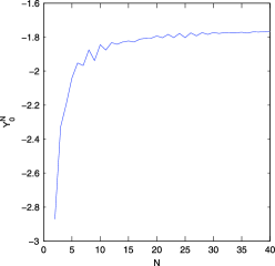
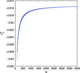
(a)	(b)

Figure 1: (a) $Y^{N}_{0}$ corresponding to $K_{1}=1$ and $K_{2}=1$. (b) $Y^{N}_{0}$ corresponding to $K_{1}=1$ and $K_{2}=5$.

Figure 1(a) and (b) show the convergence of $Y^{N}_{0}$ for different values of $K_{1}$ and $K_{2}$. It can be seen that for $(K_{1},K_{2})=(1,1)$, $Y^{N}_{0}$ converges rather fast. Already for $N=20$, it is close to the limit value. On the other hand, for $(K_{1},K_{2})=(1,5)$, the convergence is much slower.

6 Convergence results for convex drivers

In this section, we consider BS$\Delta$Es with drivers that are convex in $z$ and use convex duality to derive stronger convergence results than in Section 5. For the case where $f$ does not depend on $y$ it has been shown in Barrieu and El Karoui [2], Delbaen et al. [14] and Delbaen et al. [13] that BSDEs with convex drivers admit a convex dual representation. Here, we establish convex dual representations for solutions of BS$\Delta$Es and use them to show convergence. We need the following stronger version of condition (W1) on the approximating processes $W^{N}$:

1. [(W2)]

2. ${\mathbb{E}}[\Delta W^{N,k}_{t^{N}_{i}}\Delta W^{N,l}_{t^{N}_{i}}]=0$ for all $N\in\mathbb{N}$, $i=1,\ldots,i_{N}$, $k\neq l$ and

   $$\sup_{N,i,k}\frac{\|\Delta W^{N,k}_{t^{N}_{i}}\|_{\infty}}{\sqrt{\Delta\langle W^{N}\rangle_{t^{N}_{i}}}}<\infty.$$

Note that this implies (W1) for all $q\in[1,2)$. In the following, we assume that the drivers $f^{N}$ are convex in $z$ and define

$$g^{N}(t,y,\mu):=\mathop{\operatorname{ess}\sup}_{z}\bigl{\{}\mu z-f^{N}(t,y,z)\bigr{\}},\qquad\mu\in\mathbb{R}^{d}.$$

Let $\mu^{N}$ be an $\mathbb{R}^{d}$-valued $(\mathcal{F}^{N}_{t})$-adapted process that is constant on the intervals $(t^{N}_{i-1},t^{N}_{i}]$ and satisfies

$$\mu^{N}_{t^{N}_{i}}\Delta W^{N}_{t^{N}_{i}}>-1\qquad\mbox{for all }i.$$ (28)

Then

$$\frac{\mathrm{d}\mathbb{P}^{\mu^{N}}}{\mathrm{d}\mathbb{P}}=\prod_{i=1}^{i_{N}}\bigl{(}1+\mu^{N}_{t^{N}_{i}}\Delta W^{N}_{t^{N}_{i}}\bigr{)}$$ (29)

defines a probability measure $\mathbb{P}^{\mu^{N}}$ equivalent to $\mathbb{P}$ under which the processes

$$W^{N,\mu^{N},k}_{t^{N}_{i}}=W^{N,k}_{t^{N}_{i}}-\sum_{j=1}^{i}\mu^{k}_{t^{N}_{j}}\Delta\bigl{\langle}W^{N}\bigr{\rangle}_{t^{N}_{j}},\qquad k=1,\ldots,d,$$

are martingales. The following proposition gives an implicit dual representation of solutions of BS$\Delta$Es. Its proof can be found in the Appendix.

Proposition 6.1.

Assume (W2) and let $C,K,L\in\mathbb{R}_{+}$, $q\in[1,2)$ be constants such that all terminal conditions $\xi^{N}$ and drivers $f^{N}$ fulfill the following conditions:

1. [(iii)]

2. $\|\xi^{N}\|_{\infty}\leq C$;

3. $f^{N}$ is convex in $z$;

4. $|f^{N}(t,y,z)|\leq K(1+|y|+|z|^{q})$ for all $(t,y,z)\in[0,T]\times\mathbb{R}^{d+1}$;

5. $|f^{N}(t,y_{1},z)-f^{N}(t,y_{2},z)|\leq L|y_{1}-y_{2}|$ for all $(t,y,z)\in[0,T]\times\mathbb{R}^{d+1}$;

6. $|f^{N}(t,y,z_{1})-f^{N}(t,y,z_{2})|\leq L(1+(|z_{1}|\vee|z_{2}|)^{q/2})|z_{1}-z_{2}|$ for all $(t,y,z_{1},z_{2})\in[0,T]\times\mathbb{R}^{2d+1}$ such that $|y|\leq(C+1)\exp(KT)$.

Then there exists $N_{0}\in\mathbb{N}$ such that for every $N\geq N_{0}$, the $N$th BS$\Delta$E has a unique solution $(Y^{N},Z^{N},M^{N})$ and $Y^{N}$ can be represented as

$$Y^{N}_{t^{N}_{i}}=\mathop{\operatorname{ess}\sup}_{\mu^{N}}\mathbb{E}^{\mu^{N}}\Biggl{[}\xi^{N}-\sum_{j=i+1}^{i_{N}}g^{N}\bigl{(}t^{N}_{j},Y^{N}_{t^{N}_{j-1}},\mu^{N}_{t^{N}_{j}}\bigr{)}\Delta\bigl{\langle}W^{N}\bigr{\rangle}_{t^{N}_{j}}\Big{|}\mathcal{F}^{N}_{t^{N}_{i}}\Biggr{]},$$ (30)

where the essential supremum is taken over all $\mathbb{R}^{d}$-valued $(\mathcal{F}^{N}_{t})$-adapted processes $\mu^{N}$ that are constant on the intervals $(t^{N}_{i-1},t^{N}_{i}]$ and satisfy (28). Moreover, there exists a constant $R\in\mathbb{R}_{+}$ such that for each $N\geq N_{0}$, (30) admits a maximizer $\hat{\mu}^{N}$ satisfying

$$\mathbb{E}^{\hat{\mu}^{N}}\Biggl{[}\sum_{j=i+1}^{i_{N}}|\hat{\mu}_{t^{N}_{j}}|^{2}\Delta\bigl{\langle}W^{N}\bigr{\rangle}_{t^{N}_{j}}\Big{|}\mathcal{F}^{N}_{t^{N}_{i}}\Biggr{]}\leq R\qquad\mbox{for all }i\leq i_{N}-1.$$ (31)

We are now ready to prove our convergence result for convex drivers. It states that for any sequence of bounded discrete-time terminal conditions converging to $\xi$ and every sequence of discrete-time drivers converging to $f$ the discrete-time solutions $Y^{N}$ converge to the continuous-time solution $Y$.

Theorem 6.2

Assume (W2), the $f^{N}(t,y,z)$ are convex in $z$ and one has $\sup_{N}\|\xi^{N}\|_{\infty}<\infty$ as well as $\xi^{N}\to\xi$ in $L^{2}$. Moreover, suppose the $f^{N}$ satisfy (f1)–(f5). Then for $N$ large enough, the $N$th BS$\Delta$E has a unique solution $(Y^{N},Z^{N},M^{N})$ and

$$\sup_{t}\bigl{|}Y^{N}_{t}-Y_{t}\bigr{|}\rightarrow 0\qquad\mbox{in $L^{2}$ for }N\to\infty,$$

where $(Y,Z)$ is the unique solution of the BSDE (4) with bounded $Y$.

Proof.

By Theorem 5.9, there exist $\mathcal{F}^{N}_{T}$-measurable terminal conditions $\tilde{\xi}^{N}$ bounded by $C:=\sup_{N}\|\xi^{N}\|_{\infty}$ such that the corresponding solutions satisfy

$$\sup_{t}\bigl{|}\tilde{Y}^{N}_{t}-Y_{t}\bigr{|}\to 0\qquad\mbox{in }L^{2}.$$

Choose $b\in\mathbb{R}_{+}$ such that condition (f3) holds for $a=(C+1)\exp(KT)$. Then the conditions of Theorem 4.2 and Proposition 6.1 are satisfied with $L=K\vee b$. Hence, there exists $N_{0}\in\mathbb{N}$ such that for all $N\geq N_{0}$, $\sup_{t}|Y^{N}_{t}|$ and $\sup_{t}|\tilde{Y}^{N}_{t}|$ are bounded by $(C+1)\exp(KT)$ and

$$Y^{N}_{t^{N}_{i}} = \mathop{\operatorname{ess}\sup}_{\mu}{\mathbb{E}}^{\mu}\Biggl{[}\xi^{N}-\sum_{j=i+1}^{i_{N}}g^{N}\bigl{(}t^{N}_{j},Y^{N}_{t^{N}_{j-1}},\mu_{t^{N}_{j}}\bigr{)}\Delta\bigl{\langle}W^{N}\bigr{\rangle}_{t^{N}_{j}}\Big{|}\mathcal{F}^{N}_{t^{N}_{i}}\Biggr{]}$$

$$= \mathbb{E}^{\hat{\mu}^{N}}\Biggl{[}\xi^{N}-\sum_{j=i+1}^{i_{N}}g^{N}\bigl{(}t^{N}_{j},Y^{N}_{t^{N}_{j-1}},\hat{\mu}^{N}_{t^{N}_{j}}\bigr{)}\Delta\bigl{\langle}W^{N}\bigr{\rangle}_{t^{N}_{j}}\Big{|}\mathcal{F}^{N}_{t^{N}_{i}}\Biggr{]}$$

as well as

$$\tilde{Y}^{N}_{t^{N}_{i}} = \mathop{\operatorname{ess}\sup}_{\mu}{\mathbb{E}}^{\mu}\Biggl{[}\tilde{\xi}^{N}-\sum_{j=i+1}^{i_{N}}g^{N}\bigl{(}t^{N}_{j},\tilde{Y}^{N}_{t^{N}_{j-1}},\mu_{t^{N}_{j}}\bigr{)}\Delta\bigl{\langle}W^{N}\bigr{\rangle}_{t^{N}_{j}}\Big{|}\mathcal{F}^{N}_{t^{N}_{i}}\Biggr{]}$$

$$= \mathbb{E}^{\tilde{\mu}^{N}}\Biggl{[}\tilde{\xi}^{N}-\sum_{j=i+1}^{i_{N}}g^{N}\bigl{(}t^{N}_{j},\tilde{Y}^{N}_{t^{N}_{j-1}},\tilde{\mu}^{N}_{t^{N}_{j}}\bigr{)}\Delta\bigl{\langle}W^{N}\bigr{\rangle}_{t^{N}_{j}}\Big{|}\mathcal{F}^{N}_{t^{N}_{i}}\Biggr{]}.$$

If we can show

$$\sup_{t}\bigl{|}\tilde{Y}^{N}_{t}-Y^{N}_{t}\bigr{|}\to 0\qquad\mbox{in }L^{2},$$

we get

$$\sup_{t}\bigl{|}Y^{N}_{t}-Y_{t}\bigr{|}\to 0\qquad\mbox{in }L^{2},$$

and the theorem is proved. As the supremum of $K$-Lipschitz functions, $g^{N}$ is again $K$-Lipschitz in $y$. Hence, since $|\max\{a_{1},a_{2}\}-\max\{b_{1},b_{2}\}|\leq\max\{|a_{1}-b_{1}|,|a_{2}-b_{2}|\}$ for $a_{1},a_{2},b_{1},b_{2}\in\mathbb{R}$, and

$$Y^{N}_{t^{N}_{i}} = \max_{\mu\in\{\hat{\mu}^{N},\tilde{\mu}^{N}\}}{\mathbb{E}}^{\mu}\Biggl{[}\xi^{N}-\sum_{j=i+1}^{i_{N}}g^{N}\bigl{(}t^{N}_{j},Y^{N}_{t^{N}_{j-1}},\mu_{t^{N}_{j}}\bigr{)}\Delta\bigl{\langle}W^{N}\bigr{\rangle}_{t^{N}_{j}}\Big{|}\mathcal{F}^{N}_{t^{N}_{i}}\Biggr{]},$$

$$\tilde{Y}^{N}_{t^{N}_{i}} = \max_{\mu\in\{\hat{\mu}^{N},\tilde{\mu}^{N}\}}{\mathbb{E}}^{\mu}\Biggl{[}\tilde{\xi}^{N}-\sum_{j=i+1}^{i_{N}}g^{N}\bigl{(}t^{N}_{j},\tilde{Y}^{N}_{t^{N}_{j-1}},\mu_{t^{N}_{j}}\bigr{)}\Delta\bigl{\langle}W^{N}\bigr{\rangle}_{t^{N}_{j}}\Big{|}\mathcal{F}^{N}_{t^{N}_{i}}\Biggr{]},$$

one obtains

$$\bigl{|}\tilde{Y}^{N}_{t^{N}_{i}}-Y^{N}_{t^{N}_{i}}\bigr{|} \leq \max_{\mu\in\{\hat{\mu}^{N},\tilde{\mu}^{N}\}}{\mathbb{E}}^{\mu}\Biggl{[}\bigl{|}\tilde{\xi}^{N}-\xi^{N}\bigr{|}+K\sum_{j=i+1}^{i_{N}}\bigl{|}\tilde{Y}_{t^{N}_{j-1}}^{N}-Y^{N}_{t^{N}_{j-1}}\bigr{|}\Delta\bigl{\langle}W^{N}\bigr{\rangle}_{t^{N}_{j}}\Big{|}\mathcal{F}^{N}_{t^{N}_{i}}\Biggr{]}$$

$$\leq \mathbb{E}^{\hat{\mu}^{N}}\Biggl{[}\bigl{|}\tilde{\xi}^{N}-\xi^{N}\bigr{|}+K\sum_{j=i+1}^{i_{N}}\bigl{|}\tilde{Y}_{t^{N}_{j-1}}^{N}-Y^{N}_{t^{N}_{j-1}}\bigr{|}\Delta\bigl{\langle}W^{N}\bigr{\rangle}_{t^{N}_{j}}\Big{|}\mathcal{F}^{N}_{t^{N}_{i}}\Biggr{]}$$

$${}+\mathbb{E}^{\tilde{\mu}^{N}}\Biggl{[}\bigl{|}\tilde{\xi}^{N}-\xi^{N}\bigr{|}+K\sum_{j=i+1}^{i_{N}}\bigl{|}\tilde{Y}_{t^{N}_{j-1}}^{N}-Y^{N}_{t^{N}_{j-1}}\bigr{|}\Delta\bigl{\langle}W^{N}\bigr{\rangle}_{t^{N}_{j}}\Big{|}\mathcal{F}^{N}_{t^{N}_{i}}\Biggr{]}.$$

From Proposition 6.1, we know that there exists a constant $R\in\mathbb{R}_{+}$ such that

$$\mathbb{E}^{\hat{\mu}^{N}}\Biggl{[}\sum_{j=i+1}^{i_{N}}\bigl{|}\hat{\mu}^{N}_{t^{N}_{j}}\bigr{|}^{2}\Delta\bigl{\langle}W^{N}\bigr{\rangle}_{t^{N}_{j}}\Big{|}\mathcal{F}^{N}_{t^{N}_{i}}\Biggr{]}\leq R\qquad\mbox{for all }N\geq N_{0}\mbox{ and }i=0,\ldots,i_{N}-1.$$

Consequently, we obtain from Lemma .3 in the Appendix that there exists a constant $\tilde{R}$ such that

$${\mathbb{E}}\Biggl{[}\varphi\Biggl{(}\prod_{j=i+1}^{i_{N}}\bigl{(}1+\hat{\mu}^{N}_{t^{N}_{j}}\Delta W^{N}_{t^{N}_{j}}\bigr{)}\Biggr{)}\Big{|}\mathcal{F}^{N}_{t^{N}_{i}}\Biggr{]}\leq\tilde{R}\qquad\mbox{for all }N\geq N_{0}\mbox{ and }i=0,\ldots,i_{N}-1,$$

where $\varphi(x)=x\log(x)\vee 1$. Fix $\varepsilon>0$ and set $D=2[C+(C+1)\exp(KT)K\sup_{N\geq N_{0}}\langle W^{N}\rangle_{T}]$. Since $\varphi(x)/x\uparrow\infty$, there exists $B\in\mathbb{R}_{+}$ such that for all $x>B$,

$$\frac{x}{\varphi(x)}\leq\frac{\varepsilon}{\tilde{R}D}.$$

Introduce the sets $E^{N}_{i+1}=\{\prod_{j=i+1}^{i_{N}}(1+\hat{\mu}^{N}_{t^{N}_{j}}\Delta W^{N}_{t^{N}_{j}})>B\}$. Then

$$\sup_{N\geq N_{0},0\leq i\leq i_{N}-1}\mathbb{E}\Biggl{[}1_{E^{N}_{i+1}}\prod_{j=i+1}^{i_{N}}\bigl{(}1+\hat{\mu}^{N}_{t^{N}_{j}}\Delta W^{N}_{t^{N}_{j}}\bigr{)}\Big{|}\mathcal{F}^{N}_{t^{N}_{i}}\Biggr{]}$$

$$\quad=\sup_{N\geq N_{0},0\leq i\leq i_{N}-1}{\mathbb{E}}\Biggl{[}1_{E^{N}_{i+1}}\frac{\prod_{j=i+1}^{i_{N}}(1+\hat{\mu}^{N}_{t^{N}_{j}}\Delta W^{N}_{t^{N}_{j}})}{\varphi(\prod_{j=i+1}^{i_{N}}(1+\hat{\mu}^{N}_{t^{N}_{j}}\Delta W^{N}_{t^{N}_{j}}))}$$ (32)

$$\hskip 92.0pt{}\times\varphi\Biggl{(}\prod_{j=i+1}^{i_{N}}\bigl{(}1+\hat{\mu}^{N}_{t^{N}_{j}}\Delta W^{N}_{t^{N}_{j}}\bigr{)}\Biggr{)}\Big{|}\mathcal{F}^{N}_{t^{N}_{i}}\Biggr{]}$$

$$\quad\leq\frac{\varepsilon}{\tilde{R}D}\sup_{N\geq N_{0},0\leq i\leq i_{N}-1}{\mathbb{E}}\Biggl{[}\varphi\Biggl{(}\prod_{j=i+1}^{i_{N}}\bigl{(}1+\hat{\mu}^{N}_{t^{N}_{j}}\Delta W^{N}_{t^{N}_{j}}\bigr{)}\Biggr{)}\Big{|}\mathcal{F}^{N}_{t^{N}_{i}}\Biggr{]}\leq\frac{\varepsilon}{D}.$$

This yields for all $N\geq N_{0}$,

$$\mathbb{E}^{\hat{\mu}^{N}}\Biggl{[}\bigl{|}\tilde{\xi}^{N}-\xi^{N}\bigr{|}+K\sum_{j=i+1}^{i_{N}}\bigl{|}\tilde{Y}_{t^{N}_{j-1}}^{N}-Y^{N}_{t^{N}_{j-1}}\bigr{|}\Delta\bigl{\langle}W^{N}\bigr{\rangle}_{t^{N}_{j}}|\mathcal{F}^{N}_{t^{N}_{i}}\Biggr{]}$$

$$\quad=\mathbb{E}\Biggl{[}\prod_{j=i+1}^{i_{N}}\bigl{(}1+\hat{\mu}^{N}_{t^{N}_{j}}\Delta W^{N}_{t^{N}_{j}}\bigr{)}\Biggl{(}\bigl{|}\tilde{\xi}^{N}-\xi^{N}\bigr{|}+K\sum_{j=i+1}^{i_{N}}\bigl{|}\tilde{Y}_{t^{N}_{j-1}}^{N}-Y^{N}_{t^{N}_{j-1}}\bigr{|}\Delta\bigl{\langle}W^{N}\bigr{\rangle}_{t^{N}_{j}}\Biggr{)}\Big{|}\mathcal{F}^{N}_{t^{N}_{i}}\Biggr{]}$$

$$\quad=\mathbb{E}\Biggl{[}1_{E^{N}_{i+1}}\prod_{j=i+1}^{i_{N}}\bigl{(}1+\hat{\mu}^{N}_{t^{N}_{j}}\Delta W^{N}_{t^{N}_{j}}\bigr{)}\Biggl{(}\bigl{|}\tilde{\xi}^{N}-\xi^{N}\bigr{|}+K\sum_{j=i+1}^{i_{N}}\bigl{|}\tilde{Y}_{t^{N}_{j-1}}^{N}-Y^{N}_{t^{N}_{j-1}}\bigr{|}\Delta\bigl{\langle}W^{N}\bigr{\rangle}_{t^{N}_{j}}\Biggr{)}\Big{|}\mathcal{F}^{N}_{t^{N}_{i}}\Biggr{]}$$

$$\qquad{}+\mathbb{E}\Biggl{[}1_{E^{N,c}_{i+1}}\prod_{j=i+1}^{i_{N}}\bigl{(}1+\hat{\mu}^{N}_{t^{N}_{j}}\Delta W^{N}_{t^{N}_{j}}\bigr{)}\Biggl{(}\bigl{|}\tilde{\xi}^{N}-\xi^{N}\bigr{|}+K\sum_{j=i+1}^{i_{N}}\bigl{|}\tilde{Y}_{t^{N}_{j-1}}^{N}-Y^{N}_{t^{N}_{j-1}}\bigr{|}\Delta\bigl{\langle}W^{N}\bigr{\rangle}_{t^{N}_{j}}\Biggr{)}\Big{|}\mathcal{F}^{N}_{t^{N}_{i}}\Biggr{]}$$

$$\quad\leq D{\mathbb{E}}\Biggl{[}1_{E^{N}_{i+1}}\prod_{j=i+1}^{i_{N}}\bigl{(}1+\hat{\mu}^{N}_{t^{N}_{j}}\Delta W^{N}_{t^{N}_{j}}\bigr{)}|\mathcal{F}^{N}_{t^{N}_{i}}\Biggr{]}$$

$$\qquad{}+\mathbb{E}\Biggl{[}1_{E^{N,c}_{t^{N}_{i+1}}}\prod_{j=i+1}^{i_{N}}\bigl{(}1+\hat{\mu}^{N}_{t^{N}_{j}}\Delta W^{N}_{t^{N}_{j}}\bigr{)}$$

$$\hskip 92.0pt{}\times\Biggl{(}\bigl{|}\tilde{\xi}^{N}-\xi^{N}\bigr{|}+K\sum_{j=i+1}^{i_{N}}\bigl{|}\tilde{Y}_{t^{N}_{j-1}}^{N}-Y^{N}_{t^{N}_{j-1}}\bigr{|}\Delta\bigl{\langle}W^{N}\bigr{\rangle}_{t^{N}_{j}}\Biggr{)}\Big{|}\mathcal{F}^{N}_{t^{N}_{i}}\Biggr{]}$$

$$\quad\leq\varepsilon+B{\mathbb{E}}\Biggl{[}\bigl{|}\tilde{\xi}^{N}-\xi^{N}\bigr{|}+K\sum_{j=i+1}^{i_{N}}\bigl{|}\tilde{Y}_{t^{N}_{j-1}}^{N}-Y^{N}_{t^{N}_{j-1}}\big{|}\Delta\bigl{\langle}W^{N}\bigr{\rangle}_{t^{N}_{j}}\Big{|}\mathcal{F}^{N}_{t^{N}_{i}}\Biggr{]}.$$

In the first inequality, we used that the random variables $|\tilde{\xi}^{N}-\xi^{N}|+K\sum_{j=i+1}^{i_{N}}|\tilde{Y}_{t^{N}_{j-1}}^{N}-Y^{N}_{t^{N}_{j-1}}|\Delta\langle W^{N}\rangle_{t^{N}_{j}}$ are uniformly bounded by $D$. In the second inequality, we used (6) and the definition of the sets $E^{N}_{i+1}$. Using the same estimate for $\tilde{\mu}^{N}$ instead of $\hat{\mu}^{N}$ gives

$$\bigl{|}\tilde{Y}^{N}_{t^{N}_{i}}-Y^{N}_{t^{N}_{i}}\bigr{|}\leq 2\varepsilon+2B\mathbb{E}\Biggl{[}\bigl{|}\tilde{\xi}^{N}-\xi^{N}\bigr{|}+K\sum_{j=i+1}^{i_{N}}\bigl{|}\tilde{Y}_{t^{N}_{j-1}}^{N}-Y^{N}_{t^{N}_{j-1}}\bigr{|}\Delta\bigl{\langle}W^{N}\bigr{\rangle}_{t^{N}_{j}}\Big{|}\mathcal{F}^{N}_{t^{N}_{i}}\Biggr{]}.$$ (33)

Taking expectations, one gets

$$\mathbb{E}\bigl{[}\bigl{|}\tilde{Y}^{N}_{t^{N}_{i}}-Y^{N}_{t^{N}_{i}}\bigr{|}\bigr{]}\leq 2\varepsilon+2B{\mathbb{E}}\bigl{[}\bigl{|}\tilde{\xi}^{N}-\xi^{N}\bigr{|}\bigr{]}+K\sum_{j=i+1}^{i_{N}}{\mathbb{E}}\bigl{[}\bigl{|}\tilde{Y}^{N}_{t^{N}_{j-1}}-Y^{N}_{t^{N}_{j-1}}\bigr{|}\bigr{]}\Delta\bigl{\langle}W^{N}\bigr{\rangle}_{t^{N}_{j}}.$$

Since $\varepsilon>0$ was arbitrary, one obtains from a discrete version of Gronwall’s lemma (see Lemma .4 in the Appendix) that

$$\sup_{t}{\mathbb{E}}\bigl{[}\bigl{|}\tilde{Y}^{N}_{t}-Y^{N}_{t}\bigr{|}\bigr{]}\to 0\qquad\mbox{as }N\to\infty,$$

and since $Y^{N}$ and $\tilde{Y}^{N}$ are both bounded by $(C+1)\exp(KT)$, also

$$\sup_{t}{\mathbb{E}}\bigl{[}\bigl{|}\tilde{Y}^{N}_{t}-Y^{N}_{t}\bigr{|}^{2}\bigr{]}\to 0\qquad\mbox{as }N\to\infty.$$ (34)

It remains to show that $\sup_{t}$ can be taken inside of the expectation in (34). To do this, note that (33) gives

$$\sup_{i}\bigl{|}\tilde{Y}_{t^{N}_{i}}^{N}-Y^{N}_{t^{N}_{i}}\bigr{|}\leq 2\varepsilon+2B\Bigl{(}\sup_{i}{\mathbb{E}}\bigl{[}\bigl{|}\tilde{\xi}^{N}-\xi^{N}\bigr{|}|\mathcal{F}^{N}_{t^{N}_{i}}\bigr{]}+K\sup_{i}A^{N}_{t^{N}_{i}}\Bigr{)}$$

for the nonnegative martingale

$$A^{N}_{t^{N}_{i}}={\mathbb{E}}\Biggl{[}\sum_{j=1}^{i_{N}}\bigl{|}\tilde{Y}_{t^{N}_{j-1}}^{N}-Y^{N}_{t^{N}_{j-1}}\bigr{|}\Delta\bigl{\langle}W^{N}\bigr{\rangle}_{t^{N}_{j}}\Big{|}\mathcal{F}^{N}_{t^{N}_{i}}\Biggr{]},\qquad i=0,\ldots,i_{N}.$$

Since $\varepsilon$ was arbitrary, and $\sup_{i}{\mathbb{E}}[|\tilde{\xi}^{N}-\xi^{N}||\mathcal{F}^{N}_{t^{N}_{i}}]\stackrel{{\scriptstyle(N\rightarrow\infty)}}{{\to}}0$ in $L^{2}$ by Doob’s maximal inequality, the only thing left to show is $\sup_{i}A^{N}_{t^{N}_{i}}\stackrel{{\scriptstyle(N\rightarrow\infty)}}{{\to}}0$ in $L^{2}.$ Applying Doob’s maximal inequality to $A^{N}$ yields

$${\mathbb{E}}\Bigl{[}\sup_{i}\bigl{|}A^{N}_{t^{N}_{i}}\bigr{|}^{2}\Bigr{]} \leq 2{\mathbb{E}}\Biggl{[}\Biggl{(}\sum_{j=1}^{i_{N}}\bigl{|}\tilde{Y}_{t^{N}_{j-1}}^{N}-Y^{N}_{t^{N}_{j-1}}\bigr{|}\Delta\bigl{\langle}W^{N}\bigr{\rangle}_{t^{N}_{j}}\Biggr{)}^{2}\Biggr{]}$$

$$\leq 2\bigl{\langle}W^{N}\bigr{\rangle}_{T}{\mathbb{E}}\Biggl{[}\sum_{j=1}^{i_{N}}\bigl{|}\tilde{Y}^{N}_{t^{N}_{j-1}}-Y^{N}_{t^{N}_{j-1}}\bigr{|}^{2}\Delta\bigl{\langle}W^{N}\bigr{\rangle}_{t^{N}_{j}}\Biggr{]}$$

$$\leq 2\bigl{(}\bigl{\langle}W^{N}\bigr{\rangle}_{T}\bigr{)}^{2}\sup_{t}{\mathbb{E}}\bigl{[}\bigl{|}\tilde{Y}^{N}_{t}-Y^{N}_{t}\bigr{|}^{2}\bigr{]}\rightarrow 0\qquad\mbox{as }N\rightarrow\infty,$$

where we used Jensen’s inequality for the second inequality and (34) for the convergence in the last line. This proves the theorem. ∎

If one has convergence of $(W^{N},\xi^{N})$ to $(W,\xi)$ in distribution instead of $L^{2}$ together with

$$\sup_{N}{\mathbb{E}}\Bigl{[}\sup_{t}\bigl{|}W^{N}_{t}\bigr{|}^{2+\varepsilon}\Bigr{]}<\infty\quad\mbox{and}\quad\sup_{N}\bigl{\|}\xi^{N}\bigr{\|}_{\infty}<\infty,$$

one can show as in Example 2.1 that there exists a probability space $(\tilde{\Omega},\tilde{\mathcal{F}},\tilde{\mathbb{P}})$ carrying $(\tilde{W}^{N},\tilde{\xi}^{N})$ distributed as $(W^{N},\xi^{N})$ and $(\tilde{W},\tilde{\xi})$ distributed as $(W,\xi)$ such that

$${\mathbb{E}}\Bigl{[}\sup_{t}\bigl{|}\tilde{W}^{N}_{t}-\tilde{W}_{t}\bigr{|}^{2}\Bigr{]}\to 0\quad\mbox{and}\quad{\mathbb{E}}\bigl{[}\bigl{|}\tilde{\xi}^{N}-\tilde{\xi}\bigr{|}^{2}\bigr{]}\to 0\qquad\mbox{for }N\to\infty.$$

In the case where the drivers $f$ and $f^{N}$ are given as in (22) and (27), the following holds.

Corollary 6.3.

Assume the $W^{N}$ fulfill (C1), (C2) and (W2), but instead of (C3), $(W^{N},\xi^{N})$ converges in distribution to $(W,\xi)$ and one has $\sup_{N}{\mathbb{E}}[\sup_{t}|W^{N}_{t}|^{2+\varepsilon}]<\infty$ for some $\varepsilon>0$ and $\sup_{N}\|\xi^{N}\|_{\infty}<\infty$. Furthermore, suppose $f$ and $f^{N}$ are of the form (22) and (27), respectively. Then for $N$ large enough, the $N$th BS$\Delta$E has a unique solution $(Y^{N},Z^{N},M^{N})$ and

$$\sup_{t}\bigl{|}Y^{N}_{t}-Y_{t}\bigr{|}\to 0\qquad\mbox{in distribution for }N\to\infty,$$

where $(Y,Z)$ is the unique solution of the BSDE (4) with bounded $Y$.

Appendix

.1 Proofs of Section 3

Proof of Lemma 3.1 If $(Y^{N},Z^{N},M^{N})$ is a solution of the $N$th BS$\Delta$E, then

$$Y^{N}_{t^{N}_{i}}-f^{N}\bigl{(}t^{N}_{i+1},Y^{N}_{t^{N}_{i}},Z^{N}_{t^{N}_{i+1}}\bigr{)}\Delta\bigl{\langle}W^{N}\bigr{\rangle}_{t^{N}_{i+1}}+Z^{N}_{t^{N}_{i+1}}\Delta W^{N}_{t^{N}_{i+1}}+\Delta M^{N}_{t^{N}_{i+1}}=Y^{N}_{t^{N}_{i+1}}.$$ (1)

Taking conditional expectations on both sides with respect to $\mathcal{F}^{N}_{t^{N}_{i}}$ gives (8). Multiplying both sides of (1) with $\Delta W^{N,k}_{t^{N}_{i+1}}$ and taking conditional expectations with respect to $\mathcal{F}^{N}_{t^{N}_{i}}$ yields (9). Finally, (10) is a consequence of (8) and (1).

Proof of Proposition 3.2 We prove the proposition by backwards induction. Set $Y^{N}_{T}=\xi^{N}$, which by assumption (C4) is bounded. Now assume that there exist $i$ and $(Y^{N}_{t},Z^{N}_{t},M^{N}_{t})$ solving the BS$\Delta$E (5) for $t\in[t^{N}_{i+1},T]$ such that $(Y^{N}_{t})$ and $(Z^{N}_{t})$ are bounded. By Lemma 3.1, $Z^{N,k}_{t^{N}_{i+1}}$ must be of the form

$$Z^{N,k}_{t^{N}_{i+1}}=\frac{{\mathbb{E}}[Y^{N}_{t^{N}_{i+1}}\Delta W^{N,k}_{t^{N}_{i+1}}|\mathcal{F}^{N}_{t^{N}_{i}}]}{\Delta\langle W^{N}\rangle_{t^{N}_{i+1}}}.$$

Since by induction hypothesis, $Y^{N}_{t^{N}_{i+1}}$ is bounded, $Z^{N,k}_{t^{N}_{i+1}}$ is well-defined and bounded. Next, we try to find $Y^{N}_{t^{N}_{i}}\in L^{\infty}(\mathcal{F}^{N}_{t^{N}_{i}})$ such that

$$Y^{N}_{t^{N}_{i}}-f^{N}\bigl{(}t^{N}_{i+1},Y^{N}_{t^{N}_{i}},Z^{N}_{t^{N}_{i+1}}\bigr{)}\Delta\bigl{\langle}W^{N}\bigr{\rangle}_{t^{N}_{i+1}}={\mathbb{E}}\bigl{[}Y^{N}_{t^{N}_{i+1}}|\mathcal{F}^{N}_{t^{N}_{i}}\bigr{]}.$$ (2)

To do that, we introduce the mapping $A(\omega,y):=y-f(t^{N}_{i+1},y,Z^{N}_{t^{N}_{i+1}})\Delta\langle W^{N}\rangle_{t^{N}_{i+1}}$. It is $\mathcal{F}^{N}_{t^{N}_{i}}$-measurable in $\omega$ and continuous in $y$. Moreover, it satisfies

$$y-\kappa\bigl{(}1+|y|+g\bigl{(}Z^{N}_{t^{N}_{i+1}}\bigr{)}\bigr{)}\leq A(\omega,y)\leq y+\kappa\bigl{(}1+|y|+g\bigl{(}Z^{N}_{t^{N}_{i+1}}\bigr{)}\bigr{)}$$ (3)

for $\kappa=K\max_{i}\Delta\langle W^{N}\rangle_{t^{N}_{i}}<1$. So it follows from Lemma .1 below that there exists an $\mathcal{F}^{N}_{t^{N}_{i}}\otimes\mathcal{B}(\mathbb{R})$-measurable function $B\mathchoice{\nobreak\,\colon}{\nobreak\,\colon}{\nobreak\,\colon\;}{\nobreak\,\colon\;}\Omega\times\mathbb{R}\rightarrow\mathbb{R}$ such that $A(\omega,B(\omega,y))=y$ for all $(\omega,y)\in\Omega\times\mathbb{R}$. Thus,

$$Y^{N}_{t^{N}_{i}}=B\bigl{(}\omega,{\mathbb{E}}\bigl{[}Y^{N}_{t^{N}_{i+1}}|\mathcal{F}^{N}_{t^{N}_{i}}\bigr{]}\bigr{)}\in L^{0}\bigl{(}\mathcal{F}^{N}_{t^{N}_{i}}\bigr{)}$$

solves (2), and since $Y^{N}_{t^{N}_{i+1}}$ and $Z^{N}_{t^{N}_{i+1}}$ are bounded, it follows from the estimate (3) that the same is true for $Y^{N}_{t^{N}_{i}}$. Finally, $M^{N}_{0}=0$ and

$$\Delta M^{N}_{t^{N}_{i+1}} = \Delta Y^{N}_{t^{N}_{i+1}}+f^{N}\bigl{(}t^{N}_{i+1},Y^{N}_{t^{N}_{i}},Z^{N}_{t^{N}_{i+1}}\bigr{)}\Delta\bigl{\langle}W^{N}\bigr{\rangle}_{t^{N}_{i+1}}-Z^{N}_{t^{N}_{i+1}}\Delta W^{N}_{t^{N}_{i+1}}$$

$$= Y^{N}_{t^{N}_{i+1}}-{\mathbb{E}}\bigl{[}Y^{N}_{t^{N}_{i+1}}|\mathcal{F}^{N}_{t^{N}_{i}}\bigr{]}-Z^{N}_{t^{N}_{i+1}}\Delta W^{N}_{t^{N}_{i+1}}$$

defines a square-integrable martingale $M^{N}$ orthogonal to $W^{N}$ which is bounded if $W^{N}$ is so. This completes the proof.

Lemma .1.

Let $\mathcal{G}$ be a sub-$\sigma$-algebra of $\mathcal{F}$ and $A\mathchoice{\nobreak\,\colon}{\nobreak\,\colon}{\nobreak\,\colon\;}{\nobreak\,\colon\;}\Omega\times\mathbb{R}\to\mathbb{R}$ a function that is $\mathcal{G}$-measurable in $\omega\in\Omega$ and continuous in $y\in\mathbb{R}$. Assume that for every $\omega\in\Omega$, the set $\{y\in\mathbb{R}\colon\ A(\omega,y)\in C\}$ is nonempty and bounded for each nonempty bounded subset $C$ of $\mathbb{R}$. Then there exists a $\mathcal{G}\otimes\mathcal{B}(\mathbb{R})$-measurable function $B\mathchoice{\nobreak\,\colon}{\nobreak\,\colon}{\nobreak\,\colon\;}{\nobreak\,\colon\;}\Omega\times\mathbb{R}\to\mathbb{R}$ such that $A(\omega,B(\omega,x))=x$ for all $x\in\mathbb{R}$.

Proof.

For all $k,l\in\mathbb{N}$,

$$b_{kl}(\omega)=\inf\bigl{\{}y\in\mathbb{R}\colon\ A(\omega,y)\in\bigl{(}(k-1)2^{-l},k2^{-l}\bigr{]}\bigr{\}}$$

is a $\mathcal{G}$-measurable mapping from $\Omega$ to $\mathbb{R}$ and

$$B_{l}(\omega,x)=\sum_{k\in\mathbb{Z}}b_{kl}(\omega)1_{\{(k-1)2^{-l}<x\leq k2^{-l}\}}$$

a $\mathcal{G}\otimes\mathcal{B}(\mathbb{R})$-measurable map from $\Omega\times\mathbb{R}$ to $\mathbb{R}$ such that

$$B_{l}(\omega,x)\to B(\omega,x)\qquad\mbox{as }l\to\infty$$

for a $\mathcal{G}\otimes\mathcal{B}(\mathbb{R})$-measurable function $B:\Omega\times\mathbb{R}\to\mathbb{R}$. Since $y\mapsto A(\omega,y)$ is continuous for all $\omega\in\Omega$, one obtains

$$A\bigl{(}\omega,B(\omega,x)\bigr{)}=A\Bigl{(}\omega,\lim_{l\to\infty}B_{l}(\omega,x)\Bigr{)}=\lim_{l\to\infty}A\bigl{(}\omega,B_{l}(\omega,x)\bigr{)}=x$$

for all $x\in\mathbb{R}$. ∎

.2 Proofs of Lemmas 4.3 and 4.4

To prove Lemmas 4.3 and 4.4, we need the following lemma.

Lemma .2.

Assume the $N$th driver and terminal condition are of the special form

$$f^{N}(t,y,z)=K\bigl{(}1+|y|+g(z)\bigr{)}\quad\mbox{and}\quad\xi^{N}=C$$

for constants $C,K\in\mathbb{R}_{+}$ and a measurable function $g\mathchoice{\nobreak\,\colon}{\nobreak\,\colon}{\nobreak\,\colon\;}{\nobreak\,\colon\;}\mathbb{R}^{d}\to\mathbb{R}$ with $g(0)=0$. Then for all $N\in\mathbb{N}$ such that $\max_{i}\Delta\langle W^{N}\rangle_{t^{N}_{i}}<1/K$, the $N$th BS$\Delta$E has a unique solution $(Y^{N},Z^{N},M^{N})$ given by

$$Y^{N}_{T}=C,\qquad Y^{N}_{t^{N}_{i}}=\frac{Y^{N}_{t^{N}_{i+1}}+K\Delta\langle W^{N}\rangle_{t^{N}_{i+1}}}{1-K\Delta\langle W^{N}\rangle_{t^{N}_{i+1}}},\qquad Z^{N}_{t^{N}_{i}}=0,\qquad M^{N}_{t^{N}_{i}}=0.$$ (4)

In particular, $Y^{N}$ is deterministic and for $N\to\infty$, converges uniformly to the function

$$(C+1)\exp\bigl{(}K(T-t)\bigr{)}-1.$$

Proof.

Since the terminal condition and the increments $\Delta\langle W^{N}\rangle_{t^{N}_{i}}$ are deterministic, $Z^{N}$ and $M^{N}$ are both zero and $Y^{N}$ solves

$$Y^{N}_{t^{N}_{i}}=Y^{N}_{t^{N}_{i+1}}+K\bigl{(}1+\bigl{|}Y^{N}_{t^{N}_{i}}\bigr{|}\bigr{)}\Delta\bigl{\langle}W^{N}\bigr{\rangle}_{t^{N}_{i+1}},\qquad Y^{N}_{T}=C.$$ (5)

This shows (4). Moreover, since (5) are deterministic difference equations with Lipschitz coefficients, one obtains from Theorem 2.2 that their solutions converge uniformly to the solution of the ordinary differential equation

$$y^{\prime}(t)=-K\bigl{(}1+\bigl{|}y(t)\bigr{|}\bigr{)},\qquad y(T)=C,$$

given by

$$y(t)=(C+1)\exp\bigl{(}K(T-t)\bigr{)}-1.$$

$$\eqntext{\qed}$$ (6)

∎

Proof of Lemma 4.3 Since $\max_{i}\Delta\langle W^{N}\rangle_{t^{N}_{i}}<1/K$ for $N$ large enough, it follows from Lemma .2 that there exists an $N_{1}\geq 1$ such that for all $N\geq N_{1}$, the BS$\Delta$E with driver $\hat{f}^{N}(t,y,z)=K(1+|y|+|z|^{q})$ and terminal condition $\hat{\xi}^{N}=C$ has a deterministic solution $\hat{Y}^{N}$ that is bounded by $(C+1)\exp(K(T-t))$. Set $D=2(C+1)\exp(KT)$. Since $q<2$, one obtains from condition (C5) that there exists $N_{0}\geq N_{1}$ such that

$$\sup_{N\geq N_{0}}\max_{i}K\bigl{(}1+d^{q/2}D^{q}\bigl{[}\Delta\bigl{\langle}W^{N}\bigr{\rangle}_{t^{N}_{i}}\bigr{]}^{-q/2}\bigr{)}\Delta\bigl{\langle}W^{N}\bigr{\rangle}_{t^{N}_{i}}<1$$ (7)

and

$$\sup_{N\geq N_{0}}\max_{i,k}dqK\bigl{(}1+d^{q/4}D^{q/2}\bigl{[}\Delta\bigl{\langle}W^{N}\bigr{\rangle}_{t^{N}_{i}}\bigr{]}^{-q/4}\bigr{)}\bigl{\|}\Delta W^{N,k}_{t^{N}_{i}}\bigr{\|}_{\infty}\leq 1.$$ (8)

Fix $N\geq N_{0}$ and let $f^{N}_{1}\geq f^{N}_{2}$ be drivers and $\xi^{N}_{1}\geq\xi^{N}_{2}$ terminal conditions satisfying assumptions (i)–(iv) of Lemma 4.3. By Proposition 3.2, both BS$\Delta$Es have a solution $(Y^{N}_{m},Z^{N}_{m},M^{N}_{m})$, $m=1,2$, and (13) clearly holds at the final time $T$. We now go backwards in time and assume (13) is true on $[t_{i+1},T]$. Then

$$(C+1)\exp\bigl{(}K\bigl{(}T-{t^{N}_{i+1}}\bigr{)}\bigr{)}\geq Y^{N}_{1,t^{N}_{i+1}}\geq Y^{N}_{2,t^{N}_{i+1}}\geq-(C+1)\exp\bigl{(}K\bigl{(}T-{t^{N}_{i+1}}\bigr{)}\bigr{)}.$$ (9)

By Lemma 3.1, one has

$$Z^{N,k}_{m,t^{N}_{i+1}}=\frac{{\mathbb{E}}[Y^{N}_{m,t^{N}_{i+1}}\Delta W^{N,k}_{t^{N}_{i+1}}|\mathcal{F}^{N}_{t^{N}_{i}}]}{\Delta\langle W^{N}\rangle_{t^{N}_{i+1}}},$$ (10)

and

$$Y^{N}_{m,t^{N}_{i}}={\mathbb{E}}\bigl{[}Y^{N}_{m,t^{N}_{i+1}}|\mathcal{F}^{N}_{t^{N}_{i}}\bigr{]}+f^{N}_{m}\bigl{(}t^{N}_{i+1},Y^{N}_{m,t^{N}_{i}},Z^{N}_{m,t^{N}_{i+1}}\bigr{)}\Delta\bigl{\langle}W^{N}\bigr{\rangle}_{t^{N}_{i+1}}.$$

Set

$$Y^{N}_{t}:=Y^{N}_{1,t}-Y^{N}_{2,t},\qquad Z^{N}_{t}:=Z^{N}_{1,t}-Z^{N}_{2,t}.$$

By (9), $Y^{N}_{1,t^{N}_{i+1}}$, $Y^{N}_{2,t^{N}_{i+1}}$ and $Y^{N}_{t^{N}_{i+1}}$ are bounded by $D$ and

$$Y^{N}_{t^{N}_{i}}={\mathbb{E}}\bigl{[}Y^{N}_{t^{N}_{i+1}}|\mathcal{F}^{N}_{t^{N}_{i+1}}\bigr{]}+\bigl{(}\alpha+Y^{N}_{t^{N}_{i}}\beta+Z^{N}_{t^{N}_{i+1}}\gamma\bigr{)}\Delta\bigl{\langle}W^{N}\bigr{\rangle}_{t^{N}_{i+1}}$$

for

$$\alpha = f^{N}_{1}\bigl{(}t^{N}_{i+1},Y^{N}_{2,t^{N}_{i}},Z^{N}_{2,t^{N}_{i+1}}\bigr{)}-f^{N}_{2}\bigl{(}t^{N}_{i+1},Y^{N}_{2,t^{N}_{i}},Z^{N}_{2,t^{N}_{i+1}}\bigr{)},$$

$$\beta = \frac{1}{Y^{N}_{t^{N}_{i}}}\bigl{(}f^{N}_{1}\bigl{(}t^{N}_{i+1},Y^{N}_{1,t^{N}_{i}},Z^{N}_{2,t^{N}_{i+1}}\bigr{)}-f^{N}_{1}\bigl{(}t^{N}_{i+1},Y^{N}_{2,t^{N}_{i}},Z^{N}_{2,t^{N}_{i+1}}\bigr{)}\bigr{)},$$

$$\gamma^{k} = \frac{1}{Z^{N,k}_{t_{i+1}}}\bigl{(}f^{N}_{1}\bigl{(}t^{N}_{i+1},Y^{N}_{1,t^{N}_{i}},Z^{N,1}_{1,t^{N}_{i+1}},\ldots,Z^{N,k}_{1,t^{N}_{j+1}},Z^{N,k+1}_{2,t^{N}_{j+1}},\ldots,Z^{N,d}_{2,t^{N}_{j+1}}\bigr{)}$$

$$\hskip 26.5pt{}-f^{N}_{1}\bigl{(}t^{N}_{i+1},Y^{N}_{1,t^{N}_{i}},Z^{N,1}_{1,t^{N}_{i+1}},\ldots,Z^{N,k-1}_{1,t^{N}_{i+1}},Z^{N,k}_{2,t^{N}_{i+1}},\ldots,Z^{N,d}_{2,t^{N}_{i+1}}\bigr{)}\bigr{)}.$$

It can be seen from (10) that for $m=1,2$,

$$\bigl{|}Z^{N}_{m,t^{N}_{i+1}}\bigr{|}^{2}=\sum_{k=1}^{d}\bigl{(}Z^{N,k}_{m,t^{N}_{i+1}}\bigr{)}^{2}\leq\sum_{k=1}^{d}\frac{{\mathbb{E}}[(Y^{N}_{m,t^{N}_{i+1}})^{2}|\mathcal{F}^{N}_{t^{N}_{i}}]{\mathbb{E}}[(\Delta W^{N,k}_{t^{N}_{i+1}})^{2}]}{(\Delta\langle W^{N}\rangle_{t^{N}_{t^{N}_{i+1}}})^{2}}\leq\frac{dD^{2}}{\Delta\langle W^{N}\rangle_{t^{N}_{i+1}}}.$$ (11)

So by assumption (iii) and (7),

$$\bigl{|}\beta\Delta\bigl{\langle}W^{N}\bigr{\rangle}_{t^{N}_{i+1}}\bigr{|} \leq K\bigl{(}1+\bigl{|}Z^{N}_{2,t^{N}_{i+1}}\bigr{|}^{q}\bigr{)}\Delta\bigl{\langle}W^{N}\bigr{\rangle}_{t^{N}_{i+1}}$$

$$\leq K\bigl{(}1+d^{q/2}D^{q}\bigl{[}\Delta\bigl{\langle}W^{N}\bigr{\rangle}_{t^{N}_{i+1}}\bigr{]}^{-q/2}\bigr{)}\Delta\bigl{\langle}W^{N}\bigr{\rangle}_{t^{N}_{i+1}}<1.$$

Hence,

$$Y^{N}_{t^{N}_{i}}=\frac{{\mathbb{E}}[Y^{N}_{t^{N}_{i+1}}|\mathcal{F}^{N}_{t^{N}_{i}}]+(\alpha+Z^{N}_{t^{N}_{i+1}}\gamma)\Delta\langle W^{N}\rangle_{t^{N}_{i+1}}}{1-\beta\Delta\langle W^{N}\rangle_{t^{N}_{i+1}}}.$$ (12)

From assumption (iv) and (11) one obtains

$$|\gamma|\leq d^{1/2}qK\bigl{(}1+\bigl{(}\bigl{|}Z^{N}_{1,t^{N}_{i+1}}\bigr{|}\vee\bigl{|}Z^{N}_{2,t^{N}_{i+1}}\bigr{|}\bigr{)}^{q/2}\bigr{)}\leq d^{1/2}qK\bigl{(}1+d^{q/4}D^{q/2}\bigl{(}\Delta\bigl{\langle}W^{N}\bigr{\rangle}_{t^{N}_{i+1}}\bigr{)}^{-q/4}\bigr{)}$$

and from (10),

$$\bigl{|}Z^{N}_{t^{N}_{i+1}}\bigr{|}\leq d^{1/2}\max_{k}\frac{\|\Delta W^{N,k}_{t^{N}_{i+1}}\|_{\infty}}{\Delta\langle W^{N}\rangle_{t^{N}_{i+1}}}{\mathbb{E}}\bigl{[}\bigl{|}Y^{N}_{t^{N}_{i+1}}\bigr{|}|\mathcal{F}^{N}_{t^{N}_{i}}\bigr{]}.$$

By (8), this yields

$$\bigl{|}Z^{N}_{t^{N}_{i+1}}\gamma\bigr{|}\Delta\bigl{\langle}W^{N}\bigr{\rangle}_{t^{N}_{i+1}} \leq \bigl{|}Z^{N}_{t^{N}_{i+1}}\bigr{|}|\gamma|\Delta\bigl{\langle}W^{N}\bigr{\rangle}_{t^{N}_{i+1}}$$

$$\leq dqK\bigl{(}1+d^{q/4}D^{q/2}\bigl{(}\Delta\bigl{\langle}W^{N}\bigr{\rangle}_{t^{N}_{i+1}}\bigr{)}^{-q/4}\bigr{)}\max_{k}\bigl{\|}\Delta W^{N,k}_{t^{N}_{i+1}}\bigr{\|}_{\infty}{\mathbb{E}}\bigl{[}\bigl{|}Y^{N}_{t^{N}_{i+1}}\bigr{|}|\mathcal{F}^{N}_{t^{N}_{i}}\bigr{]}$$

$$\leq {\mathbb{E}}\bigl{[}\bigl{|}Y^{N}_{t^{N}_{i+1}}\bigr{|}|\mathcal{F}^{N}_{t^{N}_{i}}\bigr{]}.$$

Since $Y^{N}_{t^{N}_{i+1}}\geq 0$ and $\alpha\geq 0$, it follows from (12) that $Y^{N}_{1,t^{N}_{i}}-Y^{N}_{2,t^{N}_{i}}=Y^{N}_{t^{N}_{i}}\geq 0$. Now observe that $\hat{f}^{N}$ satisfies assumptions (ii)–(iv). So the same argument applied to the equations corresponding to $(\hat{f}^{N},C)$ and $(f^{N}_{1},\xi^{N})$ gives

$$(C+1)\exp\bigl{(}K\bigl{(}T-{t^{N}_{i}}\bigr{)}\bigr{)}\geq\hat{Y}^{N}_{t^{N}_{i}}\geq Y^{N}_{1,t^{N}_{i}}.$$

Analogously, one deduces

$$Y^{N}_{2,t^{N}_{i}}\geq(C+1)\exp\bigl{(}K\bigl{(}T-{t^{N}_{i}}\bigr{)}\bigr{)},$$

and the induction step is complete.

Proof of Lemma 4.4 For $N$ large enough, one has

$$\max_{i}\Delta\bigl{\langle}W^{N}\bigr{\rangle}_{t^{N}_{i}}<1/K.$$ (13)

So it follows from Lemma .2 that there exists $N_{1}\in\mathbb{N}$ such that for all $N\geq N_{1}$, the BS$\Delta$E with driver $\hat{f}^{N}(t,y,z)=K(1+|y|+|z|^{q})$ and terminal condition $\hat{\xi}^{N}=C$ has a deterministic solution $\hat{Y}^{N}$ dominated by $(C+1)\exp(K(T-t))$. Choose $N_{0}\geq N_{1}$ such that for all $N\geq N_{0}$, the statement of Lemma 4.3 holds for all terminal conditions bounded by $(C+1)\exp(KT)$ and drivers satisfying conditions (ii)–(iv) of Lemma 4.3. Now fix $N\geq N_{0}$ and assume $(Y^{N},Z^{N},M^{N})$ is a solution corresponding to $\xi^{N}$ and $f^{N}$ satisfying conditions (i) and (ii) of Lemma 4.4. Since $\hat{Y}^{N}_{t}\leq(C+1)\exp(K(T-t))$, it is enough to show that

$$\hat{Y}^{N}_{t^{N}_{i}}\geq Y^{N}_{t^{N}_{i}}\geq-\hat{Y}^{N}_{t^{N}_{i}}\qquad\mbox{for all }i.$$ (14)

By condition (i), (14) holds for $t=T$. For $t<T$ we argue by backwards induction. So let us assume that (14) holds for $t=t^{N}_{i+1}$. We will only show $\hat{Y}^{N}_{t^{N}_{i}}\geq Y^{N}_{t^{N}_{i}}$. The second inequality in (14) follows analogously. From Lemma 3.1, we know that

$$Z^{N,k}_{t^{N}_{i+1}}=\frac{{\mathbb{E}}[Y^{N}_{t^{N}_{i+1}}\Delta W^{N,k}_{t^{N}_{i+1}}|\mathcal{F}^{N}_{t^{N}_{i}}]}{\Delta\langle W^{N}\rangle_{t^{N}_{i+1}}}$$

and

$$A\bigl{(}\omega,Y^{N}_{t^{N}_{i}}\bigr{)}={\mathbb{E}}\bigl{[}Y^{N}_{t^{N}_{i+1}}|\mathcal{F}^{N}_{t^{N}_{i}}\bigr{]},$$

where $A(\omega,y)=y-f(t^{N}_{i+1},y,Z^{N}_{t^{N}_{i+1}})\Delta\langle W^{N}\rangle_{t^{N}_{i+1}}$. Consider the BS$\Delta$E with driver

$$\tilde{f}^{N}\bigl{(}t^{N}_{j},y,z\bigr{)}=\cases{K\bigl{(}1+|y|+|z|^{q}\bigr{)},&\quad for $j=i+1$,\cr 0,&\quad for $j\neq i+1$}$$

and terminal condition $Y^{N}_{t^{N}_{i+1}}$. By Lemma 4.3, it has a unique solution $(\tilde{Y}^{N},\tilde{Z}^{N},\tilde{M}^{N})$, and it is easy to see that $\tilde{Y}^{N}_{t^{N}_{i+1}}=Y^{N}_{t^{N}_{i+1}}$. Due to (13), the mapping $\tilde{A}(\omega,y)=y-\tilde{f}(t^{N}_{i+1},y,Z^{N}_{t^{N}_{i+1}})\*\Delta\langle W^{N}\rangle_{t^{N}_{i+1}}$ is strictly increasing in $y$ and since $\tilde{f}^{N}(t^{N}_{i+1},\cdot\,,\cdot)\geq f^{N}(t^{N}_{i+1},\cdot\,,\cdot)$, one has

$$\tilde{A}\bigl{(}\omega,\tilde{Y}^{N}_{t^{N}_{i}}\bigr{)}={\mathbb{E}}\bigl{[}Y^{N}_{t^{N}_{i+1}}|\mathcal{F}^{N}_{t^{N}_{i}}\bigr{]}=A\bigl{(}\omega,Y^{N}_{t^{N}_{i}}\bigr{)}\geq\tilde{A}\bigl{(}\omega,Y^{N}_{t^{N}_{i}}\bigr{)}.$$

This shows $\tilde{Y}^{N}_{t^{N}_{i}}\geq Y^{N}_{t^{N}_{i}}$. To conclude the proof, consider the solution $\bar{Y}^{N}$ of the BS$\Delta$E with driver $\tilde{f}^{N}$ and terminal condition $\hat{Y}^{N}_{t^{N}_{i+1}}$. Then $\bar{Y}^{N}_{t^{N}_{i}}=\hat{Y}^{N}_{t^{N}_{i}}$ and Lemma 4.3 yields $\bar{Y}^{N}_{t^{N}_{i}}\geq\tilde{Y}^{N}_{t^{N}_{i}}$. Consequently,

$$\hat{Y}^{N}_{t^{N}_{i}}=\bar{Y}^{N}_{t^{N}_{i}}\geq\tilde{Y}^{N}_{t^{N}_{i}}\geq Y^{N}_{t^{N}_{i}},$$

which completes the induction step.

.3 Remaining proofs of Section 5

Proof of Lemma 5.1 Set $\tilde{C}=3C$ and $\tilde{K}=2K(2C+K+1)(\exp(KT)+1)(T+1)$. Choose $b\in\mathbb{R}_{+}$ such that condition (f3) holds for $a=(\tilde{C}+1)\exp(\tilde{K}T)$. It follows from (2) that $\prod_{i=1}^{i_{N}}(1-K\Delta\langle W^{N}\rangle_{t^{N}_{i}})\to\exp(-KT)$ for $N\to\infty$. So there exists $N_{0}\in\mathbb{N}$ such that for all $N\geq N_{0}$,

$$\prod_{i=1}^{i_{N}}\bigl{(}1-K\Delta\bigl{\langle}W^{N}\bigr{\rangle}_{t^{N}_{i}}\bigr{)}^{-1}\leq\exp(KT)+1,\qquad\bigl{\langle}W^{N}\bigr{\rangle}_{T}\leq T+1$$

and the statement of Theorem 4.2 holds for $\tilde{C}$ instead of $C$, $\tilde{K}$ instead of $K$ and $L=K\vee b$. Set $D=(\exp(KT)+1)(T+1)$ and fix $N\geq N_{0}$ as well as terminal conditions $\xi^{N}_{1}$, $\xi^{N}_{2}$ bounded by $C$ and drivers $f^{N}_{1}$, $f^{N}_{2}$ satisfying (f1)–(f3) such that $\|f^{N}_{1}-f^{N}_{2}\|_{\infty}\leq K$. Then the parameter pairs $(f^{N}_{m},\xi^{N}_{m})$, $m=1,2$, and $(\tilde{f}^{N},\tilde{\xi}^{N})$, where $\tilde{f}^{N}=f^{N}_{2}+\|f^{N}_{1}-f^{N}_{2}\|_{\infty}$ and $\tilde{\xi}^{N}=\xi^{N}_{2}+\|\xi^{N}_{1}-\xi^{N}_{2}\|_{\infty}$, satisfy the conditions of Theorem 4.2 for $\tilde{C}$ instead of $C$, $\tilde{K}$ instead of $K$ and $L=K\vee b$. Therefore, the corresponding BS$\Delta$Es have unique solutions, which, since $\tilde{f}^{N}\geq f^{N}_{1}$ and $\tilde{\xi}^{N}\geq\xi^{N}_{1}$, satisfy $\tilde{Y}^{N}_{t}\geq Y^{N}_{1,t}$ for all $t$. Note that the solution of the deterministic BS$\Delta$E

$$\hat{Y}^{N}_{t^{N}_{i}} = \hat{Y}^{N}_{t^{N}_{i+1}}+\bigl{(}\bigl{\|}f^{N}_{1}-f^{N}_{2}\bigr{\|}_{\infty}+K\hat{Y}^{N}_{t^{N}_{i}}\bigr{)}\Delta\bigl{\langle}W^{N}\bigr{\rangle}_{t^{N}_{i+1}},$$

$$\hat{Y}^{N}_{T} = \bigl{\|}\xi^{N}_{1}-\xi^{N}_{2}\bigr{\|}_{\infty},$$

is given by

$$\hat{Y}^{N}_{t^{N}_{i}}=\frac{\|\xi^{N}_{1}-\xi^{N}_{2}\|_{\infty}}{\prod_{j=i+1}^{i_{N}}(1-K\Delta\langle W^{N}\rangle_{t^{N}_{j}})}+\bigl{\|}f^{N}_{1}-f^{N}_{2}\bigr{\|}_{\infty}\sum_{j=i+1}^{i_{N}}\frac{\Delta\langle W^{N}\rangle_{t^{N}_{j}}}{\prod_{l=i+1}^{j}(1-K\Delta\langle W^{N}\rangle_{t^{N}_{l}})}.$$

In particular, $\hat{Y}^{N}_{t}$ is positive and decreasing in $t$, and it satisfies

$$\hat{Y}^{N}_{t^{N}_{i}}\leq\frac{\|\xi^{N}_{1}-\xi^{N}_{2}\|_{\infty}+\|f^{N}_{1}-f^{N}_{2}\|_{\infty}\sum_{j=i+1}^{i_{N}}\Delta\langle W^{N}\rangle_{t^{N}_{j}}}{\prod_{j=i+1}^{i_{N}}(1-K\Delta\langle W^{N}\rangle_{t^{N}_{j}})}.$$

Hence, by the choice of the constant $D$, one obtains the estimate

$$\sup_{t}\hat{Y}^{N}_{t}=\hat{Y}^{N}_{0}\leq D\bigl{(}\bigl{\|}\xi^{N}_{1}-\xi^{N}_{2}\bigr{\|}_{\infty}+\bigl{\|}f^{N}_{1}-f^{N}_{2}\bigr{\|}_{\infty}\bigr{)}.$$ (16)

In particular, since $\|\xi^{N}_{1}-\xi^{N}_{2}\|_{\infty}\leq 2C$ and $\|f^{N}_{1}-f^{N}_{2}\|_{\infty}\leq K$, it follows from (16) that

$$\sup_{t}\hat{Y}^{N}_{t}\leq(2C+K)\bigl{(}\exp(KT)+1\bigr{)}(T+1).$$ (17)

Next, notice that the process

$$\bar{Y}^{N}_{t}:=Y^{N}_{2,t}+\hat{Y}^{N}_{t}$$

satisfies

$$\bar{Y}^{N}_{t^{N}_{i}} = \bar{Y}^{N}_{t^{N}_{i+1}}+\bigl{\{}f^{N}_{2}\bigl{(}t^{N}_{i+1},W^{N},Y^{N}_{2,t^{N}_{i}},Z^{N}_{2,t^{N}_{i+1}}\bigr{)}+\bigl{\|}f^{N}_{1}-f^{N}_{2}\bigr{\|}_{\infty}+K\hat{Y}^{N}_{t^{N}_{i}}\bigr{\}}\Delta\bigl{\langle}W^{N}\bigr{\rangle}_{t^{N}_{i+1}}$$

$${}-Z^{N}_{2,t^{N}_{i+1}}\Delta W^{N}_{t^{N}_{i+1}}-\Delta M^{N}_{2,t^{N}_{i+1}},$$

$$\bar{Y}^{N}_{T} = \xi^{N}_{2}+\bigl{\|}\xi^{N}_{1}-\xi^{N}_{2}\bigr{\|}_{\infty},$$

and since $f^{N}_{2}$ is $K$-Lipschitz in $y$, one has

$$f^{N}_{2}\bigl{(}t^{N}_{i+1},W^{N},\bar{Y}^{N}_{t^{N}_{i}},Z^{N}_{2,t^{N}_{i+1}}\bigr{)}\leq f^{N}_{2}\bigl{(}t^{N}_{i+1},W^{N},Y^{N}_{2,t^{N}_{i}},Z^{N}_{2,t^{N}_{i+1}}\bigr{)}+K\hat{Y}^{N}_{t^{N}_{i}}.$$

Hence,

$$\alpha_{t^{N}_{i}}=f^{N}_{2}\bigl{(}t^{N}_{i+1},W^{N},Y^{N}_{2,t^{N}_{i}},Z^{N}_{2,t^{N}_{i+1}}\bigr{)}-f^{N}_{2}\bigl{(}t^{N}_{i+1},W^{N},\bar{Y}^{N}_{t^{N}_{i}},Z^{N}_{2,t^{N}_{i+1}}\bigr{)}+K\hat{Y}^{N}_{t^{N}_{i}}\geq 0$$

and $\bar{Y}^{N}$ satisfies the BS$\Delta$E

$$\bar{Y}^{N}_{t^{N}_{i}} = \bar{Y}^{N}_{t^{N}_{i+1}}+\bigl{\{}f^{N}_{2}\bigl{(}t^{N}_{i+1},W^{N},\bar{Y}^{N}_{t^{N}_{i}},Z^{N}_{2,t^{N}_{i+1}}\bigr{)}+\bigl{\|}f^{N}_{1}-f^{N}_{2}\bigr{\|}_{\infty}+\alpha_{t^{N}_{i}}\bigr{\}}\Delta\bigl{\langle}W^{N}\bigr{\rangle}_{t^{N}_{i+1}}$$ (18)

$${}-Z^{N}_{2,t^{N}_{i+1}}\Delta W^{N}_{t^{N}_{i+1}}-\Delta M^{N}_{2,t^{N}_{i+1}},$$

$$\bar{Y}^{N}_{T} = \xi^{N}_{2}+\bigl{\|}\xi^{N}_{1}-\xi^{N}_{2}\bigr{\|}_{\infty}.$$

Since $f^{N}_{2}$ is $K$-Lipschitz in $y$, one obtains from the estimate (17) that

$$\|\alpha_{t^{N}_{i}}\|_{\infty} \leq \bigl{\|}f^{N}_{2}\bigl{(}t^{N}_{i+1},W^{N},Y^{N}_{2,t^{N}_{i}},Z^{N}_{2,t^{N}_{i+1}}\bigr{)}-f^{N}_{2}\bigl{(}t^{N}_{i+1},W^{N},\bar{Y}^{N}_{t^{N}_{i}},Z^{N}_{2,t^{N}_{i+1}}\bigr{)}\bigr{\|}_{\infty}+K\bigl{\|}\hat{Y}^{N}_{t^{N}_{i}}\bigr{\|}_{\infty}$$

$$\leq 2K\bigl{\|}\hat{Y}^{N}_{t^{N}_{i}}\bigr{\|}_{\infty}\leq 2K(2C+K)\bigl{(}\exp(KT)+1\bigr{)}(T+1),$$

which shows that the BS$\Delta$E (18) satisfies the assumptions of Theorem 4.2 for $\tilde{C}$, $\tilde{K}$ and $L=K\vee b$. Hence, a comparison of $\tilde{Y}^{N}$ to $\bar{Y}^{N}$ yields

$$Y^{N}_{1,t}\leq\tilde{Y}^{N}_{t}\leq\bar{Y}^{N}_{t}=Y^{N}_{2,t}+\hat{Y}^{N}_{t}\leq Y^{N}_{2,t}+D\bigl{(}\bigl{\|}\xi^{N}_{1}-\xi^{N}_{2}\bigr{\|}_{\infty}+\bigl{\|}f^{N}_{1}-f^{N}_{2}\bigr{\|}_{\infty}\bigr{)}$$

for all $t$. By symmetry, one also has

$$Y^{N}_{2,t}\leq Y^{N}_{1,t}+D\bigl{(}\bigl{\|}f^{N}_{1}-f^{N}_{2}\bigr{\|}_{\infty}+\bigl{\|}\xi^{N}_{1}-\xi^{N}_{2}\bigr{\|}_{\infty}\bigr{)}$$

for all $t$, and the proof is complete.

Proof of Lemma 5.2 Let $C\in\mathbb{R}_{+}$ such that $\varphi$ is bounded by $C$ and $|\varphi(w_{1})-\varphi(w_{2})|\leq C\sup_{1\leq i\leq n}|w_{1}(s_{i})-w_{2}(s_{i})|$ for all $w_{1},w_{2}\in\mathbb{R}^{d\times n}$. Choose $N_{0}\in\mathbb{N}$ and $D\in\mathbb{R}_{+}$ such that for all $N\geq N_{0}$, $\sup_{i}|\Delta W^{N}_{t^{N}_{i}}|\leq 1$ and the statement of Lemma 5.1 holds. From Lemma 3.1, we know that

$$Z^{N,k}_{t^{N}_{i}}=\frac{{\mathbb{E}}[Y^{N}_{t^{N}_{i}}\Delta W^{N,k}_{t^{N}_{i}}|\mathcal{F}^{N}_{t^{N}_{i-1}}]}{\Delta\langle W^{N}\rangle_{t^{N}_{i}}},$$

and since $Y^{N}_{t^{N}_{i}}$ is $\mathcal{F}^{N}_{t^{N}_{i}}$-measurable, it can be written as

$$Y^{N}_{t^{N}_{i}}=y^{N}_{i}\bigl{(}W^{N}_{t^{N}_{1}},\ldots,W^{N}_{t^{N}_{i}}\bigr{)}$$

for a Borel measurable function $y^{N}_{i}\mathchoice{\nobreak\,\colon}{\nobreak\,\colon}{\nobreak\,\colon\;}{\nobreak\,\colon\;}\mathbb{R}^{d\times i}\to\mathbb{R}$. We want to show that $y^{N}_{i}$ can be chosen uniformly Lipschitz-continuous in the last argument. To do that, let us condition on $W^{N}_{t_{j}}=w(t^{N}_{j})$, $j=1,\ldots,i-1$ and $W^{N}_{t^{N}_{i}}=x$. Denote $\tilde{W}^{N}_{t}=W^{N}_{t}-W^{N}_{t^{N}_{i}}$, $t\in[t^{N}_{i},T]$, and define $r=\max\{m\colon\ s_{m}\leq t^{N}_{i}\}$. Then for $t^{N}_{j}\geq t^{N}_{i}$, the conditioned BS$\Delta$E with solution $(Y^{N,x},Z^{N,x},M^{N,x})$ can be written as

$$Y^{N,x}_{t^{N}_{j}} = Y^{N,x}_{t^{N}_{j+1}}+f^{N}\bigl{(}t^{N}_{j+1},w\bigl{(}t^{N}_{1}\bigr{)},\ldots,w\bigl{(}t^{N}_{i-1}\bigr{)},x+\tilde{W}^{N},Y^{N,x}_{t^{N}_{j}},Z^{N,x}_{t^{N}_{j+1}}\bigr{)}\Delta\bigl{\langle}\tilde{W}^{N}\bigr{\rangle}_{t^{N}_{j+1}}$$ (19)

$${}-Z^{N,x}_{t^{N}_{j+1}}\Delta\tilde{W}^{N}_{t^{N}_{j+1}}-\Delta M^{N,x}_{t^{N}_{j+1}},$$

$$Y^{N,x}_{T} = \varphi\bigl{(}w(s_{1}),\ldots,w(s_{r}),x+\tilde{W}^{N}_{s_{r+1}},\ldots,x+\tilde{W}^{N}_{s_{n}}\bigr{)}.$$

Thus, for $t\geq t^{N}_{i}$ we he have $Y^{N,x}_{t}=\bar{Y}^{N,x}_{t}$, where $\bar{Y}^{N,x}$ solves the BS$\Delta$E driven by the processes $W^{N}$ with terminal conditions $\xi^{N,x}=\varphi(w(s_{1}),\ldots,w(s_{r}),x+W^{N}_{s_{r+1}}-W^{N}_{t^{N}_{i}},\ldots,x+W^{N}_{s_{n}}-W^{N}_{t^{N}_{i}})$ and drivers

$$\bar{f}^{N,x}\bigl{(}t,w\bigl{(}t^{N}_{1}\bigr{)},\ldots,w\bigl{(}t^{N}_{i-1}\bigr{)},W^{N},y,z\bigr{)}$$

$$\quad=\cases{f^{N}\bigl{(}t,w\bigl{(}t^{N}_{1}\bigr{)},\ldots,w\bigl{(}t^{N}_{i-1}\bigr{)},x+W^{N}-W^{N}_{t^{N}_{i}},y,z\bigr{)},&\quad for $t>t^{N}_{i}$,\cr 0,&\quad for $t\leq t^{N}_{i}$.}$$

Clearly, all $\bar{f}^{N}$ are adapted, left-continuous and satisfy (f1)–(f3). By our Lipschitz assumption on $\varphi$ and $f^{N}$, one has,

$$\bigl{\|}\xi^{N,x_{1}}-\xi^{N,x_{2}}\bigr{\|}_{\infty}\leq C|x_{1}-x_{2}|$$

and

$$\bigl{\|}\bar{f}^{N,x_{1}}-\bar{f}^{N,x_{2}}\bigr{\|}_{\infty}\leq K|x_{1}-x_{2}|$$

for all $x_{1},x_{2}\in\mathbb{R}^{d}$. In particular,

$$\bigl{\|}\bar{f}^{N,x_{1}}-\bar{f}^{N,x_{2}}\bigr{\|}_{\infty}\leq K$$

if $|x_{1}-x_{2}|\leq 1$. So one obtains from Lemma 5.1 that for all $x_{1},x_{2}\in\mathbb{R}^{d}$ satisfying $|x_{1}-x_{2}|\leq 1$,

$$\bigl{|}Y^{N,x_{1}}_{t^{N}_{i}}-Y^{N,x_{2}}_{t^{N}_{i}}\bigr{|} \leq \sup_{0\leq t\leq T}\bigl{|}\bar{Y}^{N,x_{1}}_{t}-\bar{Y}^{N,x_{2}}_{t}\bigr{|}$$

$$\leq D\bigl{(}\bigl{\|}\xi^{N,x_{1}}-\xi^{N,x_{2}}\bigr{\|}_{\infty}+\bigl{\|}\bar{f}^{N,x_{1}}-\bar{f}^{N,x_{2}}\bigr{\|}_{\infty}\bigr{)}$$

$$\leq D(C+K)|x_{1}-x_{2}|.$$

Note that

$${\mathbb{E}}\bigl{[}y^{N}_{t^{N}_{i}}\bigl{(}W^{N}_{t^{N}_{1}},\ldots,W^{N}_{t^{N}_{i-1}},W^{N}_{t^{N}_{i-1}}\bigr{)}\Delta\bigl{\langle}W^{N}\bigr{\rangle}_{t^{N}_{i}}|\mathcal{F}^{N}_{t^{N}_{i-1}}\bigr{]}=0,$$

and therefore,

$$\bigl{|}Z^{N,k}_{t^{N}_{i}}\bigr{|} = \Delta\bigl{\langle}W^{N}\bigr{\rangle}_{t^{N}_{i}}^{-1}\bigl{|}{\mathbb{E}}\bigl{[}Y^{N}_{t^{N}_{i}}\Delta W^{N,k}_{t^{N}_{i}}|\mathcal{F}^{N}_{t^{N}_{i-1}}\bigr{]}\bigr{|}$$

$$= \bigl{|}{\mathbb{E}}\bigl{[}\bigl{(}y^{N}_{t^{N}_{i}}\bigl{(}W^{N}_{t^{N}_{1}},\ldots,W^{N}_{t^{N}_{i-1}},W^{N}_{t^{N}_{i-1}}+\Delta W^{N}_{t^{N}_{i}}\bigr{)}$$

$$\quad\hskip 7.0pt{}-y^{N}_{t^{N}_{i}}\bigl{(}W^{N}_{t^{N}_{1}},\ldots,W^{N}_{t^{N}_{i-1}},W^{N}_{t^{N}_{i-1}}\bigr{)}\bigr{)}\Delta W^{N,k}_{t^{N}_{i}}|\mathcal{F}^{N}_{t^{N}_{i-1}}\bigr{]}\bigr{|}/{\bigl{(}\Delta\bigl{\langle}W^{N}\bigr{\rangle}_{t^{N}_{i}}\bigr{)}}$$

$$\leq {\mathbb{E}}\bigl{[}\bigl{|}y^{N}_{t^{N}_{i}}\bigl{(}W^{N}_{t^{N}_{1}},\ldots,W^{N}_{t^{N}_{i-1}},W^{N}_{t^{N}_{i-1}}+\Delta W^{N}_{t^{N}_{i}}\bigr{)}$$

$$\quad\hskip 2.0pt{}-y^{N}_{t^{N}_{i}}\bigl{(}W^{N}_{t^{N}_{1}},\ldots,W^{N}_{t^{N}_{i-1}},W^{N}_{t^{N}_{i-1}}\bigr{)}\bigr{|}\bigl{|}\Delta W^{N,k}_{t^{N}_{i}}\bigr{|}|\mathcal{F}^{N}_{t^{N}_{i-1}}\bigr{]}/{\bigl{(}\Delta\bigl{\langle}W^{N}\bigr{\rangle}_{t^{N}_{i}}\bigr{)}}$$

$$\leq D(C+K)\frac{{\mathbb{E}}[|\Delta W^{N}_{t^{N}_{i}}||\Delta W^{N,k}_{t^{N}_{i}}||\mathcal{F}^{N}_{t^{N}_{i-1}}]}{\Delta\langle W^{N}\rangle_{t^{N}_{i}}}$$

$$\leq D(C+K)\frac{{\mathbb{E}}[|\Delta W^{N}_{t^{N}_{i}}||\Delta W^{N}_{t^{N}_{i}}||\mathcal{F}^{N}_{t^{N}_{i-1}}]}{\Delta\langle W^{N}\rangle_{t^{N}_{i}}}=D(C+K)d.$$

.4 Remaining proofs of Section 6

Proof of Proposition 6.1 Set $\bar{C}=(C+1)\exp(KT)$ and denote

$$a=\sup_{N,i}\frac{\||\Delta W^{N}_{t^{N}_{i}}|\|_{\infty}}{\sqrt{\Delta\langle W^{N}\rangle_{t^{N}_{i}}}}<\infty.$$

Choose $N_{0}\in\mathbb{N}$ such that for all $N\geq N_{0}$ the conclusion of Theorem 4.2 holds and

$$\sqrt{d}La\bigl{(}\Delta\bigl{\langle}W^{N}\bigr{\rangle}_{t^{N}_{i}}\bigr{)}^{1/2}+d^{(2+q)/4}L\bar{C}^{q/2}a\bigl{(}\Delta\bigl{\langle}W^{N}\bigr{\rangle}_{t^{N}_{i}}\bigr{)}^{(2-q)/4}<1.$$ (20)

Then it follows from Theorem 4.2 that for fixed $N\geq N_{0}$, the $N$th BS$\Delta$E has a unique solution $(Y^{N},Z^{N},M^{N})$ with $|Y^{N}_{t}|\leq\bar{C}$ for all $t\in[0,T]$. Now choose an $\mathbb{R}^{d}$-valued $(\mathcal{F}^{N}_{t})$-adapted process $\mu^{N}$ that is constant on the intervals $(t^{N}_{i-1},t^{N}_{i}]$ and satisfies (28). It follows from the definition of $g^{N}$ that

$$Y^{N}_{t^{N}_{i}} = \xi^{N}+\sum_{j=i+1}^{i_{N}}f^{N}\bigl{(}t^{N}_{j},Y^{N}_{t^{N}_{j-1}},Z^{N}_{t^{N}_{j}}\bigr{)}\Delta\bigl{\langle}W^{N}\bigr{\rangle}_{t^{N}_{j}}-\sum_{j=i+1}^{i_{N}}Z^{N}_{t^{N}_{j}}\Delta W^{N}_{t^{N}_{j}}-\bigl{(}M^{N}_{T}-M^{N}_{t^{N}_{i}}\bigr{)}$$

$$\geq \xi^{N}-\sum_{j=i+1}^{i_{N}}g^{N}\bigl{(}t^{N}_{j},Y^{N}_{t^{N}_{j-1}},\mu^{N}_{t^{N}_{j}}\bigr{)}\Delta\bigl{\langle}W^{N}\bigr{\rangle}_{t^{N}_{j}}-\sum_{j=i+1}^{i_{N}}Z^{N}_{t^{N}_{j}}\Delta W^{N,\mu^{N}}_{t^{N}_{j}}-\bigl{(}M^{N}_{T}-M^{N}_{t^{N}_{i}}\bigr{)}.$$

Since $M^{N}$ is orthogonal to $W^{N}$, its components are still martingales under $P^{\mu^{N}}\!\!$, and one obtains

$$Y^{N}_{t^{N}_{i}}\geq\mathbb{E}^{\mu^{N}}\Biggl{[}\xi^{N}-\sum_{j=i+1}^{i_{N}}g^{N}\bigl{(}t^{N}_{j},Y^{N}_{t^{N}_{j-1}},\mu^{N}_{t^{N}_{j}}\bigr{)}\Delta\bigl{\langle}W^{N}\bigr{\rangle}_{t^{N}_{j}}\Big{|}\mathcal{F}^{N}_{t^{N}_{i}}\Biggr{]}.$$ (21)

On the other hand, it can be shown (see, e.g., Cheridito et al. [7]) that for each $i$ there exists a $\hat{\mu}^{N}_{t^{N}_{i}}\in L^{0}(\mathcal{F}^{N}_{t^{N}_{i-1}})^{d}$ such that

$$f^{N}\bigl{(}t^{N}_{i},Y^{N}_{t^{N}_{i-1}},Z^{N}_{t^{N}_{i}}+z\bigr{)}-f^{N}\bigl{(}t^{N}_{i},Y^{N}_{t^{N}_{i-1}},Z^{N}_{t^{N}_{i}}\bigr{)}\geq z\hat{\mu}^{N}_{t^{N}_{i}}\qquad\mbox{for all }z\in\mathbb{R}^{d}.$$

Set $\hat{\mu}^{N}_{t}=\hat{\mu}^{N}_{t^{N}_{i}}$ for $t\in(t^{N}_{i-1},t^{N}_{i}].$ Then $\hat{\mu}^{N}$ is a left-continuous $\mathbb{R}^{d}$-valued $(\mathcal{F}^{N}_{t})$-adapted process satisfying

$$f^{N}\bigl{(}t^{N}_{i},Y^{N}_{t^{N}_{i-1}},Z^{N}_{t^{N}_{i}}\bigr{)}+g^{N}\bigl{(}t^{N}_{i},Y^{N}_{t^{N}_{i-1}},\hat{\mu}^{N}_{t^{N}_{i}}\bigr{)}=\hat{\mu}^{N}_{t^{N}_{i}}Z^{N}_{t^{N}_{i}}\qquad\mbox{for all }i.$$ (22)

So if we can show that $\hat{\mu}^{N}$ satisfies (28) and (31), the equality in (21) becomes an equality and the proposition is proved. To see that $\hat{\mu}^{N}$ satisfies (28), note that it follows from the Cauchy–Schwarz inequality that

$$\bigl{|}Z^{N,k}_{t^{N}_{i}}\bigr{|} = \bigl{|}\bigl{(}\Delta\bigl{\langle}W^{N}\bigr{\rangle}_{t^{N}_{i}}\bigr{)}^{-1}{\mathbb{E}}\bigl{[}Y^{N}_{t^{N}_{i-1}}\Delta W^{N,k}_{t^{N}_{i}}|\mathcal{F}^{N}_{t^{N}_{i-1}}\bigr{]}\bigr{|}$$

$$\leq \Bigl{|}\bigl{(}\Delta\bigl{\langle}W^{N}\bigr{\rangle}_{t^{N}_{i}}\bigr{)}^{-1}\sqrt{{\mathbb{E}}\bigl{[}\bigl{|}Y^{N}_{t^{N}_{i-1}}\bigr{|}^{2}|\mathcal{F}^{N}_{t^{N}_{i-1}}\bigr{]}}\sqrt{{\mathbb{E}}\bigl{[}\bigl{|}\Delta W^{N,k}_{t^{N}_{i}}\bigr{|}^{2}|\mathcal{F}^{N}_{t^{N}_{i-1}}\bigr{]}}\Bigr{|}$$

$$\leq \bar{C}\bigl{(}\Delta\bigl{\langle}W^{N}\bigr{\rangle}_{t^{N}_{i}}\bigr{)}^{-1/2},$$

and therefore,

$$\bigl{|}Z^{N}_{t^{N}_{i}}\bigr{|}\leq\sqrt{d}\bar{C}\bigl{(}\Delta\bigl{\langle}W^{N}\bigr{\rangle}_{t^{N}_{i}}\bigr{)}^{-1/2}.$$ (23)

From condition (v) one obtains

$$\bigl{|}\hat{\mu}^{N,k}_{t^{N}_{i}}\bigr{|}\leq L\bigl{(}1+\bigl{|}Z^{N}_{t^{N}_{i}}\bigr{|}^{q/2}\bigr{)}\qquad\mbox{for all }k.$$

Hence, it follows from estimate (23) that

$$\bigl{|}\hat{\mu}^{N}_{t^{N}_{i}}\bigr{|}\leq\sqrt{d}L\bigl{(}1+\bigl{|}Z^{N}_{t^{N}_{i}}\bigr{|}^{q/2}\bigr{)}\leq\sqrt{d}L+d^{(2+q)/4}L\bar{C}^{q/2}\bigl{(}\Delta\bigl{\langle}W^{N}\bigr{\rangle}_{t^{N}_{i}}\bigr{)}^{-q/4}.$$

This gives

$$\bigl{|}\hat{\mu}^{N}_{t^{N}_{i}}\Delta W^{N}_{t^{N}_{i}}\bigr{|}\leq\bigl{|}\hat{\mu}^{N}_{t^{N}_{i}}\bigr{|}\bigl{|}\Delta W^{N}_{t^{N}_{i}}\bigr{|}\leq\sqrt{d}La\bigl{(}\Delta\bigl{\langle}W^{N}\bigr{\rangle}_{t^{N}_{i}}\bigr{)}^{1/2}+d^{(2+q)/4}L\bar{C}^{q/2}a\bigl{(}\Delta\bigl{\langle}W^{N}\bigr{\rangle}_{t^{N}_{i}}\bigr{)}^{(2-q)/4}<1$$

and shows that $\hat{\mu}^{N}$ satisfies condition (28).

To show (31), we first assume $q=1$. Then one has

$$g^{N}\bigl{(}t^{N}_{j},Y^{N}_{t^{N}_{j-1}},\hat{\mu}^{N}_{t^{N}_{j}}\bigr{)} = \mathop{\operatorname{ess}\sup}_{z}\bigl{\{}\hat{\mu}^{N}_{t^{N}_{j}}z-f^{N}\bigl{(}t^{N}_{j},Y^{N}_{t^{N}_{j-1}},z\bigr{)}\bigr{\}}$$

$$\geq \mathop{\operatorname{ess}\sup}_{z}\bigl{\{}\hat{\mu}^{N}_{t^{N}_{j}}z-K\bigl{(}1+\bigl{|}Y^{N}_{t^{N}_{j-1}}\bigr{|}+|z|\bigr{)}\bigr{\}}.$$

It follows that

$$\bigl{|}\hat{\mu}^{N,k}_{t^{N}_{j}}\bigr{|}\leq K\qquad\mbox{for all }k=1,\ldots,d,$$

and it is clear that $\hat{\mu}^{N}$ satisfies condition (31). If $q\in(1,2)$, denote $|x|_{q}=(\sum_{i=1}^{d}|x_{i}|^{q})^{1/q}$, and observe that there exist constants $C_{1},C_{2},C_{3}>0$ such that

$$g^{N}\bigl{(}t^{N}_{j},Y^{N}_{t^{N}_{j-1}},\hat{\mu}^{N}_{t^{N}_{j}}\bigr{)} = \mathop{\operatorname{ess}\sup}_{z}\bigl{\{}\hat{\mu}^{N}_{t^{N}_{j}}z-f^{N}\bigl{(}t^{N}_{j+1},Y^{N}_{t^{N}_{j}},z\bigr{)}\bigr{\}}$$

$$\geq \mathop{\operatorname{ess}\sup}_{z}\bigl{\{}\hat{\mu}^{N}_{t^{N}_{j}}z-K\bigl{(}1+\bigl{|}Y^{N}_{t^{N}_{j}}\bigr{|}+|z|^{q}\bigr{)}\bigr{\}}$$

$$\geq -K\bigl{(}1+\bigl{|}Y^{N}_{t^{N}_{j}}\bigr{|}\bigr{)}+\mathop{\operatorname{ess}\sup}_{z}\bigl{\{}\hat{\mu}^{N}_{t^{N}_{j}}z-C_{1}|z|_{q}^{q}\bigr{\}}$$

$$= -K\bigl{(}1+\bigl{|}Y^{N}_{t^{N}_{j}}\bigr{|}\bigr{)}+C_{2}\bigl{|}\hat{\mu}^{N}_{t^{N}_{j}}\bigr{|}^{q/(q-1)}_{q/(q-1)}\geq-K\bigl{(}1+\bigl{|}Y^{N}_{t^{N}_{j}}\bigr{|}\bigr{)}+C_{3}\bigl{(}|\hat{\mu}_{t^{N}_{j}}|^{2}+1\bigr{)}.$$

Since

$$Y^{N}_{t^{N}_{i}}=\mathbb{E}^{\hat{\mu}^{N}}\Biggl{[}\xi^{N}-\sum_{j=i+1}^{i_{N}}g^{N}\bigl{(}t^{N}_{j},Y^{N}_{t^{N}_{j-1}},\hat{\mu}^{N}_{t^{N}_{j}}\bigr{)}\Delta\bigl{\langle}W^{N}\bigr{\rangle}_{t^{N}_{j}}|\mathcal{F}^{N}_{t^{N}_{i}}\Biggr{]}$$

and $\xi^{N}$ and $Y^{N}_{t}$ are bounded by $C$ and $\bar{C}$, respectively, one obtains

$$\mathbb{E}^{\hat{\mu}^{N}}\Biggl{[}\sum_{j=i+1}^{i_{N}}g^{N}\bigl{(}t^{N}_{j},Y^{N}_{t^{N}_{j-1}},\hat{\mu}^{N}_{t^{N}_{j}}\bigr{)}\Delta\bigl{\langle}W^{N}\bigr{\rangle}_{t^{N}_{j}}|\mathcal{F}^{N}_{t^{N}_{i}}\Biggr{]}\leq C+\bar{C}.$$

This together with (.4) and the uniform boundedness of $Y^{N}$ shows that $\hat{\mu}^{N}$ fulfills (31).

Lemma .3.

Let $\mu$ be an $(\mathcal{F}^{N}_{t})$-adapted process that is constant on the intervals $(t^{N}_{i-1},t^{N}_{i}]$ and satisfies (28). Then one has

$${\mathbb{E}}\Biggl{[}\prod_{j=i+1}^{i_{N}}\bigl{(}1+\mu_{t^{N}_{j}}\Delta W^{N}_{t^{N}_{j}}\bigr{)}\log\Biggl{(}\prod_{j=i+1}^{i_{N}}\bigl{(}1+\mu_{t^{N}_{j}}\Delta W^{N}_{t^{N}_{j}}\bigr{)}\Biggr{)}\Big{|}\mathcal{F}^{N}_{t^{N}_{i}}\Biggr{]}$$

$$\quad\leq{\mathbb{E}}^{\mu}\Biggl{[}\sum_{j=i+1}^{i_{N}}|\mu_{t^{N}_{j}}|^{2}\Delta\bigl{\langle}W^{N}\bigr{\rangle}_{t^{N}_{j}}|\mathcal{F}^{N}_{t^{N}_{i}}\Biggr{]}.$$

Proof.

One can write

$${\mathbb{E}}\Biggl{[}\prod_{j=i+1}^{i_{N}}\bigl{(}1+\mu_{t^{N}_{j}}\Delta W^{N}_{t^{N}_{j}}\bigr{)}\log\Biggl{(}\prod_{j=i+1}^{i_{N}}\bigl{(}1+\mu_{t^{N}_{j}}\Delta W^{N}_{t^{N}_{j}}\bigr{)}\Biggr{)}\Big{|}\mathcal{F}^{N}_{t^{N}_{i}}\Biggr{]}$$

$$\quad=\sum_{j=i+1}^{i_{N}}{\mathbb{E}}^{\mu}\bigl{[}\log\bigl{(}1+\mu_{t^{N}_{j}}\Delta W^{N}_{t^{N}_{j}}\bigr{)}|\mathcal{F}^{N}_{t^{N}_{i}}\bigr{]}\leq\sum_{j=i+1}^{i_{N}}\log\bigl{(}{\mathbb{E}}^{\mu}\bigl{[}\bigl{(}1+\mu_{t^{N}_{j}}\Delta W^{N}_{t^{N}_{j}}\bigr{)}|\mathcal{F}^{N}_{t^{N}_{i}}\bigr{]}\bigr{)},$$

where the inequality follows from Jensen’s inequality. The right-hand side can be estimated as follows:

$$\sum_{j=i+1}^{i_{N}}\log\Biggl{\{}1+\sum_{k=1}^{d}{\mathbb{E}}^{\mu}\bigl{[}\mu^{k}_{t^{N}_{j}}{\mathbb{E}}^{\mu}\bigl{[}\Delta W^{N,k}_{t^{N}_{j}}|\mathcal{F}^{N}_{t^{N}_{j-1}}\bigr{]}|\mathcal{F}^{N}_{t^{N}_{i}}\bigr{]}\Biggr{\}}$$

$$\quad=\sum_{j=i+1}^{i_{N}}\log\Biggl{\{}1+\sum_{k=1}^{d}{\mathbb{E}}^{\mu}\bigl{[}\bigl{(}\mu^{k}_{t^{N}_{j}}\bigr{)}^{2}\Delta\bigl{\langle}W^{N}\bigr{\rangle}_{t^{N}_{j}}|\mathcal{F}^{N}_{t^{N}_{i}}\bigr{]}\Biggr{\}}\leq\sum_{j=i+1}^{i_{N}}{\mathbb{E}}^{\mu}\bigl{[}|\mu_{t^{N}_{j}}|^{2}\Delta\bigl{\langle}W^{N}\bigr{\rangle}_{t^{N}_{j}}|\mathcal{F}^{N}_{t^{N}_{i}}\bigr{]}.$$

The equality holds because

$${\mathbb{E}}^{\mu}\bigl{[}\Delta W^{N,k}_{t^{N}_{j}}|\mathcal{F}^{N}_{t^{N}_{j-1}}\bigr{]}=\mu^{k}_{t^{N}_{j}}\Delta\bigl{\langle}W^{N}_{t^{N}_{j}}\bigr{\rangle}.$$

For the inequality we used $\log(1+x)\leq x$. ∎

Lemma .4.

For all $N\in\mathbb{N}$, let $h^{N}\mathchoice{\nobreak\,\colon}{\nobreak\,\colon}{\nobreak\,\colon\;}{\nobreak\,\colon\;}[0,T]\to\mathbb{R}$ be a function that is constant on the intervals $[t^{N}_{i},t^{N}_{i+1})$. If there exist constants $a,b\in\mathbb{R}_{+}$ such that

$$\bigl{|}h^{N}(T)\bigr{|}\leq a\quad\mbox{and}\quad\bigl{|}h^{N}\bigl{(}t^{N}_{i}\bigr{)}\bigr{|}\leq a+b\sum_{j=i+1}^{i_{N}}\bigl{|}h^{N}\bigl{(}t^{N}_{j-1}\bigr{)}\bigr{|}\Delta\bigl{\langle}W^{N}\bigr{\rangle}_{t^{N}_{j}}\qquad\mbox{for all }N\mbox{ and }i\leq i_{N}-1,$$

there exists an $N_{0}\in\mathbb{N}$ such that

$$\bigl{|}h^{N}\bigl{(}t^{N}_{i}\bigr{)}\bigr{|}\leq 2a\exp\bigl{(}b\bigl{(}T-t^{N}_{i}\bigr{)}\bigr{)}\qquad\mbox{for all }N\geq N_{0}\mbox{ and }i=0,\ldots,i_{N}.$$

Proof.

For $N$ so large that $\sup_{i}\Delta\langle W^{N}\rangle_{t^{N}_{i}}<1/b$, the function given by

$$H^{N}(T):=a\quad\mbox{and}\quad H^{N}(t):=a\prod_{j:t^{N}_{j}>t}\bigl{(}1-b\Delta\bigl{\langle}W^{N}\bigr{\rangle}_{t^{N}_{j}}\bigr{)}^{-1},\qquad t<T$$

solves

$$H^{N}\bigl{(}t^{N}_{i}\bigr{)}=a+b\sum_{j=i+1}^{i_{N}}H^{N}\bigl{(}t^{N}_{j-1}\bigr{)}\Delta\bigl{\langle}W^{N}\bigr{\rangle}_{t^{N}_{j}}\qquad\mbox{for all }i\leq i_{N}-1,$$

and converges uniformly to $a\exp(b(T\!-\!t))$. In particular, there exists an $N_{0}\!\in\!\mathbb{N}$ such that

$$H^{N}(t)\leq 2a\exp\bigl{(}B(T-t)\bigr{)}\qquad\mbox{for all $t$ and $N\geq N_{0}$}.$$

So the lemma follows if we can show that $|h^{N}(t^{N}_{i})|\leq H^{N}(t^{N}_{i})$ for all $N\geq N_{0}$ and $i=0,\ldots,i_{N}$. For $i=i_{N}$ this is obvious, and if it holds for $j\geq i+1$, then

$$\bigl{|}h^{N}\bigl{(}t^{N}_{i}\bigr{)}\bigr{|} \leq \frac{a+b\sum_{j=i+2}^{i_{N}}|h^{N}(t^{N}_{j-1})|\Delta\langle W^{N}\rangle_{t^{N}_{j}}}{1-b\Delta\langle W^{N}\rangle_{t^{N}_{i+1}}}$$

$$\leq \frac{a+b\sum_{j=i+2}^{i_{N}}|h^{N}(t^{N}_{j-1})|\Delta\langle W^{N}\rangle_{t^{N}_{j}}}{1-b\Delta\langle W^{N}\rangle_{t^{N}_{i+1}}}=H^{N}\bigl{(}t^{N}_{i}\bigr{)}.$$

∎

References

- [1] {bincollection}[mr] \bauthor\bsnmBally, \bfnmV.\binitsV. (\byear1997). \btitleApproximation scheme for solutions of BSDE. In \bbooktitleBackward Stochastic Differential Equations (Paris, 1995–1996). \bseriesPitman Res. Notes Math. Ser. \bvolume364 \bpages177–191. \baddressHarlow: \bpublisherLongman. \bidmr=1752682 \bptokimsref \endbibitem
- [2] {bincollection}[mr] \bauthor\bsnmBarrieu, \bfnmP.\binitsP. &\bauthor\bsnmEl Karoui, \bfnmN.\binitsN. (\byear2009). \btitlePricing, hedging and optimally designing derivatives via minimization of risk measures. In \bbooktitleIndifference Pricing (\beditor\bfnmR.\binitsR. \bsnmCarmona, ed.). \baddressPrinceton: \bpublisherPrinceton Univ. Press. \bidmr=2547456 \bptokimsref \endbibitem
- [3] {barticle}[mr] \bauthor\bsnmBouchard, \bfnmBruno\binitsB. &\bauthor\bsnmTouzi, \bfnmNizar\binitsN. (\byear2004). \btitleDiscrete-time approximation and Monte-Carlo simulation of backward stochastic differential equations. \bjournalStochastic Process. Appl. \bvolume111 \bpages175–206. \biddoi=10.1016/j.spa.2004.01.001, issn=0304-4149, mr=2056536 \bptokimsref \endbibitem
- [4] {barticle}[mr] \bauthor\bsnmBriand, \bfnmPhilippe\binitsP., \bauthor\bsnmDelyon, \bfnmBernard\binitsB. &\bauthor\bsnmMémin, \bfnmJean\binitsJ. (\byear2001). \btitleDonsker-type theorem for BSDEs. \bjournalElectron. Commun. Probab. \bvolume6 \bpages1–14 (electronic). \biddoi=10.1214/ECP.v6-1030, issn=1083-589X, mr=1817885 \bptokimsref \endbibitem
- [5] {barticle}[mr] \bauthor\bsnmBriand, \bfnmPhilippe\binitsP., \bauthor\bsnmDelyon, \bfnmBernard\binitsB. &\bauthor\bsnmMémin, \bfnmJean\binitsJ. (\byear2002). \btitleOn the robustness of backward stochastic differential equations. \bjournalStochastic Process. Appl. \bvolume97 \bpages229–253. \biddoi=10.1016/S0304-4149(01)00131-4, issn=0304-4149, mr=1875334 \bptokimsref \endbibitem
- [6] {barticle}[mr] \bauthor\bsnmBriand, \bfnmPhilippe\binitsP. &\bauthor\bsnmHu, \bfnmYing\binitsY. (\byear2006). \btitleBSDE with quadratic growth and unbounded terminal value. \bjournalProbab. Theory Related Fields \bvolume136 \bpages604–618. \biddoi=10.1007/s00440-006-0497-0, issn=0178-8051, mr=2257138 \bptokimsref \endbibitem
- [7] {bmisc}[mr] \bauthor\bsnmCheridito, \bfnmP.\binitsP., \bauthor\bsnmKupper, \bfnmM.\binitsM. &\bauthor\bsnmVogelpoth, \bfnmN.\binitsN. (\byear2011). \bhowpublishedConditional analysis on . Preprint. \bptokimsref \endbibitem
- [8] {barticle}[auto:STB—2012/08/01—11:33:29] \bauthor\bsnmCheridito, \bfnmP.\binitsP. &\bauthor\bsnmStadje, \bfnmM.\binitsM. (\byear2012). \btitleExistence, minimality and approximation of solutions to BSDEs with convex drivers. \bjournalStochastic Process. Appl. \bvolume122 \bpages1540–1565. \bidmr=2914762 \bptokimsref \endbibitem
- [9] {bincollection}[mr] \bauthor\bsnmChevance, \bfnmD.\binitsD. (\byear1997). \btitleNumerical methods for backward stochastic differential equations. In \bbooktitleNumerical Methods in Finance. \bseriesPubl. Newton Inst. \bpages232–244. \baddressCambridge: \bpublisherCambridge Univ. Press. \bidmr=1470517 \bptokimsref \endbibitem
- [10] {barticle}[mr] \bauthor\bsnmCohen, \bfnmSamuel N.\binitsS.N. &\bauthor\bsnmElliott, \bfnmRobert J.\binitsR.J. (\byear2010). \btitleA general theory of finite state backward stochastic difference equations. \bjournalStochastic Process. Appl. \bvolume120 \bpages442–466. \biddoi=10.1016/j.spa.2010.01.004, issn=0304-4149, mr=2594366 \bptokimsref \endbibitem
- [11] {barticle}[mr] \bauthor\bsnmCoquet, \bfnmFrançois\binitsF., \bauthor\bsnmMackevičius, \bfnmVigirdas\binitsV. &\bauthor\bsnmMémin, \bfnmJean\binitsJ. (\byear1999). \btitleCorrigendum to: “Stability in of martingales and backward equations under discretization of filtration” [Stochastic Processes Appl. 75 (1998) 235–248; MR1632205 (99f:60109)]. \bjournalStochastic Process. Appl. \bvolume82 \bpages335–338. \biddoi=10.1016/S0304-4149(99)00020-4, issn=0304-4149, mr=1700013 \bptokimsref \endbibitem
- [12] {bincollection}[mr] \bauthor\bsnmCoquet, \bfnmFrançois\binitsF., \bauthor\bsnmMémin, \bfnmJean\binitsJ. &\bauthor\bsnmSłominski, \bfnmLeszek\binitsL. (\byear2001). \btitleOn weak convergence of filtrations. In \bbooktitleSéminaire de Probabilités, XXXV. \bseriesLecture Notes in Math. \bvolume1755 \bpages306–328. \baddressBerlin: \bpublisherSpringer. \biddoi=10.1007/978-3-540-44671-2_21, mr=1837294 \bptnotecheck year \bptokimsref \endbibitem
- [13] {barticle}[mr] \bauthor\bsnmDelbaen, \bfnmFreddy\binitsF., \bauthor\bsnmHu, \bfnmYing\binitsY. &\bauthor\bsnmBao, \bfnmXiaobo\binitsX. (\byear2011). \btitleBackward SDEs with superquadratic growth. \bjournalProbab. Theory Related Fields \bvolume150 \bpages145–192. \biddoi=10.1007/s00440-010-0271-1, issn=0178-8051, mr=2800907 \bptnotecheck year \bptokimsref \endbibitem
- [14] {barticle}[mr] \bauthor\bsnmDelbaen, \bfnmFreddy\binitsF., \bauthor\bsnmPeng, \bfnmShige\binitsS. &\bauthor\bsnmRosazza Gianin, \bfnmEmanuela\binitsE. (\byear2010). \btitleRepresentation of the penalty term of dynamic concave utilities. \bjournalFinance Stoch. \bvolume14 \bpages449–472. \biddoi=10.1007/s00780-009-0119-7, issn=0949-2984, mr=2670421 \bptokimsref \endbibitem
- [15] {barticle}[mr] \bauthor\bsnmDouglas, \bfnmJim\binitsJ. Jr., \bauthor\bsnmMa, \bfnmJin\binitsJ. &\bauthor\bsnmProtter, \bfnmPhilip\binitsP. (\byear1996). \btitleNumerical methods for forward–backward stochastic differential equations. \bjournalAnn. Appl. Probab. \bvolume6 \bpages940–968. \biddoi=10.1214/aoap/1034968235, issn=1050-5164, mr=1410123 \bptokimsref \endbibitem
- [16] {barticle}[mr] \bauthor\bsnmEl Karoui, \bfnmN.\binitsN., \bauthor\bsnmPeng, \bfnmS.\binitsS. &\bauthor\bsnmQuenez, \bfnmM. C.\binitsM.C. (\byear1997). \btitleBackward stochastic differential equations in finance. \bjournalMath. Finance \bvolume7 \bpages1–71. \biddoi=10.1111/1467-9965.00022, issn=0960-1627, mr=1434407 \bptokimsref \endbibitem
- [17] {barticle}[mr] \bauthor\bsnmEl Otmani, \bfnmMohamed\binitsM. (\byear2006). \btitleApproximation scheme for solutions of backward stochastic differential equations via the representation theorem. \bjournalAnn. Math. Blaise Pascal \bvolume13 \bpages17–29. \bidissn=1259-1734, mr=2233010 \bptokimsref \endbibitem
- [18] {barticle}[mr] \bauthor\bsnmGobet, \bfnmEmmanuel\binitsE., \bauthor\bsnmLemor, \bfnmJean-Philippe\binitsJ.P. &\bauthor\bsnmWarin, \bfnmXavier\binitsX. (\byear2005). \btitleA regression-based Monte Carlo method to solve backward stochastic differential equations. \bjournalAnn. Appl. Probab. \bvolume15 \bpages2172–2202. \biddoi=10.1214/105051605000000412, issn=1050-5164, mr=2152657 \bptokimsref \endbibitem
- [19] {bbook}[mr] \bauthor\bsnmIkeda, \bfnmNobuyuki\binitsN. &\bauthor\bsnmWatanabe, \bfnmShinzo\binitsS. (\byear1989). \btitleStochastic Differential Equations and Diffusion Processes, \bedition2nd ed. \bseriesNorth-Holland Mathematical Library \bvolume24. \baddressAmsterdam: \bpublisherNorth-Holland. \bidmr=1011252 \bptokimsref \endbibitem
- [20] {barticle}[auto:STB—2012/08/01—11:33:29] \bauthor\bsnmImkeller, \bfnmP.\binitsP. &\bauthor\bsnmReis, \bfnmG.\binitsG. (\byear2009). \btitlePath regularity and explicit truncation order for BSDE with drivers of quadratic growth. \bjournalStochastic Process. Appl. \bvolume120 \bpages348–379. \bptokimsref \endbibitem
- [21] {barticle}[mr] \bauthor\bsnmKobylanski, \bfnmMagdalena\binitsM. (\byear2000). \btitleBackward stochastic differential equations and partial differential equations with quadratic growth. \bjournalAnn. Probab. \bvolume28 \bpages558–602. \biddoi=10.1214/aop/1019160253, issn=0091-1798, mr=1782267 \bptokimsref \endbibitem
- [22] {barticle}[mr] \bauthor\bsnmMa, \bfnmJin\binitsJ., \bauthor\bsnmProtter, \bfnmPhilip\binitsP., \bauthor\bsnmSan Martín, \bfnmJaime\binitsJ. &\bauthor\bsnmTorres, \bfnmSoledad\binitsS. (\byear2002). \btitleNumerical method for backward stochastic differential equations. \bjournalAnn. Appl. Probab. \bvolume12 \bpages302–316. \biddoi=10.1214/aoap/1015961165, issn=1050-5164, mr=1890066 \bptokimsref \endbibitem
- [23] {barticle}[mr] \bauthor\bsnmMa, \bfnmJin\binitsJ., \bauthor\bsnmProtter, \bfnmPhilip\binitsP. &\bauthor\bsnmYong, \bfnmJiong Min\binitsJ.M. (\byear1994). \btitleSolving forward–backward stochastic differential equations explicitly—a four step scheme. \bjournalProbab. Theory Related Fields \bvolume98 \bpages339–359. \biddoi=10.1007/BF01192258, issn=0178-8051, mr=1262970 \bptokimsref \endbibitem
- [24] {barticle}[mr] \bauthor\bsnmMorlais, \bfnmMarie-Amélie\binitsM.A. (\byear2009). \btitleQuadratic BSDEs driven by a continuous martingale and applications to the utility maximization problem. \bjournalFinance Stoch. \bvolume13 \bpages121–150. \biddoi=10.1007/s00780-008-0079-3, issn=0949-2984, mr=2465489 \bptokimsref \endbibitem
- [25] {barticle}[mr] \bauthor\bsnmPardoux, \bfnmÉ.\binitsÉ. &\bauthor\bsnmPeng, \bfnmS. G.\binitsS.G. (\byear1990). \btitleAdapted solution of a backward stochastic differential equation. \bjournalSystems Control Lett. \bvolume14 \bpages55–61. \biddoi=10.1016/0167-6911(90)90082-6, issn=0167-6911, mr=1037747 \bptokimsref \endbibitem
- [26] {bincollection}[mr] \bauthor\bsnmPeng, \bfnmShige\binitsS. (\byear2004). \btitleNonlinear expectations, nonlinear evaluations and risk measures. In \bbooktitleStochastic Methods in Finance. \bseriesLecture Notes in Math. \bvolume1856 \bpages165–253. \baddressBerlin: \bpublisherSpringer. \biddoi=10.1007/978-3-540-44644-6_4, mr=2113723 \bptokimsref \endbibitem
- [27] {barticle}[mr] \bauthor\bsnmRichou, \bfnmAdrien\binitsA. (\byear2011). \btitleNumerical simulation of BSDEs with drivers of quadratic growth. \bjournalAnn. Appl. Probab. \bvolume21 \bpages1933–1964. \biddoi=10.1214/10-AAP744, issn=1050-5164, mr=2884055 \bptnotecheck year \bptokimsref \endbibitem
- [28] {barticle}[mr] \bauthor\bsnmToldo, \bfnmSandrine\binitsS. (\byear2006). \btitleStability of solutions of BSDEs with random terminal time. \bjournalESAIM Probab. Stat. \bvolume10 \bpages141–163 (electronic). \biddoi=10.1051/ps:2006006, issn=1292-8100, mr=2218406 \bptokimsref \endbibitem
- [29] {barticle}[mr] \bauthor\bsnmToldo, \bfnmSandrine\binitsS. (\byear2007). \btitleCorrigendum to: “Stability of solutions of BSDEs with random terminal time”. \bjournalESAIM Probab. Stat. \bvolume11 \bpages381–384 (electronic). \biddoi=10.1051/ps:2007025, issn=1292-8100, mr=2339299 \bptokimsref \endbibitem
- [30] {barticle}[mr] \bauthor\bsnmZhang, \bfnmJianfeng\binitsJ. (\byear2004). \btitleA numerical scheme for BSDEs. \bjournalAnn. Appl. Probab. \bvolume14 \bpages459–488. \biddoi=10.1214/aoap/1075828058, issn=1050-5164, mr=2023027 \bptokimsref \endbibitem
- [31] {barticle}[mr] \bauthor\bsnmZhang, \bfnmYinnan\binitsY. &\bauthor\bsnmZheng, \bfnmWeian\binitsW. (\byear2002). \btitleDiscretizing a backward stochastic differential equation. \bjournalInt. J. Math. Math. Sci. \bvolume32 \bpages103–116. \biddoi=10.1155/S0161171202110234, issn=0161-1712, mr=1937828 \bptokimsref \endbibitem