Binary Contamination in the SEGUE sample: Effects on SSPP Determinations of Stellar Atmospheric Parameters

Abstract

Using numerical modeling and a grid of synthetic spectra, we examine the effects that unresolved binaries have on the determination of various stellar atmospheric parameters for SEGUE targets measured using the SEGUE Stellar Parameter Pipeline (SSPP). The SEGUE Survey, a component of the SDSS-II project focusing on Galactic structure, provides medium resolution spectroscopy for over 200,000 stars of various spectral types over a large area on the sky. To model undetected binaries that may be in this sample, we use a variety of mass distributions for the primary and secondary stars in conjunction with empirically determined relationships for orbital parameters to determine the fraction of G-K dwarf stars, as defined by SDSS color cuts, that will be blended with a secondary companion. We focus on the G-K dwarf sample in SEGUE as it records the history of chemical enrichment in our galaxy. To determine the effect of the secondary on the spectroscopic parameters, we synthesize a grid of model spectra from 3275 to 7850 K ($\sim$0.1 to 1.0 M_⊙) and [Fe/H]=$-$0.5 to $-$2.5 from MARCS model atmospheres using TurboSpectrum. We analyze both “infinite” signal-to-noise ratio ($S/N$) models and degraded versions, at median $S/N$ of 50, 25 and 10. By running individual and combined spectra (representing the binaries) through the SSPP, we determine that $\sim$10% of the blended G-K dwarf pairs with $S/N\geq$25 will have their atmospheric parameter determinations, in particular temperature and metallicity, noticeably affected by the presence of an undetected secondary; namely, they will be shifted beyond the expected SSPP uncertainties. The additional uncertainty from binarity in targets with $S/N\geq$25 is $\sim$80 K in temperature and $\sim$0.1 dex in [Fe/H]. As the $S/N$ of targets decreases, the uncertainties from undetected secondaries increases. For $S/N$=10, 40% of the G-K dwarf sample is shifted beyond expected uncertainties for this $S/N$ in effective temperature and/or metallicity. To account for the additional uncertainty from binary contamination at a $S/N\sim$ 10, the most extreme scenario, uncertainties of $\sim$140 K and $\sim$0.17 dex in [Fe/H] must be added in quadrature to the published uncertainties of the SSPP.

1 Introduction

Investigating the chemical evolutionary history of the Milky Way is critical for understanding galaxy formation and evolution, as we can accurately measure the abundances of individual stars from rare populations, such as the most metal-poor stars. Analyses of cooler stars, such as G and K dwarfs, are of particular interest, as they have lifetimes equal to or greater than the age of the Galaxy. The oldest stars of these types were formed from gas with composition typical of the earliest moments of galaxy evolution. Simple models of star formation, such as the closed-box model defined by Schmidt (1963), reveal the G dwarf problem: we observe fewer metal poor stars than predicted by simple models of Galactic chemical evolution, indicating that we do not yet fully understand the early chemical enrichment history of the Galaxy. Work such as Pagel & Patchett (1975), Norris & Ryan (1991), Sommer-Larsen (1991), Wyse & Gilmore (1995), and later Rocha-Pinto & Maciel (1997), Chiappini (2001) and Tumlinson (2006, 2010) investigate this, giving rise to many different galaxy models with a variety of structural components and material recycling processes.

One difficulty with these analyses has been the lack of a large uniform sample of cool stars with accurate metallicity measurements. Previous large surveys, such as the Geneva-Copenhagen survey that analyzed $\sim$14,000 F and G dwarfs in the solar neighborhood, have a large number of targets but rely on Strömgren photometry to determine stellar metallicity (Nordström et al., 2004). Similarly, work with SDSS photometry, such as that by Ivezić et al. (2008) and Jurić et al. (2008), utilized a large sample size of stellar targets but determined metallicities from empirical photometric indicators. Although both of these analyses boast large sample sizes, they are hindered by the use of photometric, rather than spectroscopic, metallicity indicators. Photometric calibrations are susceptible to errors from reddening. They also have reduced sensitivity for low metallicity targets. Using spectroscopy directly can increase the accuracy and precision of metallicity determinations, in addition to providing kinematic information such as radial velocities, albeit with the added cost of increased observing time.

The SEGUE (Sloan Extension for Galactic Understanding and Exploration) survey combines the extensive uniform data set of photometry from SDSS with medium resolution (R$\sim$ 1800) spectroscopy over a broad spectral range (3800-9200Å) for $\sim$ 240,000 stars over a range of spectral types (Yanny et al., 2009). Technical information about the Sloan Digital Sky Survey is published on the survey design (York et al., 2000), telescope and camera (Gunn et al., 2006, 1998), astrometric (Pier et al., 2003) and photometric accuracy (Ivezić et al., 2004), photometric system (Fukugita et al., 1996) and calibration (Hogg et al., 2001; Smith et al., 2002; Tucker et al., 2006; Padmanabhan et al., 2008). Combining SEGUE spectroscopy with SDSS ugriz photometry over a range of 14$<g<$20.3 in $\sim$3500 square degrees on the sky allows us to better understand the chemical abundance distribution in the Galaxy, while avoiding the difficulties associated with purely photometric surveys and issues of small sample size for spectroscopic analyses (Yanny et al., 2009; Lee et al., 2008a).

SEGUE uses photometric cuts to target SDSS stars for spectroscopic analysis. The SEGUE “G dwarf” sample is defined as having 14.0$<r_{0}<$20.2 and 0.48$<(g-r)_{0}<$0.55 while the “K dwarfs” have 14.5$<r_{0}<$19.0 with 0.55$<(g-r)_{0}<$0.75 where the subscript 0 denotes dereddened based on the Schlegel et al. (1998) values (Yanny et al., 2009). This corresponds to a temperature range of $\approx$5000$-$5300 K for K dwarfs and $\approx$5300$-$5600 K for G dwarfs for [Fe/H] from $-$0.5 to $-$2.5. Each of the spectra is then processed through the SEGUE Stellar Parameter Pipeline (SSPP) to determine its atmospheric parameters, namely effective temperature, surface gravity, metallicity, and $\alpha$-enhancement. The SSPP employs 8 primary methods for the estimation of T_eff, 10 for the estimation of $\log g$, and 12 for the estimation of [Fe/H]. Lastly, the SSPP estimates [$\alpha$/Fe] by comparison with synthetic spectra utilizing the effective temperature determined by the SSPP (Lee et al. in prep). For an in-depth description of SSPP calculations and processes, see Lee et al. (2008a, b). This program’s outputs have been checked against high-resolution spectra of stars within globular and open clusters, as well as in the field (Lee et al., 2008b; Allende Prieto et al., 2008). Conservatively, the SSPP determines effective temperatures to within 150 K, surface gravity ($\log g$) to 0.29 dex, and metallicity ([Fe/H]) to 0.24 dex for targets with 4500$\leq$T_eff$\leq$7500 with $S/N\geq$50, and can determine parameters for stars with temperatures as low as 4000 K (Lee et al., 2008a). For spectra with lower signal-to-noise, these uncertainties increase. For $S/N$=25, $\sigma(T)$=200 K, $\sigma(\log g)$=0.4 dex, and $\sigma([Fe/H])$=0.3 dex. Lastly, for $S/N$=10, $\sigma(T)$=260 K, $\sigma(\log g)$=0.6 dex, and $\sigma([Fe/H])$=0.45 dex (Lee et al., 2008a). The uncertainties for [$\alpha$/Fe] also increase with decreasing signal-to-noise. Y.S. Lee et al. (in prep.) show that errors in [$\alpha$/Fe]$<$0.1 dex can be achieved for spectra with $S/N>$10. For $S/N$ of or less than 10, $\sigma([\alpha/Fe])\approx$0.2 dex.

It is critical that we understand any potential biases and uncertainties that arise in this expansive data set, as it will be used extensively to analyze the structure of the Milky Way. In particular, we focus on errors associated with unresolved binaries in the SDSS sample. SEGUE does not have a program designed to check for binaries using repeat observations. However, there has been work done on potential binaries in the sample. Sesar et al. (2008) have extracted numerous wide field binaries in SDSS; in particular, they determine the frequency and distribution of the semimajor axis of these systems. As they focus on targets with a separation of greater than 3″, these targets are unlikely to affect spectroscopic or photometric parameter determinations, as each SEGUE spectroscopic fiber is 3″  across. We complement Sesar et al. (2008) with an analysis of close binaries and their effect on atmospheric parameter estimates for SEGUE targets.

Almost all high-mass stars, such as spectral types O, B, and A, are likely to be in binaries, while lower mass stars, such as M types, have a binary fraction of around 30$-$40% (Fischer & Marcy, 1992; Kouwenhoven et al., 2008). Analyses of the F-G stars in the solar neighborhood have determined that $\sim$65% of these spectral types possess at least one companion (Duquennoy & Mayor, 1991). The effect of the secondary on the parameter determinations of the primary from photometric and spectroscopic methods must be quantified and potentially taken into account when using SEGUE for studies of the Galaxy. In this analysis, we first model the binaries in the nearby Galaxy using distributions based on past empirical studies. We then create a grid of primary and secondary spectra, which we combine and analyze using the SSPP. Combining this grid and our modeled distributions, we determine how the prevalence of binaries will affect the atmospheric parameters derived by SEGUE. We cover a mass range of primaries from 0.5 to 1.0 M_⊙  and a metallicity range from [Fe/H] of $-$0.5 to $-$2.5. These techniques can be expanded to different mass and metallicity ranges.

2 Pair Modeling

Every stellar population contains a certain fraction in binaries. The number of detected pairs depends upon how the sample is observed, such as the number and magnitude limits of the observations. Depending upon their orbital properties, distances, and mass ratios, some of these pairs will be blended photometrically, which will potentially change the measured ugriz magnitudes and affect SEGUE target selection. These targets will also be blended in the spectroscopic data, affecting the SSPP parameter measurements. For both photometric and spectroscopic measurements of binaries, the ratio between the members’ luminosities determines the extent of the secondary’s effect.

We have used a Monte Carlo simulation to determine the extent of the influence of undetected binarity. We model a sample of 100,000 binaries, assigning stellar and orbital parameters based on various empirical distributions, explained below. For each binary in the sample, we determine whether or not the pair will appear blended in the data based upon their orbital properties and distances, namely their period, mass of each member based on a specific IMF, eccentricity, inclination, and phase. The point-spread-function (PSF) of the SDSS photometric data is variable, depending on the seeing. As an approximation to consider the effects of photometric blending, we set the PSF to 1.4″, the median seeing of SDSS in the $r$ band (Stoughton et al., 2002). Additionally, if the pair is separated by more than 1.4″  but less than 3″, they will be spectroscopically blended, i.e. both stars will be within the SEGUE fiber but the ugriz magnitudes will be separable. All photometrically blended targets are thus spectroscopically blended, affecting their parameter determinations by the SSPP. For our purposes, even though they are both spectroscopically and photometrically blended, we refer to these as photometric blends. Some pairs will be blended only spectroscopically, affecting SSPP measurements parameter estimates but leaving their magnitudes unchanged. We refer to these as spectroscopic blends in the rest of the paper. Our criteria for spectroscopic blends is conservative, assuming the largest possible amount of contamination. When a primary is centered in a fiber, the contamination from the secondary depends on its distance to the primary. By assuming the full contribution from any secondary closer than 3″  we examine the most extreme scenario possible, and thus determine the upper limit to the spectroscopic contamination of the sample by undetected secondaries.

While our primary and secondary targets have a range of temperatures and surface gravities, we assign them the same metallicity, thus neglecting the effects of any chance superpositions. To determine the effect of these unassociated pairs on our sample, we use the TriLegal 1.4 program (Girardi et al., 2005). Examining our preliminary G-K dwarf sample from SEGUE (see § 2.3), we select plates with the highest number of G-K targets, as these are sky regions of high stellar density. The magnitude limit for a consistent volume for G and K dwarfs in our simulation is 17.45 in r. However, we also want to simulate fainter stars that contaminate the sample, similar to our undetected secondaries. The difference in magnitude between a 0.5 M_⊙  and 0.1 M_⊙  star is around 5 in r; thus, our TriLegal magnitude limit is r$\leq$22.45.

We queried TriLegal 1.4 with the coordinates of all the plates with G-K dwarfs in our preliminary sample, inputting the galactic coordinates for each plate into TriLegal to determine a star count for a region of 7 deg², the area on the sky covered by each plate. We then randomly assigned each star a position within 1^∘.49 of the plate center. Extracting the targets between 0.5 and 1.0 M_⊙, we compare the coordinates of these to all stars with masses less than that of the primary, simulating superpositions with an undetected companion within 3″  of one another. The likelihood of a chance superposition in the entire sample ranges from a minimum of $\sim$2%, for plate 2313 at $l\sim$132^∘ and $b\sim$$-$63^∘, to a maximum of $\sim$15%, for plate 1908 with $l\sim$47^∘ and $b\sim$$-$25^∘. For a SEGUE plate directed at the Galactic plane, the probability of superposition is much higher. The SEGUE plate closest to the plane of the Galaxy is 2537, at $l\sim$110^∘ and $b\sim$10.50^∘ (note that this plate is not in our sample as it does not have G-K dwarfs due to a different targeting scheme). This plate has a 44$\%$ likelihood of a superposition for the entire sample, a very significant contamination. As SEGUE primarily focuses on latitudes with $|b|>$35^∘ (Yanny et al., 2009), there should typically be a $\sim$5% chance of superposition. Simulating these superpositions would greatly increase the modeling parameter space we cover, due to the metallicity differences. As there is only a $\sim$5% likelihood of encountering one, we do not consider chance superpositions in our analysis.

We generate a 100,000 pair sample for each combination of primary and secondary mass distribution at each metallicity from [Fe/H]=$-$0.5 to $-$2.5, in 0.5 dex increments. An estimated 20,000 stars in the preliminary SEGUE sample are within the SEGUE G-K color range (see § 2.3). With our Monte-Carlo simulation of 100,000 pairs, we expect 30,000 to be within the color range, giving us a model sample slightly larger than the true sample. To determine the model uncertainty, which is associated with the finite size of the binary sample, we use a jackknife error estimate by dividing each 100,000 sample into ten sets of 10,000 pairs and examine the numerical variation. From this variation, we calculate the standard deviation of each 10,000 target set from the mean. We then divide by $\sqrt{10}$ to determine the uncertainty for the larger 100,000 target sample. This is reported as the uncertainty on the numbers throughout the paper and is the only source of uncertainty considered.

2.1 Isochrones

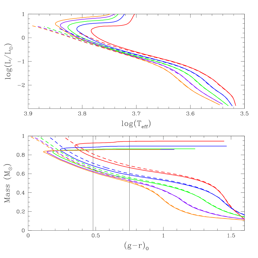
Figure 1: Comparison of the Dartmouth isochrones over the metallicity range of interest for two different ages. Red represents [Fe/H]=$-$0.5, blue $-$1.0, green $-$1.5, purple $-$2.0 and orange $-$2.5. The solid lines are 10 Gyr. isochrones and the dashed lines are 3.5 Gyr. For the main sequence range, the temperature, $(g-r)_{0}$ color, mass range, and luminosity discrepancies for the two ages are not large. Thus, we can use the younger isochrones for our modeling purposes.

Throughout this analysis, we use isochrones from the Dartmouth Stellar Evolution database to define temperature, surface gravity, and broadband $ugriz$ magnitudes for our model stars (Dotter et al., 2008). The isochrones we select cover a metallicity range from [Fe/H]=$-$0.5 to $-$2.5, with [$\alpha$/Fe]=0 for masses between 0.1 and 1.0 M_⊙ . This spread reflects the metallicity-mass range of our preliminary G-K dwarf sample from SEGUE (see § 2.3). We examine only the main sequence section of the selected isochrones. Additionally, our model atmospheres limit us to stars cooler than 8000 K. Although we expect the SEGUE stars to be around 10 Gyr in age, to simulate targets on the main sequence up to 8000 K requires using a 3.5 Gyr isochrone (see Fig.1). Even though this age is less than the expected age for these stars, there are not significant differences between the isochrones of various ages on the main sequence (see Fig.1). The Dartmouth isochrones are especially useful as they are calculated directly for $ugriz$ photometry and do not require any conversions between $UBVRI$ and SDSS photometry, which could be a potential source of uncertainty as these transformations are metallicity dependent and incomplete over our temperature and metallicity ranges. We also used the isochrones from the Padova database (Girardi et al., 2004), which cover a similar metallicity and age range. Using these two sets of isochrones provided similar numerical results, and we selected the Dartmouth isochrones for the bulk of our work as they are in uniform incremental steps of metallicity, making our distribution of models over metallicity smoother.

2.2 Binary Properties

Previous analyses of G dwarf binaries in the solar neighborhood, in particular Duquennoy & Mayor (1991), have established empirical expressions for various orbital properties, such as period and eccentricity. By utilizing these, in conjunction with different empirical descriptions of stellar mass functions, we can model a sample of binaries that mimic observed conditions. Our adopted model parameters for the synthetic pairs follows.

2.2.1 Period

We assign each pair a period between 0 and 10¹⁰ days based on the Gaussian distribution in $\log P$ from Duquennoy & Mayor (1991). This work analyzed the properties of 82 pairs with G dwarf primaries in the solar neighborhood from the CORAVEL and Gliese catalogs, empirically fitting a lognormal to the period distribution with an average $\log P=$4.8 and $\sigma_{\log P}=$2.3, where P is in days.

2.2.2 Primary Mass Distribution

We use three different distributions to define the masses of the primaries. The color range of our SEGUE G-K dwarf sample is 0.48$\leq$$(g-r)_{0}$$\leq$0.75, implying a mass range from approximately 0.5 to 0.8 M_⊙  using the Dartmouth isochrones over a range of metallicities (see Fig. 1). Our mass range extends slightly beyond the typical mass range of G and K dwarfs, going from 0.5 to 1.0 M_⊙ , to ensure that we account for all potential contaminants; higher mass primaries can be bumped into the color region of G-K dwarfs when blended with cooler secondaries. Similarly, G-K dwarf primaries can potentially be bumped out of a rigid color cut when blended with a secondary.

We use three models for the mass distribution of the primary stars from Salpeter (1955), Kroupa (2001), and Chabrier (2003). The Salpeter distribution, based upon the observed luminosity function at that time, is a simple power law:

$$f(M)\propto M^{-2.35}$$ (1)

The Kroupa (2001) model is in the form of three broken power laws over different mass ranges and is quite similar to a Salpeter distribution over the mass range of the primaries. For the primaries,

$$f(M)\propto M^{-2.3}$$ (2)

Lastly, work by Chabrier (2003) utilized observational data of the bottom of the main sequence to determine that the basic power law relationships defined by Kroupa and Salpeter are not accurate for stars below M_⊙. The Chabrier distribution for stars with M$<$M_⊙  is based on a Gaussian form:

$$f(M)\propto\exp[-(\log M-\log m_{c})/2\sigma^{2}]$$ (3)

where $m_{c}$ is the mean mass, 0.079 M_⊙ , and $\sigma$ is the variance in $\log(M/$M_⊙ $)$, 0.69. Chabrier also determines a mass function for system masses to account for unresolved binaries. This function is consistent with the single mass function with a 50% binary fraction (Chabrier, 2003). As we want the individual mass of primary and secondary, rather than their total mass, we use the individual rather than the system mass function. To ensure that not using the system mass relationship would not significantly affect our numerical results, we used it in conjunction with our Monte Carlo modeling, finding that its numerical results were within the errors of those from the standard Chabrier distribution. We normalize all three of these mass distributions according to the mass range they cover, from 0.5 to 1.0 M_⊙.

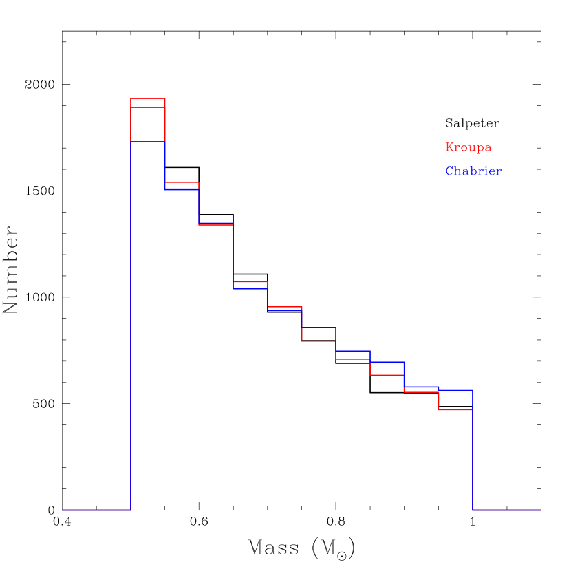
Figure 2: The three mass distributions for the primary stars. They are quite similar to one another, resulting in the primary mass distribution being largely model independent.

Despite differences in form, these three distributions are, in actuality, quite similar to one another (see Fig. 2), making it largely irrelevant which of the three we choose. When not explicitly stated, we use the Chabrier distribution, because it was defined specifically for our mass range of interest.

2.2.3 Secondary Mass Distribution

The mass distribution for the secondary depends on both the mass of the primary and the period of the system. We use primary-constrained pairing, i.e. the mass of the secondary is determined from a specified distribution and is limited by the mass of the primary (Kouwenhoven et al., 2008); more specifically, the mass of the secondary is between 0.1 M_⊙  and M_prim. The photometric uncertainties of SDSS are 2% for $gri$ and 3% for $u$ and $z$ (Ivezić et al., 2004; Abazajian et al, 2005). For our binaries, the photometric changes from blending with a secondary are significant, i.e. greater than the uncertainties, for a primary of 0.5 M_⊙  when it is blended with a 0.2 M_⊙  secondary for a change in $g$ and $r$ of $\approx$0.05$-$0.1, depending upon the metallicity. By expanding our model to secondaries with masses of 0.1 M_⊙ , we ensure that we cover the entire mass range where a companion can influence the parameters, both photometric and spectroscopic, of its primary.

Work by Abt & Willmarth (1992) on $\sim$70 binaries with F-G type primaries determined that for those with short period, defined as less than 100 years, the distribution of secondary masses is flat, confirming previous work using a sample of 94 binaries with solar-type primaries by Abt & Levy (1976). This is of particular interest, because Hurley et al. (2005) find that having a flat mass distribution for short period binaries results in more blue stragglers in their models of M67, helping them better match observations. Duquennoy & Mayor (1991), however, hesitate to adopt a flat mass distribution for short-period binaries, while acknowledging the ambiguities resulting from their small sample size of $\sim$80 pairs. Currently, there is not firm observational evidence for or against a flat secondary mass distribution for pairs with short-periods, as the sample sizes analyzed have been too small to determine the distribution conclusively, and future work must be done on much larger observed samples.

For our models of short periods, defined as less than 1000 days based on the criteria of Duquennoy & Mayor (1991), we try both a flat distribution, as determined by Abt & Willmarth (1992), and one that follows the behavior defined for long periods. We model this for all of our secondary mass distributions. Defining a flat mass distribution for short-period binaries affects approximately 22$\pm$1% of all G-K dwarf blends by moderating the secondary mass distributions. For all of the distributions, the number of low mass secondaries are decreased and the number of high mass are increased. Despite this, the basic overall shape of the distribution is not affected (see Fig. 3). It also does not affect the numerical results. The number of blended pairs, etc. are within the uncertainties of one another for simulations with and without the short-period modifications. For the remainder of this analysis, we assume that short- and long-period binaries have the same secondary mass distribution, independent of the system’s period.

We employ a variety of distributions to model the secondary masses, including those used to model the primary masses, the Salpeter, Kroupa, and Chabrier distributions. All secondary mass determinations are normalized assuming a mass range from 0.1 M_⊙  to the mass of the primary. Note that the Kroupa distribution has a different exponent at masses less than 0.5 M_⊙ :

$$f(M)\propto M^{-1.3}\textrm{ if }0.08\leq M\leq 0.5$$ (4)

Additionally, we adopt two relationships based upon q, the mass ratio between the secondary and primary. The first is a Gaussian distribution from Duquennoy & Mayor (1991):

$$f(q)\propto\exp[-(q-\mu)^{2}/2\sigma^{2}]$$ (5)

where $\mu=$0.23 and $\sigma=$0.42. The second q ratio distribution we use is from Halbwachs et al. (2003). This model takes into account the prevalence of “twins,” binaries with two stars of approximately equal mass. Similarly to Duquennoy & Mayor (1991), it is derived empirically from CORAVEL data, but covers a slightly wider range of spectral type, from F7 to K, and includes cluster stars in addition to targets in the solar neighborhood. This particular model has three peaks, at q=0.25, 0.65 and 1.

These five different models have very different distributions, as expected and shown in Fig. 4. By using all of these different methods, we can compare the results and measure the effect of using a mass function rather than an empirical q distribution to define the secondary mass distribution. We discuss this further in § 3.

2.2.4 Eccentricity

We adopt an eccentricity distribution from Duquennoy & Mayor (1991). If the period is less than the circularization period, $\approx$10 days, the orbit is circularized by tidal interactions and has an eccentricity, e, of 0. The eccentricity of tight binaries, with 10$\leq$P$\leq$1000 days, has a Gaussian distribution, with a mean of 0.31 and a dispersion of 0.155. Again, these values were determined from a sample of nearby G dwarfs; similar mean values have been determined for young open clusters and halo stars as well (Duquennoy & Mayor, 1991) . Lastly, we consider the eccentricity of long-period binaries, with P$>$1000 days. Duquennoy & Mayor (1991) determined that for these binaries,

$$f(e)\propto 2e$$ (6)

Using these three distributions, we assign an eccentricity to each sample pair based upon its period.

2.2.5 Inclination

We assume a flat distribution of $\cos I$ between 0 and 1, where I is the inclination angle. This assumes that all orientations of the binary system in space are equally likely.

2.2.6 Phase

The position of the secondary with respect to the primary determines whether or not the two will be blended within the SDSS PSF. For each secondary we pick a random mean anomaly, M, between $-\pi$ and $\pi$. Combining this with the assigned eccentricity, we calculate the eccentric anomaly, EA, using iterations of a Taylor series expansion of the Kepler equation (Murray & Dermott, 2000).

$$f(EA)=EA-e\sin(EA)-M$$ (7)

This results in each pair having an EA between 0 and 2$\pi$. For pairs with non-negligible eccentricities, the secondary will spend a larger fraction of its time in orbit far away from the primary. Determining the parameter EA from M takes this distribution into account. From the eccentric anomaly, we then calculate the true anomaly, F.

$$\tan(F/2)=\sqrt{\frac{1+e}{1-e}}\tan(EA/2)$$ (8)

With F, we determine r, the distance between the two stars at that particular orbital phase.

$$r=\frac{a(1-e^{2})}{(1+e\cos(F))}$$ (9)

where a is the semimajor axis of the orbit, which we derive from the period and masses of the pair. Finally, we select random values between 0 and 2$\pi$ for $\Omega$, the longitude of the ascending node, and $\omega$, the argument of pericenter. We use r in conjunction with the true anomaly, F, $\Omega$, and $\omega$ to determine the two orthogonal components of the projected distance between the secondary and the primary, $X$ and $Y$.

$$X = r[\cos\Omega\cos(\omega+F)-\sin\Omega\sin(\omega+F)\cos I]$$ (10)

$$Y = r[\sin\Omega\cos(\omega+F)+\cos\Omega\sin(\omega+F)\cos I]$$ (11)

Using $X$ and $Y$, we then calculate the projected magnitude of the separation on the sky of the two stars, R:

$$R=\sqrt{X^{2}+Y^{2}}$$ (12)

2.3 Photometric Blending

As mentioned earlier, for a pair to be blended photometrically, they must be within 1.4″  of each other on the sky. Combining the orbit information with an assigned distance, we can determine whether or not the pair fulfill the separation criteria. If blended, we then combine $ugriz$ magnitudes, based on isochrones.

To model the distances to each pair, we determine an empirical distance distribution for G and K dwarfs with spectra from SEGUE using their target selection parameters in the $(g-r)_{0}$ color and $r_{0}$ magnitude (Adelman-McCarthy et al., 2008). From this sample, we first eliminate all targets for which the SSPP was unable to determine a metallicity, temperature, or $\log\,g$. In total we extract approximately 20,000 G-K stars from SEGUE, two-thirds of which are SEGUE-defined G type.

For each SDSS target, we then select a 10 Gyr comparison isochrone from the Dartmouth set based upon the SSPP metallicity over a range of [Fe/H]=$-$0.5 to $-$2.5 (see § 2.1 for more information on the isochrone selection). If the target’s metallicity falls between two isochrones, we interpolate. We then match the target to the isochrone by SSPP temperature and pull out the modeled ugriz magnitudes, surface gravity, and mass from the isochrone. Comparing the isochrone magnitudes to those detected by SDSS, we use the distance modulus to determine an approximate distance to each target based on the $g_{0}$ and $r_{0}$ magnitudes, weighted equally. For this sample we find a range of distances from 0.5 to 6 kpc (see Fig. 5). As G dwarfs are brighter than K dwarfs, SDSS can observe them at greater distances. Based on the magnitude limits of SDSS, we select a distance range from $\sim$750 and $\sim$3700 pc. to ensure that our G and K dwarf sample occupy the same volume of space. We fit the distribution of distances in this range using a linear least squares fit, measuring:

$$f(d)=-298(d/kpc)+1027$$ (13)

Each modeled pair is thus assigned a distance according to this distribution, and, in conjunction with each pair’s R value, we derive a projected separation on the sky in arcseconds.

If our sample of dwarfs from SEGUE is contaminated by binaries, the distance distribution will be affected; targets will appear brighter, and we will underestimate their distance. To simulate this effect, we adjust our measured distances for the G-K dwarfs in SEGUE. We select a random 65%  of our sample, the percent expected to be in binaries (Duquennoy & Mayor, 1991), and double their calculated distance. As undetected secondaries will cover a range of masses, by assuming that all of the pairs are twins, we calculate the most extreme scenario of binary distance contamination. We again determine a linear least squares fit to the distribution of distances, which now has a much shallower slope:

$$f(d)=-128(d/kpc)+625$$ (14)

For the G-K color pairs, using the most extreme contaminated distance relationship results in an additional $\sim$2 percentage points of blends, independent of metallicity and mass distributions. Consequently, we feel confident using the original distance relationship and ignoring the potential binary contamination effects.

2.4 Spectroscopic Blending

We have determined the combined magnitudes of pairs photometrically blended in SDSS photometry. However, as the spectroscopic fiber for SEGUE is 3″, we must take into account that there are some pairs that, although not photometrically blended, are spectroscopically blended.

Spectroscopic blends are photometrically distinguishable. If SEGUE recognizes them as close pairs and systematically avoids them, due to concerns about spectral contamination, we do not need to take spectroscopic blends into account. The SDSS photometry pipeline has a deblending function capable of resolving a binary with a separation of 1″  or greater (Yanny, private communication). If the deblend is not done well, as indicated by certain photometric flags, SEGUE avoids that particular target. However, a well-resolved pair will not be avoided by SEGUE. As SDSS can separate stars as close as $\sim$1″, this indicates that SEGUE will likely include many binaries with separation less than 3″  in the sample, and the primaries will have their spectroscopic parameters contaminated by a secondary. Thus, we count every pair with 1.4″$\leq r\leq$3″  as a spectroscopic blend capable of contaminating the SEGUE sample and affecting SSPP measurements.

3 Number Comparison

We use a Monte Carlo method to determine the effect of binaries on the G-K spectroscopic sample in SEGUE. The first step is to determine how frequently a photometric blend will cause a binary that would otherwise fall into the G-K sample to fall outside the color range, or how often a photometric blend will put a pair into the sample whose primary would otherwise be too blue. We examine whether the fraction that shift into or out of the color range depends on the primary or secondary mass function. For each combination of metallicity and mass distributions, we pick 100,000 primaries drawn from the primary mass distribution and match them with 100,000 secondaries, drawn from the secondary mass distribution. These pairs are given orbits in accordance with the previous discussion (see § 2.2). As shown in Fig. 2, the three different mass distributions for the primaries result in approximately the same number of stars at each mass. However, the mass distributions for the secondaries have very different forms (see Fig. 4). For each combination of primary and secondary mass distribution, we determine the number of pairs that are photometrically (projected closer than 1.4″) and spectroscopically (projected closer than 3″) blended.

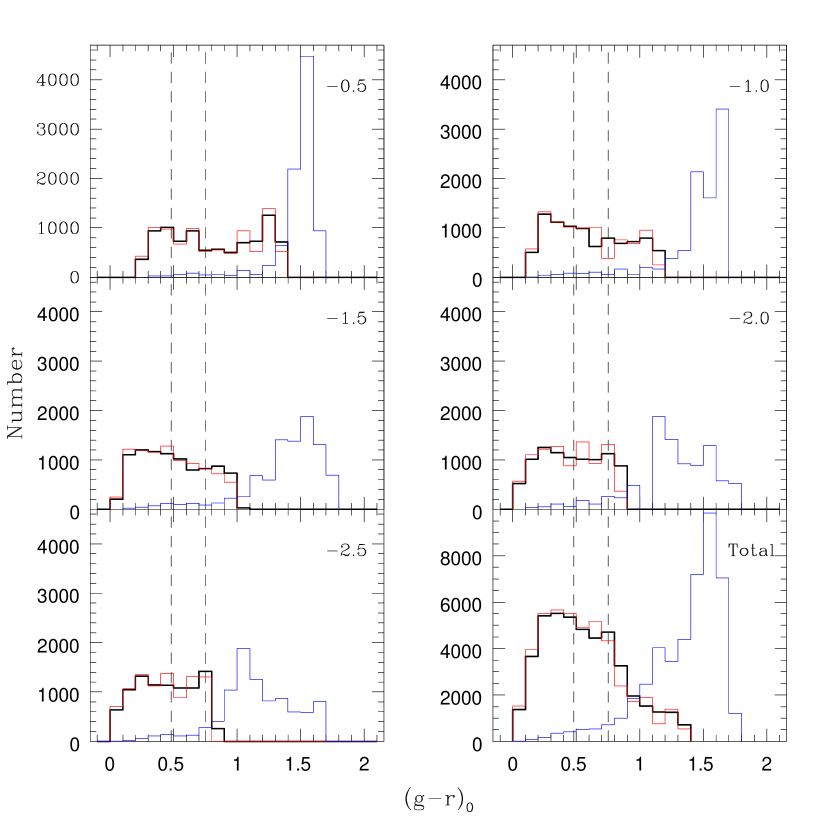
Figure 6: Histograms of the shift in $(g-r)_{0}$ color over the entire blended sample. The red histogram represents the primaries, the blue is the secondaries and the black is the binaries. The dashed lines indicate the G-K dwarf color cut as specified by SEGUE target selection (Yanny et al., 2009). At the top right corner of each plot is the metallicity for that sample; the distributions shift slightly with metallicity. The combined sample is in the bottom right plot. Note that the numbers of targets in the color cut range does not vary significantly from the primaries to the pairs, indicating that the addition of a secondary will not have a large affect on the population numbers in the G-K range. This model assumes a Chabrier primary and secondary mass distribution, although the behavior is similar for the range of mass distributions.

Of a sample of 100,000 pairs, approximately 90$\pm$1% are photometrically blended, regardless of mass distribution or metallicity. Approximately 40% of all targets will have their $(g-r)_{0}$ color shifted by an amount greater than the uncertainties in SDSS photometry by the addition of a secondary. We then use color cuts to extract the pairs that will be within the $(g-r)_{0}$ color range of G and K dwarfs. These are the binaries that will be contaminating the G-K dwarf sample and possibly affecting SEGUE target selection, resulting in potential errors in studies of stellar populations. Similar to the larger sample, $\approx$40% of the G-K dwarf sample will have their $(g-r)_{0}$ color shifted by more than the SDSS photometric uncertainty. In Fig. 6, we compare the $(g-r)_{0}$ color distribution for the primaries to that of the blended pairs over a range of metallicities, examining the numbers of targets that remain within the G-K dwarf color cut. On average, 30$\pm$2% of the 100,000 primaries are within the G-K color cut, compared to 28$\pm$2% of the pairs (see Table 1). The addition of a secondary bumps out slightly more targets from the G-K range than it bumps in. On average, 2% of the 100,000 primaries will be bumped into the color cut by adding in a secondary; 3% will be pushed out of the $(g-r)_{0}$ range by a companion. In addition to calculating percentages, we examine the most frequent color shifts by comparing the $(g-r)_{0}$ of the blended binaries to those of the primaries. We analyze a sample which includes every combination of primary and secondary mass distribution at every metallicity. For the entire sample, the addition of a secondary most often shifts $(g-r)_{0}$ by 0.01 with $\sigma$=0.02. When we extract all of the targets for which the primary is in the G-K dwarf SEGUE color range, the shift and $\sigma$ are the same. The population error resulting from photometric binary contamination in target selection is minimal, as the shifts themselves are small.

We isolate G-K dwarf spectroscopic blends by selecting pairs where the primary is within the color cuts. As noted earlier (see § 2), using 3″  as the criteria is the most extreme scenario for spectroscopic contamination. On average, about 3% of the G-K sample are spectroscopically, but not photometrically, blended. Thus, even for the largest possible chance of purely spectroscopic contamination, the likelihood is negligible.

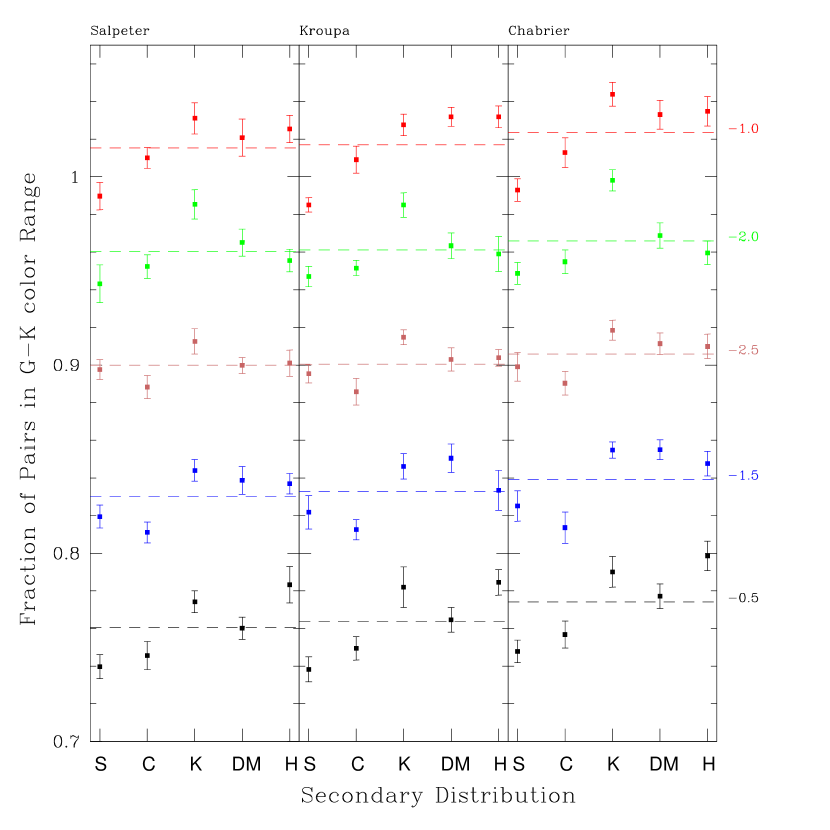
Figure 7: The fraction of pairs that are blended spectroscopically and photometrically in the sample of G-K range binaries. The three panels represent the three different mass distributions of the primaries, Salpeter, Kroupa, and Chabrier. The x axis is labeled with the various mass distributions of the secondaries: Salpeter (S), Chabrier (C), Kroupa (K), Duquennoy & Mayor $q$ ratio (DM), and Halbwachs $q$ ratio (H). Each color represents a different metallicity. Black is [Fe/H]=$-$0.5, red is $-$1.0, blue is $-$1.5, green is $-$2.0, and pink is $-$2.5. Each combination of primary and secondary mass distributions was run 10 times; the error bars reflect the RMS variation in the blended fraction for the total 100,000 target sample. The average fraction for all of the secondary distributions is noted with the dashed line. As expected, the fractions for the Salpeter and Kroupa primary mass distributions agree, while the Chabrier is slightly different. Additionally, all but a few of the fractions for each of the secondary distributions agree with one another within the RMS uncertainties, indicating that the fraction of blended binaries is approximately independent of the secondary mass distribution.

In Fig. 7, we plot the fraction of blended pairs within the G-K dwarf color range, both photometric and spectroscopic, versus the secondary mass distributions for all three primary distributions over the range of metallicities. As listed in Table 1, we examine how many primaries are initially in the G-K color range and compare it to the number of pairs within the color cut. We plot the average blend number with the error bars representing the standard deviation among the 10 samples of 10,000. As expected, there is variation in the blended fraction related to the different secondary distributions. However, in general, the statistics for the range of secondary distributions agree with one another within uncertainties for each primary mass distribution, indicating that there is not a substantial numerical difference from one model to another (see Table 1). We are not surprised by this because different factors, such as the short period flattening and Chabrier system mass distribution, appeared to have little to no effect on the number of resulting blends as well. The fractions determined for the Salpeter and Kroupa primary distributions are quite similar to one another, whereas the Chabrier results are slightly increased.

Recent work by Metchev & Hillenbrand (2009) determined that the mass functions of companions are different than those of individual objects, making it inaccurate to use the empirical mass functions, such as the Salpeter, Kroupa, and Chabrier relationships, to model and analyze stellar secondaries. However, Metchev & Hillenbrand (2009) find good agreement between the distribution of companion masses and the relationship measured by Duquennoy & Mayor (1991) for all targets with q$>$0.1. We do not find significant variation in our blended G-K fraction with different secondary models. The model using the q relationship from Duquennoy & Mayor (1991) appears quite similar numerically to the other models, where we pull random secondary masses from an IMF. Thus, we are not particularly concerned about the detected differences between the primary and secondary mass function, as it does not appear to have a significant effect on our statistical modeling.

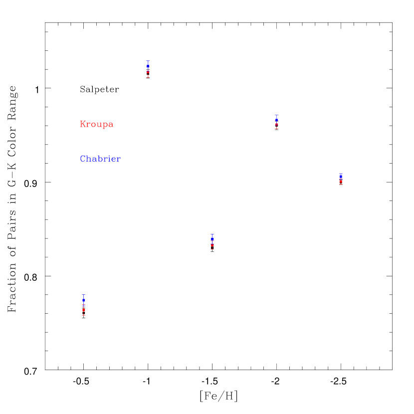
Figure 8: The average fraction of blended pairs for each metallicity. The black points have a Salpeter primary mass distribution, the red have Kroupa, and the blue represent Chabrier. There is no particular trend of fraction of blends with metallicity; the differences are the result of our modeling scheme (see § 3). Note that the fraction of blends agrees quite well for Salpeter and Kroupa but is slightly different for Chabrier, which is slightly higher, as we saw in Fig. 7. The uncertainties are the RMS variation for the average fractions designated by the dashed lines in Fig. 7 determined from the complete sample.

For each primary distribution, we plot the average fraction of blends at each metallicity and compare them in Fig. 8. There is no clear relationship between the blended fraction and metallicity. The fractional variation over our metallicity range is likely due to our color cut, rather than a real physical effect. At each metallicity, the mass range of our pairs covers a different $(g-r)_{0}$ color range. Lower metallicity primaries cover a smaller range of colors which are shifted more towards the blue. Conversely, the spread in $(g-r)_{0}$ color range of the secondaries is larger for lower metallicities. The different spread of colors in both primaries and secondaries changes the effect a secondary has on the primary’s color, in particular whether or not it can shift primaries in and out of the G-K color range. This causes variation, but not a consistent trend, in the fraction of blends that remain within the G-K color range with metallicity. Independent of the effects of metallicity, all of the blended fractions determined by the different distributions agree with one another within the errors, indicating that our choice of mass distributions has little effect on our numerical results.

4 Spectroscopic Modeling

To understand the effect of simulated binary contaminants on SSPP parameter determinations, we spectroscopically model a grid of binaries over the range of metallicities and process them through the pipeline. Each member is of a particular mass, with the temperature, surface gravity, luminosity, and ugriz magnitudes extracted from the Dartmouth isochrones. We then model the spectra using a MARCS model atmosphere grid (Gustaffson et al., 2008) in conjunction with the TurboSpectrum program using these Dartmouth parameters (Alvarez & Plez, 1998).

4.1 Model Atmosphere Grid

We utilize MARCS model atmospheres of standard chemical composition and plane parallel geometry to develop a grid of model spectra, covering a range of temperature, surface gravity, and metallicity (Gustaffson et al., 2008). Each spectrum in the grid is interpolated from MARCS model atmospheres using the bracketing values in effective temperature, surface gravity, and metallicity. For our interpolation, the temperature is in increments of 25 K from 3200 to 8000, $\log g$ in 0.1 dex from 3.0 to 5.5, and metallicity in steps of 0.5 ranging from [Fe/H]=$-0.5$ to $-2.5$. For standard composition models of [Fe/H]=$-0.5$, [$\alpha$/Fe] is defined as 0.20. For all other metallicities, [$\alpha$/Fe]=0.40. Finally, our microturbulence is defined as 2 km/s.

4.2 Model Synthesis

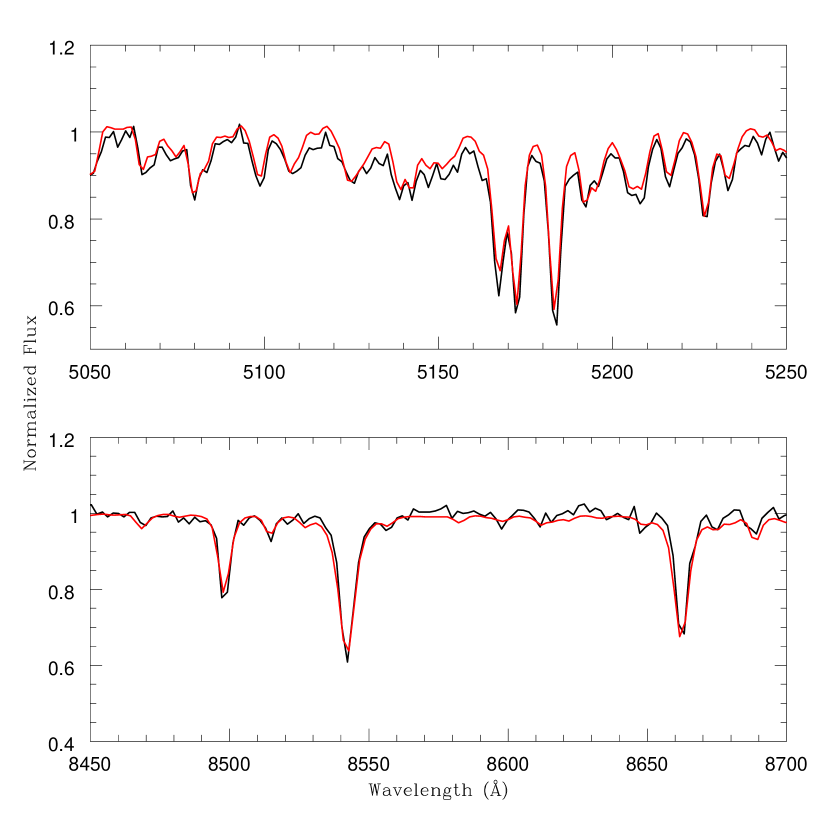
Figure 9: A processed model spectrum (red) vs. an actual SEGUE spectra (black). We have focused in on two regions for comparison: the region of MgH features (top) and the Ca II triplet region (bottom). Both are important for determining parameters in the SSPP. The model spectra has been made with TurboSpectrum from a grid of MARCS model atmospheres. The model is then adjusted to match the dispersion of SDSS and binned to have 69 km/s per pixel. Note that both of these spectra have been normalized using SPECTRE continuum division to make them easier to compare. The parameters of the model are determined from Dartmouth isochrones. This particular model has a temperature of 5600 K, $\log g$ of 4.6, and [Fe/H] equal to $-$0.5. It represents a 0.8 M_⊙  star. This SEGUE target has a temperature of 5612 K, a $\log g$ of 4.5, and [Fe/H] of $-$0.59 according to the SSPP.

For each metallicity, we synthesize 10 model stellar spectra, corresponding to the masses from 0.1 to 1.0 M_⊙  by interpolating a MARCS model atmosphere and processing it in TurboSpectrum (see Table 2). These models cover the same wavelength range as SEGUE, 3800-9200Å, in 0.1Å  increments. To simulate the spectra of binaries, each primary spectra, from 0.5 to 1.0 M_⊙ , is combined with all secondaries of lesser or equal mass. TurboSpectrum provides us with the flux from the star; combining this with the radii of the stars squared, as determined from the Dartmouth isochrones, we calculate the luminosity of each star. The ratio of these luminosities determines how much an undetected secondary will affect its primary. We then apply an SDSS dispersion file to Gaussian-smooth the synthetic spectra to model the instrument output. Lastly, the synthetic spectra are binned into pixels of width 69 km/s. These modifications ensure both that our spectra are accurate reflections of data taken by SEGUE, and that our models can easily be run through the SSPP. We have compared a synthesized model and a SEGUE spectrum in Fig. 9.

5 Parameter Shifts

We do not expect our synthetic spectra to be a perfect match to real spectra, particularly for the strongest features, such as the Balmer lines, because we do not take into account known difficulties related to NLTE, 3-D, and chromospheric effects in our models. Therefore, we are not surprised that there are differences between the parameters we use to model the spectra and the parameters that the SSPP derives. The critical issue is understanding how much simulated binarity changes the values the SSPP determines for the atmospheric parameters of our sample of synthetic binaries, independent of modeling errors.

We run our synthetic spectra of single stars with 0.5 M_⊙ $\leq$M$\leq$1 M_⊙  through the SSPP as a control sample to determine the SSPP parameter offsets for temperature, metallicity, surface gravity, and $\alpha$-enhancement. The values measured for the control group of primaries are listed in Table 3. The temperatures determined by the SSPP for this sample most frequently overestimate the model temperature by around 12 K (see Fig. 10), a negligible amount with respect to the expected errors ($\sigma(T_{eff})$$<$150 K) for the pipeline (Lee et al., 2008a). We also compare the [Fe/H] value determined by the pipeline to that set for the models (see Fig. 11). The pipeline overestimates the metallicity of the sample with a mode of $\sim$0.15 dex, less than the expected error of $\sigma([Fe/H])$=0.24 dex (Lee et al., 2008a). Whereas temperature and metallicity are overestimated by the pipeline, surface gravity is underestimated (see Fig. 12). The most common shift is a decrease of $\sim$0.25 dex, which is comparable to the expected SSPP error of 0.29 dex. Lastly, we examine the offsets in [$\alpha$/Fe] in Fig. 13. All of the synthetic spectra have [$\alpha$/Fe] set to 0.2 or 0.4, based on the MARCS model atmosphere metallicity. When processed, the SSPP finds a wide range of $\alpha$-enhancement, spreading the values over a range from $\sim$$-$0.5 to $\sim$0.25. The most frequent offset is $-$0.075 dex. Since the offsets are smaller than or on the order of the SSPP errors, we find that our model spectra are more than adequate for measuring the effects of binary contamination.

Using this control sample of primaries, we define a temperature, metallicity, and surface gravity offset between the models and the SSPP parameters due to assumptions in our model synthesis. We then compare the values determined for the grid of binaries with those determined for the primary member of each pair. The parameters SSPP determines for each pair are listed in Table 4, and the differences between these values and those determined for the primary control group are in Table 5. In general, for all of the parameters, temperature, metallicity, surface gravity, and alpha enhancement, the shifts between the SSPP determinations for the primaries and the pairs are most often within the expected SSPP uncertainties (see Fig. 14, Table 5). There is a slight anticorrelation between these values for the [$\alpha$/Fe] with a slope of $-$0.56, but otherwise the relationships are flat.

We also compare the shifts for the grid of pairs to those for the primaries to see if there is any correlation between the two (see Fig. 15). There appears to be small anticorrelations, all less than a slope of $-$0.6, between the amount a primary is shifted and the amount a pair is shifted, determined by performing linear least squares fits on the points. These anticorrelations are small, indicating that the addition of a secondary shifts the SSPP determinations independently of the standard offsets. The largest anticorrelation is $-$0.57 for the [$\alpha$/Fe] measurements.

For the following analyses, we examine the shifts in atmospheric parameters due to an undetected secondary in two ways. First, we examine the “grid” of synthetic spectra. Namely, we calculate the differences between the synthetic binaries and their associated primaries individually for every modeled spectra. Second, we examine the shifts of a numerical population model of stars. The Galaxy does not have a flat mass distribution for stars. To accurately determine the actual shifts due to undetected binarity in our SEGUE G-K sample, we combine our numerical population modeling with our grid of synthetic spectra atmospheric parameters. We create a large sample including every combination of primary and secondary mass distributions at every metallicity as a model of the actual stellar sample. By matching each primary and secondary in this sample with the parameters in the synthetic spectra grid, we determine the most frequent shifts in temperature, metallicity and surface gravity, in addition to the spread in these shifts for a realization of the SEGUE G-K sample. We combine the numerical sample of primaries with the grid of primaries vs. model parameters to determine the uncertainties stemming from the imperfections in our synthetic spectra and the SSPP’s analysis of them. This checks the SSPP measurements for a set of known inputs, allowing us to calculate constant offsets associated with the uncertainties in the modeling. We then determine the differences between the sample of binaries and primaries. Analyzing the uncertainties from the primaries with those for the binaries, we can isolate the uncertainties that stem exclusively from binarity.

5.1 Effective Temperature

The SSPP has temperature errors of 150 K at $S/N\geq$50 (Lee et al., 2008a). The addition of a secondary decreases the SSPP measured temperature from that determined for the primary alone (see Fig. 14, 16). This is expected, as we can see by examining the changes in $(g-r)_{0}$ color (see Fig. 6). Whereas shifts in the other atmospheric parameters may be due to random errors produced by the contribution of a secondary, the downward shift in temperature is a systematic shift due to the low mass secondaries being redder than the primaries.

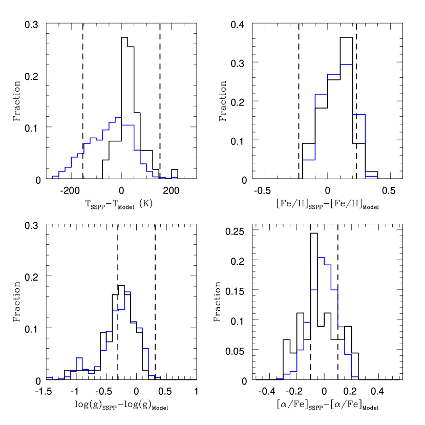
Figure 16: The offsets between the pipeline determinations for all of the modeled primaries and pairs for various SSPP parameters. The black histogram is the control group of primaries and the blue is the blended binaries. The dashed lines represent the SSPP errors for different determinations. The top left figure is for temperature, with a pipeline error of $\pm$150 K. In general, the offsets for both the primaries and pairs are well within the uncertainties of the pipeline. The top right is a comparison of [Fe/H] determinations. Similarly, most of the shifts remain within the expected errors of 0.24 dex. The bottom left is the surface gravity offsets, with an error of 0.29 dex. Many of these are shifted out of the error range. Lastly, the bottom right figure is for [$\alpha$/Fe] measurements using errors of 0.1 dex (Lee et al. in prep). For all but temperature the shape of the offset histograms are quite similar for the pairs and primaries, indicating that the addition of a secondary has little effect on the SSPP determinations for metallicity, surface gravity, and alpha enhancement. As expected, the secondary does noticeably affect the temperature determinations, systematically shifting them to cooler values.

The most frequent offset between the pair and the model temperature of the primary for the grid is approximately -12.5 K, whereas it is $\sim$12.5 K for the primary control group (see Fig. 16). The most extreme shift in the G-K color range results from a 1 M_⊙  primary with [Fe/H]=$-$2.5 with a 0.85 M_⊙  secondary shifted in temperature by 410 K. When we examine our numerical population sample of primaries, we find that the mode shift is 55 K with $\sigma(T)$ of 36 K for the largest $S/N$ (see Table 7). This indicates the uncertainty from imperfections in our synthetic spectra is $\pm$36 K.

We then use our grid of synthetic spectra to examine the mode and uncertainty in our binaries when compared to their associated primaries. First, we examine the variation in the shifts at different metallicities. Fig. 17 displays the sizes of the shifts in temperature for all targets within the G-K color cut in a 10,000 target sample at each metallicity, and finally, for all of these samples combined. There is some variation in the size and range of the shifts at different metallicities. Additionally, there is some variation in the shifts from different combinations of primary and secondary mass functions. Table 6 lists the absolute value of the shifts in temperature between binaries and primaries for spectra of infinite $S/N$; the listed uncertainties reflect the variation in these percentages from the different combinations of primary and secondary mass functions. The uncertainties listed for the “Total” sample account for variation in both mass functions and metallicity. 52$\pm$10% of the sample have the addition of a secondary shift their temperature from that of the primary by $\leq$60 K, a minimal effect (see Table 6). In fact, $\sim$82$\pm$7% of the pairs are within 150 K of their associated primary. Only $\sim$18% of the shifted pairs lie outside the SSPP temperature uncertainties at the highest $S/N$.

Our “Total” sample is our complete numerical population model, including every combination of primary and secondary mass functions at each metallicity. We use this sample to determine the effects of binarity on our SEGUE sample. Examining the mode and $\sigma(T)$ shows that the binary sample is most frequently shifted down 15 K in temperature, with a variance of $\pm$72 K (see Fig. 18, Table 7). This variance represents the uncertainty from both binarity and the synthetic modeling errors, which we measured above to be $\pm$36 K. We can isolate the uncertainty from undetected secondaries using the values determined for the primaries vs. the model parameters, assuming the errors add in quadrature. For infinite $S/N$, there is a systematic shift of $-$15 K and an additional uncertainty of $\pm$62 K due to undetected binaries.

5.2 Metallicity

The metallicity determinations are relatively unaffected by the addition of a secondary. The primary control group most often overestimates the metallicity by $\sim$0.15 dex (see Fig. 11). Whereas the addition of a secondary affected the shifts in temperature, there is little shift in the metallicity determinations of pairs versus primaries (see Fig. 16). The largest metallicity shift for targets in the $(g-r)_{0}$ color cut range defined for G and K dwarfs is 0.36 dex. This shift is for a pair of metallicity $-$0.5, a 0.75 M_⊙  primary with a 0.6 M_⊙  secondary.

Once again, we combine the shifts in the grid of synthetic spectra with the numerical modeling to determine the metallicity uncertainties most often found in a SEGUE sample of G-K dwarfs (see Fig. 19). Similar to the temperature shifts, there is variation in the metallicity shift over the range of [Fe/H]. There is little variation with different combinations of primary and secondary mass distributions (see the uncertainties listed in Table 8). For the blended pairs with infinite $S/N$, $\sim$62$\pm$3% will be within 0.05 dex of the determination of the primary; the addition of a secondary does not have a significant effect (see Table 8). While $\sim$18% of the shifts in temperature are outside the SSPP uncertainties, only $\sim$1% of the binary sample are shifted by an amount greater than $\sigma([Fe/H])$ from the SSPP for the infinite $S/N$ sample.

We expect the metallicity determinations of the pipeline to agree as well if not better than temperature measurements, as both stars in the pair are of the same metallicity. This is reflected in the mode and $\sigma([Fe/H])$ determined for the large unbiased sample (see Fig. 18 and Table 7). Using the same methodology as in § 5.1, we find that a sample of G-K dwarf stars at infinite $S/N$ will have no systematic shift but an additional uncertainty of around $\pm$0.05 dex.

5.3 Surface Gravity

We next consider the surface gravity determinations of the pipeline. The control group of primaries is shifted down in surface gravity (see Fig. 12), with a mode of $-$0.25 dex, within the expected error of 0.29 dex (Lee et al., 2008b). The addition of a secondary does not significantly affect the surface gravity offsets for the grid of synthetic spectra, as shown in Fig. 16, shifting the mode to 0.15 dex.

Again, we apply the grid of synthetic values to our unbiased numerical sample (see Fig. 18). Using the same methods used for temperature and metallicity, we find that the uncertainty from binarity for the G-K dwarf sample is around $\pm$0.25 dex (see Table 7). At different signal-to-noise ratios, the uncertainties in the primary sample are similar or larger than those of the binaries. This implies that the effects of an undetected secondary are minimal for measurements of $\log g$ in the SSPP.

5.4 [$\alpha$/Fe]

Each of the models has a specified [$\alpha$/Fe] value defined by the properties of the MARCS model atmospheres’ metallicity and composition model. As we are using the standard composition models, for [Fe/H]=$-$0.5, [$\alpha$/Fe] is set to 0.20. For all our other metallicities, [$\alpha$/Fe]=0.40. We compare the control group of primaries to the [$\alpha$/Fe] determined by the SSPP in Fig. 13. The spread of measurements for the grid of synthetic primaries is large, with a mode of -0.075 dex and a range from approximately $-$0.3 to 0.3. The addition of a synthetic secondary shifts the mode to -0.025 with a spread of shifts that looks more Gaussian for the grid of binaries (see Fig. 16). A KS test indicates that the distributions have a 60% chance of being from the same parent sample.

Because we are spectroscopically blending pairs of the same metallicity and composition (i.e. the primary and secondary have the same [$\alpha$/Fe] values), we expect there to be little difference between the parameters determined for the primaries and the blended binaries. When we apply our grid of differences to the unbiased sample, we calculate an uncertainty from binarity of around $\pm$0.10 dex (see Table 7). However the uncertainties in the primary sample are comparable in size to those of the binaries, indicating that binarity is not a dominant uncertainty for measurements of [$\alpha$/Fe].

5.5 Effects of the Signal-to-Noise Ratio

It is possible that signal-to-noise ratio effects can diminish the effect of a secondary. In particular, noise in the spectrum could overwhelm any contributions from an undetected companion. We analyze both the original infinite signal-to-noise synthetic spectra and also degrade each model to a median signal-to-noise ($S/N$) of approximately 50, 25 and 10, covering the $S/N$ range of SEGUE’s targets. A model of the noise in SEGUE has been applied to high $S/N$ stellar spectra over a range of spectral types to simulate spectra with signal-to-noise ratios from 6 to 60 (C. Rockosi, private communication). Using these realizations, we calculate the $S/N$ at each point in the spectrum. As the noise patterns can potentially vary with spectral type, we match up the SEGUE $S/N$ models to our synthetic spectra based on $(g-r)_{0}$ color. We then compute a value for the noise fluctuation at each point in our model spectra based on the $S/N$ of the noise-modeled spectra. We convolve this noise value with a Gaussian, and add it to our spectra signal-to-noise ratios of 50, 25, and 10.

We run the degraded and infinite $S/N$ models of the control sample of primaries and modeled binaries through the SSPP. To isolate the effect an undetected secondary has on the parameter determination of the SSPP, we compare the primary and pair values for each model at each $S/N$ (see Fig. 20). We determine the difference between the primary and pair values and compare these to the variance of the parameter in the control group, isolating the effect of a blended secondary at different $S/N$. As expected, as the $S/N$ decreases, the spread determined for all atmospheric parameters increases. For $S/N>$10, the distributions are quite similar, showing similar effects of binarity from a signal-to-noise of $\sim$100 to 25. For $S/N$ of 10, the spread of values increases greatly. With spectra this noisy, the SSPP accuracy is already decreased significantly. With the spectral contribution of an undetected secondary, it is even more difficult for the SSPP to determine accurate atmospheric parameters.

Combining our numerical and synthetic spectra modeling at a range of $S/N$, we have determined the amount of shifting in temperature and metallicity for the confidence intervals, 68%, 95%, and 99% of our modeled SEGUE sample (see Table 9). Similar to Fig. 20, this table indicates that the distributions of atmospheric parameter shifts are similar up until a $S/N$ of 10. Starting with the 1$\sigma$ interval, 68% of the sample for the entire range of $S/N$ is within $\sim$140 K, within the $S/N$=50 uncertainty of 150 K for the SSPP. Moving out to the 2$\sigma$ sample, 95% of the modeled sample of $S/N=\infty$, 50, and 25 are within 230 K. However, 95% of the modeled sample with $S/N=$10 are within 480 K, a much greater number. This behavior is also seen for metallicity. Similarly, we examined the mode and RMS of the shift for the various median signal-to-noise ratios. The uncertainties for the various atmospheric parameters tend to increase as the signal-to-noise decreases (see Table 7). This pattern continues when we isolate the uncertainty of binarity alone from the uncertainty from the synthetic spectra.

6 Conclusions

In this analysis, we have modeled samples of 100,000 binaries with primaries from 0.5 to 1.0 M_⊙  and a variation of mass distributions and metallicity, to better understand their effect as potential contaminants of the SEGUE sample in the G-K dwarf range. Work by Duquennoy & Mayor (1991) established that around 65% of F-G type stars have at least one companion. Thus, understanding how undetected binaries affect the atmospheric parameter determinations in SEGUE is crucial.

From our Monte Carlo analysis, we have determined that of a sample of 100,000 binaries, modeled using a range of mass distributions, on average 90$\pm$1% will appear spectroscopically or photometrically blended in the SEGUE sample, i.e. the two stars will be within 3″  of each other projected on the sky. Of all the pairs with G-K type primaries, approximately 30$\pm$2% of the sample of 100,000 binaries based on a $(g-r)_{0}$ color cut, $\sim$93% are blended.

To quantify the effect of an undetected secondary on the stellar atmospheric parameters T_eff, [Fe/H], and $\log g$ determined for the SEGUE spectra, we utilized a grid of synthetic spectra processed by the SSPP. We quantified the systematic offsets between the synthetic spectra parameters and those measured by the SSPP, which result from the various approximations made in our spectral modeling. We then compared the determinations for the blended pairs to those of the primaries to quantify the effect of an undetected companion. Examining the distribution of offsets at infinite $S/N$ shows that the majority of the G-K sample is within the established SSPP errors for both temperature and metallicity (see Table 6,  8). In particular, 82$\pm$7% of blended pairs with a G-K dwarf primary with $S/N$ of $\sim$50 are within the SSPP’s error of 150 K in temperature. For determinations of [Fe/H], 99$\pm$1% of these pairs have a measured metallicity that differs from that of the primary by less than the established SSPP metallicity error of 0.24 dex. Examining the modeled pairs, we find that very few are outliers in both temperature and metallicity. Of the 53 synthesized pair spectra in the G-K color range that are outliers in temperature or metallicity, only 3 are outliers in both estimates. Thus, we can assume that all outliers in metallicity are independent of those in temperature, for a total of $\sim$18$\pm$7% of the G-K blended targets shifted a significant amount in metallicity or temperature by an undetected secondary.

A search of SEGUE using CasJobs and based on the target selection parameters extracted a data set of $\sim$20,000 G-K type dwarfs in the sample. According to statistics from Duquennoy & Mayor (1991), 13,000 of these are in binaries. Applying our numerical results, we conservatively assume that 93% of these G-K binaries are blended pairs. Thus, of a sample of 20,000 G-K stars, $\sim$12,000, or 60%, are potentially affected in SEGUE by a secondary companion. Using our spectroscopic analysis, we can determine how many of this subsample are expected to have inaccurate SSPP parameter determinations, due to their undetected companion. We determined that 18$\pm$1% of the G-K blends are shifted beyond the expected uncertainties in temperature and/or metallicity in the SSPP by the presence of a secondary, a total of $\sim$2000 SEGUE targets. Thus, 11$\pm$2% of the entire G-K dwarf sample of high signal-to-noise will be significantly affected by an undetected companion in its SSPP temperature or metallicity determination. This 11$\pm$2% sample will be systematically shifted to cooler temperatures, and generally shifted down in metallicity as well. The percentage affected is similar for a $S/N$ of 50. For signal-to-noise of 25, the expected SSPP uncertainties increase (Lee et al., 2008a); $\sim$10% are shifted outside the expected uncertainties, similar to the value for $S/N$ of 50 and higher. This percentage increases significantly for $S/N$ of 10. $\sim$40% of the G-K dwarf sample will be shifted outside the expected uncertainties in temperature and/or metallicity at this signal-to-noise.

Beyond examining the percentage of targets pushed beyond the SSPP uncertainties in various atmospheric parameters, we quantify the uncertainties from our synthetic spectra individually and from the undetected secondary. Both the systematic shift and additional spread in each parameter must be taken into account when accounting for binary contamination in the SEGUE sample. The most frequent shift and spread values we derive for each $S/N$ we model are summarized in Table 7. For $\log g$ and [$\alpha$/Fe] the most frequent shifts are very small. The uncertainties in these parameters for the primary and binary samples are similar in size. Sometimes the uncertainty measured for the primary sample is even larger than that of the secondaries. The small shifts and variation in the $\sigma$ indicates that, for these two parameters, the uncertainties due to binarity are minimal with respect to the general uncertainties in determining the values themselves. For temperature and metallicity however, binarity can increase the SSPP uncertainties in a well defined way, with it systematically decreasing the measured temperature and slightly affecting the measured [Fe/H]. Additionally, the shifts in metallicity are quite small, while there are clear systematic shifts down in temperature.

An additional concern about binary contamination was its effect on target selection, as SEGUE uses photometric color cuts to extract different spectral types. Our analysis indicates that approximately 93% of all primaries that are within the G-K dwarf color cut, 0.48$\leq$$(g-r)_{0}$$\leq$0.75, remain within this cut with the addition of a secondary (see Table 1). The most frequent shift is merely 0.01$\pm$0.02 in $(g-r)_{0}$. Thus, the target selection effect of undetected binaries is small, but not entirely absent.

Finally, it is important to understand the effect of these undetected binaries on the metallicity distribution function (MDF) of the Milky Way. As noted earlier, due to their long lifetimes, G and K dwarfs are valuable for understanding the early conditions of the Galaxy. Although the shifts in metallicity are in general small over the entire range of [Fe/H]=$-$0.5 to $-$2.5 for the modeled pairs (see Fig. 14), when applied to the numerical models of blended binaries in the G-K range, there is a tendency for lower metallicity pairs to be shifted more in [Fe/H] (see Fig. 19). Although the most frequent shift remains small, there is increased spread in $\Delta$[Fe/H] with decreasing metallicity. As it is more difficult to determine the metallicity for low metallicity stars because their features are not as strong, we expected there to be an increased spread at lower metallicity. This will make the low-metallicity end of the MDF more uncertain. We can use our binary modeling to better understand the size of the binary contamination effect on the MDF.

Our examination of the effects of undetected secondaries in the SEGUE sample has established that for $S/N>$10, only around 10% of G-K dwarf type stars will have their derived atmospheric parameters (T_eff, [Fe/H]) shifted by more than the SSPP errors at that signal-to-noise due to an undetected companion. Additionally, the added uncertainties are insignificant for $\log g$ and [$\alpha$/Fe]. Primarily, secondaries serve to decrease the effective temperatures measured for the primary by the SSPP, while the measurements og metallicity not significantly altered, likely due to the fact that this value should be the same for both members of the pair.

Figure 3: The Chabrier mass distribution of secondaries (solid line) compared to the same mass distribution when all pairs with periods less than 1000 days follow a flat mass distribution for secondaries (dashed line). The short period effect flattens the secondary mass distribution, for all of the different models.

Figure 4: The five mass distributions for the secondaries. Their differences result in the variation of numbers of photometrically and spectroscopically blended binaries.

Figure 5: The distance distribution of the SEGUE G-K dwarf sample (top). Each target is compared to the Dartmouth isochrones based upon its SSPP temperature determination. We then use the observed g and r magnitudes in conjunction with the isochrone to determine a distance to each target. To ensure that we cover the same volume range for both G and K dwarfs, we limit the distance range to be between $\sim$750 and $\sim$3700 pc, as indicated by the short dashed lines. The long dashed line is a least squares linear fit to the histogram of distances (see equation 13). The lower plot is the spread of distances once we have contaminated the original sample with binaries. A randomly selected 65% of the SEGUE targets, the expected binary frequency according to Duquennoy & Mayor (1991), are given distances that are twice as far as those originally determined by comparison with the isochrones. This significantly changes the slope of the least squares fit (see equation 14). We use both of these distance relationships in our Monte-Carlo fit, and find that the difference in distance distributions resulting from binary contamination in the SEGUE sample has a negligible effect on the numerical results, i.e. the number of photometric and spectroscopic blends.

Figure 10: A comparison of the temperatures of our primary control sample from 0.5 to 1.0 M_⊙  over a metallicity range of [Fe/H]=$-$0.5 to $-$2.5. Each of these synthetic spectra was run through the SSPP. Here we have compared the SSPP temperature output to the actual temperature set for the model. The SSPP tends to overestimate the stellar temperatures by $\sim$12 K.

Figure 11: A comparison of the metallicity of the synthetic stars control sample. We have compared the [Fe/H] determined by the SSPP to the values set for the model. The SSPP tends to overestimate metallicities by $\sim$0.15 dex.

Figure 12: A comparison of the surface gravity of the synthetic stars control sample from the SSPP to the actual values set for the model. The SSPP tends to underestimate the surface gravity by $\sim$0.25 dex.

Figure 13: A comparison of the [$\alpha$/Fe] of the synthetic stars control sample from the SSPP to the actual values set for the model.

Figure 14: A comparison between the SSPP output for the control group of primaries and the binaries. Four parameters from the pipeline are plotted: temperature, metallicity, surface gravity, and alpha enhancement. The differences on the y axis are the output from the pairs with the primary values subtracted. The x axis is the values for the primaries. The dashed lines reflect the expected SSPP uncertainties for these calculations. These plots indicate that the shifts are not dependent on the values for the primary and are, in general, quite small. The shifts are consistent across the entire spread of values.

Figure 15: Similar to the previous figure, except the x axis is the difference between the SSPP and models for the primaries, rather than the SSPP measurements for the control group. The y axis is the difference between the SSPP determinations for the pair and that for the primary. Four parameters from the pipeline are plotted: temperature, metallicity, surface gravity, and alpha enhancement. The central dotted line represents a 1:1 correlation between shifts. Parallel to this line are two dashed lines indicating the error range for SSPP, i.e. 150 K for temperature measurements. These diagrams indicate that the shift amounts are not strongly correlated with each other so the secondary typically has an effect independent of the standard SSPP offsets, and reinforce that the shifts are in general small for each SSPP determination.

Figure 17: The difference in SSPP-determined temperature between the primaries and pairs for pairs within the G-K color range. The pair SSPP temperature is compared to the temperature that SSPP calculates for the primary model spectrum alone. This isolates the effect of the addition of a secondary, rather than discrepancies resulting from the SSPP itself. Each plot is of a different metallicity sample, with the combined sample on the bottom right. There is variation with metallicity in the temperature differences. For the total sample, the mode is $\sim$15 K. The displayed figure is for a Chabrier primary and secondary mass distribution, but for all combinations the basic form of the histogram remains the same, as does the mode.

Figure 18: The difference in the atmospheric parameters determined by the SSPP for the binaries and primaries of a large unbiased sample with infinite $S/N$. This sample includes every combination of mass distributions at every metallicity. The percentage of binaries shifted by certain amounts in temperature and metallicity are listed in Table 6 and 8. There is some variation in the distributions with decreasing $S/N$ which is reflected in Table 9, which lists the confidence intervals, and Table 7, which lists the most frequent shifts and spreads.

Figure 19: Similar to Fig. 17, except for metallicity rather than temperature. The [Fe/H] determined for the primaries by SSPP is compared to that measured for the pairs for all pairs within the appropriate color range. Like our temperature analysis, the distribution of the difference varies with metallicity. In general, the metallicities determined for the pairs agree quite well with those of the primaries, with little to no shift, as expected. The mode for the shift of the total sample is $\sim$0.1 dex. As with the temperature histogram, this figure is for a Chabrier primary and secondary mass distribution; for all combinations, the basic form for each histogram and the most frequent shift remain the same.

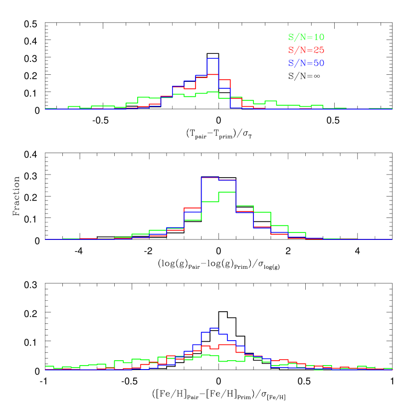
Figure 20: The effect of $S/N$ on the SSPP-determined atmospheric parameters. To isolate the difference degraded $S/N$ has on the SSPP measurements, we calculate the difference between the values determined for the pairs and the primaries at a given $S/N$ and divide it by the dispersion in that parameter determined by the SSPP for the primaries at that $S/N$ ($\sigma$). This compares the effect of binarity on a parameter at a given $S/N$ to the expected spread at that $S/N$. The top plot examines temperature, the middle surface gravity, and the bottom metallicity. The original infinite $S/N$ models are plotted in black, models with $S/N$ of 50 are in blue, $S/N$ of 25 are in red, and lastly $S/N$ of 10 is plotted in green.

Table 1: Number and Percentage of blends in the G-K dwarf range

Primary Distribution	Secondary Distribution	[Fe/H]	Primaries	Pairs	Percentage
Salpeter	Salpeter	-0.5	2566$\pm$ 7	1898$\pm$11	74$\pm$0.63
	Chabrier	-0.5	2530$\pm$12	1886$\pm$11	75$\pm$0.75
	Kroupa	-0.5	2526$\pm$ 9	1955$\pm$ 9	77$\pm$0.59
	DM	-0.5	2538$\pm$11	1930$\pm$ 8	76$\pm$0.60
	Halbwachs	-0.5	2554$\pm$18	2000$\pm$13	78$\pm$0.96
Kroupa	Salpeter	-0.5	2538$\pm$11	1873$\pm$ 9	74$\pm$0.66
	Chabrier	-0.5	2526$\pm$11	1893$\pm$ 8	75$\pm$0.62
	Kroupa	-0.5	2525$\pm$15	1974$\pm$17	78$\pm$1.07
	DM	-0.5	2526$\pm$11	1931$\pm$ 9	76$\pm$0.65
	Halbwachs	-0.5	2570$\pm$ 8	2016$\pm$12	78$\pm$0.68
Chabrier	Salpeter	-0.5	2670$\pm$11	1996$\pm$ 9	75$\pm$0.60
	Chabrier	-0.5	2678$\pm$12	2027$\pm$11	76$\pm$0.71
	Kroupa	-0.5	2662$\pm$12	2103$\pm$15	79$\pm$0.82
	DM	-0.5	2657$\pm$12	2065$\pm$10	78$\pm$0.67
	Halbwachs	-0.5	2660$\pm$13	2124$\pm$13	80$\pm$0.79
Salpeter	Salpeter	-1.0	2285$\pm$11	2262$\pm$12	99$\pm$0.73
	Chabrier	-1.0	2265$\pm$ 6	2288$\pm$11	101$\pm$0.56
	Kroupa	-1.0	2251$\pm$13	2321$\pm$14	103$\pm$0.83
	DM	-1.0	2289$\pm$17	2337$\pm$15	102$\pm$0.99
	Halbwachs	-1.0	2273$\pm$11	2331$\pm$12	103$\pm$0.72
Kroupa	Salpeter	-1.0	2259$\pm$ 5	2225$\pm$ 7	98$\pm$0.38
	Chabrier	-1.0	2256$\pm$12	2277$\pm$11	101$\pm$0.72
	Kroupa	-1.0	2255$\pm$ 9	2317$\pm$10	103$\pm$0.57
	DM	-1.0	2231$\pm$10	2302$\pm$ 6	103$\pm$0.50
	Halbwachs	-1.0	2263$\pm$10	2335$\pm$ 9	103$\pm$0.58
Chabrier	Salpeter	-1.0	2253$\pm$ 9	2237$\pm$ 9	99$\pm$0.60
	Chabrier	-1.0	2241$\pm$11	2270$\pm$14	101$\pm$0.79
	Kroupa	-1.0	2244$\pm$ 7	2342$\pm$13	104$\pm$0.63
	DM	-1.0	2252$\pm$12	2326$\pm$13	103$\pm$0.77
	Halbwachs	-1.0	2258$\pm$14	2337$\pm$11	103$\pm$0.78
Salpeter	Salpeter	-1.5	3310$\pm$13	2712$\pm$12	82$\pm$0.61
	Chabrier	-1.5	3325$\pm$11	2697$\pm$12	81$\pm$0.55
	Kroupa	-1.5	3301$\pm$10	2786$\pm$14	84$\pm$0.58
	DM	-1.5	3322$\pm$15	2786$\pm$16	84$\pm$0.74
	Halbwachs	-1.5	3316$\pm$14	2775$\pm$ 9	84$\pm$0.55
Kroupa	Salpeter	-1.5	3280$\pm$21	2695$\pm$16	82$\pm$0.88
	Chabrier	-1.5	3290$\pm$12	2673$\pm$10	81$\pm$0.53
	Kroupa	-1.5	3294$\pm$16	2788$\pm$13	85$\pm$0.67
	DM	-1.5	3262$\pm$19	2774$\pm$14	85$\pm$0.77
	Halbwachs	-1.5	3290$\pm$25	2742$\pm$20	83$\pm$1.05
Chabrier	Salpeter	-1.5	3173$\pm$17	2618$\pm$15	83$\pm$0.81
	Chabrier	-1.5	3166$\pm$16	2576$\pm$17	81$\pm$0.83
	Kroupa	-1.5	3168$\pm$12	2708$\pm$ 7	85$\pm$0.44
	DM	-1.5	3141$\pm$ 8	2685$\pm$12	85$\pm$0.53
	Halbwachs	-1.5	3145$\pm$14	2666$\pm$13	85$\pm$0.66
Salpeter	Salpeter	-2.0	3188$\pm$23	3007$\pm$21	94$\pm$1.01
	Chabrier	-2.0	3227$\pm$14	3073$\pm$14	95$\pm$0.63
	Kroupa	-2.0	3234$\pm$17	3186$\pm$18	99$\pm$0.77
	DM	-2.0	3230$\pm$18	3117$\pm$15	97$\pm$0.73
	Halbwachs	-2.0	3226$\pm$15	3082$\pm$12	96$\pm$0.60
Kroupa	Salpeter	-2.0	3159$\pm$13	2991$\pm$10	95$\pm$0.55
	Chabrier	-2.0	3168$\pm$ 7	3014$\pm$10	95$\pm$0.41
	Kroupa	-2.0	3191$\pm$15	3143$\pm$14	98$\pm$0.65
	DM	-2.0	3182$\pm$18	3066$\pm$12	96$\pm$0.67
	Halbwachs	-2.0	3182$\pm$17	3051$\pm$23	96$\pm$0.93
Chabrier	Salpeter	-2.0	3032$\pm$12	2876$\pm$12	95$\pm$0.58
	Chabrier	-2.0	3011$\pm$13	2875$\pm$13	95$\pm$0.63
	Kroupa	-2.0	3008$\pm$14	3003$\pm$ 9	100$\pm$0.56
	DM	-2.0	3015$\pm$13	2921$\pm$15	97$\pm$0.67
	Halbwachs	-2.0	3016$\pm$14	2895$\pm$12	96$\pm$0.63
Salpeter	Salpeter	-2.5	3866$\pm$14	3470$\pm$14	90$\pm$0.53
	Chabrier	-2.5	3860$\pm$16	3428$\pm$15	89$\pm$0.61
	Kroupa	-2.5	3851$\pm$17	3514$\pm$18	91$\pm$0.68
	DM	-2.5	3842$\pm$ 8	3457$\pm$13	90$\pm$0.42
	Halbwachs	-2.5	3845$\pm$20	3464$\pm$16	90$\pm$0.70
Kroupa	Salpeter	-2.5	3807$\pm$15	3409$\pm$10	90$\pm$0.48
	Chabrier	-2.5	3798$\pm$19	3364$\pm$17	89$\pm$0.71
	Kroupa	-2.5	3812$\pm$12	3487$\pm$ 9	91$\pm$0.39
	DM	-2.5	3781$\pm$12	3414$\pm$18	90$\pm$0.61
	Halbwachs	-2.5	3814$\pm$13	3447$\pm$10	90$\pm$0.45
Chabrier	Salpeter	-2.5	3556$\pm$19	3197$\pm$17	90$\pm$0.76
	Chabrier	-2.5	3560$\pm$16	3170$\pm$14	89$\pm$0.63
	Kroupa	-2.5	3567$\pm$14	3276$\pm$12	92$\pm$0.53
	DM	-2.5	3567$\pm$14	3251$\pm$14	91$\pm$0.57
	Halbwachs	-2.5	3569$\pm$17	3248$\pm$15	91$\pm$0.65

Note. — The numbers of primaries and pairs in the G-K color cut range for our models. A target must be within 0.48$\leq$$(g-r)_{O}$$\leq$0.75 to be selected as a G or K dwarf by SEGUE. In general, there are fewer photometrically blended pairs within the color cut than there are primaries, indicating that the addition of a secondary is more likely to bump a target out of G-K color range than in. Note, however, that for [Fe/H]=$-$1.0, there are more blended pairs in range than primaries. In general, 90$\pm$2% of the primaries within the G-K dwarf color cut remain there when blended with a secondary, indicating that there is a noticeable, but not large, difference between the statistics with binary contamination.

Table 2: Parameters for the synthetic spectra modeled

M (M⊙)	[Fe/H]	T (K)	$\log g$	$\log(L/L_{\odot})$	u	g	r	i	z
0.10	-0.5	3275	5.35	-2.89	18.40	14.80	13.20	12.15	11.60
0.15	-0.5	3325	5.20	-2.51	17.10	13.75	12.20	11.20	10.70
0.20	-0.5	3400	5.10	-2.26	16.20	13.00	11.40	10.50	10.10
0.25	-0.5	3500	5.00	-2.07	15.40	12.30	10.80	10.00	9.60
0.30	-0.5	3550	5.00	-1.92	14.90	11.80	10.35	9.60	9.20
0.35	-0.5	3625	4.90	-1.77	14.30	11.35	9.90	9.20	8.80
0.40	-0.5	3700	4.90	-1.62	13.80	10.90	9.45	8.80	8.50
0.45	-0.5	3800	4.80	-1.46	13.20	10.30	8.95	8.30	8.10
0.50	-0.5	3950	4.80	-1.29	12.60	9.70	8.40	7.90	7.70
0.55	-0.5	4150	4.70	-1.12	11.85	9.10	7.80	7.40	7.20
0.60	-0.5	4425	4.70	-0.94	11.00	8.30	7.30	6.90	6.80
0.65	-0.5	4750	4.70	-0.77	10.00	7.60	6.70	6.40	6.40
0.70	-0.5	5050	4.65	-0.60	9.00	6.90	6.20	6.00	6.00
0.75	-0.5	5350	4.60	-0.45	8.10	6.40	5.80	5.60	5.70
0.80	-0.5	5600	4.60	-0.31	7.40	5.90	5.40	5.30	5.30
0.85	-0.5	5850	4.60	-0.17	6.80	5.50	5.10	5.00	5.05
0.90	-0.5	6050	4.50	-0.03	6.25	5.10	4.80	4.70	4.75
0.95	-0.5	6250	4.45	0.10	5.80	4.70	4.40	4.40	4.50
1.00	-0.5	6450	4.40	0.24	5.40	4.40	4.10	4.10	4.20
0.10	-1.0	3325	5.40	-2.89	18.50	14.70	13.00	12.10	11.60
0.15	-1.0	3450	5.20	-2.46	16.80	13.40	11.80	10.95	10.60
0.20	-1.0	3575	5.10	-2.20	15.70	12.50	10.90	10.20	9.90
0.25	-1.0	3675	5.05	-2.00	14.90	11.80	10.30	9.70	9.40
0.30	-1.0	3750	5.00	-1.84	14.30	11.30	9.90	9.30	9.00
0.35	-1.0	3800	4.95	-1.70	13.80	10.90	9.50	8.90	8.70
0.40	-1.0	3900	4.90	-1.55	13.20	10.40	9.00	8.50	8.30
0.45	-1.0	4025	4.80	-1.38	12.50	9.80	8.50	8.10	7.90
0.50	-1.0	4200	4.80	-1.19	11.70	9.10	8.00	7.60	7.40
0.55	-1.0	4500	4.70	-1.00	10.80	8.30	7.40	7.05	7.00
0.60	-1.0	4850	4.70	-0.81	9.60	7.60	6.80	6.60	6.50
0.65	-1.0	5175	4.70	-0.64	8.60	6.90	6.30	6.10	6.10
0.70	-1.0	5500	4.70	-0.48	7.70	6.40	5.90	5.70	5.80
0.75	-1.0	5775	4.60	-0.32	7.05	5.90	5.50	5.40	5.40
0.80	-1.0	6050	4.60	-0.17	6.50	5.50	5.10	5.00	5.10
0.85	-1.0	6300	4.50	-0.03	6.00	5.10	4.80	4.70	4.80
0.90	-1.0	6525	4.50	0.12	5.60	4.70	4.45	4.40	4.50
0.95	-1.0	6725	4.40	0.26	5.20	4.30	4.10	4.10	4.20
1.00	-1.0	6975	4.40	0.40	4.90	3.90	3.80	3.80	3.90
0.10	-1.5	3400	5.40	-2.87	18.45	14.50	12.80	11.90	11.60
0.15	-1.5	3600	5.20	-2.40	16.20	12.90	11.40	10.70	10.40
0.20	-1.5	3750	5.10	-2.13	15.05	12.00	10.60	10.00	9.75
0.25	-1.5	3850	5.10	-1.94	14.30	11.40	10.00	9.50	9.30
0.30	-1.5	3900	5.00	-1.78	13.70	10.90	9.60	9.10	8.90
0.35	-1.5	3975	5.00	-1.64	13.10	10.50	9.20	8.70	8.50
0.40	-1.5	4050	4.90	-1.50	12.60	10.00	8.80	8.30	8.20
0.45	-1.5	4200	4.90	-1.33	11.85	9.40	8.30	7.90	7.75
0.50	-1.5	4425	4.80	-1.14	11.00	8.70	7.80	7.40	7.30
0.55	-1.5	4725	4.80	-0.94	9.90	8.00	7.20	6.90	6.80
0.60	-1.5	5075	4.75	-0.76	8.80	7.30	6.65	6.40	6.40
0.65	-1.5	5400	4.70	-0.58	7.90	6.70	6.20	6.00	6.00
0.70	-1.5	5725	4.70	-0.42	7.20	6.20	5.80	5.60	5.70
0.75	-1.5	6000	4.60	-0.26	6.70	5.70	5.40	5.30	5.35
0.80	-1.5	6300	4.60	-0.11	6.20	5.30	5.00	4.90	5.00
0.85	-1.5	6550	4.55	0.04	5.80	4.90	4.70	4.60	4.70
0.90	-1.5	6825	4.50	0.18	5.40	4.50	4.30	4.30	4.40
0.95	-1.5	7100	4.45	0.32	5.00	4.10	4.00	4.00	4.10
1.00	-1.5	7425	4.40	0.48	4.65	3.70	3.60	3.65	3.80
0.10	-2.0	3450	5.40	-2.86	18.20	14.30	12.60	11.80	11.50
0.15	-2.0	3750	5.20	-2.34	15.50	12.50	11.10	10.50	10.30
0.20	-2.0	3900	5.10	-2.07	14.30	11.60	10.30	9.80	9.60
0.25	-2.0	4000	5.10	-1.87	13.50	11.00	9.80	9.30	9.10
0.30	-2.0	4075	5.00	-1.71	12.90	10.50	9.30	8.90	8.70
0.35	-2.0	4150	5.00	-1.59	12.50	10.10	9.00	8.60	8.40
0.40	-2.0	4225	5.00	-1.47	12.00	9.70	8.70	8.20	8.10
0.45	-2.0	4350	4.90	-1.29	11.30	9.10	8.20	7.80	7.70
0.50	-2.0	4575	4.80	-1.11	10.40	8.50	7.60	7.30	7.20
0.55	-2.0	4850	4.80	-0.92	9.40	7.80	7.10	6.80	6.80
0.60	-2.0	5175	4.80	-0.74	8.50	7.20	6.60	6.40	6.40
0.65	-2.0	5500	4.70	-0.56	7.70	6.60	6.20	6.00	6.00
0.70	-2.0	5825	4.70	-0.39	7.10	6.10	5.70	5.60	5.70
0.75	-2.0	6125	4.65	-0.24	6.50	5.70	5.40	5.30	5.30
0.80	-2.0	6425	4.60	-0.08	6.05	5.20	5.00	4.90	5.00
0.85	-2.0	6700	4.60	0.06	5.70	4.80	4.60	4.60	4.70
0.90	-2.0	6975	4.50	0.21	5.30	4.40	4.30	4.30	4.40
0.95	-2.0	7300	4.50	0.35	4.90	4.00	3.90	4.00	4.10
1.00	-2.0	7725	4.40	0.51	4.60	3.60	3.60	3.60	3.80
0.10	-2.5	3500	5.40	-2.84	18.00	14.00	12.40	11.70	11.40
0.15	-2.5	3925	5.20	-2.29	14.80	12.10	10.80	10.30	10.10
0.20	-2.5	4075	5.15	-2.01	13.60	11.25	10.10	9.60	9.40
0.25	-2.5	4175	5.10	-1.81	12.90	10.60	9.55	9.10	8.90
0.30	-2.5	4250	5.00	-1.65	12.30	10.10	9.10	8.70	8.55
0.35	-2.5	4325	5.00	-1.52	11.80	9.80	8.80	8.40	8.20
0.40	-2.5	4400	5.00	-1.40	11.40	9.40	8.40	8.10	7.90
0.45	-2.5	4500	4.90	-1.25	10.80	8.90	8.00	7.70	7.60
0.50	-2.5	4675	4.90	-1.09	10.00	8.40	7.60	7.25	7.20
0.55	-2.5	4925	4.80	-0.91	9.15	7.80	7.10	6.80	6.80
0.60	-2.5	5225	4.80	-0.73	8.30	7.20	6.60	6.40	6.40
0.65	-2.5	5550	4.70	-0.55	7.60	6.60	6.15	6.00	6.00
0.70	-2.5	5850	4.70	-0.39	7.00	6.10	5.70	5.60	5.70
0.75	-2.5	6175	4.70	-0.23	6.50	5.65	5.35	5.30	5.30
0.80	-2.5	6475	4.60	-0.07	6.00	5.20	5.00	4.90	5.00
0.85	-2.5	6750	4.60	0.07	5.60	4.80	4.60	4.60	4.70
0.90	-2.5	7075	4.50	0.22	5.30	4.40	4.30	4.30	4.40
0.95	-2.5	7400	4.50	0.36	4.90	4.00	3.90	3.95	4.10
1.00	-2.5	7850	4.45	0.52	4.55	3.60	3.55	3.60	3.80

Note. — Parameters for the synthetic spectra modeled with MARCS model atmospheres in conjunction with TurboSpectrum. These values are determined from the Dartmouth isochrones (Dotter et al., 2008).

Table 3: Properties of the control group of primaries analyzed by the SSPP

MPrim	Model Teff	SSPP Teff	Model [Fe/H]	SSPP [Fe/H]	Model $\log g$	SSPP $\log g$	Model [$\alpha$/Fe]	SSPP [$\alpha$/Fe]	u	g	r	i	z	(g-r)
0.50	3950	4166$\pm$28	-0.5	-0.46$\pm$0.03	4.8	4.65$\pm$0.02	0.2	-	12.56	9.73	8.4	7.87	7.66	1.33
0.55	4150	4249$\pm$50	-0.5	-0.41$\pm$0.09	4.7	4.67$\pm$0.17	0.2	-	11.85	9.07	7.84	7.39	7.24	1.23
0.60	4425	4453$\pm$48	-0.5	-0.37$\pm$0.09	4.7	4.78$\pm$0.25	0.2	-	11.04	8.33	7.26	6.91	6.82	1.07
0.65	4750	4721$\pm$67	-0.5	-0.50$\pm$0.01	4.7	4.51$\pm$0.09	0.2	0.38$\pm$0.01	9.96	7.58	6.71	6.44	6.4	0.87
0.70	5050	4989$\pm$36	-0.5	-0.46$\pm$0.03	4.7	4.48$\pm$0.05	0.2	0.38$\pm$0.04	8.96	6.94	6.23	6.02	6.01	0.71
0.75	5350	5374$\pm$69	-0.5	-0.22$\pm$0.01	4.6	4.48$\pm$0.06	0.2	0.45$\pm$0.03	8.09	6.4	5.81	5.64	5.66	0.59
0.80	5600	5604$\pm$45	-0.5	-0.24$\pm$0.03	4.6	4.46$\pm$0.07	0.2	0.41$\pm$0.01	7.36	5.93	5.43	5.29	5.34	0.50
0.85	5850	5884$\pm$76	-0.5	-0.24$\pm$0.01	4.6	4.44$\pm$0.08	0.2	0.23$\pm$0.03	6.78	5.51	5.09	4.98	5.05	0.42
0.90	6050	6074$\pm$67	-0.5	-0.27$\pm$0.02	4.5	4.50$\pm$0.08	0.2	0.12$\pm$0.03	6.25	5.12	4.76	4.67	4.75	0.36
0.95	6250	6279$\pm$51	-0.5	-0.34$\pm$0.04	4.5	4.40$\pm$0.05	0.2	0.17$\pm$0.08	5.79	4.74	4.43	4.36	4.46	0.31
1.00	6450	6536$\pm$32	-0.5	-0.35$\pm$0.06	4.4	4.02$\pm$0.08	0.2	0.10$\pm$0.02	5.37	4.36	4.11	4.06	4.17	0.25
0.50	4200	4304$\pm$46	-1.0	-0.94$\pm$0.07	4.8	4.57$\pm$0.09	0.4	-	11.69	9.12	7.98	7.56	7.42	1.14
0.55	4500	4452$\pm$14	-1.0	-0.98$\pm$0.01	4.7	4.77$\pm$0.17	0.4	-	10.76	8.34	7.38	7.05	6.96	0.96
0.60	4850	4778$\pm$59	-1.0	-1.02$\pm$0.04	4.7	4.41$\pm$0.09	0.4	0.53$\pm$0.01	9.61	7.57	6.81	6.56	6.52	0.76
0.65	5175	5182$\pm$26	-1.0	-0.89$\pm$0.04	4.7	4.51$\pm$0.06	0.4	0.49$\pm$0.01	8.58	6.93	6.32	6.12	6.12	0.61
0.70	5500	5548$\pm$53	-1.0	-0.69$\pm$0.02	4.7	4.40$\pm$0.10	0.4	0.38$\pm$0.04	7.72	6.39	5.89	5.73	5.76	0.50
0.75	5775	5780$\pm$57	-1.0	-0.83$\pm$0.06	4.6	4.47$\pm$0.06	0.4	0.42$\pm$0.02	7.05	5.92	5.5	5.37	5.43	0.42
0.80	6050	6080$\pm$61	-1.0	-0.86$\pm$0.06	4.6	4.53$\pm$0.06	0.4	0.31$\pm$0.01	6.5	5.48	5.14	5.04	5.12	0.34
0.85	6300	6298$\pm$46	-1.0	-0.89$\pm$0.04	4.5	4.56$\pm$0.05	0.4	0.26$\pm$0.03	6.03	5.07	4.79	4.72	4.82	0.28
0.90	6525	6575$\pm$45	-1.0	-0.94$\pm$0.02	4.5	4.54$\pm$0.09	0.4	0.32$\pm$0.05	5.61	4.68	4.45	4.4	4.51	0.23
0.95	6725	6829$\pm$29	-1.0	-0.82$\pm$0.01	4.4	4.12$\pm$0.19	0.4	0.12$\pm$0.02	5.23	4.3	4.11	4.08	4.21	0.19
1.00	6975	7073$\pm$65	-1.0	-0.93$\pm$0.03	4.4	3.88$\pm$0.24	0.4	0.24$\pm$0.03	4.87	3.92	3.77	3.77	3.92	0.15
0.50	4425	4431$\pm$35	-1.5	-1.37$\pm$0.05	4.8	4.60$\pm$0.06	0.4	-	10.98	8.72	7.76	7.4	7.29	0.96
0.55	4725	4677$\pm$74	-1.5	-1.50$\pm$0.04	4.8	4.33$\pm$0.13	0.4	0.52$\pm$0.02	9.91	7.96	7.18	6.89	6.83	0.78
0.60	5075	5085$\pm$39	-1.5	-1.32$\pm$0.00	4.7	4.35$\pm$0.17	0.4	0.55$\pm$0.04	8.83	7.28	6.65	6.42	6.41	0.63
0.65	5400	5453$\pm$63	-1.5	-1.30$\pm$0.03	4.7	4.21$\pm$0.22	0.4	0.60$\pm$0.08	7.94	6.7	6.18	6	6.02	0.52
0.70	5725	5743$\pm$64	-1.5	-1.35$\pm$0.03	4.7	4.34$\pm$0.15	0.4	0.39$\pm$0.02	7.24	6.19	5.77	5.63	5.68	0.42
0.75	6000	6024$\pm$61	-1.5	-1.42$\pm$0.05	4.6	4.57$\pm$0.05	0.4	0.40$\pm$0.03	6.66	5.73	5.39	5.28	5.35	0.34
0.80	6300	6286$\pm$48	-1.5	-1.54$\pm$0.02	4.6	4.31$\pm$0.13	0.4	0.32$\pm$0.07	6.17	5.3	5.02	4.94	5.04	0.28
0.85	6550	6582$\pm$38	-1.5	-1.49$\pm$0.02	4.5	4.12$\pm$0.21	0.4	0.36$\pm$0.04	5.76	4.9	4.68	4.63	4.74	0.22
0.90	6825	6868$\pm$33	-1.5	-1.55$\pm$0.06	4.5	4.11$\pm$0.26	0.4	0.24$\pm$0.03	5.37	4.5	4.32	4.3	4.43	0.18
0.95	7100	7137$\pm$45	-1.5	-1.49$\pm$0.01	4.5	4.11$\pm$0.21	0.4	0.19$\pm$0.01	5.01	4.11	3.98	3.99	4.14	0.13
1.00	7425	7471$\pm$103	-1.5	-1.51$\pm$0.02	4.4	4.20$\pm$0.21	0.4	-	4.65	3.69	3.62	3.65	3.83	0.07
0.50	4575	4601$\pm$84	-2.0	-1.82$\pm$0.06	4.8	3.80$\pm$0.37	0.4	0.48$\pm$0.01	10.4	8.49	7.64	7.31	7.22	0.85
0.55	4850	4832$\pm$49	-2.0	-1.90$\pm$0.09	4.8	3.92$\pm$0.33	0.4	0.50$\pm$0.02	9.41	7.82	7.11	6.83	6.78	0.71
0.60	5175	5231$\pm$59	-2.0	-1.80$\pm$0.06	4.8	4.54$\pm$0.03	0.4	0.41$\pm$0.01	8.47	7.19	6.6	6.38	6.37	0.59
0.65	5500	5566$\pm$69	-2.0	-1.73$\pm$0.01	4.7	3.96$\pm$0.36	0.4	0.32$\pm$0.06	7.69	6.63	6.16	5.98	6	0.47
0.70	5825	5838$\pm$65	-2.0	-1.96$\pm$0.06	4.7	4.36$\pm$0.12	0.4	0.32$\pm$0.04	7.06	6.13	5.74	5.61	5.66	0.39
0.75	6125	6130$\pm$56	-2.0	-2.08$\pm$0.15	4.7	4.14$\pm$0.02	0.4	0.31$\pm$0.01	6.52	5.67	5.36	5.26	5.33	0.31
0.80	6425	6428$\pm$53	-2.0	-2.05$\pm$0.01	4.6	4.31$\pm$0.13	0.4	0.11$\pm$0.02	6.05	5.24	4.99	4.92	5.02	0.25
0.85	6700	6732$\pm$31	-2.0	-2.06$\pm$0.04	4.6	4.17$\pm$0.22	0.4	0.11$\pm$0.00	5.66	4.84	4.64	4.6	4.72	0.20
0.90	6975	7047$\pm$40	-2.0	-2.08$\pm$0.04	4.5	4.14$\pm$0.25	0.4	0.21$\pm$0.05	5.29	4.44	4.29	4.28	4.42	0.15
0.95	7300	7364$\pm$106	-2.0	-2.10$\pm$0.05	4.5	4.09$\pm$0.21	0.4	0.33$\pm$0.05	4.94	4.03	3.94	3.96	4.13	0.09
1.00	7725	7745$\pm$125	-2.0	-2.13$\pm$0.05	4.4	4.19$\pm$0.03	0.4	-	4.58	3.59	3.56	3.63	3.83	0.03
0.50	4675	4650$\pm$78	-2.5	-2.36$\pm$0.00	4.9	3.74$\pm$0.43	0.4	0.48$\pm$0.05	10.01	8.37	7.58	7.25	7.17	0.79
0.55	4925	4979$\pm$75	-2.5	-2.37$\pm$0.03	4.8	4.61$\pm$0.01	0.4	0.41$\pm$0.01	9.15	7.76	7.08	6.81	6.76	0.68
0.60	5225	5284$\pm$60	-2.5	-2.31$\pm$0.03	4.8	4.63$\pm$0.04	0.4	0.21$\pm$0.02	8.31	7.16	6.6	6.38	6.37	0.56
0.65	5550	5586$\pm$66	-2.5	-2.37$\pm$0.25	4.7	3.64$\pm$0.43	0.4	0.27$\pm$0.07	7.59	6.61	6.15	5.98	6	0.46
0.70	5850	5851$\pm$62	-2.5	-2.60$\pm$0.25	4.7	4.10$\pm$0.18	0.4	0.33$\pm$0.02	6.98	6.11	5.74	5.61	5.66	0.37
0.75	6175	6167$\pm$53	-2.5	-2.62$\pm$0.02	4.7	4.08$\pm$0.18	0.4	0.29$\pm$0.04	6.46	5.65	5.35	5.26	5.33	0.30
0.80	6475	6490$\pm$39	-2.5	-2.61$\pm$0.04	4.6	4.05$\pm$0.22	0.4	0.16$\pm$0.05	6.01	5.22	4.99	4.92	5.02	0.23
0.85	6750	6788$\pm$27	-2.5	-2.68$\pm$0.04	4.6	4.02$\pm$0.26	0.4	0.31$\pm$0.07	5.63	4.82	4.63	4.6	4.72	0.19
0.90	7075	7198$\pm$57	-2.5	-2.60$\pm$0.05	4.5	4.57$\pm$0.21	0.4	0.23$\pm$0.04	5.26	4.42	4.29	4.28	4.43	0.13
0.95	7400	7537$\pm$96	-2.5	-2.50$\pm$0.03	4.5	4.43$\pm$0.11	0.4	-	4.91	4	3.93	3.95	4.13	0.07
1.00	7850	8179$\pm$84	-2.5	-2.34$\pm$0.04	4.5	4.61$\pm$0.03	0.4	-	4.55	3.56	3.55	3.62	3.83	0.01

Note. — The SSPP parameter determinations for the control group as compared to the actual synthetic model values. Note that there are no temperature or metallicity measurements for stars less than 4000 K, as the SSPP does not work for these temperatures. The parameters for spectral modeling are listed as well.

Table 4: Properties of the blended binaries analyzed by the SSPP

MPrim	MSec	[Fe/H]model	Teff	[Fe/H]	$\log g$	[$\alpha$/Fe]	u	g	r	i	z	(g-r)
0.50	0.10	-0.5	-	-	-	-	12.56	9.72	8.39	7.85	7.63	1.33
0.50	0.15	-0.5	-	-	-	-	12.55	9.70	8.37	7.82	7.60	1.33
0.50	0.20	-0.5	-	-	-	-	12.52	9.68	8.34	7.78	7.55	1.34
0.50	0.25	-0.5	-	-	-	-	12.49	9.64	8.29	7.72	7.49	1.35
0.50	0.30	-0.5	-	-	-	-	12.44	9.58	8.24	7.66	7.42	1.34
0.50	0.35	-0.5	-	-	-	-	12.37	9.51	8.16	7.58	7.34	1.35
0.50	0.40	-0.5	-	-	-	-	12.26	9.41	8.05	7.47	7.24	1.36
0.50	0.45	-0.5	-	-	-	-	12.09	9.24	7.89	7.32	7.10	1.35
0.50	0.50	-0.5	4166$\pm$27	-0.41$\pm$0.04	4.56$\pm$0.08	-	11.81	8.98	7.65	7.11	6.91	1.33
0.55	0.10	-0.5	4238$\pm$53	-0.43$\pm$0.11	4.56$\pm$0.08	-	11.85	9.06	7.83	7.38	7.22	1.23
0.55	0.15	-0.5	4232$\pm$53	-0.44$\pm$0.12	4.56$\pm$0.12	-	11.84	9.05	7.82	7.36	7.19	1.23
0.55	0.20	-0.5	4224$\pm$53	-0.43$\pm$0.13	4.56$\pm$0.13	-	11.83	9.04	7.80	7.33	7.16	1.24
0.55	0.25	-0.5	4224$\pm$50	-0.43$\pm$0.14	4.55$\pm$0.12	-	11.81	9.02	7.77	7.29	7.12	1.25
0.55	0.30	-0.5	4212$\pm$51	-0.46$\pm$0.13	4.60$\pm$0.15	-	11.79	8.99	7.74	7.25	7.07	1.25
0.55	0.35	-0.5	4189$\pm$57	-0.42$\pm$0.19	4.56$\pm$0.13	-	11.75	8.94	7.69	7.19	7.01	1.25
0.55	0.40	-0.5	4185$\pm$57	-0.43$\pm$0.20	4.56$\pm$0.13	-	11.69	8.88	7.62	7.12	6.93	1.26
0.55	0.45	-0.5	4180$\pm$57	-0.44$\pm$0.07	4.59$\pm$0.14	-	11.58	8.77	7.51	7.01	6.83	1.26
0.55	0.50	-0.5	4201$\pm$53	-0.48$\pm$0.15	4.66$\pm$0.18	-	11.40	8.60	7.33	6.85	6.68	1.27
0.55	0.55	-0.5	4243$\pm$54	-0.42$\pm$0.13	4.55$\pm$0.12	-	11.10	8.32	7.09	6.64	6.49	1.23
0.60	0.10	-0.5	4410$\pm$19	-0.24$\pm$0.08	4.83$\pm$0.25	-	11.04	8.33	7.26	6.90	6.80	1.07
0.60	0.15	-0.5	4416$\pm$15	-0.20$\pm$0.12	4.60$\pm$0.12	-	11.04	8.32	7.25	6.89	6.79	1.07
0.60	0.20	-0.5	4403$\pm$12	-0.33$\pm$0.01	4.67$\pm$0.17	-	11.03	8.31	7.24	6.87	6.76	1.07
0.60	0.25	-0.5	4382$\pm$6	-0.32$\pm$0.01	4.50$\pm$0.08	-	11.03	8.30	7.22	6.85	6.74	1.08
0.60	0.30	-0.5	4402$\pm$35	-0.26$\pm$0.09	4.66$\pm$0.18	-	11.01	8.29	7.20	6.82	6.70	1.09
0.60	0.35	-0.5	4391$\pm$33	-0.36$\pm$0.00	4.63$\pm$0.15	-	10.99	8.26	7.17	6.78	6.66	1.09
0.60	0.40	-0.5	4359$\pm$39	-0.32$\pm$0.05	4.59$\pm$0.14	-	10.96	8.23	7.12	6.73	6.60	1.11
0.60	0.45	-0.5	4384$\pm$37	-0.33$\pm$0.07	4.57$\pm$0.12	-	10.91	8.17	7.05	6.65	6.52	1.12
0.60	0.50	-0.5	4357$\pm$46	-0.28$\pm$0.13	4.55$\pm$0.11	-	10.80	8.06	6.94	6.53	6.41	1.12
0.60	0.55	-0.5	4361$\pm$35	-0.34$\pm$0.05	4.55$\pm$0.10	-	10.62	7.88	6.76	6.37	6.25	1.12
0.60	0.60	-0.5	4415$\pm$21	-0.32$\pm$0.01	4.85$\pm$0.25	-	10.29	7.58	6.51	6.15	6.06	1.07
0.65	0.10	-0.5	4642$\pm$51	-0.52$\pm$0.08	4.43$\pm$0.10	0.35$\pm$0.05	9.96	7.57	6.71	6.43	6.39	0.86
0.65	0.15	-0.5	4664$\pm$53	-0.54$\pm$0.08	4.51$\pm$0.10	0.37$\pm$0.05	9.96	7.57	6.70	6.43	6.38	0.87
0.65	0.20	-0.5	4662$\pm$50	-0.54$\pm$0.07	4.52$\pm$0.11	0.33$\pm$0.02	9.96	7.57	6.70	6.41	6.36	0.87
0.65	0.25	-0.5	4646$\pm$48	-0.57$\pm$0.08	4.47$\pm$0.09	0.32$\pm$0.00	9.95	7.56	6.69	6.40	6.34	0.87
0.65	0.30	-0.5	4630$\pm$43	-0.59$\pm$0.07	4.41$\pm$0.08	0.35$\pm$0.04	9.95	7.55	6.67	6.38	6.32	0.88
0.65	0.35	-0.5	4618$\pm$35	-0.55$\pm$0.09	4.42$\pm$0.09	0.22$\pm$0.05	9.94	7.54	6.65	6.35	6.28	0.89
0.65	0.40	-0.5	4606$\pm$40	-0.60$\pm$0.07	4.41$\pm$0.11	0.37$\pm$0.04	9.93	7.52	6.63	6.32	6.25	0.89
0.65	0.45	-0.5	4577$\pm$85	-0.48$\pm$0.14	4.67$\pm$0.15	0.34$\pm$0.02	9.91	7.49	6.58	6.26	6.19	0.91
0.65	0.50	-0.5	4557$\pm$86	-0.54$\pm$0.08	4.52$\pm$0.15	0.35$\pm$0.01	9.87	7.44	6.50	6.18	6.10	0.94
0.65	0.55	-0.5	4565$\pm$112	-0.53$\pm$0.06	4.66$\pm$0.16	0.32$\pm$0.01	9.79	7.33	6.38	6.06	5.99	0.95
0.65	0.60	-0.5	4548$\pm$84	-0.58$\pm$0.07	4.58$\pm$0.14	0.25$\pm$0.04	9.62	7.14	6.20	5.90	5.83	0.94
0.65	0.65	-0.5	4633$\pm$61	-0.58$\pm$0.06	4.49$\pm$0.13	0.28$\pm$0.02	9.21	6.82	5.96	5.69	5.64	0.86
0.70	0.10	-0.5	4963$\pm$37	-0.45$\pm$0.05	4.49$\pm$0.07	0.38$\pm$0.01	8.96	6.94	6.23	6.01	6.00	0.71
0.70	0.15	-0.5	4971$\pm$40	-0.45$\pm$0.05	4.49$\pm$0.06	0.36$\pm$0.00	8.96	6.93	6.23	6.01	6.00	0.70
0.70	0.20	-0.5	4941$\pm$40	-0.45$\pm$0.06	4.45$\pm$0.08	0.37$\pm$0.05	8.96	6.93	6.22	6.00	5.98	0.71
0.70	0.25	-0.5	4926$\pm$41	-0.56$\pm$0.05	4.42$\pm$0.08	0.40$\pm$0.01	8.96	6.93	6.21	5.99	5.97	0.72
0.70	0.30	-0.5	4909$\pm$43	-0.61$\pm$0.07	4.41$\pm$0.08	0.22$\pm$0.06	8.95	6.92	6.21	5.98	5.95	0.71
0.70	0.35	-0.5	4871$\pm$55	-0.54$\pm$0.05	4.27$\pm$0.14	0.21$\pm$0.10	8.95	6.92	6.19	5.96	5.93	0.73
0.70	0.40	-0.5	4818$\pm$39	-0.58$\pm$0.04	4.26$\pm$0.15	0.34$\pm$0.02	8.95	6.91	6.18	5.93	5.90	0.73
0.70	0.45	-0.5	4824$\pm$50	-0.55$\pm$0.04	4.26$\pm$0.13	0.39$\pm$0.03	8.94	6.89	6.14	5.89	5.86	0.75
0.70	0.50	-0.5	4776$\pm$47	-0.63$\pm$0.04	4.18$\pm$0.10	0.35$\pm$0.01	8.92	6.86	6.09	5.83	5.80	0.77
0.70	0.55	-0.5	4735$\pm$66	-0.63$\pm$0.06	4.25$\pm$0.15	0.27$\pm$0.03	8.89	6.79	6.01	5.75	5.71	0.78
0.70	0.60	-0.5	4716$\pm$71	-0.62$\pm$0.04	4.40$\pm$0.12	0.30$\pm$0.04	8.81	6.67	5.88	5.62	5.59	0.79
0.70	0.65	-0.5	4804$\pm$60	-0.56$\pm$0.06	4.35$\pm$0.12	0.26$\pm$0.06	8.60	6.46	5.69	5.45	5.43	0.77
0.70	0.70	-0.5	4977$\pm$37	-0.42$\pm$0.06	4.50$\pm$0.06	0.43$\pm$0.05	8.21	6.18	5.48	5.26	5.26	0.70
0.75	0.10	-0.5	5311$\pm$46	-0.35$\pm$0.06	4.46$\pm$0.06	0.36$\pm$0.01	8.09	6.40	5.81	5.63	5.66	0.59
0.75	0.15	-0.5	5309$\pm$46	-0.35$\pm$0.06	4.46$\pm$0.06	0.41$\pm$0.02	8.09	6.40	5.81	5.63	5.65	0.59
0.75	0.20	-0.5	5307$\pm$54	-0.31$\pm$0.05	4.41$\pm$0.07	0.36$\pm$0.01	8.09	6.40	5.80	5.62	5.64	0.60
0.75	0.25	-0.5	5307$\pm$51	-0.35$\pm$0.06	4.47$\pm$0.07	0.36$\pm$0.01	8.09	6.39	5.80	5.62	5.63	0.59
0.75	0.30	-0.5	5285$\pm$56	-0.37$\pm$0.06	4.42$\pm$0.07	0.36$\pm$0.01	8.09	6.39	5.79	5.61	5.62	0.60
0.75	0.35	-0.5	5276$\pm$62	-0.38$\pm$0.04	4.33$\pm$0.11	0.35$\pm$0.06	8.09	6.39	5.78	5.59	5.60	0.61
0.75	0.40	-0.5	5254$\pm$57	-0.40$\pm$0.05	4.34$\pm$0.11	0.36$\pm$0.03	8.09	6.38	5.77	5.58	5.58	0.61
0.75	0.45	-0.5	5201$\pm$53	-0.41$\pm$0.05	4.32$\pm$0.12	0.35$\pm$0.05	8.09	6.37	5.75	5.55	5.55	0.62
0.75	0.50	-0.5	5157$\pm$59	-0.44$\pm$0.03	4.28$\pm$0.12	0.37$\pm$0.04	8.08	6.35	5.71	5.50	5.50	0.64
0.75	0.55	-0.5	5091$\pm$60	-0.47$\pm$0.05	4.26$\pm$0.12	0.38$\pm$0.01	8.06	6.31	5.65	5.44	5.43	0.66
0.75	0.60	-0.5	4985$\pm$64	-0.58$\pm$0.07	4.39$\pm$0.10	0.35$\pm$0.02	8.03	6.23	5.56	5.34	5.34	0.67
0.75	0.65	-0.5	5096$\pm$51	-0.47$\pm$0.05	4.43$\pm$0.10	0.38$\pm$0.01	7.92	6.08	5.42	5.21	5.21	0.66
0.75	0.70	-0.5	5185$\pm$46	-0.34$\pm$0.05	4.48$\pm$0.06	0.36$\pm$0.02	7.69	5.88	5.25	5.06	5.07	0.63
0.75	0.75	-0.5	5323$\pm$56	-0.32$\pm$0.05	4.46$\pm$0.07	0.39$\pm$0.01	7.34	5.65	5.06	4.88	4.91	0.59
0.80	0.10	-0.5	5592$\pm$51	-0.37$\pm$0.05	4.44$\pm$0.06	0.32$\pm$0.01	7.36	5.93	5.43	5.29	5.34	0.50
0.80	0.15	-0.5	5585$\pm$49	-0.28$\pm$0.02	4.44$\pm$0.06	0.26$\pm$0.09	7.36	5.93	5.43	5.29	5.33	0.50
0.80	0.20	-0.5	5610$\pm$51	-0.33$\pm$0.05	4.47$\pm$0.06	0.36$\pm$0.02	7.36	5.92	5.43	5.28	5.33	0.49
0.80	0.25	-0.5	5577$\pm$48	-0.27$\pm$0.03	4.46$\pm$0.06	0.31$\pm$0.05	7.36	5.92	5.42	5.28	5.32	0.50
0.80	0.30	-0.5	5569$\pm$51	-0.31$\pm$0.04	4.46$\pm$0.06	0.35$\pm$0.02	7.36	5.92	5.42	5.27	5.31	0.50
0.80	0.35	-0.5	5552$\pm$49	-0.27$\pm$0.03	4.40$\pm$0.05	0.27$\pm$0.02	7.36	5.92	5.41	5.26	5.30	0.51
0.80	0.40	-0.5	5548$\pm$51	-0.34$\pm$0.07	4.43$\pm$0.05	0.16$\pm$0.07	7.36	5.92	5.41	5.25	5.28	0.51
0.80	0.45	-0.5	5533$\pm$51	-0.45$\pm$0.06	4.46$\pm$0.07	0.33$\pm$0.02	7.36	5.91	5.39	5.23	5.26	0.52
0.80	0.50	-0.5	5494$\pm$45	-0.42$\pm$0.06	4.47$\pm$0.08	0.34$\pm$0.01	7.35	5.89	5.36	5.19	5.22	0.53
0.80	0.55	-0.5	5438$\pm$52	-0.30$\pm$0.00	4.44$\pm$0.08	0.29$\pm$0.03	7.35	5.87	5.32	5.14	5.17	0.55
0.80	0.60	-0.5	5384$\pm$65	-0.44$\pm$0.06	4.52$\pm$0.07	0.33$\pm$0.02	7.33	5.81	5.25	5.07	5.09	0.56
0.80	0.65	-0.5	5400$\pm$52	-0.36$\pm$0.05	4.53$\pm$0.06	0.31$\pm$0.03	7.27	5.71	5.14	4.97	4.99	0.57
0.80	0.70	-0.5	5396$\pm$42	-0.35$\pm$0.04	4.54$\pm$0.07	0.36$\pm$0.04	7.14	5.57	5.01	4.84	4.87	0.56
0.80	0.75	-0.5	5504$\pm$44	-0.28$\pm$0.04	4.48$\pm$0.05	0.34$\pm$0.02	6.92	5.38	4.85	4.70	4.74	0.53
0.80	0.80	-0.5	5615$\pm$49	-0.42$\pm$0.03	4.47$\pm$0.06	0.32$\pm$0.01	6.61	5.17	4.68	4.54	4.59	0.49
0.85	0.10	-0.5	5829$\pm$46	-0.26$\pm$0.01	4.44$\pm$0.08	0.21$\pm$0.04	6.78	5.51	5.09	4.98	5.05	0.42
0.85	0.15	-0.5	5833$\pm$49	-0.27$\pm$0.00	4.38$\pm$0.05	0.17$\pm$0.01	6.78	5.51	5.09	4.97	5.04	0.42
0.85	0.20	-0.5	5825$\pm$47	-0.26$\pm$0.01	4.42$\pm$0.08	0.16$\pm$0.02	6.78	5.51	5.09	4.97	5.04	0.42
0.85	0.25	-0.5	5819$\pm$46	-0.26$\pm$0.01	4.41$\pm$0.08	0.17$\pm$0.02	6.78	5.51	5.09	4.97	5.03	0.42
0.85	0.30	-0.5	5812$\pm$50	-0.31$\pm$0.02	4.40$\pm$0.08	0.36$\pm$0.03	6.78	5.51	5.08	4.96	5.03	0.43
0.85	0.35	-0.5	5810$\pm$52	-0.36$\pm$0.04	4.42$\pm$0.09	0.41$\pm$0.02	6.78	5.51	5.08	4.96	5.02	0.43
0.85	0.40	-0.5	5796$\pm$49	-0.33$\pm$0.02	4.44$\pm$0.06	0.16$\pm$0.03	6.77	5.51	5.07	4.95	5.00	0.44
0.85	0.45	-0.5	5769$\pm$47	-0.37$\pm$0.06	4.39$\pm$0.07	0.22$\pm$0.03	6.77	5.50	5.06	4.93	4.98	0.44
0.85	0.50	-0.5	5762$\pm$44	-0.34$\pm$0.03	4.44$\pm$0.07	0.14$\pm$0.03	6.77	5.49	5.04	4.90	4.95	0.45
0.85	0.55	-0.5	5722$\pm$52	-0.42$\pm$0.07	4.48$\pm$0.05	0.32$\pm$0.02	6.77	5.47	5.01	4.87	4.91	0.46
0.85	0.60	-0.5	5675$\pm$49	-0.42$\pm$0.06	4.56$\pm$0.07	0.34$\pm$0.02	6.76	5.44	4.95	4.81	4.85	0.49
0.85	0.65	-0.5	5666$\pm$51	-0.43$\pm$0.05	4.56$\pm$0.05	0.31$\pm$0.01	6.72	5.36	4.87	4.73	4.77	0.49
0.85	0.70	-0.5	5657$\pm$44	-0.39$\pm$0.04	4.58$\pm$0.07	0.35$\pm$0.03	6.64	5.26	4.77	4.63	4.67	0.49
0.85	0.75	-0.5	5669$\pm$46	-0.35$\pm$0.03	4.49$\pm$0.07	0.38$\pm$0.04	6.49	5.12	4.64	4.51	4.56	0.48
0.85	0.80	-0.5	5755$\pm$50	-0.28$\pm$0.03	4.49$\pm$0.07	0.29$\pm$0.05	6.28	4.95	4.50	4.37	4.43	0.45
0.85	0.85	-0.5	5837$\pm$50	-0.27$\pm$0.00	4.45$\pm$0.05	0.29$\pm$0.02	6.02	4.76	4.34	4.23	4.30	0.42
0.90	0.10	-0.5	6048$\pm$47	-0.23$\pm$0.00	4.36$\pm$0.08	0.20$\pm$0.01	6.25	5.12	4.76	4.67	4.75	0.36
0.90	0.15	-0.5	6074$\pm$69	-0.24$\pm$0.02	4.36$\pm$0.09	0.30$\pm$0.02	6.25	5.12	4.76	4.66	4.75	0.36
0.90	0.20	-0.5	6042$\pm$46	-0.24$\pm$0.02	4.40$\pm$0.07	0.34$\pm$0.02	6.25	5.12	4.76	4.66	4.74	0.36
0.90	0.25	-0.5	6027$\pm$44	-0.28$\pm$0.04	4.41$\pm$0.07	0.18$\pm$0.02	6.25	5.12	4.76	4.66	4.74	0.36
0.90	0.30	-0.5	6072$\pm$66	-0.29$\pm$0.03	4.50$\pm$0.08	0.09$\pm$0.04	6.25	5.12	4.75	4.65	4.73	0.37
0.90	0.35	-0.5	6069$\pm$66	-0.28$\pm$0.00	4.50$\pm$0.07	0.24$\pm$0.08	6.25	5.12	4.75	4.65	4.73	0.37
0.90	0.40	-0.5	6019$\pm$47	-0.34$\pm$0.06	4.48$\pm$0.07	0.32$\pm$0.01	6.25	5.11	4.74	4.64	4.72	0.37
0.90	0.45	-0.5	6004$\pm$45	-0.33$\pm$0.06	4.50$\pm$0.06	0.16$\pm$0.02	6.25	5.11	4.74	4.63	4.70	0.37
0.90	0.50	-0.5	5991$\pm$46	-0.27$\pm$0.01	4.49$\pm$0.06	0.32$\pm$0.02	6.25	5.10	4.72	4.61	4.68	0.38
0.90	0.55	-0.5	5954$\pm$42	-0.44$\pm$0.08	4.50$\pm$0.06	0.20$\pm$0.06	6.24	5.09	4.70	4.58	4.65	0.39
0.90	0.60	-0.5	5915$\pm$46	-0.28$\pm$0.01	4.52$\pm$0.06	0.32$\pm$0.05	6.24	5.06	4.66	4.54	4.60	0.40
0.90	0.65	-0.5	5933$\pm$72	-0.39$\pm$0.06	4.50$\pm$0.06	0.31$\pm$0.04	6.21	5.01	4.59	4.47	4.54	0.42
0.90	0.70	-0.5	5863$\pm$39	-0.44$\pm$0.06	4.51$\pm$0.06	0.16$\pm$0.04	6.16	4.93	4.51	4.39	4.46	0.42
0.90	0.75	-0.5	5865$\pm$59	-0.42$\pm$0.06	4.57$\pm$0.07	0.09$\pm$0.02	6.07	4.83	4.41	4.29	4.36	0.42
0.90	0.80	-0.5	5931$\pm$73	-0.27$\pm$0.03	4.44$\pm$0.08	0.31$\pm$0.01	5.92	4.70	4.29	4.18	4.25	0.41
0.90	0.85	-0.5	5960$\pm$48	-0.29$\pm$0.01	4.48$\pm$0.08	0.32$\pm$0.03	5.73	4.55	4.16	4.06	4.14	0.39
0.90	0.90	-0.5	6073$\pm$68	-0.24$\pm$0.03	4.42$\pm$0.08	0.19$\pm$0.04	5.50	4.37	4.01	3.91	4.00	0.36
0.95	0.10	-0.5	6265$\pm$45	-0.31$\pm$0.04	4.53$\pm$0.06	0.29$\pm$0.03	5.79	4.74	4.43	4.36	4.46	0.31
0.95	0.15	-0.5	6263$\pm$45	-0.31$\pm$0.04	4.53$\pm$0.06	0.30$\pm$0.01	5.79	4.74	4.43	4.36	4.45	0.31
0.95	0.20	-0.5	6260$\pm$44	-0.29$\pm$0.03	4.54$\pm$0.06	0.28$\pm$0.03	5.79	4.74	4.43	4.36	4.45	0.31
0.95	0.25	-0.5	6259$\pm$44	-0.31$\pm$0.03	4.53$\pm$0.06	0.27$\pm$0.02	5.79	4.74	4.43	4.35	4.45	0.31
0.95	0.30	-0.5	6257$\pm$42	-0.22$\pm$0.00	4.50$\pm$0.06	0.16$\pm$0.04	5.79	4.73	4.43	4.35	4.44	0.30
0.95	0.35	-0.5	6252$\pm$44	-0.34$\pm$0.03	4.54$\pm$0.06	0.17$\pm$0.04	5.79	4.73	4.42	4.35	4.44	0.31
0.95	0.40	-0.5	6247$\pm$44	-0.30$\pm$0.04	4.53$\pm$0.05	0.28$\pm$0.01	5.79	4.73	4.42	4.34	4.43	0.31
0.95	0.45	-0.5	6227$\pm$42	-0.30$\pm$0.00	4.52$\pm$0.05	0.29$\pm$0.05	5.78	4.73	4.41	4.33	4.42	0.32
0.95	0.50	-0.5	6200$\pm$39	-0.34$\pm$0.00	4.64$\pm$0.00	0.16$\pm$0.04	5.78	4.73	4.40	4.32	4.40	0.33
0.95	0.55	-0.5	6185$\pm$40	-0.35$\pm$0.03	4.54$\pm$0.05	0.28$\pm$0.01	5.78	4.72	4.39	4.30	4.38	0.33
0.95	0.60	-0.5	6174$\pm$67	-0.48$\pm$0.06	4.63$\pm$0.01	0.23$\pm$0.03	5.78	4.70	4.35	4.26	4.34	0.35
0.95	0.65	-0.5	6134$\pm$43	-0.46$\pm$0.05	4.59$\pm$0.07	0.23$\pm$0.03	5.76	4.66	4.31	4.21	4.29	0.35
0.95	0.70	-0.5	6112$\pm$49	-0.44$\pm$0.06	4.55$\pm$0.07	0.16$\pm$0.04	5.73	4.60	4.24	4.15	4.23	0.36
0.95	0.75	-0.5	6109$\pm$66	-0.35$\pm$0.02	4.57$\pm$0.08	0.32$\pm$0.01	5.66	4.52	4.16	4.07	4.15	0.36
0.95	0.80	-0.5	6087$\pm$44	-0.29$\pm$0.01	4.56$\pm$0.04	0.21$\pm$0.04	5.56	4.42	4.07	3.98	4.06	0.35
0.95	0.85	-0.5	6128$\pm$48	-0.34$\pm$0.04	4.53$\pm$0.07	0.27$\pm$0.02	5.42	4.30	3.96	3.87	3.96	0.34
0.95	0.90	-0.5	6151$\pm$42	-0.35$\pm$0.03	4.55$\pm$0.06	0.18$\pm$0.06	5.24	4.16	3.83	3.75	3.84	0.33
0.95	0.95	-0.5	6275$\pm$46	-0.22$\pm$0.00	4.55$\pm$0.06	0.29$\pm$0.03	5.03	3.98	3.68	3.61	3.71	0.30
1.00	0.10	-0.5	6517$\pm$31	-0.36$\pm$0.07	4.06$\pm$0.10	0.16$\pm$0.00	5.37	4.36	4.11	4.05	4.16	0.25
1.00	0.15	-0.5	6528$\pm$33	-0.29$\pm$0.03	3.99$\pm$0.13	0.06$\pm$0.01	5.37	4.36	4.11	4.05	4.16	0.25
1.00	0.20	-0.5	6526$\pm$32	-0.43$\pm$0.01	3.96$\pm$0.14	0.33$\pm$0.01	5.37	4.36	4.11	4.05	4.16	0.25
1.00	0.25	-0.5	6512$\pm$30	-0.29$\pm$0.05	4.05$\pm$0.10	0.17$\pm$0.02	5.37	4.36	4.11	4.05	4.16	0.25
1.00	0.30	-0.5	6507$\pm$31	-0.36$\pm$0.07	4.07$\pm$0.10	0.18$\pm$0.02	5.37	4.36	4.10	4.05	4.16	0.26
1.00	0.35	-0.5	6511$\pm$32	-0.30$\pm$0.02	4.04$\pm$0.11	0.16$\pm$0.02	5.37	4.36	4.10	4.05	4.15	0.26
1.00	0.40	-0.5	6496$\pm$29	-0.30$\pm$0.06	4.07$\pm$0.10	0.16$\pm$0.04	5.37	4.36	4.10	4.04	4.15	0.26
1.00	0.45	-0.5	6497$\pm$35	-0.40$\pm$0.05	4.00$\pm$0.12	0.16$\pm$0.00	5.37	4.36	4.09	4.03	4.14	0.27
1.00	0.50	-0.5	6477$\pm$30	-0.30$\pm$0.05	4.08$\pm$0.09	0.11$\pm$0.04	5.37	4.36	4.09	4.02	4.12	0.27
1.00	0.55	-0.5	6429$\pm$44	-0.41$\pm$0.04	4.12$\pm$0.11	0.21$\pm$0.02	5.36	4.35	4.07	4.01	4.10	0.28
1.00	0.60	-0.5	6433$\pm$35	-0.30$\pm$0.06	4.24$\pm$0.07	0.11$\pm$0.09	5.36	4.34	4.05	3.98	4.08	0.29
1.00	0.65	-0.5	6407$\pm$35	-0.32$\pm$0.10	4.22$\pm$0.05	0.11$\pm$0.03	5.35	4.31	4.01	3.94	4.04	0.30
1.00	0.70	-0.5	6381$\pm$37	-0.16$\pm$0.02	4.23$\pm$0.07	0.11$\pm$0.03	5.33	4.27	3.96	3.89	3.98	0.31
1.00	0.75	-0.5	6361$\pm$37	-0.29$\pm$0.07	4.32$\pm$0.05	0.28$\pm$0.06	5.28	4.21	3.90	3.83	3.92	0.31
1.00	0.80	-0.5	6342$\pm$33	-0.49$\pm$0.01	4.35$\pm$0.04	0.06$\pm$0.04	5.21	4.13	3.83	3.75	3.85	0.30
1.00	0.85	-0.5	6343$\pm$33	-0.29$\pm$0.05	4.23$\pm$0.06	0.31$\pm$0.03	5.11	4.04	3.74	3.67	3.77	0.30
1.00	0.90	-0.5	6352$\pm$30	-0.32$\pm$0.04	4.25$\pm$0.06	0.13$\pm$0.03	4.97	3.92	3.63	3.57	3.67	0.29
1.00	0.95	-0.5	6500$\pm$35	-0.40$\pm$0.04	4.04$\pm$0.10	0.11$\pm$0.03	4.80	3.78	3.50	3.44	3.55	0.28
1.00	1.00	-0.5	6510$\pm$34	-0.32$\pm$0.03	4.05$\pm$0.10	-0.09$\pm$0.05	4.62	3.61	3.35	3.30	3.41	0.26

Note. — The temperature and metallicity determinations from SSPP for the pairs in addition to new photometric values. Note that there are no temperature or metallicity measurements for stars less than 4000 K. This is a small section of the total data table (i.e. just for [Fe/H]_model=$-0.5$) which is available on-line at http://www.astronomy.ohio-state.edu/$\sim$kschles/secondaries.pdf

Table 5: Differences between the blended binaries and control group primaries

MPrim	MSec	[Fe/H]model	$\Delta$Teff	$\Delta$[Fe/H]	$\Delta\log g$	$\Delta$[$\alpha$/Fe]	$\Delta$u	$\Delta$g	$\Delta$r	$\Delta$i	$\Delta$z	$\Delta$(g-r)
0.50	0.10	-0.5	-	-	-	-	0.00	0.01	0.01	0.02	0.03	0.00
0.50	0.15	-0.5	-	-	-	-	0.01	0.03	0.03	0.05	0.06	0.00
0.50	0.20	-0.5	-	-	-	-	0.04	0.05	0.06	0.09	0.11	-0.01
0.50	0.25	-0.5	-	-	-	-	0.07	0.09	0.11	0.15	0.17	-0.02
0.50	0.30	-0.5	-	-	-	-	0.12	0.15	0.16	0.21	0.24	-0.01
0.50	0.35	-0.5	-	-	-	-	0.19	0.22	0.24	0.29	0.32	-0.02
0.50	0.40	-0.5	-	-	-	-	0.30	0.32	0.35	0.40	0.42	-0.03
0.50	0.45	-0.5	-	-	-	-	0.47	0.49	0.51	0.55	0.56	-0.02
0.50	0.50	-0.5	0$\pm$39	-0.05$\pm$0.05	0.10$\pm$0.09	-	0.75	0.75	0.75	0.76	0.75	0.00
0.55	0.10	-0.5	11$\pm$73	0.02$\pm$0.14	0.11$\pm$0.19	-	0.00	0.01	0.01	0.01	0.02	0.00
0.55	0.15	-0.5	17$\pm$73	0.02$\pm$0.15	0.11$\pm$0.21	-	0.01	0.02	0.02	0.03	0.05	0.00
0.55	0.20	-0.5	25$\pm$73	0.01$\pm$0.16	0.11$\pm$0.21	-	0.02	0.03	0.04	0.06	0.08	-0.01
0.55	0.25	-0.5	25$\pm$71	0.02$\pm$0.16	0.12$\pm$0.21	-	0.04	0.05	0.07	0.10	0.12	-0.02
0.55	0.30	-0.5	37$\pm$71	0.04$\pm$0.16	0.08$\pm$0.23	-	0.06	0.08	0.10	0.14	0.17	-0.02
0.55	0.35	-0.5	60$\pm$75	0.00$\pm$0.21	0.11$\pm$0.22	-	0.10	0.13	0.15	0.20	0.23	-0.02
0.55	0.40	-0.5	64$\pm$76	0.01$\pm$0.22	0.11$\pm$0.22	-	0.16	0.19	0.22	0.27	0.31	-0.03
0.55	0.45	-0.5	69$\pm$76	0.03$\pm$0.11	0.09$\pm$0.22	-	0.27	0.30	0.33	0.38	0.41	-0.03
0.55	0.50	-0.5	48$\pm$73	0.07$\pm$0.17	0.01$\pm$0.25	-	0.45	0.47	0.51	0.54	0.56	-0.04
0.55	0.55	-0.5	6$\pm$73	0.00$\pm$0.16	0.12$\pm$0.21	-	0.75	0.75	0.75	0.75	0.75	0.00
0.60	0.10	-0.5	43$\pm$52	-0.13$\pm$0.12	-0.05$\pm$0.36	-	0.00	0.00	0.00	0.01	0.02	0.00
0.60	0.15	-0.5	37$\pm$50	-0.17$\pm$0.15	0.18$\pm$0.28	-	-0.00	0.01	0.01	0.02	0.03	0.00
0.60	0.20	-0.5	50$\pm$49	-0.04$\pm$0.10	0.11$\pm$0.31	-	0.01	0.02	0.02	0.04	0.06	-0.00
0.60	0.25	-0.5	71$\pm$48	-0.05$\pm$0.10	0.27$\pm$0.26	-	0.01	0.03	0.04	0.06	0.08	-0.01
0.60	0.30	-0.5	51$\pm$59	-0.11$\pm$0.13	0.11$\pm$0.31	-	0.03	0.04	0.06	0.09	0.12	-0.02
0.60	0.35	-0.5	62$\pm$59	-0.01$\pm$0.09	0.15$\pm$0.29	-	0.05	0.07	0.09	0.13	0.16	-0.02
0.60	0.40	-0.5	94$\pm$62	-0.05$\pm$0.11	0.19$\pm$0.29	-	0.08	0.10	0.14	0.18	0.22	-0.04
0.60	0.45	-0.5	68$\pm$61	-0.04$\pm$0.12	0.21$\pm$0.28	-	0.13	0.16	0.21	0.26	0.30	-0.05
0.60	0.50	-0.5	96$\pm$67	-0.09$\pm$0.16	0.22$\pm$0.27	-	0.24	0.27	0.32	0.38	0.41	-0.05
0.60	0.55	-0.5	92$\pm$60	-0.02$\pm$0.11	0.23$\pm$0.27	-	0.42	0.45	0.50	0.54	0.57	-0.05
0.60	0.60	-0.5	38$\pm$52	-0.04$\pm$0.10	-0.07$\pm$0.36	-	0.75	0.75	0.75	0.76	0.76	0.00
0.65	0.10	-0.5	78$\pm$84	0.03$\pm$0.08	0.08$\pm$0.13	0.03$\pm$0.05	0.00	0.01	0.00	0.01	0.01	0.01
0.65	0.15	-0.5	57$\pm$85	0.05$\pm$0.08	0.00$\pm$0.13	0.01$\pm$0.05	0.00	0.01	0.01	0.01	0.02	-0.00
0.65	0.20	-0.5	58$\pm$84	0.04$\pm$0.07	-0.01$\pm$0.14	0.05$\pm$0.02	0.00	0.01	0.01	0.03	0.04	-0.00
0.65	0.25	-0.5	74$\pm$83	0.07$\pm$0.08	0.04$\pm$0.12	0.06$\pm$0.01	0.01	0.02	0.02	0.04	0.06	0.00
0.65	0.30	-0.5	91$\pm$80	0.09$\pm$0.07	0.11$\pm$0.11	0.03$\pm$0.04	0.01	0.03	0.04	0.06	0.08	-0.01
0.65	0.35	-0.5	103$\pm$75	0.06$\pm$0.09	0.09$\pm$0.12	0.16$\pm$0.05	0.02	0.04	0.06	0.09	0.12	-0.02
0.65	0.40	-0.5	115$\pm$78	0.11$\pm$0.07	0.11$\pm$0.14	0.02$\pm$0.04	0.03	0.06	0.08	0.12	0.15	-0.02
0.65	0.45	-0.5	143$\pm$108	-0.02$\pm$0.14	-0.16$\pm$0.18	0.04$\pm$0.02	0.05	0.09	0.13	0.18	0.21	-0.04
0.65	0.50	-0.5	164$\pm$109	0.05$\pm$0.08	-0.01$\pm$0.17	0.03$\pm$0.01	0.09	0.14	0.21	0.26	0.30	-0.07
0.65	0.55	-0.5	156$\pm$131	0.03$\pm$0.06	-0.14$\pm$0.18	0.06$\pm$0.01	0.17	0.25	0.33	0.38	0.41	-0.08
0.65	0.60	-0.5	173$\pm$107	0.09$\pm$0.07	-0.07$\pm$0.17	0.13$\pm$0.04	0.34	0.44	0.51	0.54	0.57	-0.07
0.65	0.65	-0.5	88$\pm$91	0.09$\pm$0.06	0.03$\pm$0.15	0.10$\pm$0.02	0.75	0.76	0.75	0.75	0.76	0.01
0.70	0.10	-0.5	25$\pm$52	-0.02$\pm$0.06	-0.01$\pm$0.08	0.01$\pm$0.04	0.00	0.00	0.00	0.01	0.01	0.00
0.70	0.15	-0.5	18$\pm$54	-0.02$\pm$0.06	-0.01$\pm$0.08	0.02$\pm$0.04	0.00	0.01	-0.00	0.01	0.01	0.01
0.70	0.20	-0.5	47$\pm$54	-0.01$\pm$0.06	0.03$\pm$0.09	0.01$\pm$0.06	0.00	0.01	0.01	0.02	0.03	0.00
0.70	0.25	-0.5	63$\pm$55	0.10$\pm$0.06	0.06$\pm$0.10	-0.01$\pm$0.04	0.00	0.01	0.02	0.03	0.04	-0.01
0.70	0.30	-0.5	80$\pm$57	0.14$\pm$0.07	0.06$\pm$0.10	0.16$\pm$0.07	0.01	0.02	0.02	0.04	0.06	0.00
0.70	0.35	-0.5	117$\pm$66	0.08$\pm$0.06	0.21$\pm$0.15	0.17$\pm$0.11	0.01	0.02	0.04	0.06	0.08	-0.02
0.70	0.40	-0.5	171$\pm$53	0.11$\pm$0.05	0.22$\pm$0.16	0.04$\pm$0.05	0.01	0.03	0.05	0.09	0.11	-0.02
0.70	0.45	-0.5	165$\pm$62	0.09$\pm$0.05	0.22$\pm$0.14	-0.00$\pm$0.05	0.02	0.05	0.09	0.13	0.15	-0.04
0.70	0.50	-0.5	213$\pm$60	0.16$\pm$0.05	0.30$\pm$0.11	0.03$\pm$0.04	0.04	0.08	0.14	0.19	0.21	-0.06
0.70	0.55	-0.5	253$\pm$75	0.17$\pm$0.07	0.22$\pm$0.15	0.12$\pm$0.05	0.07	0.15	0.22	0.27	0.30	-0.07
0.70	0.60	-0.5	273$\pm$80	0.16$\pm$0.05	0.08$\pm$0.13	0.08$\pm$0.06	0.15	0.27	0.35	0.40	0.42	-0.08
0.70	0.65	-0.5	185$\pm$70	0.10$\pm$0.07	0.12$\pm$0.13	0.12$\pm$0.07	0.36	0.48	0.54	0.57	0.58	-0.06
0.70	0.70	-0.5	11$\pm$52	-0.04$\pm$0.06	-0.02$\pm$0.08	-0.05$\pm$0.06	0.75	0.76	0.75	0.76	0.75	0.01
0.75	0.10	-0.5	63$\pm$83	0.13$\pm$0.06	0.02$\pm$0.08	0.09$\pm$0.03	0.00	0.00	0.00	0.01	0.00	0.00
0.75	0.15	-0.5	65$\pm$83	0.13$\pm$0.06	0.02$\pm$0.09	0.04$\pm$0.03	0.00	0.00	0.00	0.01	0.01	0.00
0.75	0.20	-0.5	67$\pm$88	0.09$\pm$0.05	0.07$\pm$0.09	0.09$\pm$0.03	0.00	0.00	0.01	0.02	0.02	-0.01
0.75	0.25	-0.5	67$\pm$86	0.13$\pm$0.06	0.01$\pm$0.09	0.09$\pm$0.03	0.00	0.01	0.01	0.02	0.03	0.00
0.75	0.30	-0.5	88$\pm$89	0.16$\pm$0.06	0.06$\pm$0.09	0.09$\pm$0.03	0.00	0.01	0.02	0.03	0.04	-0.01
0.75	0.35	-0.5	98$\pm$93	0.16$\pm$0.05	0.14$\pm$0.13	0.09$\pm$0.06	0.00	0.01	0.03	0.05	0.06	-0.02
0.75	0.40	-0.5	120$\pm$90	0.18$\pm$0.05	0.14$\pm$0.13	0.09$\pm$0.04	0.00	0.02	0.04	0.06	0.08	-0.02
0.75	0.45	-0.5	172$\pm$87	0.19$\pm$0.05	0.15$\pm$0.13	0.10$\pm$0.06	0.00	0.03	0.06	0.09	0.11	-0.03
0.75	0.50	-0.5	216$\pm$91	0.22$\pm$0.03	0.19$\pm$0.14	0.08$\pm$0.04	0.01	0.05	0.10	0.14	0.16	-0.05
0.75	0.55	-0.5	282$\pm$92	0.25$\pm$0.05	0.22$\pm$0.14	0.07$\pm$0.03	0.03	0.09	0.16	0.20	0.23	-0.07
0.75	0.60	-0.5	388$\pm$94	0.36$\pm$0.07	0.08$\pm$0.11	0.10$\pm$0.03	0.06	0.17	0.25	0.30	0.32	-0.08
0.75	0.65	-0.5	278$\pm$86	0.25$\pm$0.05	0.05$\pm$0.11	0.07$\pm$0.03	0.17	0.32	0.39	0.43	0.45	-0.07
0.75	0.70	-0.5	188$\pm$83	0.12$\pm$0.05	-0.00$\pm$0.08	0.09$\pm$0.03	0.40	0.52	0.56	0.58	0.59	-0.04
0.75	0.75	-0.5	50$\pm$89	0.10$\pm$0.05	0.02$\pm$0.09	0.06$\pm$0.03	0.75	0.75	0.75	0.76	0.75	0.00
0.80	0.10	-0.5	12$\pm$68	0.12$\pm$0.06	0.02$\pm$0.09	0.09$\pm$0.02	0.00	0.00	0.00	0.00	0.00	0.00
0.80	0.15	-0.5	19$\pm$66	0.03$\pm$0.03	0.01$\pm$0.09	0.15$\pm$0.09	0.00	0.00	0.00	0.00	0.01	0.00
0.80	0.20	-0.5	-6$\pm$68	0.08$\pm$0.06	-0.01$\pm$0.09	0.06$\pm$0.02	0.00	0.01	0.00	0.01	0.01	0.01
0.80	0.25	-0.5	28$\pm$66	0.03$\pm$0.04	0.00$\pm$0.09	0.10$\pm$0.05	0.00	0.01	0.01	0.01	0.02	0.00
0.80	0.30	-0.5	35$\pm$68	0.06$\pm$0.05	0.00$\pm$0.09	0.06$\pm$0.02	0.00	0.01	0.01	0.02	0.03	0.00
0.80	0.35	-0.5	52$\pm$67	0.02$\pm$0.04	0.06$\pm$0.08	0.15$\pm$0.03	0.00	0.01	0.02	0.03	0.04	-0.01
0.80	0.40	-0.5	56$\pm$68	0.09$\pm$0.08	0.03$\pm$0.08	0.25$\pm$0.07	0.00	0.01	0.02	0.04	0.06	-0.01
0.80	0.45	-0.5	71$\pm$68	0.20$\pm$0.06	0.00$\pm$0.10	0.09$\pm$0.02	0.00	0.02	0.04	0.06	0.08	-0.02
0.80	0.50	-0.5	110$\pm$64	0.18$\pm$0.07	-0.02$\pm$0.11	0.07$\pm$0.02	0.01	0.04	0.07	0.10	0.12	-0.03
0.80	0.55	-0.5	166$\pm$68	0.05$\pm$0.03	0.02$\pm$0.11	0.12$\pm$0.04	0.01	0.06	0.11	0.15	0.17	-0.05
0.80	0.60	-0.5	220$\pm$79	0.19$\pm$0.07	-0.06$\pm$0.10	0.08$\pm$0.02	0.03	0.12	0.18	0.22	0.25	-0.06
0.80	0.65	-0.5	204$\pm$69	0.12$\pm$0.05	-0.07$\pm$0.09	0.10$\pm$0.04	0.09	0.22	0.29	0.32	0.35	-0.07
0.80	0.70	-0.5	208$\pm$62	0.11$\pm$0.05	-0.08$\pm$0.09	0.05$\pm$0.05	0.22	0.36	0.42	0.45	0.47	-0.06
0.80	0.75	-0.5	100$\pm$63	0.03$\pm$0.05	-0.02$\pm$0.09	0.07$\pm$0.02	0.44	0.55	0.58	0.59	0.60	-0.03
0.80	0.80	-0.5	-11$\pm$67	0.17$\pm$0.04	-0.01$\pm$0.09	0.09$\pm$0.02	0.75	0.76	0.75	0.75	0.75	0.01
0.85	0.10	-0.5	55$\pm$89	0.02$\pm$0.02	-0.00$\pm$0.11	0.02$\pm$0.05	0.00	0.00	0.00	0.00	0.00	0.00
0.85	0.15	-0.5	51$\pm$90	0.03$\pm$0.02	0.06$\pm$0.09	0.06$\pm$0.04	0.00	0.00	0.00	0.01	0.01	0.00
0.85	0.20	-0.5	59$\pm$89	0.02$\pm$0.02	0.02$\pm$0.12	0.07$\pm$0.04	0.00	0.00	0.00	0.01	0.01	0.00
0.85	0.25	-0.5	65$\pm$89	0.02$\pm$0.02	0.03$\pm$0.11	0.06$\pm$0.04	0.00	0.00	0.00	0.01	0.02	0.00
0.85	0.30	-0.5	72$\pm$91	0.07$\pm$0.02	0.03$\pm$0.11	-0.13$\pm$0.05	0.00	0.00	0.01	0.02	0.02	-0.01
0.85	0.35	-0.5	74$\pm$92	0.12$\pm$0.04	0.02$\pm$0.12	-0.18$\pm$0.04	0.00	0.00	0.01	0.02	0.03	-0.01
0.85	0.40	-0.5	88$\pm$90	0.10$\pm$0.03	-0.01$\pm$0.10	0.07$\pm$0.05	0.01	0.00	0.02	0.03	0.05	-0.02
0.85	0.45	-0.5	115$\pm$89	0.13$\pm$0.06	0.04$\pm$0.11	0.01$\pm$0.04	0.01	0.01	0.03	0.05	0.07	-0.02
0.85	0.50	-0.5	122$\pm$88	0.10$\pm$0.04	0.00$\pm$0.10	0.09$\pm$0.05	0.01	0.02	0.05	0.08	0.10	-0.03
0.85	0.55	-0.5	162$\pm$92	0.18$\pm$0.07	-0.04$\pm$0.09	-0.09$\pm$0.04	0.01	0.04	0.08	0.11	0.14	-0.04
0.85	0.60	-0.5	210$\pm$90	0.18$\pm$0.07	-0.12$\pm$0.11	-0.10$\pm$0.04	0.02	0.07	0.14	0.17	0.20	-0.07
0.85	0.65	-0.5	218$\pm$92	0.19$\pm$0.06	-0.12$\pm$0.10	-0.08$\pm$0.04	0.06	0.15	0.22	0.25	0.28	-0.07
0.85	0.70	-0.5	227$\pm$87	0.15$\pm$0.04	-0.15$\pm$0.10	-0.12$\pm$0.04	0.14	0.25	0.32	0.35	0.38	-0.07
0.85	0.75	-0.5	215$\pm$89	0.12$\pm$0.03	-0.05$\pm$0.11	-0.15$\pm$0.05	0.29	0.39	0.45	0.47	0.49	-0.06
0.85	0.80	-0.5	129$\pm$91	0.04$\pm$0.03	-0.06$\pm$0.11	-0.06$\pm$0.06	0.50	0.56	0.59	0.61	0.62	-0.03
0.85	0.85	-0.5	47$\pm$91	0.03$\pm$0.02	-0.02$\pm$0.10	-0.06$\pm$0.04	0.76	0.75	0.75	0.75	0.75	0.00
0.90	0.10	-0.5	26$\pm$82	-0.05$\pm$0.02	0.14$\pm$0.11	-0.08$\pm$0.03	0.00	0.00	0.00	0.00	0.00	0.00
0.90	0.15	-0.5	-0$\pm$96	-0.04$\pm$0.03	0.14$\pm$0.12	-0.18$\pm$0.04	0.00	0.00	0.00	0.01	0.00	0.00
0.90	0.20	-0.5	32$\pm$81	-0.04$\pm$0.03	0.10$\pm$0.11	-0.22$\pm$0.04	0.00	0.00	0.00	0.01	0.01	0.00
0.90	0.25	-0.5	47$\pm$80	0.00$\pm$0.04	0.08$\pm$0.11	-0.06$\pm$0.04	0.00	0.00	0.00	0.01	0.01	0.00
0.90	0.30	-0.5	2$\pm$94	0.01$\pm$0.03	-0.00$\pm$0.11	0.03$\pm$0.05	0.00	0.00	0.01	0.02	0.02	-0.01
0.90	0.35	-0.5	5$\pm$94	0.01$\pm$0.02	-0.00$\pm$0.11	-0.12$\pm$0.08	0.00	0.00	0.01	0.02	0.02	-0.01
0.90	0.40	-0.5	55$\pm$82	0.06$\pm$0.06	0.02$\pm$0.10	-0.20$\pm$0.03	0.00	0.01	0.02	0.03	0.03	-0.01
0.90	0.45	-0.5	70$\pm$81	0.06$\pm$0.06	-0.00$\pm$0.10	-0.04$\pm$0.04	0.00	0.01	0.02	0.04	0.05	-0.01
0.90	0.50	-0.5	83$\pm$81	-0.00$\pm$0.02	0.01$\pm$0.10	-0.20$\pm$0.03	0.00	0.02	0.04	0.06	0.07	-0.02
0.90	0.55	-0.5	121$\pm$79	0.16$\pm$0.08	-0.00$\pm$0.10	-0.08$\pm$0.07	0.01	0.03	0.06	0.09	0.10	-0.03
0.90	0.60	-0.5	159$\pm$81	0.01$\pm$0.02	-0.02$\pm$0.10	-0.20$\pm$0.06	0.01	0.06	0.10	0.13	0.15	-0.04
0.90	0.65	-0.5	141$\pm$98	0.12$\pm$0.06	0.00$\pm$0.10	-0.19$\pm$0.05	0.04	0.11	0.17	0.20	0.21	-0.06
0.90	0.70	-0.5	211$\pm$77	0.17$\pm$0.06	-0.01$\pm$0.10	-0.04$\pm$0.05	0.09	0.19	0.25	0.28	0.29	-0.06
0.90	0.75	-0.5	209$\pm$89	0.14$\pm$0.07	-0.07$\pm$0.10	0.02$\pm$0.04	0.18	0.29	0.35	0.38	0.39	-0.06
0.90	0.80	-0.5	144$\pm$99	-0.01$\pm$0.03	0.06$\pm$0.11	-0.19$\pm$0.03	0.33	0.42	0.47	0.49	0.50	-0.05
0.90	0.85	-0.5	114$\pm$82	0.02$\pm$0.02	0.02$\pm$0.11	-0.20$\pm$0.04	0.52	0.57	0.60	0.61	0.61	-0.03
0.90	0.90	-0.5	2$\pm$95	-0.04$\pm$0.03	0.08$\pm$0.11	-0.07$\pm$0.05	0.75	0.75	0.75	0.76	0.75	0.00
0.95	0.10	-0.5	14$\pm$68	-0.04$\pm$0.05	-0.13$\pm$0.08	-0.12$\pm$0.09	0.00	0.00	0.00	0.00	0.00	0.00
0.95	0.15	-0.5	17$\pm$68	-0.04$\pm$0.05	-0.12$\pm$0.08	-0.12$\pm$0.08	0.00	0.00	0.00	0.00	0.01	0.00
0.95	0.20	-0.5	19$\pm$68	-0.05$\pm$0.05	-0.13$\pm$0.08	-0.10$\pm$0.09	0.00	0.00	0.00	0.00	0.01	0.00
0.95	0.25	-0.5	21$\pm$68	-0.03$\pm$0.05	-0.13$\pm$0.07	-0.09$\pm$0.09	0.00	0.00	0.00	0.01	0.01	0.00
0.95	0.30	-0.5	22$\pm$66	-0.13$\pm$0.04	-0.09$\pm$0.08	0.02$\pm$0.09	0.00	0.01	0.00	0.01	0.02	0.01
0.95	0.35	-0.5	28$\pm$68	0.00$\pm$0.05	-0.14$\pm$0.07	0.01$\pm$0.09	0.00	0.01	0.01	0.01	0.02	0.00
0.95	0.40	-0.5	32$\pm$67	-0.04$\pm$0.05	-0.12$\pm$0.07	-0.10$\pm$0.08	0.00	0.01	0.01	0.02	0.03	0.00
0.95	0.45	-0.5	53$\pm$66	-0.04$\pm$0.04	-0.11$\pm$0.07	-0.11$\pm$0.10	0.01	0.01	0.02	0.03	0.04	-0.01
0.95	0.50	-0.5	79$\pm$64	0.00$\pm$0.04	-0.24$\pm$0.05	0.01$\pm$0.09	0.01	0.01	0.03	0.04	0.06	-0.02
0.95	0.55	-0.5	94$\pm$65	0.01$\pm$0.05	-0.13$\pm$0.07	-0.11$\pm$0.08	0.01	0.02	0.04	0.06	0.08	-0.02
0.95	0.60	-0.5	105$\pm$84	0.14$\pm$0.07	-0.23$\pm$0.05	-0.06$\pm$0.09	0.01	0.04	0.08	0.10	0.12	-0.04
0.95	0.65	-0.5	145$\pm$67	0.12$\pm$0.06	-0.19$\pm$0.08	-0.06$\pm$0.09	0.03	0.08	0.12	0.15	0.17	-0.04
0.95	0.70	-0.5	168$\pm$71	0.10$\pm$0.07	-0.14$\pm$0.09	0.02$\pm$0.09	0.06	0.14	0.19	0.21	0.23	-0.05
0.95	0.75	-0.5	170$\pm$83	0.01$\pm$0.04	-0.17$\pm$0.09	-0.14$\pm$0.08	0.13	0.22	0.27	0.29	0.31	-0.05
0.95	0.80	-0.5	193$\pm$68	-0.05$\pm$0.04	-0.15$\pm$0.06	-0.04$\pm$0.09	0.23	0.32	0.36	0.38	0.40	-0.04
0.95	0.85	-0.5	151$\pm$70	0.00$\pm$0.05	-0.12$\pm$0.08	-0.10$\pm$0.09	0.37	0.44	0.47	0.49	0.50	-0.03
0.95	0.90	-0.5	128$\pm$66	0.01$\pm$0.04	-0.15$\pm$0.08	-0.01$\pm$0.10	0.55	0.58	0.60	0.61	0.62	-0.02
0.95	0.95	-0.5	4$\pm$69	-0.12$\pm$0.04	-0.14$\pm$0.08	-0.12$\pm$0.09	0.76	0.76	0.75	0.75	0.75	0.01
1.00	0.10	-0.5	19$\pm$44	0.01$\pm$0.09	-0.04$\pm$0.13	-0.05$\pm$0.02	0.00	0.00	0.00	0.01	0.01	0.00
1.00	0.15	-0.5	8$\pm$46	-0.06$\pm$0.07	0.03$\pm$0.15	0.04$\pm$0.02	0.00	0.00	0.00	0.01	0.01	0.00
1.00	0.20	-0.5	10$\pm$45	0.09$\pm$0.06	0.06$\pm$0.16	-0.23$\pm$0.02	0.00	0.00	0.00	0.01	0.01	0.00
1.00	0.25	-0.5	24$\pm$44	-0.06$\pm$0.08	-0.03$\pm$0.13	-0.07$\pm$0.03	0.00	0.00	0.00	0.01	0.01	0.00
1.00	0.30	-0.5	29$\pm$45	0.01$\pm$0.09	-0.05$\pm$0.13	-0.08$\pm$0.02	0.00	0.00	0.01	0.01	0.01	-0.01
1.00	0.35	-0.5	25$\pm$45	-0.05$\pm$0.06	-0.02$\pm$0.13	-0.05$\pm$0.03	0.00	0.00	0.01	0.01	0.02	-0.01
1.00	0.40	-0.5	40$\pm$43	-0.05$\pm$0.09	-0.05$\pm$0.12	-0.06$\pm$0.04	0.00	0.00	0.01	0.02	0.02	-0.01
1.00	0.45	-0.5	39$\pm$47	0.05$\pm$0.08	0.02$\pm$0.14	-0.05$\pm$0.02	0.00	0.00	0.02	0.03	0.03	-0.02
1.00	0.50	-0.5	59$\pm$44	-0.05$\pm$0.08	-0.06$\pm$0.12	-0.01$\pm$0.04	0.00	0.00	0.02	0.04	0.05	-0.02
1.00	0.55	-0.5	106$\pm$55	0.06$\pm$0.07	-0.10$\pm$0.13	-0.11$\pm$0.03	0.01	0.01	0.04	0.05	0.07	-0.03
1.00	0.60	-0.5	103$\pm$48	-0.04$\pm$0.08	-0.22$\pm$0.10	-0.01$\pm$0.09	0.01	0.02	0.06	0.08	0.09	-0.04
1.00	0.65	-0.5	129$\pm$47	-0.03$\pm$0.11	-0.20$\pm$0.10	-0.01$\pm$0.04	0.02	0.05	0.10	0.12	0.13	-0.05
1.00	0.70	-0.5	155$\pm$49	-0.18$\pm$0.06	-0.21$\pm$0.10	-0.01$\pm$0.03	0.04	0.09	0.15	0.17	0.19	-0.06
1.00	0.75	-0.5	174$\pm$49	-0.06$\pm$0.09	-0.30$\pm$0.09	-0.17$\pm$0.06	0.09	0.15	0.21	0.23	0.25	-0.06
1.00	0.80	-0.5	194$\pm$46	0.14$\pm$0.06	-0.33$\pm$0.09	0.05$\pm$0.04	0.16	0.23	0.28	0.31	0.32	-0.05
1.00	0.85	-0.5	193$\pm$46	-0.06$\pm$0.07	-0.21$\pm$0.10	-0.21$\pm$0.03	0.26	0.32	0.37	0.39	0.40	-0.05
1.00	0.90	-0.5	184$\pm$44	-0.03$\pm$0.07	-0.23$\pm$0.10	-0.03$\pm$0.04	0.40	0.44	0.48	0.49	0.50	-0.04
1.00	0.95	-0.5	36$\pm$48	0.05$\pm$0.07	-0.02$\pm$0.13	-0.01$\pm$0.04	0.57	0.58	0.61	0.62	0.62	-0.03
1.00	1.00	-0.5	25$\pm$46	-0.03$\pm$0.06	-0.03$\pm$0.13	0.20$\pm$0.05	0.75	0.75	0.76	0.76	0.76	-0.01

Note. — Change in parameters determined by the SSPP for the binaries with respect to the control group of primaries. The differences calculated are the values for the binaries with the primary values subtracted. Note again that there are no temperature or metallicity measurements for stars less than 4000 K. This is a small section of the total data table which is available on-line at http://www.astronomy.ohio-state.edu/$\sim$kschles/differences.pdf

Table 6: Percent of blended G-K sample that is shifted in temperature by certain amounts

Shift (K)	-0.5	-1.0	-1.5	-2.0	-2.5	Total
0	0.00$\pm$0.00	0.00$\pm$0.00	10.15$\pm$3.35	10.86$\pm$2.10	2.76$\pm$0.84	5.19$\pm$1.29
$\leq$10	9.68$\pm$2.03	1.56$\pm$1.61	22.69$\pm$3.85	20.80$\pm$3.68	5.01$\pm$1.67	12.23$\pm$1.56
$\leq$20	18.26$\pm$6.00	19.58$\pm$5.67	22.69$\pm$3.85	20.80$\pm$3.68	16.99$\pm$2.33	19.63$\pm$3.25
$\leq$30	27.04$\pm$7.34	20.68$\pm$5.05	47.67$\pm$9.79	32.60$\pm$5.68	30.00$\pm$4.93	32.10$\pm$5.92
$\leq$40	27.04$\pm$7.34	33.97$\pm$6.92	50.75$\pm$9.73	32.60$\pm$5.68	38.59$\pm$6.30	37.19$\pm$6.87
$\leq$50	32.41$\pm$7.37	40.26$\pm$8.34	50.75$\pm$9.73	47.05$\pm$8.74	39.73$\pm$6.28	42.61$\pm$7.84
$\leq$60	50.18$\pm$13.35	47.51$\pm$10.55	55.67$\pm$10.75	52.26$\pm$10.02	52.10$\pm$9.16	51.77$\pm$10.45
$\leq$70	59.82$\pm$14.61	54.68$\pm$12.20	59.24$\pm$11.06	52.26$\pm$10.02	53.20$\pm$9.06	55.44$\pm$10.92
$\leq$80	61.54$\pm$14.63	54.68$\pm$12.20	59.24$\pm$11.06	56.25$\pm$10.03	58.86$\pm$9.66	58.01$\pm$11.10
$\leq$90	64.62$\pm$14.60	61.95$\pm$12.26	59.91$\pm$10.91	56.25$\pm$10.03	59.07$\pm$9.75	59.91$\pm$11.07
$\leq$100	68.77$\pm$13.13	62.07$\pm$12.24	67.40$\pm$10.66	61.03$\pm$10.57	65.77$\pm$9.84	64.83$\pm$10.94
$\leq$110	70.74$\pm$12.33	65.58$\pm$11.92	70.83$\pm$10.33	65.21$\pm$10.53	65.77$\pm$9.84	67.37$\pm$10.70
$\leq$120	74.31$\pm$12.42	72.66$\pm$12.07	74.28$\pm$10.52	67.61$\pm$10.51	74.31$\pm$7.74	72.50$\pm$10.23
$\leq$130	74.36$\pm$12.38	72.69$\pm$12.05	78.16$\pm$9.73	70.98$\pm$8.12	82.58$\pm$6.07	76.13$\pm$9.09
$\leq$140	74.37$\pm$12.38	72.69$\pm$12.05	80.52$\pm$9.17	82.04$\pm$6.36	89.04$\pm$3.39	80.72$\pm$7.95
$\leq$150	74.37$\pm$12.38	75.84$\pm$9.91	85.25$\pm$6.90	82.04$\pm$6.36	89.04$\pm$3.39	82.23$\pm$7.12
$\leq$160	76.03$\pm$11.75	76.47$\pm$9.48	85.83$\pm$6.72	85.80$\pm$4.75	90.35$\pm$3.21	83.87$\pm$6.51
$\leq$170	80.78$\pm$10.42	81.23$\pm$8.94	85.83$\pm$6.72	86.28$\pm$4.51	92.73$\pm$2.79	86.10$\pm$6.03
$\leq$180	82.18$\pm$9.52	84.90$\pm$7.84	87.77$\pm$6.60	90.32$\pm$2.95	95.42$\pm$1.79	88.93$\pm$5.07
$\leq$190	84.28$\pm$8.51	84.90$\pm$7.84	93.12$\pm$3.32	97.32$\pm$1.06	98.44$\pm$0.43	92.66$\pm$3.47
$\leq$200	85.38$\pm$7.79	84.90$\pm$7.84	94.81$\pm$2.42	97.32$\pm$1.06	98.44$\pm$0.43	93.17$\pm$3.20

Note. — The percent of blended G-K sample that is shifted by a specific amount in SSPP temperature from the control group primary value. For example, $\approx$65% of pairs are within 100 K of the pipeline temperature of their primary. The majority of these pairs are within 60 K of the SSPP temperature determined for the primary alone. The uncertainties listed reflect the spread in percentages resulting from different combinations of primary and secondary mass distributions. The values determined for the “Total” sample reflect the combination of shifts for all metallicities.

Table 7: The systematic shifts and 1$\sigma$ uncertainties determined for both a sample of control group primaries and synthesized binaries.

$S/N$	$\Delta$T (K)		$\Delta$[Fe/H] (dex)		$\Delta$log(g) (dex)		$\Delta$[$\alpha$/Fe] (dex)
	Mode	$\sigma$	Mode	$\sigma$	Mode	$\sigma$	Mode	$\sigma$
Primaries vs. Model Parameters
$\infty$	55	36	0.20	0.08	-0.18	0.26	0.18	0.13
50	65	42	0.20	0.10	-0.93	0.33	0.08	0.13
25	-75	71	0.35	0.12	-0.23	0.41	0.08	0.13
10	-15	81	0.35	0.28	-1.23	0.48	0.03	0.12
Binaries vs. Primaries
$\infty$	-15	72	0.0	0.09	-0.03	0.36	0.03	0.10
50	-75	68	-0.05	0.11	-0.03	0.16	-0.08	0.10
25	-15	106	0.05	0.15	0.08	0.41	-0.08	0.11
10	-5	159	0.0	0.33	-0.03	0.45	0.03	0.17
SSPP Uncertainties
$\infty$	-	150	-	0.24	-	0.29	-	0.10
50	-	150	-	0.24	-	0.29	-	0.10
25	-	200	-	0.30	-	0.40	-	0.10
10	-	260	-	0.45	-	0.60	-	0.20
Binarity Uncertainties
$\infty$	-	62	-	0.04	-	-	-	-
50	-	54	-	0.05	-	-	-	-
25	-	79	-	0.09	-	-	-	-
10	-	137	-	0.17	-	-	-	-

Note. — The most frequent shift and the spread of differences between the synthesized models and the control groups at a range of signal-to-noise for a large numerically unbiased sample. The top section is the mode shift in the atmospheric parameters determined for the control group of primaries sample by the SSPP and the model parameters. Also listed is the 1$\sigma$ uncertainty associated with these differences. The next section lists the difference between the modeled sample binaries and control group of primaries. Whereas the top section reflects shifts and uncertainties associated with our spectral modeling and the SSPP, the middle section lists the uncertainties from undetected binaries. These shifts and uncertainties are determined from an initial sample of 750,000 targets, which includes every combination of primary and secondary mass functions at every metallicity. The following section is the uncertainties for these parameters determined for the SSPP. The uncertainties resulting from our modeling and the uncertainties from undetected binaries for our grid, in particular for temperature and metallicity, tend to be within the uncertainties expected for the SSPP (Lee et al., 2008a). Finally, the bottom section is the isolated uncertainties from undetected binarity, determined from the errors of the control group and the binaries. The uncertainties for $\log g$ and [$\alpha$/Fe] how a lot of variation with $S/N$ and there is no clear increase in uncertainty with the addition of a secondary. This indicates that the effect of binarity is far from a dominant error in determining these parameters.

Table 8: Percent of blended G-K sample that is shifted in metallicity by certain amounts

Shift (dex)	-0.5	-1.0	-1.5	-2.0	-2.5	Total
0	13.26$\pm$4.17	38.88$\pm$5.91	28.86$\pm$3.22	25.18$\pm$3.16	32.22$\pm$3.39	28.29$\pm$0.78
$\leq$0.05	27.38$\pm$3.89	61.13$\pm$4.98	84.45$\pm$4.97	52.31$\pm$2.78	74.00$\pm$4.78	62.08$\pm$2.79
$\leq$0.10	55.05$\pm$4.98	77.33$\pm$2.65	97.72$\pm$0.48	83.81$\pm$2.30	97.75$\pm$1.84	84.77$\pm$1.51
$\leq$0.15	82.60$\pm$7.25	87.70$\pm$3.28	97.76$\pm$0.49	99.92$\pm$0.07	99.79$\pm$0.13	94.79$\pm$1.49
$\leq$0.20	95.18$\pm$3.19	100.00$\pm$0.00	99.36$\pm$0.18	100.00$\pm$0.00	99.79$\pm$0.13	99.11$\pm$0.43
$\leq$0.25	98.54$\pm$1.13	100.00$\pm$0.00	100.00$\pm$0.00	100.00$\pm$0.00	100.00$\pm$0.00	99.78$\pm$0.16
$\leq$0.30	98.54$\pm$1.13	100.00$\pm$0.00	100.00$\pm$0.00	100.00$\pm$0.00	100.00$\pm$0.00	99.78$\pm$0.16
$\leq$0.35	100.00$\pm$0.00	100.00$\pm$0.00	100.00$\pm$0.00	100.00$\pm$0.00	100.00$\pm$0.00	100.00$\pm$0.00
$\leq$0.40	100.00$\pm$0.00	100.00$\pm$0.00	100.00$\pm$0.00	100.00$\pm$0.00	100.00$\pm$0.00	100.00$\pm$0.00

Note. — The percent of blended G-K sample that is shifted in SSPP metallicity from the control group by different values in dex. Around 95% of the sample are within 0.15 dex of their primary determinations, indicating that most shifts are within the errors. The uncertainties listed reflect the spread in percentages resulting from different combinations of primary and secondary mass distributions. The column named “Total” is the shift for all metallicities.

Table 9: Statisics on the distribution of differences between modeled primaries and binaries at a range of $S/N$

$S/N$		Temperature			Fe/H
	68%	95%	99%	68%	95%	99%
$\infty$	110 K	215 K	280 K	0.08	0.16	0.21
50	110 K	205 K	280 K	0.09	0.24	0.29
25	113 K	233 K	323 K	0.14	0.31	0.43
10	136 K	480 K	495 K	0.35	0.65	0.73

Note. — The shift in temperature and metallicity for our samples at a range of signal-to-noise based on intervals, i.e. 68% of synthetic binaries with $S/N$$=$25 are within 113 K of the temperature determined for their associated binary. The values for the $S/N$$=$50 are quite similar to our original infinite $S/N$ spectra; additionally, both are within the uncertainties of the SSPP in [Fe/H] to 95%. The $S/N$$=$10 models have a significantly larger shifts in both temperature and metallicity, as expected (see Fig. 20).

References

- Abazajian et al (2005) Abazajian, K. et al. 2005, AJ, 129, 1755
- Abt & Levy (1976) Abt, H. A. & Levy, S. G. 1976, ApJS, 30, 273
- Abt & Willmarth (1992) Abt, H. A. & Willmarth, D. W. 1992, Astronomical Society of the Pacific Conference Series, 32, 82
- Adelman-McCarthy et al. (2008) Adelman-McCarthy, J., Agueros, M. A., Allam, S. S., et al. 2008, ApJS, 175, 297
- Allende Prieto et al. (2006) Allende Prieto, C., Beers, T. C., Wilhelm, R., Newberg, H. J., Rockosi, C. M., Yanny, B. & Lee, Y. S. 2006, ApJ, 636, 804
- Allende Prieto et al. (2008) Allende Prieto, C., Sivarani, T., Beers, T. C., Lee, Y. S., Koesterke, L., Shetrone, M., Sneden, C., Lambert, D. L., Wilhelm, R., Rockosi, C. M., Lai, D. K., Yanny, B., Ivans, I. I., Johnson, J. A., Aoki, W., Bailer-Jones, C. A. L. & Re Fiorentin, P. 2008, AJ, 136, 2070
- Alvarez & Plez (1998) Alvarez, R. & Plez, B. 1998, A&A, 330, 1109
- Chabrier (2003) Chabrier, G. 2003, PASP, 115, 763
- Chiappini (2001) Chiappini, C. 2001, ApJ, 554, 1044
- Dotter et al. (2008) Dotter, A., Chaboyer, B., Jevremović, D., Kostov, V., Baron, E. & Ferguson, J. W. 2008, ApJS, 178, 89
- Duquennoy & Mayor (1991) Duquennoy, A. & Mayor, M. 1991, A&A, 248, 485
- Fischer & Marcy (1992) Fischer, D. A. & Marcy, G. W. 1992, ApJ, 396, 178
- Fukugita et al. (1996) Fukugita, M., Ichikawa, T., Gunn, J. E., Doi, M., Shimasaku, K., & Schneider, D. P. 1996, AJ, 111, 1748
- Girardi et al. (2004) Girardi, L., Grebel, E. K., Odenkirchen, M., & Chiosi, C. 2004, A&A, 422, 205
- Girardi et al. (2005) Girardi, L., Groenewegen, M. A. T., Hatziminaoglou, E., & da Costa, L. 2005, A&A, 436, 895
- Gunn et al. (1998) Gunn, J. E., Carr, M. A., Rockosi, C. M., Sekiguchi, M., et al. 1998, AJ, 116, 3040
- Gunn et al. (2006) Gunn, J. E., Siegmund, W. A., Mannery, E. J., Owen, R. E., et al. 2006, AJ, 131
- Gustaffson et al. (2008) Gustafsson, B., Edvardsson, B., Eriksson, K., Jørgensen, U. G., Nordlund, Å., & Plez, B. 2008, A&A, 486
- Halbwachs et al. (2003) Halbwachs, J. L., Mayor, M., Udry, S. & Arenou, F. 2003, A&A, 397, 159
- Hogg et al. (2001) Hogg, D. W., Finkbeiner, D. P., Schlegel, D. J., & Gunn, J. E. 2001, AJ, 122, 2129
- Hurley et al. (2005) Hurley, J. R., Pols, O. R., Aarseth, S. J. & Tout, C. A. 2005, MNRAS, 363, 293
- Ivezić et al. (2004) Ivezić, Ž, Lupton, R. H., Schlegel, D., et al. 2004, Astronomische Nachrichten, 325, 583
- Ivezić et al. (2008) Ivezić, Ž. et al. 2008, ApJ, 684, 287
- Jurić et al. (2008) Jurić, M. et al. 2008, ApJ, 673, 864
- Kouwenhoven et al. (2008) Kouwenhoven, M. B. N., Brown, A. G. A., Goodwin, S. P., Portegies Zwart, S. F., & Kaper, L. 2008, arxiv, 0811.2859
- Kroupa (2001) Kroupa, P. 2001, MNRAS, 322, 231
- Lee et al. (2008a) Lee, Y. S., Beers, T. C., Sivarani, T., Allende Prieto, C., Koesterke, L., Wilhelm, R., Re Fiorentin, P., Bailer-Jones, C. A. L., Norris, J. E., Rockosi, C. M., Yanny, B., Newberg, H. J., Covey, K. R., Zhang, H.-T. & Luo, A.-L. 2008a, AJ, 136, 2022
- Lee et al. (2008b) Lee, Y. S., Beers, T. C., Sivarani, T., Johnson, J. A., An, D., Wilhelm, R., Allende Prieto, C., Koesterke, L., Re Fiorentin, P., Bailer-Jones, C. A. L., Norris, J. E., Yanny, B., Rockosi, C., Newberg, H. J., Cudworth, K. M. & Pan, K. 2008b, AJ, 136, 2050
- Metchev & Hillenbrand (2009) Metchev, S. A. & Hillenbrand, L. A. 2009, ApJS, 181, 62
- Murray & Dermott (2000) Murray, C. D. & Dermott, S. F. 2000, ”Solar System Dynamics”, Cambridge, UK: Cambridge University Press
- Nordström et al. (2004) Nordström, B., Mayor, M., Andersen, J., Holmberg, J., Pont, F., Jørgensen, B. R., Olsen, E. H., Udry, S. & Mowlavi, N. 2004, A&A, 418, 989
- Norris & Ryan (1991) Norris, J. E. & Ryan, S. G. 1991, ApJ, 380, 403
- Padmanabhan et al. (2008) Padmanabhan, N., et al. 2008, ApJ, 674, 1217
- Pagel & Patchett (1975) Pagel, B. E. J. & Patchett, B. E. 1975, MNRAS, 172, 13
- Pier et al. (2003) Pier, J. R., Munn, J. A., Hindsley, R. B., Hennessy, G. S., Kent, S. M., Lupton, R. H., & Ivezić, Ž. 2003, AJ, 125, 1559
- Rocha-Pinto & Maciel (1997) Rocha-Pinto, H. J. & Maciel, W. J. 1997, MNRAS, 289, 882
- Salpeter (1955) Salpeter, E. E. 1955, ApJ, 121, 161
- Schlegel et al. (1998) Schlegel, D. J., Finkbeiner, D. P., & Davis, M. 1998, ApJ, 500, 525
- Schmidt (1963) Schmidt, M. 1963, ApJ, 137, 758
- Sesar et al. (2008) Sesar, B., Ivezić, Ž. & Jurić, M. 2008, ApJ, 689, 1244
- Smith et al. (2002) Smith, J. A., Tucker, D. L., Kent, S. M., et al. 2002, AJ, 123, 2121
- Sommer-Larsen (1991) Sommer-Larsen, J. 1991, MNRAS, 249, 368
- Stoughton et al. (2002) Stoughton, C. et al. 2002, AJ, 123, 485
- Tucker et al. (2006) Tucker, D., Kent, S., Richmond, M. W., et al. 2006, Astronomische Nachrichten, 327, 821
- Tumlinson (2006) Tumlinson, J. 2006, ApJ, 641, 1
- Tumlinson (2010) Tumlinson, J. 2010, ApJ, 708, 1398
- Wyse & Gilmore (1995) Wyse, R. F. G. & Gilmore, G. 1995, AJ, 110, 2771
- Yanny et al. (2009) Yanny, B., Rockosi, C., Newberg, H. J., Knapp, G. R. et al. for the SDSS-II SEGUE collaboration 2009, AJ, 137, 4377
- York et al. (2000) York, D. G., Adelman, J., Anderson, J. E., et al. 2000, AJ, 120, 1579