Spontaneous symmetry breaking in a generalized orbital compass model

Abstract

We introduce a generalized two-dimensional orbital compass model, which interpolates continuously from the classical Ising model to the orbital compass model with frustrated quantum interactions, and investigate it using the multiscale entanglement renormalization ansatz (MERA). The results demonstrate that increasing frustration of exchange interactions triggers a second order quantum phase transition to a degenerate symmetry broken state which minimizes one of the interactions in the orbital compass model. Using boson expansion within the spin-wave theory we unravel the physical mechanism of the symmetry breaking transition as promoted by weak quantum fluctuations and explain why this transition occurs only surprisingly close to the maximally frustrated interactions of the orbital compass model. The spin waves remain gapful at the critical point, and both the boson expansion and MERA do not find any algebraically decaying spin-spin correlations in the critical ground state.
Published in: Physical Review B 82, 104416 (2010).

I Introduction

The orbital compass model (OCM) is physically motivated by the orbital interactions which arise for strongly correlated electrons in transition metal oxides with partly filled degenerate $3d$ orbitals and lead to rich and still poorly understood quantum models. In these systems the orbital degrees of freedom play a crucial role in determining collective states such as coexisting magnetic and orbital order, as for instance in the colossal magnetoresistance manganitesTok00 or in the vanadate perovskites.Hor08 The orbital interactions are typically intrinsically frustrated and may strongly enhance quantum fluctuations, leading to disordered states. Fei97 While realistic orbital interactions are somewhat complex, a paradigm of intrinsic frustration is best realized in the OCM,Kho03 ; Nus04 ; Mis04 ; Dor05 ; Dou05 with the pseudospin couplings intertwined with the orientation of interacting bonds. Its two-dimensional (2D) version on a honeycomb lattice, Jac09 realized in layered iron oxides,Nag07 is equivalent to the Kitaev model.Kit06

Although conceptually quite simple, the OCM has an interdisciplinary character as it plays an important role in a variety of contexts beyond the correlated transition metal oxides, such as: (i) the implementation of protected qubits for quantum computations in Josephson lattice arrays,Dou05 (ii) topological quantum order,Nus09 or (iii) polar molecules in optical lattices and systems of trapped ions.Mil07 Numerical studies Dor05 suggested that when anisotropic interactions are varied through the isotropic point of the 2D OCM, the ground state is not an orbital liquid type but instead a first order quantum phase transition (QPT) occurs between two different types of Ising-type order dictated by one or the other interaction. Recently the existence of this transition, similar to the one which occurs in the exact solution of the one-dimensional OCM,Brz07 was confirmed using projected entangled-pair state algorithm.Oru09 This implies that the symmetry is spontaneously broken at the compass point, and the spin order follows one of the two equivalent frustrated interactions.

Knowing that the ground states of the 2D Ising model and the 2D OCM are quite different, we introduce a generalized OCM which interpolates between these two limiting cases. Using this model we will investigate: (i) the physical consequences of gradually increasing frustration in a 2D system, (ii) where a QPT occurs from the Ising ground state to the degenerate ground state of the OCM, and, finally, (iii) the order and the physical mechanism of this QPT. As increasing frustration of the orbital interactions introduces entangled states, the present problem provides a unique opportunity to use the recently developed multiscale entanglement renormalization ansatzVid07 ; Vid08 (MERA) in order to find reliable answers to the above questions. As we show below, the QPT in the generalized OCM occurs only surprisingly close to the maximally frustrated interactions in the OCM. We also explain the physical origin of this behavior using an analytic approach based on the spin-wave theory.

Quantum many-body systems exhibit several interesting collective phenomena. Recent progress in developing efficient numerical methods to study quantum systems on a lattice is remarkable and allowed to investigate complex many-body phenomena, including QPTs.Sac99 An important step here was the discovery of density matrix renormalization group, Whi92 a very powerful numerical method that can be applied to one-dimensional strongly correlated fermionic and bosonic systems.Hal06 This idea played a fundamental role in developing entanglement renormalization Vid07 ; Vid08 to study quantum spin systems on a 2D lattice. Crucial in this approach is the removal of short-range entanglement by unitary transformations called disentanglers. It generates a real-space renormalization group transformation implemented in the MERA, which was recently successfully employed to investigate several quantum spin models,Cin08 ; EveIsing ; Eve09 ; Gio ; Dav08 and interacting fermion systems.Eis09 ; Vid10 So far, the very promising MERA has been applied inter alia to the 2D quantum Ising model,Cin08 ; EveIsing and to the Heisenberg model on a kagome lattice,Kagom but other possible applications and the optimal geometries for performing sequentially disentanglement and isometry transformation were also discussed.Eve09

The paper is organized as follows. In Sec. II we introduce the generalized OCM and state the problem of the existence and nature of the QPT. Next we present the MERA algorithm in Sec. III used to investigate frustrated interactions in the OCM. Numerical results obtained using the MERA are presented in Sec. IV. In order to explain the physical mechanism of the QPT found in the OCM we performed the boson expansion within the spin-wave theory, as described in Sec. V. The details of this expansion are presented in the Appendix. The paper is summarized in Sec. VI, where the main conclusions of the present work are also given.

II Generalized compass model

In this paper, we investigate the nature and position of the QPT when the OCM point is approached in a different way from that studied before,Dor05 ; Oru09 namely when frustration of interactions along two nonequivalent directions gradually increases. Therefore, we introduce a 2D generalized OCM with ferro-like interactions notefo on a square lattice in $ab$ plane (we assume the exchange constant $J=1$),

$${\cal H}(\theta)=-\!\sum_{ij\in ab}\!\Big{\{}\sigma^{a}_{ij}(\theta)\sigma^{a}_{i+1,j}(\theta)+\sigma^{b}_{ij}(\theta)\sigma^{b}_{i,j+1}(\theta)\Big{\}}\,.$$ (1)

The interactions occur between nearest neighbors and are balanced along both lattice directions $a$ and $b$. Here $\{ij\}$ labels lattice sites, with $i$ ($j$) increasing along $a$ ($b$) axes, and $\{\sigma^{a}_{ij}(\theta),\sigma^{b}_{ij}(\theta)\}$ are linear combinations of Pauli matrices describing interactions for $S=1/2$ spins:

$$\sigma^{a}_{ij}(\theta)\! = \cos(\theta/2)\;\sigma^{x}_{ij}+\sin(\theta/2)\;\sigma^{z}_{ij}\,,$$ (2)

$$\sigma^{b}_{ij}(\theta)\! = \cos(\theta/2)\;\sigma^{x}_{ij}-\sin(\theta/2)\;\sigma^{z}_{ij}\,.$$ (3)

The interactions in Eq. (1) include the classical Ising model at $\theta=0^{\circ}$ for $\sigma^{x}_{ij}$ operators and become gradually more frustrated with increasing angle $\theta\in(0^{\circ},90^{\circ}]$ — they interpolate between the Ising model (at $\theta=0^{\circ}$) and the isotropic OCM (at $\theta=90^{\circ}$), see Fig. 1. The latter case is equivalent to the 2D OCM with standard interactions $\sigma^{z}_{ij}\sigma^{z}_{i,j+1}$ and $\sigma^{x}_{ij}\sigma^{x}_{i+1,j}$ along the $a$ and $b$ directions Kho03 ; Nus04 ; Mis04 ; Dou05 ; Dor05 by a straightforward unitary transformation. The model (1) includes also as a special case the 2D orbital model for $e_{g}$ electrons at $\theta=60^{\circ}$,notefo describing, for instance, the orbital part of the superexchange interactions in the ferromagnetic planes of LaMnO₃.Fei99

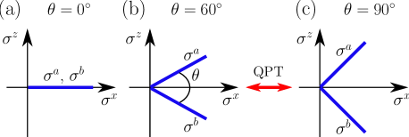
Figure 1: (Color online) Artist’s view of the evolution of orbital interactions in the generalized OCM Eq. (1) with increasing angle $\theta$. Heavy (blue) lines indicate favored spin direction induced by interactions along two nonequivalent lattice axes $a$ and $b$. Different panels show: (a) the Ising model at $\theta=0^{\circ}$, (b) the 2D $e_{g}$ orbital model at $\theta=60^{\circ}$, and (c) the OCM at $\theta=90^{\circ}$. Spin order follows the interactions in the Ising limit, while it follows one of the equivalent interactions, $\sigma^{a}$ or $\sigma^{b}$, in the OCM. This results in the symmetry breaking QPT which occurs between (b) and (c), as we show in Secs. IV-V.

Since the isotropic model has the same interaction strength for the bonds along both $a$ and $b$ axis, it is symmetric under transformation $a\leftrightarrow b$, and the issue of the QPT between different ground states of the anisotropic compass modelOru09 does not arise. On one hand, this symmetry is obeyed by the classical Ising ground state, while on the other hand, in the ground state of the OCM this symmetry is spontaneously broken (and the ground state is degenerate). Therefore, an intriguing question concerning the ground state of the model (1) is whether it has the same high symmetry as the Ising model in a broad range of $\theta$, or the symmetry is soon spontaneously broken when $\theta$ increases, i.e., there are degenerate ground states with lower symmetries, also for the $e_{g}$ orbital model, see Fig. 1(b). This question has been addressed by investigating the energy contributions along two equivalent lattice directions $a$ and $b$ by applying the MERA.

III MERA Algorithm

III.1 Calculation method

In order to obtain the ground state, we use a translationally invariant MERA on infinite lattice.Eve09 The MERA is a tensor network with infinite number of layers of disentanglers and isometries. By translational invariance, all isometries (disentanglers) in a given layer are the same. Since every layer represents a coarse-graining renormalization group transformation, shown in Fig. 2 for the 9-to-1 geometry and described in more detail in Ref. Eve09, (see their Fig. 7), we assume that after a finite number of such transformations a fixed point of the renormalization group is reached (either trivial or non-trivial) and from that time on the following transformations are the same. In other words, at the bottom of the tensor network there is a finite number of non-universal layers whose tensors are different in general, but above certain level all layers are the same. The bottom layers describe non-universal short range correlations, and the universal layers above this level describe universal properties of the fixed point. The number $N$ of the non-universal bottom layers is one of the parameters of the infinite-lattice MERA. We have verified that it is enough to keep up to three non-universal layers, depending on how close the critical point is.

Starting with randomly chosen tensors, the structure is optimized layer by layer, from the top to bottom and back. In given layer $\tau$, we calculate an environment of each tensor type by means of renormalized Hamiltonians $h_{\tau}$ and density matrices $\rho_{\tau}$ computed from other layers. The environments are aimed at updating tensors to minimize total energy. In the universal layer, this updating technique is slightly different: $h_{\infty}$ and $\rho_{\infty}$ are fixed points of the renormalization procedure defined by tensors in this layer. The above steps are iterated until the convergence of energy is achieved. For given $\theta$, we obtain the ground state for different values of bond dimension $\chi$. It turns out that in most cases it is sufficient to work with $\chi=3$, which is the same in each layer. However, it is necessary to increase $\chi$ to $4$ in the neighborhood of the critical point. The number of operations and the required memory scale as $\chi^{16}$ and $\chi^{12}$ respectively. The inset in Fig. 4(a) shows the convergence of the energy of the ground state with an increasing bond dimension. Here we also present a comparison of results obtained with the alternative 5-to-1 geometry.

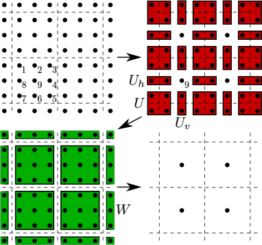
Figure 2: (Color online) 9-to-1 geometry of MERA applied to the OCM: dark (red) boxes represent the action of disentanglers $U,U_{h},U_{v}$ and gray (green) ones — isometries $W$; arrows indicate subsequent transformations used; the labels of spins 1-9 in a single block are addressed in the text. This is a coarse-graining renormalization group transformation where each $3\times 3$ plaquette in the top-left panel is replaced by a coarse grained spin in the bottom-right panel (nine spins are replaced by one coarse-grained spin). To minimize the number of states $\chi$ of the coarse-grained spin, the microscopic spins are disentangled prior to decimation. We also used a 5-to-1 geometry, see Fig. 1 of Ref. EveIsing, .

The algorithm is implemented in c++ and optimized in order to work on multi-processor computers. On an eight-core 2.3 GHz processor, it takes about half an hour to update the whole tensor network which consists of four layers of tensors with $\chi=4$. Near the critical point, i.e., at $\theta\simeq\theta_{c}$, the convergence requires several thousands of iterations whereas it is significantly faster far from $\theta_{c}$. When $\theta$ is scanned from $0^{\circ}$ to $90^{\circ}$ (or back), it is more efficient to use the previous ground state as an initial state for the next discrete value of $\theta$ instead of starting from a random initial state for each value of $\theta$. We have carefully verified convergence to the ground state by scanning $\theta$ back and forth and comparing the results with those obtained from random initial states for selected values of $\theta$.

III.2 Correlations

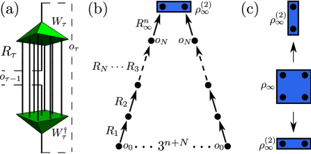
Figure 3: (Color online) (a) Renormalizer superoperator which consists of isometries only. The connections show how the isometries are contracted; compare Eq. (5). (b) Method of calculating correlations $\langle o_{\bf x}o_{\bf y}\rangle=\langle o_{0}o_{0}\rangle$ between two sites separated by a distance $3^{n+N}$. The scheme presents a graphical explanation of Eq. (9). (c) Deriving $\rho_{\infty}^{(2)}$ from $\rho_{\infty}$ when sites are separated vertically (top) and horizontally (bottom).

In order to calculate correlations, we take advantage of the special structure of the renormalization group transformation in Fig. 2. A site of the lattice that lies in the center of a $3\times 3$ decimation block (number 9 in Fig. 2) undergoes renormalization in a particularly easy manner. Since no disentangler is applied to this central site, a one-site operator $o_{\tau-1}$ at this site is mapped by the $\tau$-th renormalization group transformation to a coarse-grained one-site operator

$$o_{\tau}~{}=~{}R_{\tau}o_{\tau-1}\,.$$ (4)

Here $R_{\tau}$ is a renormalizer superoperator built out of contracted isometries only, as shown in Fig. 3(a):

$$(R_{\tau})_{kl}^{ij}~{}=~{}\sum_{n_{1},\ldots,n_{8}}(W_{\tau})^{i}_{n_{1}\ldots n_{8}k}\ (W^{\dagger}_{\tau})_{j}^{n_{1}\ldots n_{8}l}\,.$$ (5)

The meaning of the transformations $W_{\tau}$ and $W_{\tau}^{\dagger}$ is given in Figs. 2 and 3(a). Thus, if we have $N$ non-universal layers at the bottom of the geometry of MERA, then renormalized one-site operators at the central sites just below the universal layer are given by [see Fig. 3(b)]:

$$o_{N}~{}=~{}R_{N}R_{N-1}\cdots R_{1}o_{0}\,,$$ (6)

where $o_{0}\equiv o$ denotes a physical, microscopic one-site operator at one of the central sites at the very bottom of the MERA tensor network.

To extract information on the correlations, it is convenient to write eigen-decomposition of the renormalizer $R_{\infty}$ in the universal layer:

$$R_{\infty}v_{\alpha}~{}=~{}\lambda_{\alpha}v_{\alpha}\,.$$ (7)

It is straightforward to verify the basic property of the spectrum of $R_{\infty}$: $|\lambda_{\alpha}|\leq 1$. The ortonormality of the vectors $W^{i}$ in Eq. (5) implies that the identity operator $(v_{1})_{ij}=\delta_{ij}$ is an eigenvector with eigenvalue $\lambda_{1}=1$. In our numerical calculations this is the only eigenvalue with modulus $1$.

After the operator $o_{N}$ is decomposed as $o_{N}=\sum_{\alpha}o_{N}^{\alpha}v_{\alpha}$, a repeated action of the renormalizer $R_{\infty}$ in the universal layers can be written as

$$R_{\infty}^{n}o_{N}~{}=~{}\sum_{\alpha}\lambda_{\alpha}^{n}\,o_{N}^{\alpha}\,v_{\alpha}\,.$$ (8)

A correlator between two central sites ${\bf x}$ and ${\bf y}$ separated by a distance $|{\bf x}-{\bf y}|=3^{n+N}$ in the horizontal (vertical) direction is thus given by:

$$\langle o_{\bf x}o_{\bf y}\rangle = \textrm{Tr}\left\{\rho_{\infty}^{(2)}\,(R_{\infty}^{n}o_{N}\otimes R_{\infty}^{n}o_{N})\right\}$$ (9)

$$= \sum_{\alpha,\beta}o_{N}^{\alpha}o_{N}^{\beta}\,c_{\alpha\beta}\lambda_{\alpha}^{n}\lambda_{\beta}^{n}$$ (10)

$$= \sum_{\alpha,\beta}\frac{o_{N}^{\alpha}o_{N}^{\beta}\,c_{\alpha\beta}}{r^{-\log_{3}(\lambda_{\alpha}\lambda_{\beta})}}\,,$$ (11)

where $r=3^{n}$ and

$$c_{\alpha\beta}=\textrm{Tr}\left\{\rho^{(2)}_{\infty}~{}(v_{\alpha}\otimes v_{\beta})\right\}\,.$$ (12)

Here $\rho^{(2)}_{\infty}$ is a two-site reduced density matrix in a universal layer derived from $\rho_{\infty}$ as depicted in Fig. 3(c).

Correlations corresponding to the leading eigenvalue $\lambda_{1}=1$ do not decay with the distance between ${\bf x}$ and ${\bf y}$. They describe long range order in the operator $o$ and can be used to extract its expectation value $\langle o\rangle$:

$$\langle o\rangle^{2}~{}=~{}\lim_{|{\bf x}-{\bf y}|\to\infty}\langle o_{\bf x}o_{\bf y}\rangle~{}=~{}o_{N}^{1}o_{N}^{1}c_{11}~{}=~{}\left(o_{N}^{1}\right)^{2}\,,$$ (13)

where we use the property: $\lim_{n\to\infty}\lambda^{n}_{\alpha}=0$ that holds for $\alpha>1$ and the fact that $c_{11}=1$ which is a consequence of $v_{1}$ being an identity. Thus only a one-site operator with a non-zero coefficient $o_{N}^{1}$ has non-zero expectation value. A trivial example is the identity $o=\mathbb{I}$. Indeed, we obtain $o_{N}=\mathbb{I}$ in Eq. (6), which is equivalent to $o_{N}^{1}=1$, and Eq. (13) yields $\langle\mathbb{I}\rangle^{2}=1$ as expected.

IV Numerical results

IV.1 Symmetry breaking transition

Information about the ground state of the OCM Eq. (1) is contained in average energy per bond $E(\theta)$ and energy anisotropy $\Delta E(\theta)$:

$$E(\theta)\!\! = \!-\frac{1}{2}\Big{\langle}\sigma^{a}_{ij}(\theta)\sigma^{a}_{i+1,j}(\theta)+\sigma^{b}_{ij}(\theta)\sigma^{b}_{i,j+1}(\theta)\Big{\rangle},$$ (14)

$$\Delta E(\theta)\!\! = \!\Big{|}\left\langle\sigma^{a}_{ij}(\theta)\sigma^{a}_{i+1,j}(\theta)\rangle-\langle\sigma^{b}_{ij}(\theta)\sigma^{b}_{i,j+1}(\theta)\right\rangle\Big{|}.$$ (15)

In the classical limit of Ising interactions $E(0^{\circ})=-1$ and $\Delta E(0^{\circ})=0$. Due to increasing frustration, the energy $E(\theta)$ gradually increases for increasing angle $\theta$ in Eq. (1) and reaches a maximum of $E(90^{\circ})\simeq-0.57$ in the OCM, see Fig. 4(a). This increase is smooth and does not indicate the existence of a QPT.

However, by investigating the anisotropy $\Delta E(\theta)$ Eq. (15) between $a$ and $b$ bonds, we identified an angle $\theta_{c}$ at which $\Delta E(\theta)$ starts to grow. Although a gradual evolution of the ground state staring from $\theta=0^{\circ}$ might be also expected, the Ising-type state is first surprisingly robust in a broad range of angles $\theta\in[0^{\circ},\theta_{c}]$, and the energy associated with bonds along the $a$ and $b$ axes remains the same, i.e., $\Delta E(\theta)\equiv 0$. Next, the symmetry between the $a$ and $b$ directions is spontaneously broken above $\theta_{c}$, where a finite value of $\Delta E(\theta)$ is found, and then $\Delta E(\theta)$ grows rapidly with further increasing angle $\theta$, i.e., large spin correlations develop along only one of the two equivalent directions $a$ and $b$. This QPT was detected by the MERA at $\theta_{c}\simeq 84.8^{\circ}$, see Fig. 4(b).

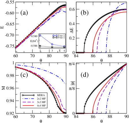
Figure 4: (Color online) Ground state obtained for the generalized OCM Eq. (1) using the MERA: (a) average energy $E$ per bond given by Eq. (14), (b) energy anisotropy $\Delta E$ given by Eq. (15), (c) spontaneous magnetization $M$ given by Eq. (17), and (d) magnetization orientation $\phi$ given by Eq. (18). Embedded $L\times L$ clusters coupled to the neighboring spins by mean-field terms ($L\times L$ MF) exhibit qualitatively similar behavior. Inset: Convergence of the ground state energy obtained by two geometries of MERA with increasing bond dimension $\chi$. Black: 9-to-1 geometry presented in Fig. 2; blue: 5-to-1 geometry introduced in Fig. 1 of Ref. EveIsing, . The 9-to-1 geometry results prove to converge faster for $\theta$ close to $\theta_{c}$.note

IV.2 Magnetization in the ground state

To understand better the QPT at $\theta_{c}$ let us consider the expectation value of the spontaneous magnetization ${\bf M}\equiv\{M^{x},M^{y},M^{z}\}$ derived from the long range order in the correlation function:

$$\lim_{|{\bf x-y}|\to\infty}\langle\sigma^{k}_{\bf x}\sigma^{l}_{{\bf y}}\rangle=M^{k}M^{l}\,,$$ (16)

where $k(l)=x,y,z$. For the interactions in Eq. (1) one finds $M^{y}\equiv 0$ for any $\theta$.

We found that the ground state obtained using the MERA for $\theta<\theta_{c}$ is characterized by $M^{z}=0$ and Ising-type long range order of $M^{x}$ which gradually decreases but remains rather large, $|M^{x}|>0.93$, in this parameter range. The symmetry between the directions $a$ and $b$ is broken above $\theta_{c}$ by appearance of a nonzero component $M^{z}$.

The value of the total magnetization

$$M=|{\bf M}|\equiv\sqrt{(M^{x})^{2}+(M^{z})^{2}}\,,$$ (17)

obtained from the MERA decreases continuously from $M(0^{\circ})=1$ in the Ising model to $M(90^{\circ})\simeq 0.92$ in the OCM, see Fig. 4(c). Thus the reduction in the order parameter $M$ by quantum fluctuations arising from the admixture of the $z$-th component, is here rather small, and reproduces qualitative results obtained for the $e_{g}$ orbital model within the linear orbital wave theory vdB99 . Furthermore, by a closer inspection of $M(\theta)$ we have found that the derivative $(\partial M(\theta)/\partial\theta)$ does not exist at $\theta=\theta_{c}$.

As expected from the behavior of $\Delta E$, the obtained symmetry breaking shown in Fig. 4 implies that the direction of spontaneous magnetization $\bf{M}$, parametrized by an orientation angle

$$\phi~{}=~{}\arctan\left(\frac{M^{z}}{M^{x}}\right)\,,$$ (18)

begins to change when $\theta$ increases above $\theta_{c}$, see Fig. 4(d). For $\theta<\theta_{c}$, the magnetization has only one component $M^{x}\neq 0$ with $\phi=0$, pointing either parallel or anti-parallel to $\sigma^{x}$ which is half-way between $\sigma^{a}(\theta)$ and $\sigma^{b}(\theta)$, see Fig. 1. Below $\theta_{c}$ the ferromagnetic ground state is doubly degenerate and the magnetization is $\pm M=\pm|M^{x}|$. When $\theta$ increases above $\theta_{c}$ the magnetization begins to rotate in the $\{M^{x},M^{z}\}$ plane by the non-zero angle $\pm\phi$ Eq. (18) with respect to the $\pm|M^{x}|$ initial magnetization below $\theta_{c}$, and each of these two states splits off into two ferromagnetic states rotated by $\pm|\phi|$ with respect to the $\sigma^{x}$-axis. As a result, one finds four degenerate states above $\theta_{c}$, and each of them is tilted with respect to $\pm\sigma^{x}$, either toward $\pm\sigma^{a}(\theta)$, or toward $\pm\sigma^{b}(\theta)$, depending on the sign of the rotation angle $\phi$. In the OCM limit $\theta=90^{\circ}$ is approached, the magnetization angle approaches $\phi=\pi/4$. In this limit there are four degenerate Ising-type ferromagnetic states, with magnetization either along $\pm\sigma^{a}(90^{\circ})$ (and $\langle\sigma^{b}(90^{\circ})\rangle=0$), or $\pm\sigma^{b}(90^{\circ})$ (and $\langle\sigma^{a}(90^{\circ})\rangle=0$).

Qualitatively the same results were obtained from the embedded $L\times L$ clusters and they are also shown in Fig. 4 for comparison. While $2\times 2$ cluster is too small and the quantum fluctuations are severely underestimated, the two larger $3\times 3$ and $4\times 4$ clusters are qualitatively similar and estimate the QPT point from above, see Fig. 4. Rather slow convergence of these results toward the MERA result for $\Delta E$ and for $|\phi|$ demonstrates the importance of longer-range correlations for the correct description of the QPT at $\theta=\theta_{c}$.

Altogether, these results show that the degenerate ground state of the generalized OCM consists of a manifold of states with broken symmetry. This confirms that the OCM is in the Ising universality class,Mis04 ; Dor05 with no quantum coupling between different broken symmetry Ising-type states. However, we found the large value of $\theta_{c}\approx 84.8^{\circ}$ rather surprising and we investigated it further using spin-wave theory. These calculations are presented in the next Section.

Another surprise is the absence of any algebraically decaying spin-spin correlations in the MERA ground state at $\theta_{c}$. They could arise from the subleading eigenvalues $\lambda_{2},\lambda_{3},\dots$ which we found to be non-zero. However, their corresponding coefficients $c_{\alpha\beta}$ with $\alpha>1$ or $\beta>1$ in Eq. (11) are small (at most $\simeq 10^{-4}$) and they decay with increasing dimension $\chi$ and especially the number of non-universal layers $N$. As a result, the only nonvanishing term in Eq. (11) is the leading one for $\alpha=\beta=1$, describing the non-decaying long range order. Notice that this observation does not exclude non-trivial short range correlations up to a distance $3^{N}$ described by the $N$ non-universal layers. We believe that when $N$ is too small, then the missing short range correlations find a way to show up in the small but non-zero universal coefficients $c_{\alpha\beta}$, but these coefficients decay quickly with increasing $N$ as the short range correlations become accurately described by the increasing number of non-universal layers.

V Spin wave expansion

Since the spin wave expansion in powers of $1/S$ becomes exact when the spin $S\to\infty$, we introduced a large-$S$ extension of the generalized OCM Hamiltonian Eq. (1) with rescaled spin operators: $\sigma^{x}\rightarrow S^{x}/S$ and $\sigma^{z}\rightarrow S^{z}/S$. We consider first the classical energy per site:

$$E_{0}(\theta,\phi)\equiv\langle{\cal H}(\theta)\rangle_{\phi}=-\frac{1}{2}\left[1+\cos\theta\cos(2\phi)\right]\,,$$ (19)

obtained using the mean-field (MF) for the ordered state of classical spins $\vec{S}$, with the magnetization direction given by Eq. (18). The classical energy has a minimum at $\phi=0$ for the entire range of $\theta\in[0^{\circ},90^{\circ})$. However, when the angle $\theta$ approaches $90^{\circ}$, the minimum becomes more and more shallow, and finally disappears completely at $\theta=90^{\circ}$. Thus, the classical ground state becomes very sensitive to quantum fluctuations in the vicinity of the maximally frustrated interactions in the OCM.

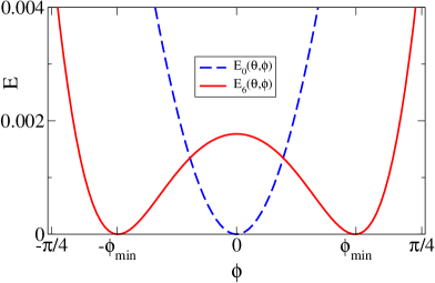
Figure 5: (Color online) Mechanism of the QPT in the generalized OCM Eq. (1) for $S=1/2$ and $\theta=87^{\circ}>\theta_{c}$. The minimum of the classical energy $E_{0}(87^{\circ},\phi)$ Eq. (19) (dashed line) at $\phi=0$ is shallow and thus unstable against weak quantum fluctuations which induce two symmetric minima at a finite value of $\pm\phi_{\rm min}$ obtained from $E_{6}(87^{\circ},\phi)$ derived from Eq. (22). For better comparison, $E_{0}$ and $E_{6}$ are shifted to have a minimum value of $0$.

This behavior of the classical ground state energy explains why small energy contributions due to quantum fluctuations may play so crucial role in the generalized OCM only in the regime of $\theta$ close to $90^{\circ}$, where they trigger a QPT by splitting the shallow symmetric classical energy minimum at $\phi=0$ into two symmetry-broken minima at finite values $\pm\phi_{\rm min}$ — we show an example of this behavior in Fig. 5 for a particular value of $\theta>\theta_{c}$. Since the quantum fluctuations induce here symmetry breaking instead of making the ground state more symmetric, this mechanism goes beyond the Landau functional paradigm.

We analyzed the effects of quantum fluctuations and the arising symmetry breaking using the Holstein-Primakoff representation of spin $\{S_{ij}^{\alpha}\}$ operators via $\{b_{ij}\}$ bosons:

$$\!\!\cos\phi~{}S^{x}_{ij}+\sin\phi~{}S^{z}_{ij}\!\! = \!S-b_{ij}^{\dagger}b_{ij}\,,$$ (20)

$$\!\!-\sin\phi~{}S^{x}_{ij}+\cos\phi~{}S^{z}_{ij}\!\! = \!\frac{b_{ij}^{\dagger}}{2}\sqrt{2S-b_{ij}^{\dagger}b_{ij}}+\mathrm{H.c.}\,.$$ (21)

Operators $\{b_{ij},b_{ij}^{\dagger}\}$ satisfy standard bosonic commutation relations: $[b_{ij},b_{i^{\prime}j^{\prime}}]=0$ and $[b_{ij},b_{i^{\prime}j^{\prime}}^{\dagger}]=\delta_{ii^{\prime}}\delta_{jj^{\prime}}$. In this approach, we are looking for a critical value $\theta_{c}$, above which it is energetically favorable to change the direction of magnetization $\bf{M}$ from the symmetric state $\phi=0$ to a symmetry-broken state with a finite value of $\phi\neq 0$. We expanded the square root in Eq. (21) in powers of $1/(2S)$ and obtained an expansion of Hamiltonian Eq. (1) in powers of the operators $\{b_{ij},b_{ij}^{\dagger}\}$. As we applied Wick’s theorem to reduce the obtained Hamiltonian to an effective quadratic Hamiltonian, the terms proportional to the odd powers of $1/(2S)$ do not contribute and are skipped below (for more details see the Appendix). When truncated at the sixth order term this expansion reads

$$\widetilde{H}_{6}\simeq H_{0}+(2S)^{-1}H_{2}+(2S)^{-2}H_{4}+(2S)^{-3}H_{6}\,.$$ (22)

Here $H_{2n}$ is a sum of all terms of the $2n$-th order in $\{b_{ij},b_{ij}^{\dagger}\}$ operators. In a similar way, $\widetilde{H}_{4}$ and $\widetilde{H}_{2}$ denote expansions truncated at the fourth and second order terms, respectively. We have found a posteriori that the second order expansion $\widetilde{H}_{2}$ (noninteracting spin waves) does not suffice and higher order terms are necessary. Consequently, we consider below Hamiltonian Eq. (1) expanded up to the sixth order.

For given $\theta$ and $\phi$, we can approximate the ground state of the boson Hamiltonian given by Eq. (22) by a Bogoliubov vacuum obtained as the ground state of the quadratic Hamiltonian $\widetilde{H}^{\rm MF}_{2}$ obtained using the MF averaging of four- and six-boson terms. Details of this calculation can be found in the Appendix A.

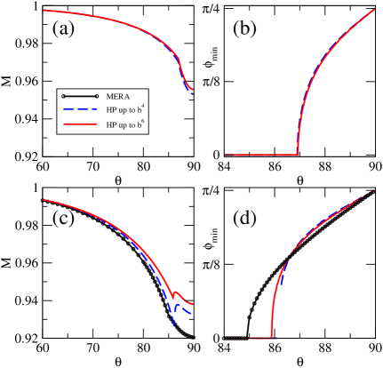
Figure 6: (Color online) Symmetry breaking in the ground state as obtained from the boson expansion Eq. (22). Panels (a) and (b) show results for $S=1$, (c) and (d) — for $S=1/2$; (a) and (c) depict magnetization $M$ Eq. (17), (b) and (d) — the value of the magnetization angle $\phi$ Eq. (18) that minimizes energy. Calculations for $\widetilde{H}_{6}$ predict the following values of $\theta_{c}$: $85.89^{\circ}$, $86.9^{\circ}$, $88.2^{\circ}$, and $89.2^{\circ}$ for $S=1/2$, $S=1$, $S=2$, and $S=5$, respectively (the last two not shown), and $\theta_{c}\to 90^{\circ}$ for $S\to\infty$.

First we performed separate calculations for $\widetilde{H}_{2}$, $\widetilde{H}_{4}$ and $\widetilde{H}_{6}$ for several values of spin $S\geq 1$ when the $1/(2S)$-expansion given in Eq. (22) is convergent. The quadratic $\widetilde{H}_{2}$ fails for large $\theta$, where its spectrum becomes gapless and the magnetization $M$ Eq. (17) diverges. In contrast, $\widetilde{H}_{4}$ and $\widetilde{H}_{6}$ give only small reduction in $M$ in the entire range of $\theta$, see Fig. 6(a) and 6(c). Interestingly, the Bogoliubov spectrum remains gapful at $\theta_{c}$ in both the fourth and sixth order expansions and, just like in the MERA, there are no algebraically decaying spin-spin correlations. The critical angle $\theta_{c}$ at which the symmetry-breaking QPT occurs increases toward $90^{\circ}$ with increasing $S$ when the quantum fluctuations become less significant. Therefore, the magnetization $M$ increases with increasing $S$ and it tends to $1$ in the classical limit $S\to\infty$.

Encouraged by these results, we also performed similar calculations for the generalized OCM Eq. (1) with $S=1/2$, where the convergence of the $1/(2S)$-expansion becomes problematic. Unlike for $S\geq 1$, we find that the fourth order expansion is insufficient as it predicts the first order QPT [Fig. 6(d)] and does not agree qualitatively with the prediction of the MERA, see Sec. IV. Only in the sixth order one finds a qualitative agreement between the present boson expansion and the MERA, both giving the second order QPT at $\theta_{c}$. A cusp in $M(\theta)$ seen in Fig. 6(c) shows that even the sixth order expansion is not quite converged for $S=1/2$. Again, the Bogoliubov spectrum remains gapful at $\theta_{c}$ in the sixth order expansion, with a finite gap equal $1.52$, and one finds no algebraically decaying spin-spin correlations.

VI Conclusions

Summarizing, we found that a second order quantum phase transition in the generalized orbital compass model Eq. (1) occurs at $\theta_{c}=84.8^{\circ}$ which is surprisingly close to the compass point $\theta=90^{\circ}$, i.e., only when the interactions are sufficiently strongly frustrated. There is spontaneous ferromagnetic magnetization at any angle $\theta\in[0^{\circ},90^{\circ}]$. Below $\theta_{c}$ the ferromagnetic ground state is doubly degenerate with the spontaneous magnetization, either parallel or antiparallel to the average direction $\sigma^{a}_{ij}+\sigma^{b}_{ij}$. None of the directions, neither $a$ nor $b$, is preferred in this symmetric phase. In contrast, when $\theta$ increases above $\theta_{c}$ the symmetry between $a$ and $b$ becomes spontaneously broken and the ferromagnetic magnetization begins to align parallel/antiparallel to either $\sigma^{a}_{ij}$ or $\sigma^{b}_{ij}$. The ground state is fourfold degenerate in this symmetry-broken phase. The spontaneous magnetization $M$ is close to $1$ and quantum fluctuations remain small in the whole range of $\theta\in(0^{\circ},90^{\circ}]$.

These results were obtained using the MERA and the mechanism of the QPT was explained within the spin-wave theory. For classical spins the minimum of energy is at one of the two symmetric states with the magnetization either parallel or antiparallel to $\sigma^{a}_{ij}+\sigma^{b}_{ij}$, see Fig. 5. The minimum becomes more and more shallow as the compass point $\theta=90^{\circ}$ is approached. However, the quantum fluctuations are weak due to the gapful orbital wave excitations, and only very close to the above OCM point become strong enough to split the shallow minimum into two distinct minima in the vicinity of the OCM point. In this way the symmetry between the axes $a$ and $b$ is spontaneously broken. For this reason the orbital $e_{g}$ model with ferro-orbital interactions, considered in Ref. vdB99, and corresponding to a “moderate” value of $\theta=60^{\circ}$ [see Fig. 1(b)], orders in a symmetric (uniform) phase induced by the stronger (here $\propto\sigma^{x}_{ij}\sigma^{x}_{i^{\prime}j^{\prime}}$) interaction component.

Interestingly, since — unlike in the Landau paradigm — the symmetry in the present model Eq. (1) is broken rather than restored by quantum fluctuations, we do not find any algebraically decaying spin-spin correlations at the critical point found in the generalized orbital compass model Eq. (1). The spin waves also remain gapful at this point.

Appendix A Details of the spin wave calculation

In this section we present the details of the spin wave calculation. We consider the general case of an $L\times L$ square lattice, with $L$ being odd for convenience. The results presented in Section V are obtained after taking the thermodynamic limit $L\to\infty$.

For given $\theta$ and $\phi$, the ground state of the boson Hamiltonian Eq. (22) is approximated by a Bogoliubov vacuum obtained as the ground state of a mean-field (MF) quadratic Hamiltonian $\widetilde{H}^{\rm MF}_{2}$ (to be derived later on). Terms $H_{2}$, $H_{4}$ and $H_{6}$ in Eq. (22) are given by:

$$H_{2}~{}=~{}4[1+\cos\theta\cos(2\phi)]\sum_{\bf r}b^{\dagger}_{\bf r}b_{\bf r}\\ -\sin^{2}\left(\phi-\frac{\theta}{2}\right)\sum_{\bf r}\left(b^{\dagger}_{\bf r}b_{{\bf r}+{\bf e_{x}}}+b_{\bf r}b_{{\bf r}+{\bf e_{x}}}+\mathrm{H.c.}\right)\\ -\sin^{2}\left(\phi+\frac{\theta}{2}\right)\sum_{\bf r}\left(b^{\dagger}_{\bf r}b_{{\bf r}+{\bf e_{y}}}+b_{\bf r}b_{{\bf r}+{\bf e_{y}}}+\mathrm{H.c.}\right)\,,$$ (23)

$$H_{4}~{}=~{}-4\cos^{2}\left(\phi-\frac{\theta}{2}\right)\sum_{\bf r}b^{\dagger}_{\bf r}b^{\dagger}_{{\bf r}+{\bf e_{x}}}b_{\bf r}b_{{\bf r}+{\bf e_{x}}}\\ -4\cos^{2}\left(\phi+\frac{\theta}{2}\right)\sum_{\bf r}b^{\dagger}_{\bf r}b^{\dagger}_{{\bf r}+{\bf e_{y}}}b_{\bf r}b_{{\bf r}+{\bf e_{y}}}\\ +\frac{1}{2}\sin^{2}\left(\phi-\frac{\theta}{2}\right)\sum_{\bf r}\left\{b^{\dagger}_{\bf r}b_{\bf r}^{2}(b_{{\bf r}\pm{\bf e_{x}}}+b^{\dagger}_{{\bf r}\pm{\bf e_{x}}})+\mathrm{H.c.}\right\}\\ +\frac{1}{2}\sin^{2}\left(\phi+\frac{\theta}{2}\right)\sum_{\bf r}\left\{b^{\dagger}_{\bf r}b_{\bf r}^{2}(b_{{\bf r}\pm{\bf e_{y}}}+b^{\dagger}_{{\bf r}\pm{\bf e_{y}}})+\mathrm{H.c.}\right\}\,,$$ (24)

$$H_{6}~{}=~{}\frac{1}{8}\sin^{2}\left(\phi-\frac{\theta}{2}\right)\sum_{\bf r}\left\{\left(b^{\dagger}_{\bf r}b_{\bf r}\right)^{2}b_{\bf r}(b_{{\bf r}\pm{\bf e_{x}}}+b^{\dagger}_{{\bf r}\pm{\bf e_{x}}})\right.\\ \left.-~{}2b^{\dagger}_{\bf r}b^{\dagger}_{{\bf r}+{\bf e_{x}}}b_{\bf r}^{2}(b_{{\bf r}+{\bf e_{x}}}+b^{\dagger}_{{\bf r}+{\bf e_{x}}})b_{{\bf r}+{\bf e_{x}}}+\mathrm{H.c.}\right\}\\ +\frac{1}{8}\sin^{2}\left(\phi+\frac{\theta}{2}\right)\sum_{\bf r}\left\{\left(b^{\dagger}_{\bf r}b_{\bf r}\right)^{2}b_{\bf r}(b_{{\bf r}\pm{\bf e_{y}}}+b^{\dagger}_{{\bf r}\pm{\bf e_{y}}})\right.\\ \left.-~{}2b^{\dagger}_{\bf r}b^{\dagger}_{{\bf r}+{\bf e_{y}}}b_{\bf r}^{2}(b_{{\bf r}+{\bf e_{y}}}+b^{\dagger}_{{\bf r}+{\bf e_{y}}})b_{{\bf r}+{\bf e_{y}}}+\mathrm{H.c.}\right\}\,,$$ (25)

where ${\bf r}=(i,j)$, ${\bf e_{x}}=(1,0)$ and ${\bf e_{y}}=(0,1)$. The $\pm$ signs mean here that both terms, with $+$ and $-$ sign separately, must be taken into account.

To derive the quadratic approximation $\widetilde{H}^{\rm MF}_{2}$, we replace the boson terms in $H_{4}$ and $H_{6}$ with two-boson terms and proper averages by means of the MF approximation and Wick’s theorem. This justifies a posteriori why the expansion (22) is limited only to the terms with even number of boson operators. As an example of this approximation, consider one of the contributions to $H_{4}$ in Eq. (24): $b_{\bf r}^{\dagger}b_{\bf r}^{2}b_{{\bf r}+{\bf e_{x}}}$, which is replaced with a quadratic term:

$$b_{\bf r}^{\dagger}b_{\bf r}^{2}b_{{\bf r}+{\bf e_{x}}}~{}\simeq~{}2\langle b_{\bf r}^{\dagger}b_{\bf r}\rangle\;b_{\bf r}b_{{\bf r}+{\bf e_{x}}}+2\langle b_{\bf r}b_{{\bf r}+{\bf e_{x}}}\rangle\;b_{\bf r}^{\dagger}b_{{\bf r}}\\ +\langle b_{\bf r}^{\dagger}b_{{\bf r}+{\bf e_{x}}}\rangle\;b_{\bf r}^{2}+\langle b_{\bf r}^{2}\rangle\;b_{\bf r}^{\dagger}b_{{\bf r}+{\bf e_{x}}}-\langle b_{\bf r}^{\dagger}b_{\bf r}^{2}b_{{\bf r}+{\bf e_{x}}}\rangle\,.$$ (26)

The above replacement procedure leads to six MF parameters $\{m_{i}\}\equiv\{m_{1},m_{2},\ldots,m_{6}\}$ that should satisfy self-consistency conditions. These are in fact all possible combinations of operators defined on nearest-neighbor sites that cannot be derived one from another by commutation relations and translational invariance of the lattice, i.e., $m_{1}=\langle b^{\dagger}_{\bf r}b_{\bf r}\rangle$, $m_{2}=\langle b^{\dagger}_{\bf r}b_{{\bf r}+{\bf e_{x}}}\rangle$, $m_{3}=\langle b^{\dagger}_{\bf r}b_{{\bf r}+{\bf e_{y}}}\rangle$, $m_{4}=\langle b_{\bf r}^{2}\rangle$, $m_{5}=\langle b_{\bf r}b_{{\bf r}+{\bf e_{x}}}\rangle$, and $m_{6}=\langle b_{\bf r}b_{{\bf r}+{\bf e_{y}}}\rangle$.

The obtained Hamiltonian $\widetilde{H}^{\rm MF}_{2}$ is diagonalized by the Fourier transformation followed by the Bogoliubov transformation. Fourier transformation which is consistent with periodic boundary conditions $b_{L+1,j}=b_{1,j}$ and $b_{i,L+1}=b_{i,1}$ has the following form:

$$b_{\bf r}~{}=~{}\frac{1}{L}\sum_{\bf k}b_{\bf k}\>e^{i\,{\bf k}\cdot{\bf r}}\,,$$ (27)

where ${\bf k}=(k_{x},k_{y})$ is the momentum. In the sum, momentum components $k_{x}$ and $k_{y}$ take the values (for odd $L$ considered here):

$$k_{x(y)}~{}=~{}0\cdot\frac{2\pi}{L},\;\pm 1\cdot\frac{2\pi}{L},\;\ldots,\;\pm\frac{L-1}{2}\cdot\frac{2\pi}{L}\,.$$ (28)

Diagonalization of $\widetilde{H}^{\rm MF}_{2}$ is completed by the Bogoliubov transformation:

$$b_{\bf k}~{}=~{}u_{\bf k}\gamma_{\bf k}+v_{-\bf k}^{\ast}\gamma_{-\bf k}^{\dagger}\,,$$ (29)

where the modes $u_{\bf k}$ and $v_{\bf k}$ are normalized such that $|u_{\bf k}|^{2}-|v_{\bf k}|^{2}=1$. The obtained modes are used to calculate new values of the MF parameters $\{m_{i}\}$ ($i=1,2,\ldots,6$). For instance, one of them reads: $m_{2}=\langle b^{\dagger}_{\bf r}b_{{\bf r}+{\bf e_{x}}}\rangle=\frac{1}{L^{2}}\sum_{\bf k}|v_{\bf k}|^{2}\cos k_{x}$. Starting from random values, the above steps are iteratively applied until full convergence of all $\{m_{i}\}$ is reached, which results in satisfying the self-consistency conditions.

References

- (1) Y. Tokura and N. Nagaosa, Science 288, 462 (2000); A. Weiße and H. Fehske, New J. Phys. 6, 158 (2004); E. Dagotto, ibid. 7, 67 (2005).
- (2) P. Horsch, A. M. Oleś, L. F. Feiner, and G. Khaliullin, Phys. Rev. Lett. 100, 167205 (2008); A. M. Oleś and P. Horsch, in: Properties and Applications of Thermoelectric Materials — The Search for New Materials for Thermoelectric Devices, ed. V. Zlatic and A. C. Hewson (Springer, New York, 2009), p. 299; A. M. Oleś, Acta Phys. Pol. A 115, 36 (2009).
- (3) L. F. Feiner, A. M. Oleś and J. Zaanen, Phys. Rev. Lett. 78, 2799 (1997).
- (4) K. I. Kugel and D. I. Khomskii, Sov. Phys. Usp. 25, 231 (1982); D. I. Khomskii and M. V. Mostovoy, J. Phys. A 36, 9197 (2003).
- (5) Z. Nussinov, M. Biskup, L. Chayes, and J. van den Brink, Europhys. Lett. 67, 990 (2004).
- (6) A. Mishra, M. Ma, F.-C. Zhang, S. Guertler, L.-H. Tang, and S. Wan, Phys. Rev. Lett. 93, 207201 (2004).
- (7) J. Dorier, F. Becca, and F. Mila, Phys. Rev. B72, 024448 (2005); S. Wenzel and W. Janke, ibid. 78, 064402 (2008).
- (8) B. Douçot, M. V. Feigel’man, L. B. Ioffe, and A. S. Ioselevich, Phys. Rev. B71, 024505 (2005); Z. Nussinov and E. Fradkin, ibid. 71, 195120 (2005).
- (9) G. Jackeli and G. Khaliullin, Phys. Rev. Lett. 102, 017205 (2009).
- (10) A. Nagano, M. Naka, J. Nasu, and S. Ishihara, Phys. Rev. Lett. 99, 217202 (2007).
- (11) A. Kitaev, Ann. Phys. (N.Y.) 321, 2 (2006).
- (12) Z. Nussinov and G. Ortiz, Ann. Phys. (N.Y.) 324, 977 (2009).
- (13) P. Milman, W. Maineult, S. Guibal, L. Guidoni, B. Douçot, L. Ioffe, and T. Coudreau, Phys. Rev. Lett. 99, 020503 (2007).
- (14) W. Brzezicki, J. Dziarmaga, and A. M. Oleś, Phys. Rev. B75, 134415 (2007); E. Eriksson and H. Johannesson, ibid. 79, 224424 (2009).
- (15) R. Orús, A. C. Doherty, and G. Vidal, Phys. Rev. Lett. 102, 077203 (2009).
- (16) G. Vidal, Phys. Rev. Lett. 99, 220405 (2007).
- (17) G. Vidal, Phys. Rev. Lett. 101, 110501 (2008).
- (18) S. Sachdev, Quantum Phase Transitions (Cambridge University Press, Cambridge, U.K., 1999).
- (19) S. R. White, Phys. Rev. Lett. 69, 2863 (1992); Phys. Rev. B48, 10345 (1993).
- (20) K. Hallberg, Adv. Phys. 55, 477 (2006).
- (21) L. Cincio, J. Dziarmaga, and M. M. Rams, Phys. Rev. Lett. 100, 240603 (2008).
- (22) G. Evenbly and G. Vidal, Phys. Rev. Lett. 102, 180406 (2009).
- (23) G. Evenbly and G. Vidal, Phys. Rev. B79, 144108 (2009).
- (24) V. Giovannetti, S. Montangero, and R. Fazio, Phys. Rev. Lett. 101, 180503 (2008); V. Giovannetti, S. Montangero, M. Rizzi, and R. Fazio, Phys. Rev. A79, 052314 (2009); S. Montangero, M. Rizzi, V. Giovannetti, and R. Fazio, Phys. Rev. B80, 113103 (2009); P. Silvi, V. Giovannetti, P. Calabrese, G. E. Santoro, and R. Fazio, J. Stat. Mech. L03001 (2010).
- (25) C. M. Dawson, J. Eisert, and T. J. Osborne, Phys. Rev. Lett. 100, 130501 (2008).
- (26) T. Barthel, C. Pineda, and J. Eisert, Phys. Rev. A80, 042333 (2009); C. Pineda, T. Barthel, and J. Eisert, Phys. Rev. A81, 050303 (2010).
- (27) G. Evenbly and G. Vidal, Phys. Rev. B81, 235102 (2010).
- (28) G. Evenbly and G. Vidal, Phys. Rev. Lett. 104, 187203 (2010).
- (29) The orbital interactions in transition metal oxides favor alternating orbital order, see Refs. Tok00, ; Hor08, — the corresponding OCM is equivalent to the present ferro-orbital model Eq. (1) by a unitary transformation.
- (30) L. F. Feiner and A. M. Oleś, Phys. Rev. B59, 3295 (1999).
- (31) J. van den Brink, P. Horsch, F. Mack, and A. M. Oleś, Phys. Rev. B59, 6795 (1999).
- (32) The comparison has been made for geometries with the same bond dimension in all layers. The performance of 5-to-1 geometry can be further improved by considering different bond dimensions on some indices.