Abstract

The top quark has a large Yukawa coupling with the Higgs boson. In the usual extensions of the standard model the Higgs sector includes extra scalars, which also tend to couple strongly with the top quark. Unlike the Higgs, these fields have a natural mass above $2m_{t}$, so they could introduce anomalies in $t\bar{t}$ production at the LHC. We study their effect on the $t\bar{t}$ invariant mass distribution at $\sqrt{s}=7$ TeV. We focus on the bosons ($H$,$A$) of the minimal SUSY model and on the scalar field ($r$) associated to the new scale $f$ in Little Higgs (LH) models. We show that in all cases the interference with the standard amplitude dominates over the narrow-width contribution. As a consequence, the mass difference between $H$ and $A$ or the contribution of an extra $T$-quark loop in LH models become important effects in order to determine if these fields are observable there. We find that a 1 fb^-1 luminosity could probe the region $\tan\beta\leq 3$ of SUSY and $v/(\sqrt{2}f)\geq 0.3$ in LH models.

1 Introduction

The main objective of the LHC is to reveal the nature of the mechanism breaking the electroweak (EW) symmetry. This requires not only a determination of the Higgs mass and couplings, but also a search for additional particles that may be related to new dynamics or symmetries present at the TeV scale. The top-quark sector appears then as a promising place to start the search, as it is there where the EW symmetry is broken the most (it contains the heaviest fermion). Generically, the large top-quark Yukawa coupling with the Higgs boson ($h$) also implies large couplings with the extra physics. For example, in SUSY extensions $h$ comes together with neutral scalar ($H$) and pseudoscalar ($A$) fields [1]. Or in Little Higgs (LH) models, a global symmetry in the Higgs and the top-quark sectors introduces a scalar singlet and an extra $T$ quark [2, 3]. In all cases these scalar fields have large Yukawa couplings that could imply a sizeable production rate in hadron collisions and a dominant decay channel into $t\bar{t}$.

The energy and the luminosity to be achieved at the LHC make this collider a top-quark factory, with around $1.5\times 10^{5}$ pairs at $\sqrt{s}=7$ TeV and 1 fb^-1. In this paper we study the possibility that the production and decay of extra Higgses distorts the $t\bar{t}$ invariant mass distribution ($m_{t\bar{t}}$). The relevant amplitudes are pictured in Fig. 1. We first review [4, 5] the (analytical) expressions for the cross section when the intermediate field is a scalar or a pseudoscalar field and the loop fermion is the top or a heavier $T$ quark. Then we define the models to be analyzed and study the parton-level cross section in each case. Finally we discuss the possible signal at the LHC.

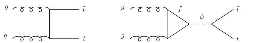
Figure 1: Diagrams that interfere in $t\bar{t}$ production.

2 Top quarks from scalar Higgs bosons

The potential to observe new physics in $m_{t\bar{t}}$ at hadron colliders has been discussed in previous literature [5, 6, 7, 8, 9, 10, 11, 12, 13]. In general, any heavy $s$–channel resonance with a significant branching ratio to $t\bar{t}$ will introduce distortions: a bump that can be evaluated in the narrow-width approximation or more complex structures (a peak followed by a dip) when interference effects are important [14]. In the diagram depicted in Fig. 1 the intermediate scalar is produced at one loop [15], but the gauge and Yukawa couplings are all strong.

Let us first consider a scalar $\phi$ coupled to the top quark and (possibly) to a heavy fermion. The leading-order (LO) differential cross section for $gg\rightarrow t\bar{t}$ is then

$${{\rm d}\sigma\over{\rm d}z} = {{\rm d}\sigma_{QCD}\over{\rm d}z}+{\alpha_{s}^{2}\;y_{\phi\bar{t}t}^{2}\;s^{2}\;\beta^{3}\over 1536\;\pi^{3}}\;\left|{N(s)\over s-m_{\phi}^{2}+i\;m_{\phi}\Gamma_{\phi}(s)}\right|^{2}$$ (2)

$$-{\alpha_{s}^{2}\;y_{\phi\bar{t}t}\;m_{t}\;\beta^{3}\over 48\sqrt{2}\;\pi}\;{1\over 1-\beta^{2}z^{2}}\;{\rm Re}\left[{N(s)\over s-m_{\phi}^{2}+i\;m_{\phi}\Gamma_{\phi}(s)}\right]\;,$$

where $z=\cos\theta$ is the cosine of the angle between an incoming $g$ and $t$, $m_{t}$ and $y_{\phi\bar{t}t}$ are the top-quark mass and Yukawa coupling, and $\beta=\sqrt{1-4m_{t}^{2}/s}$ is the velocity of $t$ in the center of mass frame. The function $N(s)$ associated to the fermion loop is

$$N(s)=\sum_{f}{3\;m_{f}\;y_{\phi\bar{f}f}\over\sqrt{2}\;s}\left[1+\left(1-{4m_{f}^{2}\over s}\right)I_{f}(s)\right]\;,$$ (3)

where $f$ may be the top or another quark strongly coupled to $\phi$, and $I_{f}(s)$ takes a different form depending on the mass $m_{f}$:

$$I_{f}(s)=\left\{\begin{array}[]{l l}\displaystyle\left({\rm Arcsin}\sqrt{s\over 4m_{f}^{2}}\right)^{2}&s<4m_{f}^{2}\;;\\ \\ \displaystyle-{1\over 4}\left(\ln{1+\sqrt{1-4m_{f}^{2}/s}\over 1-\sqrt{1-4m_{f}^{2}/s}}-i\;\pi\right)^{2}&s>4m_{f}^{2}\;.\end{array}\right.$$ (4)

If $2m_{f}>\sqrt{s}$ then $I_{f}$ is real and the interference vanishes at $s=m_{\phi}^{2}$. If $f$ is the top or any fermion with $2m_{f}<\sqrt{s}$, then this contribution can be seen as a final-state $f\bar{f}$ interaction [5]. The diferential QCD contribution ${\rm d}\sigma_{QCD}/{\rm d}z$ can be found in [16, 17].

For a pseudoscalar $A$ we have

$${{\rm d}\sigma\over{\rm d}z} = {{\rm d}\sigma_{QCD}\over{\rm d}z}+{3\;\alpha_{s}^{2}\;y_{A\bar{t}t}^{2}\;s^{2}\;\beta\over 512\;\pi^{3}}\;\left|{P(s)\over s-m_{A}^{2}+i\;m_{A}\Gamma_{A}(s)}\right|^{2}$$ (6)

$$-{\alpha_{s}^{2}\;y_{A\bar{t}t}\;m_{t}\;\beta\over 16\sqrt{2}\;\pi}\;{1\over 1-\beta^{2}z^{2}}\;{\rm Re}\left[{P(s)\over s-m_{A}^{2}+i\;m_{A}\Gamma_{A}(s)}\right]\;,$$

with

$$P(s)=\sum_{f}{m_{f}\;y_{A\bar{f}f}\over\sqrt{2}\;s}\;I_{f}(s)\;.$$ (7)

As we will see in the next section, to have an observable effect it is essential that the width $\Gamma_{\phi}$ is small. This is precisely the reason why the effect on $m_{t\bar{t}}$ of a very heavy standard Higgs $h$ would be irrelevant. A 500 GeV Higgs boson would couple strongly to the top quark, but even stronger to itself: $\lambda=m_{h}^{2}/(2v^{2})\approx 2$. Its decay into would-be Goldstone bosons (eaten by the massive $W$ and $Z$) would then dominate, implying a total decay width

$$\Gamma_{h}\approx{3\over 8\pi\;v^{2}}\left[{m_{t}^{2}m_{h}\;\beta_{t}^{3}}+{m_{h}^{3}\over 4}\left(\beta_{V}^{3}+{3\over 4}\beta_{V}(1-\beta_{V}^{2})^{2}\right)\right]\;\approx 60\;{\rm GeV}\;,$$ (8)

where

$$\beta_{t(V)}=\sqrt{1-{4m_{t(V)}^{2}\over m_{h}^{2}}}\;$$ (9)

and we have taken a common $W,Z$ mass $m_{V}\approx 90$ GeV.

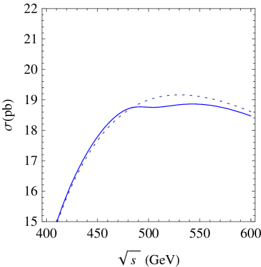
Figure 2: $\sigma(gg\rightarrow t\bar{t})$ with a standard Higgs of mass $m_{h}=500$ GeV.

The plot in Fig. 2 shows a too small deviation due to the standard Higgs in $\sigma(gg\rightarrow t\bar{t})$. To have a smaller width and a larger effect the mass of the resonance must not be EW. In particular, SUSY or LH models provide a new scale and massive Higgses with no need for large scalar self-couplings.

3 SUSY neutral bosons

SUSY incorporates two Higgs doublets, and after EW symmetry breaking there are two neutral bosons ($H$ and $A$) in addition to the light Higgs. The mass of these two fields is not EW (it comes from the SUSY breaking sector), so they are naturally heavy enough to decay in $t\bar{t}$. Their mass difference is EW, of order $M_{Z}^{2}/m_{A}$, with important top-quark corrections at the loop level. More precisely, the relation between $m_{A}$ and $m_{H,h}$ is [18]

$$m_{H,h}^{2}={1\over 2}\left(m_{A}^{2}+M_{Z}^{2}+\Delta_{11}+\Delta_{22}\pm\sqrt{\Delta_{0}^{2}}\right)$$ (10)

where

$$\Delta_{0}^{2} = \left(m_{A}^{2}+M_{Z}^{2}+\Delta_{11}+\Delta_{22}\right)^{2}-4\;m_{A}^{2}M_{Z}^{2}\cos^{2}2\beta$$ (11)

$$-4\left(\Delta_{11}\Delta_{22}-\Delta_{12}^{2}\right)-4\left(M_{Z}^{2}\cos^{2}\beta+m_{A}^{2}\sin^{2}\beta\right)\Delta_{22}$$

$$-4\left(M_{Z}^{2}\sin^{2}\beta+m_{A}^{2}\cos^{2}\beta\right)\Delta_{11}-4\;\sin 2\beta\left(M_{Z}^{2}+m_{A}^{2}\right)\Delta_{12}\;,$$

$$\Delta_{11} = {3g^{2}\over 16\pi^{2}}\;{m_{t}^{4}\over M_{W}^{2}\sin^{2}\beta}\left[{\mu\left(A_{t}m_{0}-\mu\cot\beta\right)\over\tilde{m}_{t1}^{2}-\tilde{m}_{t2}^{2}}\right]^{2}d(\tilde{m}_{t1}^{2},\tilde{m}_{t2}^{2})\;,$$ (12)

$$\Delta_{22} = {3g^{2}\over 16\pi^{2}}\;{m_{t}^{4}\over M_{W}^{2}\sin^{2}\beta}\;\Bigg{[}\;{2A_{t}m_{0}\left(A_{t}m_{0}-\mu\cot\beta\right)\over\tilde{m}_{t1}^{2}-\tilde{m}_{t2}^{2}}\;\ln{\tilde{m}_{t1}^{2}\over\tilde{m}_{t2}^{2}}$$ (13)

$$+\ln{\tilde{m}_{t1}^{2}\tilde{m}_{t2}^{2}\over m_{t}^{4}}+\left({A_{t}m_{0}\left(A_{t}m_{0}-\mu\cot\beta\right)\over\tilde{m}_{t1}^{2}-\tilde{m}_{t2}^{2}}\right)^{2}d(\tilde{m}_{t1}^{2},\tilde{m}_{t2}^{2})\;\Bigg{]}\;,$$

$$\Delta_{12} = -{3g^{2}\over 16\pi^{2}}\;{m_{t}^{4}\over M_{W}^{2}\sin^{2}\beta}\;{\mu\left(A_{t}m_{0}-\mu\cot\beta\right)\over\tilde{m}_{t1}^{2}-\tilde{m}_{t2}^{2}}\;\Bigg{[}\;\ln{\tilde{m}_{t1}^{2}\over\tilde{m}_{t2}^{2}}$$ (14)

$$+{A_{t}m_{0}\left(A_{t}m_{0}-\mu\cot\beta\right)\over\tilde{m}_{t1}^{2}-\tilde{m}_{t2}^{2}}\;d(\tilde{m}_{t1}^{2},\tilde{m}_{t2}^{2})\;\Bigg{]}\;,$$

and

$$d(m_{1}^{2},m_{2}^{2})=2-{m_{1}^{2}+m_{2}^{2}\over m_{1}^{2}-m_{2}^{2}}\;\ln{m_{1}^{2}\over m_{2}^{2}}\;.$$ (15)

Varying the $\mu$ parameter and the stop masses and trilinears, for $m_{A}=500$ GeV we obtain typical values of $m_{H}-m_{A}$ between $-2$ and $+10$ GeV.

The scalar masses of interest correspond to the decoupling regime, where $h$ is basically the SM Higgs and

$$y_{H\bar{t}t}\approx-{m_{t}\sqrt{2}\over v}\;{1\over\tan\beta}\approx-y_{A\bar{t}t}\;.$$ (16)

In addition, we will consider low values of $\tan\beta$, where the decay into bottom quarks is not important and the (energy-dependent) widths can be approximated to

$$\Gamma_{H}(s)\approx{3\;y_{H\bar{t}t}^{2}\;s\;\beta^{3}\over 16\pi\;m_{H}}\;,\;\;\;\Gamma_{A}(s)\approx{3\;y_{A\bar{t}t}^{2}\;s\;\beta\over 16\pi\;m_{A}}\;.$$ (17)

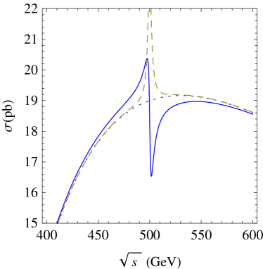
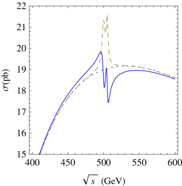
Figure 3: $\sigma(gg\rightarrow t\bar{t})$ for $\tan\beta=2$ and SUSY bosons of mass $m_{A}=m_{H}=500$ GeV (left) or $m_{A}=500$, $m_{H}=505$ GeV (right). Dashes provide the narrow-width approximation and dots the standard model cross section.

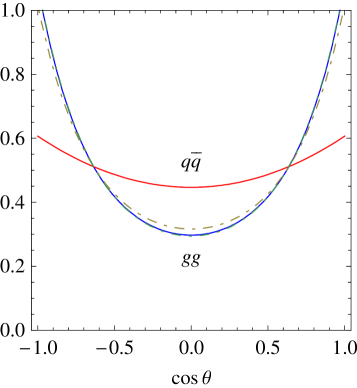
Figure 4: Standard angular distribution for the $t$ quarks from $q\bar{q}$ and $gg$ collisions at $\sqrt{s}=500$ GeV. We include (dashes) the distribution from $gg$ at the peak and the dip of Fig. 3–left.

In Fig. 3 we plot $\sigma(gg\rightarrow t\bar{t})$ at center of mass energies around $m_{A}=500$ GeV for $m_{H}=500$ GeV (left) and $m_{H}=505$ GeV (right). We have taken $\tan\beta=2$, which implies $\Gamma_{H}\approx 3.0$ GeV and $\Gamma_{A}\approx 5.3$ GeV. We observe an average 5.5% excess and 8.1% deficit in the 5 GeV intervals before and after $\sqrt{s}=500$ GeV, respectively. We include in dashes the result ignoring the interference (last term in Eqs. (2) and (6)), which would not be captured if one uses the narrow-width approximation. It is apparent that the interference with the standard amplitude gives the dominant effect. In Fig. 3–left the position of the peaks and dips caused by $H$ and $A$ overlap constructively (notice, however, that in this $CP$ conserving Higgs sector their amplitudes do not interfere). In contrast, in Fig. 3–right their mass difference implies a partial cancellation between the dip caused by $A$ and the peak of $H$.

The scalar and pseudoscalar couplings with the top quark grow at smaller values of $\tan\beta$, increasing the cross section and the scalar width. For example, for $\tan\beta=1$ the excess at $\sqrt{s}<500$ GeV grows to the 6.2% and the deficit to the 9.7%, whereas for $\tan\beta=5$ the excess and deficit are just a 2.1% and a 2.6%, respectively.

The normalized angular distribution of the $t$ quark in the center of mass frame is given in Fig. 4. We plot the standard distributions for top-quark production in $gg$ and $q\bar{q}$ collisions together with the distribution from $gg$ at the peak and the dip obtained in Fig. 3–left. In the narrow-width approximation a scalar resonance gives a flat contribution. However, we find that the excess or deficit from the scalar interference

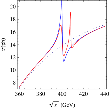
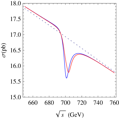
Figure 5: $\sigma(gg\rightarrow t\bar{t})$ for $m_{A}=400$ GeV and $m_{A}=700$ GeV. We include the cases $m_{H}=400,408$ GeV (left) and $m_{H}=700,703$ GeV (right)

is not flat and does not change significantly the angular distribution. Different cuts could be applied to reduce the background for $t\bar{t}$ production at the LHC [7] or even to optimize the contribution from $gg$ versus $q\bar{q}$, but not to enhance the relative effect of the scalars on $\sigma(gg\rightarrow t\bar{t})$.

In Fig. 5 we plot the parton cross section for lower and higher values of the pseudoscalar mass ($m_{A}=400,700$ GeV). We include the cases where the boson $H$ is degenerate with $A$ or slightly heavier ($m_{H}=408$ GeV and $m_{H}=703$ GeV). We see that at lower scalar masses the peak dominates, whereas for large values of $m_{A}$ the dip is the dominant effect. This behaviour, related to the slope of the standard cross section, reduces in both cases the relevance of the mass difference between the scalar and the pseudoscalar Higgses.

4 Little Higgs boson

In LH models the Higgs appears as a pseudo-Goldstone boson of a global symmetry broken spontaneously at the scale $f>v/\sqrt{2}=174$ GeV. The global symmetry introduces an extra $T$ quark that cancels top-quark quadratic corrections to the Higgs mass parameter. The presence of this vectorlike $T$ quark and of a massive scalar singlet (the Higgs of the symmetry broken at $f$) are then generic features in all these models.

Once the electroweak VEV is included the doublet and singlet Higgses (and also the $t$ and $T$ quarks) mix [19, 20]. The singlet component $\approx v/(\sqrt{2}f)$ in $h$ will reduce its coupling both to the top quark and to the gauge bosons and, in turn, $r$ will get a doublet component that couples to these fields.

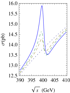
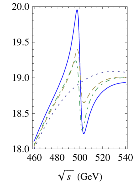
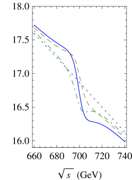
Figure 6: $\sigma(gg\rightarrow t\bar{t})$ for a LH model with $s_{\theta}=0.5$, $m_{r}=500$ GeV and $m_{T}=400,500,700$ GeV. Dashes (dot-dashes) correspond to an amplitude with only the $T$ ($t$) quark loop.

It is easy to see that the most general top-quark Yukawa sector with no quadratic corrections at one loop is

$$-{\cal L}_{t} = \lambda\;\left(f+{r\over\sqrt{2}}\right)\sin{u+h\over\sqrt{2}f}\left(c_{\alpha}t+s_{\alpha}T\right)t^{c}$$ (18)

$$+ \lambda\;\left(f+{r\over\sqrt{2}}\right)\cos{u+h\over\sqrt{2}f}\;TT^{c}+{\rm h.c.}\;,$$

where $u$ and $f$ are VEVs satisfying

$$f\;\sin{u\over\sqrt{2}f}\equiv f\;s_{\theta}={v\over\sqrt{2}}\;.$$ (19)

Eq. (18) becomes

$$-{\cal L}_{t} = \lambda\;\left(f+{r\over\sqrt{2}}\right)\left(s_{\theta}\cos{h\over\sqrt{2}f}+c_{\theta}\sin{h\over\sqrt{2}f}\right)\left(c_{\alpha}t+s_{\alpha}T\right)t^{c}+$$ (20)

$$\lambda\;\left(f+{r\over\sqrt{2}}\right)\left(c_{\theta}\cos{h\over\sqrt{2}f}-s_{\theta}\sin{h\over\sqrt{2}f}\right)TT^{c}+{\rm h.c.}\;.$$

Fermion masses, Yukawa couplings and dimension-5 operators (necessary to check the cancellation of all one-loop quadratic corrections) are then obtained by expanding

$$\cos{h\over\sqrt{2}f}\approx 1-{h^{2}\over 4f^{2}}\;,\;\;\;\sin{h\over\sqrt{2}f}\approx{h\over\sqrt{2}f}$$ (21)

The fermion masses and the Yukawas to the heavier scalar $r$ have the same structure,

$$-{\cal L}_{t}\supset\lambda\;\left(f+{r\over\sqrt{2}}\right)\left(\begin{array}[]{cc}t&T\end{array}\right)\left(\begin{array}[]{cc}s_{\theta}c_{\alpha}&0\\ s_{\theta}s_{\alpha}&c_{\theta}^{2}\end{array}\right)\left(\begin{array}[]{c}t^{c}\\ T^{c}\end{array}\right)\;.$$ (22)

This implies

$$y_{r\bar{t}t}={m_{t}\over f}={\sqrt{2}\;s_{\theta}\;m_{t}\over v}\;\;\;{\rm and}\;\;\;y_{r\bar{T}T}={m_{T}\over f}\;,$$ (23)

where the quarks are mass eigenstates. The mass of the heavier $T$ quark is $m_{T}\approx m_{t}c_{\theta}/(s_{\theta}c_{\alpha})$, and its mixing with the doublet $V_{Tb}\approx s_{\theta}^{2}s_{\alpha}c_{\alpha}/c_{\theta}^{2}$.

The extra Higgs $r$ is somehow similar to the heavier scalar in a doublet plus singlet model, with the doublet component growing with $s_{\theta}=v/(\sqrt{2}f)$. If $s_{\theta}$ is sizeable so is its coupling to the top quark. The coupling to the extra $T$ quark is stronger, but if $r$ is lighter than $2m_{T}$ then its main decay mode will be into $t\bar{t}$. Actually, the doublet component in $r$ may also imply large couplings to the would-be Goldstone bosons for large values of $m_{r}$. More precisely, its decay width $\Gamma_{r}(s)$ at $4m_{t}^{2}<s<4m_{T}^{2}$ is

$$\Gamma_{r}(s)\approx{3\;s_{\theta}^{2}\;s\over 8\pi\;v^{2}}\left[{m_{t}^{2}\;\beta_{t}^{3}\over m_{r}}+{s_{\theta}^{2}\;m_{r}\over 4}\left(\beta_{V}^{3}+{3\over 4}\beta_{V}(1-\beta_{V}^{2})^{2}\right)\;.\right]\;$$ (24)

Therefore, $r$ is a naturally heavy ($m_{r}\approx f$) but narrow scalar resonance with large couplings to quarks and an order one braching ratio to $t\bar{t}$.

In Fig. 6 we plot the parton cross section $\sigma(gg\rightarrow t\bar{t})$ for $s_{\theta}=0.5$, $m_{T}=500$ GeV and several values of $m_{r}$. We separate the contributions from the top and the $T$ quark loops (the second one vanishes at $s=m_{r}^{2}$). The plot is similar to the one obtained for SUSY bosons of the same mass. At higher values of $m_{r}$ the decay width $\Gamma_{r}$ grows, diluting the effect (see Fig.6, right). In contrast, for lower masses the scalar $r$ has a narrow width and is strongly coupled to quarks, which produces a larger effect (in Fig.6, left). The contribution from the standard $t$-quark loop grows with $s_{\theta}$, whereas the contribution from the extra $T$-quark is basically independent of $m_{T}$.

5 Signal at the LHC

Let us now estimate the invariant mass distribution of $t\bar{t}$ events ($m_{t\bar{t}}$) in $pp$ collisions at the LHC. To evaluate the hadronic cross sections we will use the MSTW2008 PDFs [22]. The effect of next-to-leading order (NLO) corrections on the expressions given in previous sections has been studied by several groups (see for example [6, 23]). In particular, the authors in [6] analyze the dependence of ${\rm d}\sigma/{\rm d}m_{t\bar{t}}$ on the choice of renormalization and factorization scales and of PDFs. They show that if the LO cross section is normalized to the NLO one at low values of $m_{t\bar{t}}$, then the deviations introduced by these scales and by the uncertainty in the PDFs at $m_{t\bar{t}}<1$ TeV are small (order 10%). For (scalar and pseudoscalar) Higgs production in $pp$ collisions and Higgs decay, a complete review of NLO results can be found in [1]. From the expressions there we obtain that QCD corrections enhance the production cross section in approximately a 20%, and that the Higgs decay width into $t\bar{t}$ (for $m_{\phi}\gg 2m_{t}$) is also increased in around a 10%. Given these estimates, we have evaluated $pp\rightarrow t\bar{t}$ taking fixed renormalization and factorization scales ($\mu_{R,F}=m_{t}$) and normalizing the LO result to the NLO cross section in [6] with a global factor of 1.3. Our differential cross section coincides then with that NLO result at $m_{t\bar{t}}=500$ GeV.

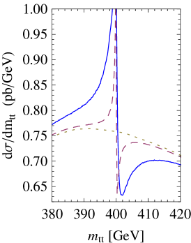
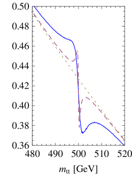
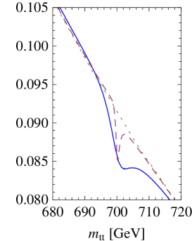
Figure 7: ${\rm d}\sigma/{\rm d}m_{t\bar{t}}$ in SUSY models with $m_{H}=m_{A}=400,500,700$ GeV and $\tan\beta=2$ (solid), $5$ (dashes).

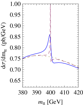
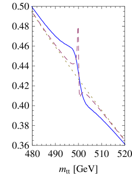
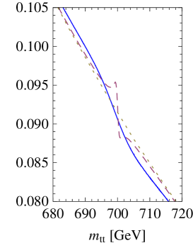
Figure 8: ${\rm d}\sigma/{\rm d}m_{t\bar{t}}$ in LH models with $m_{r}=400,500,700$ GeV and $s_{\theta}=0.5$ (solid), $0.2$ (dashes).

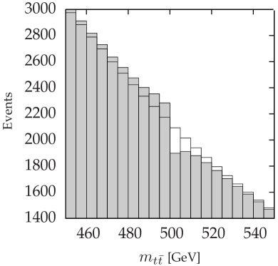
Figure 9: Number of $t\bar{t}$ events in $pp$ collisions at 7 TeV and 1 fb^-1 for $m_{A}=m_{H}=500$ GeV and $\tan\beta=2$ distributed in 5 GeV bins.

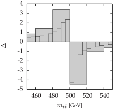
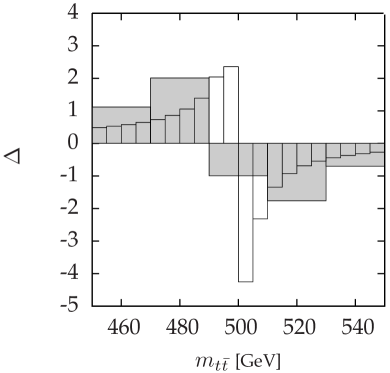
Figure 10: Deviation $\Delta=(N-N_{SM})/\sqrt{N_{SM}}$ in the number of events respect to the standard prediction for two different binning ($m_{A}=m_{H}=500$ GeV and $\tan\beta=2$).

We will take a center of mass energy of 7 TeV. We obtain that at these energies the cross section $pp\rightarrow t\bar{t}$ is dominated by $gg$ fusion, with $q\bar{q}\rightarrow t\bar{t}$ accounting for just 12% of the top-quark pairs. In Figs. 7,8 we plot ${\rm d}\sigma/{\rm d}m_{t\bar{t}}$ for some of the SUSY and LH models described in Sections 3-4. These figures translate the parton-level cross sections in Figs. 3–6 into anomalies in the invariant mass distribution in $pp$ collisions.

To estimate the possible relevance at the LHC of these cross sections, we will calculate the number of $t\bar{t}$ events assuming an integrated luminosity of 1 fb^-1 (expected at the 7 TeV phase of the collider), and we will not apply any cuts. In Fig. 9 we plot the number of events per 5 GeV bin of $m_{t\bar{t}}$ in the SUSY model with $m_{A}=m_{H}=500$ GeV and $\tan\beta=2$. We observe a 5% excess followed by a 9% deficit, with smaller deviations as $m_{t\bar{t}}$ separates from the mass of the extra Higgs bosons. In Fig. 10 we distribute the events in 20 GeV bins and plot the statistical significance

$$\Delta\equiv{N-N_{SM}\over\sqrt{N_{SM}}}$$ (25)

of the deviations, where $N$ is the total number of events in the bin. The typical signal is an increasing excess in a couple of 20 GeV bins that may reach a $+3.4\sigma$ deviation followed by a deficit of $-4.5\sigma$. We find that changing the binning is important in order to optimize the effect. If the same 20 GeV bin includes the peak and the dip (Fig. 10, right) then the maximum deviation is just a $\pm 2\sigma$ effect.

The result is very similar for a LH scalar of $m_{r}=500$ GeV with $s_{\theta}=0.5$. In this LH model we obtain deviations in consecutive 20 GeV bins reaching $+2.5\sigma$ and $-2\sigma$. However, the effect is a bit more localized, and the cancellation if peak and dip coincide in a bin is stronger: it may result in three bins with just $+1.3\sigma$, $+0.6\sigma$ and $-1.2\sigma$ deviations.

The binning is less important for larger Higgs masses. For example, in the SUSY case with $m_{A}=m_{H}=700$ GeV the typical sequence is a couple of 20 GeV bins with a slight $+0.2\sigma$ excess followed by $-1.2\sigma$, $-0.4\sigma$ and $-0.2\sigma$ deficits. In the LH model with $m_{r}=700$ GeV the initial excess (caused by the $T$-quark loop) is a bit more significant, a typical sequence would consist of two bins with $+0.4\sigma$ excess followed by $-0.8\sigma$ and $-0.4\sigma$ deficits.

Let us finally focus on lighter Higgses, as they provide the most promising signal. In Fig. 11 we plot the event distribution (left) and the statistical significance (right) for $\tan\beta=2$ and $m_{A}=m_{H}=400$ GeV, whereas Fig. 12 corresponds to a mass difference of 8 GeV ($m_{A}=400$ GeV and $m_{H}=408$ GeV). The sequence of deviations in both cases would be seen as a clear anomaly, reaching an excess of up to $13\sigma$ (for $m_{H}-m_{A}=-2$ GeV) in a 20 GeV bin. The LH case is analogous but, again, more localized. We obtain an excess of $+3.4\sigma$ in a 20 GeV bin followed by a $-1.7\sigma$ deficit.

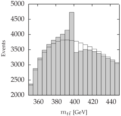
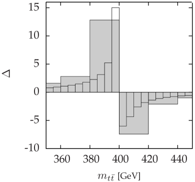
Figure 11: Number of $t\bar{t}$ events in $pp$ collisions (left) and deviation $\Delta$ (right) for $m_{A}=m_{H}=400$ GeV and $\tan\beta=2$.

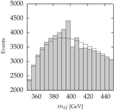
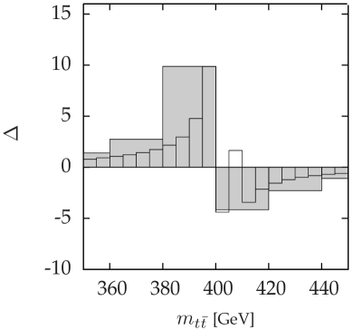
Figure 12: Number of $t\bar{t}$ events in $pp$ collisions (left) and deviation $\Delta$ (right) for $m_{A}=400$ GeV, $m_{H}=408$ GeV and $\tan\beta=2$.

6 Summary and discussion

In models with an extended Higgs sector the extra bosons tend to have large couplings with the top quark that imply a sizeable one-loop production rate at hadron colliders. If the mass of these bosons is not EW but comes from a new scale (e.g., the SUSY or the global symmetry-breaking scales), then they may decay predominantly into $t\bar{t}$. We have studied their effect on the $t\bar{t}$ invariant mass distribution at 7 TeV and 1 fb^-1. We have considered the deviations due to the neutral bosons $A$ and $H$ of the MSSM, and to the scalar $r$ associated to the scale $f$ in LH models. In all cases the interference dominates, invalidating the narrow-width approximation.

The effect for masses around 500 GeV is a peak followed by a dip of similar size. In the SUSY case, values of $m_{H}-m_{A}$ smaller than 3 GeV enhance the deviation, whereas for larger values the effects at $m_{A}<m_{t\bar{t}}<m_{H}$ tend to cancell each other. For $\tan\beta=2$ the significance of the signal, that can be optimized by changing the binning, results in sequences of 20 GeV bins with $+1.4\sigma$, $+3.4\sigma$, $-4.5\sigma$, $-1.0\sigma$ deviations. In LH models the field $r$ couples both to the top and to an extra $T$ quark. The main difference with the SUSY case is that the $T$ quark is heavy and the one-loop form factor to produce the scalar does not get an imaginary part. To have a significant effect the doublet component $s_{\theta}=v/(\sqrt{2}f)$ in $r$ must be large and the extra $T$ quark heavier than $m_{r}/2$ (to close the $T\bar{T}$ decay channel). As $s_{\theta}$ grows $r$ resembles the standard model Higgs, but with a singlet component that reduces its width. The signal at the LHC for $s_{\theta}=0.5$ and $m_{r}=500$ GeV is similar to the SUSY case just described.

At larger scalar masses the peak decreases and the effect is basically a dip in the invariant mass distribution. For $m_{A}=700$ GeV and $\tan\beta=2$ we get a couple of 20 GeV bins with a deficit of $-1.2\sigma$, and $-0.4\sigma$. The effect that one may expect in LH models is alike, although (due to the contribution of the $T$-quark loop) the difference between peak and dip is smaller.

Lower scalar masses provide the most promising scenario. Here the peak dominates both in SUSY and LH models. In the SUSY case with $m_{A}=400$ GeV and $m_{H}=408$ GeV the sequence of 20 GeV bins at 7 TeV and 1 pb^-1 consists of $+2.7\sigma$, $+9.9\sigma$, $-4.2\sigma$ and $-2.3\sigma$ deviations. The signal increases in up to a 30% if the mass difference is smaller (the optimal case is $m_{H}-m_{A}=-2$ GeV). In the LH case with $s_{\theta}=0.5$ and $m_{r}=400$ GeV the sequence reaches a $+3.4\sigma$ deviation. All the effects grow for lower values of $\tan\beta$ and of the LH scale $f$. Obviously, their observability will be better if the LHC reaches 14 TeV and higher luminosities.

An important observation is that the angular distribution of the $t$ quark is unaffected by the intermediate scalar or pseudoscalar bosons. The excess or the deficit caused by its interference with the standard amplitude does not have a flat distribution in the center of mass frame, as one obtains in the narrow-width approximation.

Finally, we would like to comment on the possibility to observe this type of signal at the Tevatron, which may achieve 10 fb^-1 at $\sqrt{s}=1.96$ TeV. The main difference with the LHC is that at the Tevatron 90% of the top-quark pairs are produced through $q\bar{q}$ interactions. Since the signal that we have explored is caused by interference in the $gg\rightarrow t\bar{t}$ channel, for the same integrated luminosity the deviations there would be 9 times weaker than at the LHC (where gluon fusion provides 90% of the top pairs). We find, however, that 1$\sigma$ deviations could be obtained at the Tevatron for low masses of the heavy Higgs bosons. This signal could be enhanced by separating the $t\bar{t}$ events in two or three sets according to the $\cos\theta$ of the final $t$ quark. As we see in Fig. 4, the $gg$ and $q\bar{q}$ contributions at $m_{t\bar{t}}\approx m_{\phi}\approx 500$ GeV have different angular distributions (this difference, however, vanishes at lower invariant masses). One could separate, for example, the events with $\left|\cos\theta\right|$ larger or smaller than 0.6. Then the anomalies in $d\sigma/dm_{t\bar{t}}$ that we have discussed should increase in the $\left|\cos\theta\right|>0.6$ interval.

Although the generic effect on the $t\bar{t}$ invariant mass distribution caused by a scalar field with strong couplings to the top quark is known, we think that it is also important to study particular models. We find that the peculiar anomalies that appear in these two extensions of the standard model may be optimized by changing the binning and by applying the same cuts that select $t\bar{t}$ production from gluon fusion.

References

- [1] A. Djouadi, Phys. Rept. 459 (2008) 1 [arXiv:hep-ph/0503173].
- [2] M. Schmaltz and D. Tucker-Smith, Ann. Rev. Nucl. Part. Sci. 55 (2005) 229.
- [3] M. Perelstein, Prog. Part. Nucl. Phys. 58 (2007) 247.
- [4] K. J. F. Gaemers and F. Hoogeveen, Phys. Lett. B 146 (1984) 347.
- [5] D. Dicus, A. Stange and S. Willenbrock, Phys. Lett. B 333 (1994) 126 [arXiv:hep-ph/9404359].
- [6] R. Frederix and F. Maltoni, JHEP 0901 (2009) 047 [arXiv:0712.2355 [hep-ph]].
- [7] V. Barger, T. Han and D. G. E. Walker, Phys. Rev. Lett. 100 (2008) 031801 [arXiv:hep-ph/0612016].
- [8] T. Aaltonen et al. [CDF Collaboration], Phys. Rev. D 77 (2008) 051102 [arXiv:0710.5335 [hep-ex]].
- [9] V. M. Abazov et al. [D0 Collaboration], Phys. Lett. B 668 (2008) 98 [arXiv:0804.3664 [hep-ex]].
- [10] S. Cabrera [ATLAS Collaboration], J. Phys. Conf. Ser. 171 (2009) 012085.
- [11] U. Baur and L. H. Orr, Phys. Rev. D 76 (2007) 094012 [arXiv:0707.2066 [hep-ph]].
- [12] Z. Hioki and K. Ohkuma, Eur. Phys. J. C 65 (2010) 127 [arXiv:0910.3049 [Unknown]].
- [13] K. Kumar, T. M. P. Tait and R. Vega-Morales, JHEP 0905 (2009) 022 [arXiv:0901.3808 [hep-ph]].
- [14] D. Berdine, N. Kauer and D. Rainwater, Phys. Rev. Lett. 99 (2007) 111601 [arXiv:hep-ph/0703058].
- [15] H. M. Georgi, S. L. Glashow, M. E. Machacek and D. V. Nanopoulos, Phys. Rev. Lett. 40 (1978) 692.
- [16] B. L. Combridge, Nucl. Phys. B 151 (1979) 429.
- [17] R. K. Ellis and J. C. Sexton, Nucl. Phys. B 282 (1987) 642.
- [18] W. de Boer, R. Ehret and D. I. Kazakov, Z. Phys. C 67 (1995) 647 [arXiv:hep-ph/9405342].
- [19] R. Barcelo and M. Masip, Phys. Rev. D 78 (2008) 095012 [arXiv:0809.3124 [hep-ph]].
- [20] R. Barcelo, M. Masip and M. Moreno-Torres, Nucl. Phys. B 782 (2007) 159 [arXiv:hep-ph/0701040].
- [21] J. A. Aguilar-Saavedra, Phys. Rev. D 67 (2003) 035003 [Erratum-ibid. D 69 (2004) 099901].
- [22] A. D. Martin, W. J. Stirling, R. S. Thorne and G. Watt, Eur. Phys. J. C 63 (2009) 189 [arXiv:0901.0002 [hep-ph]].
- [23] S. Frixione, P. Nason and B. R. Webber, JHEP 0308 (2003) 007 [arXiv:hep-ph/0305252].