The Molecular Interstellar Medium of the Local Group Dwarf NGC 6822

Do molecular clouds collapse to form stars at the same rate in all environments? In large spiral galaxies, the rate of transformation of H₂ into stars (hereafter SFE) varies little. However, the SFE in distant objects ($z\sim 1$) is much higher than in the large spiral disks that dominate the local universe. Some small local group galaxies share at least some of the characteristics of intermediate-redshift objects, such as size or color. Recent work has suggested that the Star Formation Efficiency (SFE, defined as the SFRate per unit H₂) in local Dwarf galaxies may be as high as in the distant objects. A fundamental difficulty in these studies is the independent measure of the H₂ mass in metal-deficient environments. At 490 kpc, NGC 6822 is an excellent choice for this study; it has been mapped in the CO(2–1) line using the multibeam receiver HERA on the 30 meter IRAM telescope, yielding the largest sample of giant molecular clouds (GMCs) in this galaxy. Despite the much lower metallicity, we find no clear difference in the properties of the GMCs in NGC 6822 and those in the Milky Way except lower CO luminosities for a given mass. Several independent methods indicate that the total H₂ mass in NGC 6822 is about $5\times 10^{6}$ M_☉ in the area we mapped and less than 10⁷ M_☉ in the whole galaxy. This corresponds to a $N({\rm H}_{2})/I_{\rm CO}\approx 4\times 10^{21}\,{\rm cm^{-2}/(K{\rm\ km\ s^{-1}})}$ over large scales, such as would be observed in distant objects, and half that in individual GMCs. No evidence was found for H₂ without CO emission. Our simulations of the radiative transfer in clouds are entirely compatible with these $N({\rm H}_{2})/I_{\rm CO}$ values. The SFE implied is a factor 5 – 10 higher than what is observed in large local universe spirals. The CO observations presented here also provide a high-resolution datacube (1500 a.u. for the assumed 100 pc distance, $0.41{\rm\ km\ s^{-1}}$ velocity resolution) of a local molecular cloud along the line of sight.

1 Introduction

In the study of star formation in a cosmological or extragalactic context, rather than the details of the collapse of a cloud core to a star, we are interested in understanding why stars form where they do, whether the efficiency varies, and what factors influence the initial mass function (IMF) of the stars. Over the last decade, it has become very clear that the star formation rate per co-moving volume was much higher in the past, some 10 or 20 times the current rate at a redshift of $z\sim 0.5-1$ (e.g. Madau et al. 1996; Heavens et al. 2004; Wilkins et al. 2008). In turn, this shows that the transformation rate of gas into stars was considerably (factor few at least) higher when the universe was roughly half its current age. Galaxies at that time were smaller and of lower metallicity, such that naively at least one would expect that the molecular-to-atomic gas mass ratio would be lower than today (Young & Knezek 1989; Casoli et al. 1998), making the higher efficiency even more surprising. Since stars form from H₂, and not directly from H I (with the possible exception of the so-called Pop. III, or first generation stars), this suggests that either large amounts of molecular hydrogen were available or that for some reason the efficiency of star formation (SFE, defined as the SFR per unit H₂) was particularly high back then. In fact, the SFRs proposed are so much higher than the SFR today that both possibilities may be required. Because at least 10% of the baryons in galaxies today are thought to be in neutral gas (and more than 10% in many cases), an SFR a factor 15 – 20 higher must result at least partially from a higher SFE. If the SFE is higher, then something about the process of star formation is different and there could be other important differences like a change in IMF. Moderate to high redshift galaxies are typically smaller and more gas-rich than today’s spirals and most likely have a slightly subsolar metallicity. They thus resemble today’s small spirals such as M33, or the even smaller NGC 6822, and could be expected to have a low H₂/H I mass ratio. If so, this would make the SFE in these objects even more extreme.

The first step is to learn more about the molecular gas content of galaxies with these properties. Significant quantities of molecular gas were detected far out in the outer disks of NGC 4414 and NGC 6946 (Braine & Herpin 2004; Braine et al. 2007). The outskirts of spirals share the subsolar metallicities and low mass surface densities of small and/or medium/high redshift spirals but not the level of star formation. We are fortunate to have a number of small galaxies in the Local Group close enough that individual giant molecular clouds (GMCs) can be resolved and without distance ambiguities. A first step has been taken, showing that molecular gas forms very far out in M 33 despite the low metallicity and very low ambient pressure (Gardan et al. 2007). NGC 6822 is among the nearest galaxies and is a small late-type dwarf spiral at a distance of about 490 kpc (Mateo 1998) and has a mass and luminosity of roughly 1% of that of our galaxy, thus representing a step down in mass, luminosity and metallicity (roughly $12+log(O/H)\sim 8.1$ (Lee et al. 2006)) with respect to M33, itself a step down in the same quantities from the Milky Way or M31. At 490 kpc, $1\arcsec$ corresponds to 2.4 pc, such that Giant Molecular Clouds (GMCs) can be resolved with large single-dish radiotelescopes.

Observations of the universe at redshifts $z\ga 1$ show that todays large spirals were not present or rare at these earlier epochs. Rather, the galaxies were smaller and had higher star formation rates. They probably had somewhat lower metallicities and were bluer. M33 was found to have a high SFE (Gardan et al. 2007), compared to local universe spirals and IC10 appears to show a high SFE as well (Leroy et al. 2006). NGC 6822 is closer and its molecular gas content has not been mapped systematically until now. Giant Molecular Clouds have been resolved and their physical properties studied in Local Group galaxies both with single dish telescopes (M33 by Gardan et al. 2007; SMC by Rubio et al. 1993; LMC by Fukui et al. 2008; SMC and LMC by Israel et al. 2003b) and with interferometers (M33 by Engargiola et al. 2003; IC 10 by Leroy et al. 2006; M31 by Rosolowsky 2007). NGC 6822 has been observed at many wavelengths to study the interstellar medium (ISM), the dynamics, and trace the star formation. Spitzer FIR observations were carried out recently by Cannon et al. (2006). The atomic gas has been mapped (de Blok & Walter 2000, 2003, 2006a, 2006b; Weldrake et al. 2003) and the molecular gas observed at specific positions with the 15m SEST and JCMT telescope (Israel et al. 1996; Israel 1997a; Israel et al. 2003a).With the OVRO interferometer (Wilson 1994) observed 3 GMCs in NGC 6822 in the Hub V region. Since one of the main questions is whether significant quantities of molecular gas could be present without detectable CO emission, high sensitivity high resolution mapping of large regions allowing the detections of individual possibly optically thick clouds is required. The molecular gas content derived via CO can then be compared with other means of tracing the molecular and atomic gas.

In this article we present the observations and data reduction, mostly of CO (but also $\@element[13]{\mathrm{C}}$O and HCN(1–0) in Hubble V), followed by the production of a catalog of molecular clouds and their properties which we compare with Galactic GMCs. Two methods were used to compile the catalog of cloud sizes, CO intensities, and virial masses: visual inspection of the data cube and the CPROPS algorithm (Rosolowsky & Leroy 2006). A map of the total CO emission is then compared (Sect. 6) with other means of estimating the H₂ column density, leading to a discussion of the SFE in NGC 6822. We then present several models using the CLOUDY (Ferland et al. 1998) code to compare several spectral synthesis models with the observations presented in the preceding sections. Finally, two regions of NGC 6822 are discussed in more detail – Hubble V and X. A local molecular cloud is present along the line of sight to NGC 6822 and has thus been observed serendipitously at high spectral and spatial resolution. These data are presented in the last section.

Figure 1: Main image GALEX FUV filter image of NGC 6822. The yellow box indicates the area observed in CO. The dashed, dotted, and solid yellow contours indicate the H I column density at $12\arcsec\times\ 42\arcsec$ resolution from de Blok & Walter (2006b) at column densities of 0.5, 1, and 1.5 $\times\ 10^{21}$ cm^-2 respectively. The white cross corresponds to (0,0) offsets of the HERA CO(2-1) map. Bottom right HI contour at a column density of $0.5\times 10^{21}$ cm^-2. The dashed rectangle corresponds to the GALEX FUV map above, the solid line contour to the area observed in CO.

Table 1: Parameters for NGC 6822.

$\alpha_{o}$(J2000)a	$19^{\mathrm{h}}44^{\mathrm{m}}57\ \aas@@fstack{s}83$
$\delta_{o}$(J2000)a	$-14\degr 48\arcmin 11\arcsec$
Distanceb	$490\pm 40$ kpc
$V_{\mathrm{LSR}}$	$-47$ ${\rm\ km\ s^{-1}}$
Metallicityc	$\simeq 0.3\leavevmode\nobreak\ \mathrm{Z}_{\sun}$
Total optical luminosityb	$\sim 9.4\times 10^{7}\leavevmode\nobreak\ \mathrm{L}_{\sun}$
Total H I massd	$1.34\times 10^{8}\leavevmode\nobreak\ \mathrm{M}_{\sun}$
Dynamical masse	$3.2\times 10^{9}\leavevmode\nobreak\ \mathrm{M}_{\sun}$

• (0,0) offset of our HERA CO(2-1) map

• Mateo (1998)

• Skillman et al. (1989); Lee et al. (2006)

• de Blok & Walter (2006b)

• de Blok & Walter (2006b); Weldrake et al. (2003)

2 Observations

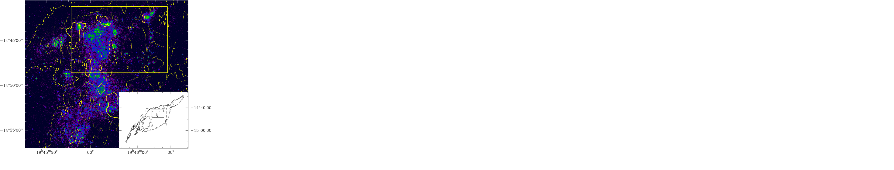
NGC 6822 was observed during three separate runs at the IRAM 30 meter telescope in November 2006, February/March 2007 and August 2008 in mostly good weather. All mapping was done using the HERA array of 9 dual polarization receivers (Schuster et al. 2004) in the CO(2–1) line, whose rest frequency is 230.53799 GHz which gives a nominal resolution of $11.4\arcsec$ for this line. The On-The-Fly mode was used to cover a roughly $11\times 7$ arcminute region, scanning along the RA and then Dec directions and observing a reference position offset from our central position by $(100\arcsec,500\arcsec)$ before and after each scan. The reference position was chosen to be outside of the $5\times 10^{20}$ cm^-2 contour of the H I column density map (see Fig. 1).

The VESPA backend was used with a channel spacing of 312 kHz or $0.406{\rm\ km\ s^{-1}}$ covering velocities from $+20\mbox{ to }{-150{\rm\ km\ s^{-1}}}$, well beyond the rotation curve of NGC 6822. Local (Galactic) emission was detected around ${+5{\rm\ km\ s^{-1}}}$ (see Sect. 10). All data are presented in the main beam temperature scale and we have assumed forward and main beam efficiencies of $\eta_{for}=0.90$ and $\eta_{mb}=0.52$ for the HERA observations, the sensitivity is then ${\rm 9.6Jy/K}$ (Schuster et al. 2004).

Also during the November 2006 run, during poorer weather than for the more demanding HERA observations, the major H II region Hubble V was observed in the $\@element[13]{\mathrm{C}}$O(1–0), $\@element[13]{\mathrm{C}}$O(2–1), HCN(1–0), and $\@element[12]{\mathrm{C}}$O(1–0) lines. Wobbler switching was used with a throw of $60\arcsec$ and the 100 kHz and VESPA backends were used, yielding spectral resolutions of respectively 0.27, 0.43, 1.06, and 0.26 ${\rm\ km\ s^{-1}}$ for the lines above. The forward and main beam efficiencies at these frequencies are assumed to be respectively $\eta_{for}=0.95,\ 0.91,\ 0.95,\ 0.95$ and $\eta_{mb}=0.75,\ 0.55,\ 0.78,\ 0.74$. The data reduction of the HERA observations is described in the next section. For the Hubble V data, bad channels were eliminated and spectra were averaged, yielding the spectra discused in Sect. 9.2.

3 Reduction of HERA data

The On-The-Fly mapping technique with a multi-beam array generates a huge amount of spectra, more than a million in the case of NGC 6822. Inspection of individual spectra is thus not possible and the reduction was automated. All data reduction was done within the Gildas CLASS and GREG software packages. After filtering out the spectra taken in very poor conditions (T${}_{sys}>1500$ K), we treated the main problem which was the slight platforming where the sub-bands of the auto-correlator backend were stitched together. The platforming effect is the result of different non-linearities in the sampling stages of the subbands. In case of changing total power levels as compared to the reference position this introduces offsets in the subbands. The steps were very small in our case but sufficient to affect weak lines. For each spectrum, the average value for each subband, outside of the line windows as far as possible, was subtracted from each channel of the sub-band, eliminating the platforming. This process takes out a zero-order baseline.

There is a known baseline ripple with HERA (Schuster et al. 2004) corresponding to a reflection off the secondary mirror at 6.9 MHz or 9 km s^-1. Since the pixels (receivers) are affected at quite different levels and because the width of the ripple is close to that of molecular clouds, we tested each spectrum and when the ripple was strong enough to be identified in the individual (i.e. roughly 1sec integration time) spectra, the corresponding Fourier frequency was replaced by an interpolation based on adjacent frequencies. This fairly standard filtering is often applied “blindly” to all spectra but we only applied it when necessary.

In order to create the datacube, we created a data table with the TABLE command within CLASS90 and then used the XY_MAP task in GREG with parameters such that the final resolution became $15\arcsec$, or about 36 pc at the distance of NGC 6822. Data cubes with different resolutions where always generated directly from the original data by convolution with the corresponding kernel size.

4 The individual molecular clouds in NGC 6822

4.1 Identification by visual inspection

The final beam width of the CO observations is about 30 pc and because of the beam dilution we do not expect to see clouds with sizes under 10 pc. We define clouds as structures similar to Galactic Giant Molecular Clouds (GMCs) that appear as gravitationally bound and non transient structures a few ten of parsecs in size. Figure 2 shows the CO(2–1) and H I spectra of the clouds found in the original $15\arcsec$ datacube, showing both the CO and H I intensity scales. The spectra are averages over the 50% brightness contour. It is clear that all strong CO lines are close to the H I peak in velocity. However, cloud 13 is at either the edge of the H I line or possibly part of a second H I feature with a brightness of 25 K. Cloud 14 is also near the edge of the H I line although mostly within the 30 K H I brightness temperature level used to define the CO line window in the next section.

Figure 2: Spectra of individual clouds, (black) H I 21cm line, (red) CO(2-1) line, (blue) Gausian line fit to the narrowest component, the physical parameters of these clouds can be found in Table 2.

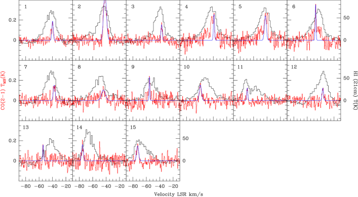
Gaussian fits were made to the individual clouds in order to determine linewidths and central velocities. In several cases, more than one gaussian was required. Since one of the goals is to measure line width and cloud sizes for NGC 6822 clouds and compare to Milky Way clouds, only the stronger (in antenna temperature) and narrower gaussian was used to define the line widths and sizes of the individual clouds. Line areas are computed by summing channels in a velocity range determined manually for each cloud. The line intensities, systemic velocities and widths are averages over the 50% brightness level of each cloud.

Spectra for clouds 4 and 5 show that these clouds are only partially spatially resolved. Contour maps of the integrated intensity for the two components 4 and 5 (Fig. 3) indicate that the emission can be separated into two clouds separated by about 9 arcseconds.

Figure 3: Contour integrated intensity maps of clouds 4 (solid lines) and 5 (dashed lines) contours every $0.1\rm{K}{\rm\ km\ s^{-1}}$. The emission peaks are separated by about 9 arcsec showing that there are clearly two separate clouds.

Table 2 provides positions, velocities, linewidths, and estimated sizes for each cloud. In some cases, clouds were separated by summing over different velocity ranges, enabling cloud separations smaller than the beamsize. On the individual maps, corresponding to each cloud, the 50% brightness level was defined for each cloud, allowing the effective radius (see Sect. 4.2.1) of the cloud to be estimated as $R_{e}=(1.92/2\sqrt{2\ln 2})\sqrt{polygon\ area\arcsec-15\arcsec^{2}}$ and converted to pc. The subtraction of the beam area ($15^{2}$) enables a simple deconvolution with the the beamsize assuming in average a gaussian intensity distribution of the cloud emission, the numerical factor converts the FWHM to an effective radius. Below about 10 pc, the beam dilution makes the detection of individual clouds difficult.

The CO(2–1) integrated intensities (col. 7) are obtained by summing channels within $V=V_{o}\pm\Delta V$. Virial masses (col. 8) are calculated from $M_{vir}=1040R_{e}\left({\Delta V}/{2\sqrt{2\ln 2}}\right)^{2}$ following Solomon et al. (1987) and using their form factor of 2.7. For comparison, cloud masses (including He) can be estimated as $M=I_{\rm CO(2-1)}\times 2500\times({\rm size/20pc})^{2}$M_☉ using a “standard” Milky Way factor of $\ratio=2\times 10^{20}\,{\rm cm^{-2}/(K{\rm\ km\ s^{-1}})}$ (Dickman et al. 1986) and a CO(2–1)/(1–0) line ratio of 0.7 (Sawada et al. 2001). Inspection of the values shows that the Galactic $N({\rm H}_{2})/I_{\rm CO}$ factor yields masses far below the virial masses. This is well known for clouds in low metallicity galaxies (e.g. Rubio et al. 1993; Israel 1997b). The virial masses themselves may be underestimates of the true H₂ masses if the H₂ extends beyond where the CO is detected. The following column provides an independent estimate of the H₂ mass (see Sect. 6.3 for details) and resulting $N({\rm H}_{2})/I_{\rm CO}$ factor.

Table 2: Properties for the clouds identified by eye (Top), and by the CPROPS package (Bottom).

The clouds whose numbers are in bold face correspond to our final sample of clouds

Cloud	$\left.\alpha_{\mathrm{off}}\right.^{\mathrm{a}}$	$\left.\delta_{\mathrm{off}}\right.^{\mathrm{a}}$	$\mathrm{V}_{\mathrm{LSR}}$	FWHM	${\rm R_{e}}$	$\mathrm{I}_{\mathrm{CO}}$	$\left.\mathrm{M}_{\mathrm{vir}}\right.^{\mathrm{b}}$	$\left.\mathrm{M}_{\mathrm{H_{2}}}\right.^{\mathrm{c}}$	$\left.N(\mathrm{H_{2}})/\mathrm{I}_{\mathrm{CO}}\right.^{\mathrm{d}}$
	arsec	arcsec	${\rm\ km\ s^{-1}}$	${\rm\ km\ s^{-1}}$	pc	$\mathrm{K}{\rm\ km\ s^{-1}}$	$\mathrm{M}_{\sun}$	$\mathrm{M}_{\sun}$	$\frac{\mathrm{cm}^{-2}}{\mathrm{K}{\rm\ km\ s^{-1}}}$
GMC NGC6822 1	$-48$	330	$-43.2$	$1.5\pm 0.9$	$22_{-14}^{+9}$	$0.92_{-0.10}^{+0.10}$	$9.3_{-8.7}^{+24}\times 10^{3}$	$3.6_{-0.8}^{+1.4}\times 10^{4}$	$1.4_{-0.2}^{+0.2}\times 10^{21}$
GMC NGC6822 $2^{\mathrm{e}}$	$-68.5$	299	$-42.4$	$5.1\pm 0.4$	$29_{-6}^{+5}$	$2.47_{-0.13}^{+0.14}$	$1.9_{-0.5}^{+0.5}\times 10^{5}$	$3.1_{-0.6}^{+0.3}\times 10^{4}$	$3.0_{-0.3}^{+0.3}\times 10^{20}$
GMC NGC6822 3	80	58	$-38.0$	$2.4\pm 0.5$	$38_{-21}^{+15}$	$0.36_{-0.06}^{+0.07}$	$4.1_{-3}^{+4.2}\times 10^{4}$	$9.5_{-3.7}^{+3.5}\times 10^{4}$	$4.3_{-1.1}^{+1.6}\times 10^{21}$
GMC NGC6822 4	39	25	$-39.9$	$2.0\pm 0.6$	$18_{-10}^{+6}$	$1.34_{-0.09}^{+0.10}$	$1.2_{-0.3}^{+0.1}\times 10^{5}$	$1.2_{-0.3}^{+0.1}\times 10^{5}$	$3.1_{-0.3}^{+0.4}\times 10^{21}$
GMC NGC6822 5	35	24	$-43.2$	$3.4\pm 1.1$	$19_{-9}^{+8}$	$1.52_{-0.13}^{+0.11}$	$4.1_{-0.3}^{+0.6}\times 10^{4}$	$1.2_{-0.3}^{+0.2}\times 10^{5}$	$2.5_{-0.2}^{+0.5}\times 10^{21}$
GMC NGC6822 6	30	16	$-48.3$	$1.6\pm 0.4$	$12_{\textrm{ \ldots}}^{+15}$	$0.82_{-0.07}^{+0.05}$	$5.8_{\textrm{ \ldots}}^{+14}\times 10^{3}$	$4.7_{-1.4}^{+1.4}\times 10^{4}$	$2.4_{-0.2}^{+0.3}\times 10^{21}$
GMC NGC6822 7	$-10$	364	$-38.1$	$3.2\pm 0.4$	$27_{-15}^{+11}$	$0.48_{-0.07}^{+0.06}$	$5.2_{-3.4}^{+4.1}\times 10^{4}$	$4.9_{-1.0}^{+0.2}\times 10^{3}$	$2.8_{-1.2}^{+1.6}\times 10^{20}$
GMC NGC6822 8	31	61	$-44.8$	$2.4\pm 1.4$	$14_{\textrm{ \ldots}}^{+28}$	$0.58_{-0.14}^{+0.13}$	$1.5_{\textrm{ \ldots}}^{+9.9}\times 10^{4}$	$4.1_{-2.5}^{+5.1}\times 10^{4}$	$2.8_{-0.5}^{+1.0}\times 10^{21}$
GMC NGC6822 9	7	54	$-56.0$	$1.4\pm 0.4$	$\textrm{ \ldots}_{\textrm{ \ldots}}^{+13}$	$0.57_{-0.10}^{+0.04}$	$\textrm{ \ldots}_{\textrm{ \ldots}}^{+7.9}\times 10^{3}$	$7.6_{-1.6}^{+4.2}\times 10^{3}$	$8.2_{-0.7}^{+1.7}\times 10^{20}$
GMC NGC6822 10	0	26	$-60.1$	$3.9\pm 1.0$	$33_{-17}^{+17}$	$0.59_{-0.10}^{+0.07}$	$9.4_{-6.9}^{+13}\times 10^{4}$	$7.6_{-2.9}^{+3.4}\times 10^{4}$	$2.6_{-0.7}^{+1.0}\times 10^{21}$
GMC NGC6822 11	$-358$	208	$-70.3$	$2.0\pm 0.9$	$28_{\textrm{ \ldots}}^{43}$	$0.23_{-0.07}^{+0.07}$	$2.1_{\textrm{ \ldots}}^{+9.1}\times 10^{4}$	$\textrm{ \ldots}_{\textrm{ \ldots}}^{\textrm{ \ldots}}\,{}^{\mathrm{h}}$	$\textrm{ \ldots}_{\textrm{ \ldots}}^{\textrm{ \ldots}}\,{}^{\mathrm{h}}$
GMC NGC6822 12	$55$	$287$	$-37.6$	$2.6\pm 0.5$	$23_{\textrm{ \ldots}}^{+28}$	$0.23_{-0.02}^{+0.06}$	$2.9_{\textrm{ \ldots}}^{+6.3}\times 10^{4}$	$\textrm{ \ldots}_{\textrm{ \ldots}}^{+3.0}\times 10^{3}$	$\textrm{ \ldots}_{\textrm{ \ldots}}^{+1.7}\times 10^{20}$
GMC NGC6822 13	$49$	$364$	$-54.7$	$1.7\pm 0.4$	$\textrm{ \ldots}_{\textrm{ \ldots}}^{+34}$	$0.26_{-0.07}^{+0.05}$	$\textrm{ \ldots}_{\textrm{ \ldots}}^{+2.7}\times 10^{4}$	$\textrm{ \ldots}_{\textrm{ \ldots}}^{\textrm{ \ldots}}\,{}^{\mathrm{h}}$	$\textrm{ \ldots}_{\textrm{ \ldots}}^{\textrm{ \ldots}}\,{}^{\mathrm{h}}$
GMC NGC6822 14	$-331$	$372$	$-76.0$	$3.0\pm 1.0$	$\textrm{ \ldots}_{\textrm{ \ldots}}^{+15}$	$0.32_{-0.08}^{+0.08}$	$\textrm{ \ldots}_{\textrm{ \ldots}}^{+4.5}\times 10^{4}$	$\textrm{ \ldots}_{\textrm{ \ldots}}^{\textrm{ \ldots}}\,{}^{\mathrm{h}}$	$\textrm{ \ldots}_{\textrm{ \ldots}}^{\textrm{ \ldots}}\,{}^{\mathrm{h}}$
GMC NGC6822 15	$-386$	$57$	$-73.8$	$3.6\pm 0.8$	$24_{-16}^{+21}$	$0.53_{-0.12}^{+0.06}$	$5.8_{-4.7}^{+11}\times 10^{4}$	$5.5_{-1.4}^{+1.3}\times 10^{4}$	$2.9_{-01.2}^{+1.7}\times 10^{21}$

Cloud	$\left.\alpha_{\mathrm{off}}\right.^{\mathrm{a}}$	$\left.\delta_{\mathrm{off}}\right.^{\mathrm{a}}$	$\mathrm{V}_{\mathrm{LSR}}$	FWHM	${\rm R_{e}}$	${\rm R_{ex}}$	$\mathrm{I}_{\mathrm{CO}}$	$\left.{\mathrm{M}_{\mathrm{vir}}}\right.^{\mathrm{b}}$	$\left.\mathrm{M}_{\mathrm{H_{2}}}\right.^{\mathrm{c}}$	$\left.N(\mathrm{H_{2}})/\mathrm{I}_{\mathrm{CO}}\right.^{\mathrm{d}}$
	arsec	arcsec	${\rm\ km\ s^{-1}}$	${\rm\ km\ s^{-1}}$	pc	pc	$\mathrm{K}{\rm\ km\ s^{-1}}$	$\mathrm{M}_{\sun}$	$\mathrm{M}_{\sun}$	$\frac{\mathrm{cm}^{-2}}{\mathrm{K}{\rm\ km\ s^{-1}}}$
GMC NGC6822 1	$-50$	$331$	$-40.2$	$5.5\pm 3.5^{\mathrm{g}}$	$15\pm 14$	$38$	$0.9\pm 0.3$	$8.5\pm 9.2\times 10^{4}\,{}^{\mathrm{g}}$	$5.1\times 10^{4}$	$9.9\times 10^{20}$
GMC NGC6822 2	$-71$	$301$	$-41.3$	$6.2\pm 1.4$	$32\pm 4$	$86$	$1.2\pm 0.1$	$2.3\pm 0.5\times 10^{4}$	$9.8\times 10^{4}$	$4.2\times 10^{20}$
GMC NGC6822 3	$83$	$59$	$-37.0$	$2.2\pm 1.9$	$32\pm 13$	$54$	$0.2\pm 0.1$	$2.8\pm 2.6\times 10^{4}$	$1.1\times 10^{5}$	$6.4\times 10^{21}$
GMC NGC6822 4	$38$	$25$	$-39.2$	$2.1\pm 3.2$	$15\pm 21$	$12$	$1.0\pm 1.3$	$1.3\pm 2.3\times 10^{4}$	$1.2\times 10^{5}$	$4.0\times 10^{21}$
GMC NGC6822 5	$35$	$24$	$-42.6$	$3.9\pm 6.2$	$10\pm 22$	$\ldots^{\mathrm{\,i}}$	$1.4\pm 2.2$	$2.9\pm 7.6\times 10^{4}$	$8.8\times 10^{4}$	$2.8\times 10^{21}$
GMC NGC6822 6	$30$	$17$	$-47.1$	$3.2\pm 3.0$	$15\pm 29$	$33$	$0.7\pm 0.2$	$2.8\pm 6.3\times 10^{4}$	$9.9\times 10^{4}$	$3.0\times 10^{21}$
GMC NGC6822 7	$-17$	$359$	$-38.1$	$2.1\pm 1.8$	$31\pm 17$	$47$	$0.3\pm 0.2$	$2.5\pm 2.4\times 10^{4}$	$\ldots^{\mathrm{h}}$	$\ldots^{\mathrm{h}}$
GMC NGC6822 8	$33$	$62$	$-43.2$	$4.6\pm 6.0$	$19\pm 20$	$37$	$0.3\pm 0.2$	$7.5\pm 14\times 10^{4}$	$9.5\times 10^{4}$	$4.7\times 10^{21}$
GMC NGC6822 9	$7$	$54$	$-55.3$	$2.1\pm 1.8$	$10\pm 31$	$31$	$0.3\pm 0.1$	$0.8\pm 2.3\times 10^{4}$	$3.6\times 10^{4}$	$2.6\times 10^{21}$
GMC NGC6822 10	$0$	$27$	$-59.4$	$4.6\pm 2.7$	$25\pm 7$	$55$	$0.5\pm 0.1$	$9.6\pm 6.1\times 10^{4}$	$1.4\times 10^{5}$	$3.1\times 10^{21}$
GMC NGC6822 11	$-365$	$210$	$-69.4$	$1.7\pm 1.8$	$11\pm 27$	$16$	$0.2\pm 0.2$	$0.6\pm 1.7\times 10^{4}$	$\ldots^{\mathrm{h}}$	$\ldots^{\mathrm{h}}$

• Offsets with respect to the reference position $(\alpha_{o},\delta_{o})=(19^{\mathrm{h}}44^{\mathrm{m}}57\ \aas@@fstack{s}8,-14\degr 48\arcmin 11\arcsec)$

• Virial mass following Solomon et al. (1987) using ${\rm R_{e}}$ and $\Delta V$ (see Sect. 4)

• $\mathrm{H}_{2}$ mass estimate from ${\rm 8\mu m}$ emission (see Sect. 6.3).

• X conversion factor for individual clouds using $N(\mathrm{H_{2}})$ estimated from ${\rm 8\mu m}$ emission (see Sect. 6.3).

• Hubble V (Hubble 1925)

• see Sect. 4

• The CPROPS computed FWHM is clearly overestimated compared to the one computed by hand by a factor of about 3. ${\rm M_{vir}}$ being proportional to ${\rm FWHM^{2}}$, this explains the order of magnitude difference between the computed virial masses for this cloud.

• The computed ${\rm H_{2}}$ mass for these clouds was found to be negative.

• The deconvolved size was not defined.

4.2 Automated cloud identification

4.2.1 CPROPS

We have also used the CPROPS program (Rosolowsky & Leroy 2006) to identify GMCs and measure their physical properties in an unbiased way. CPROPS first assigns the measured emission to clouds by identifying emission above a $4\sigma$ noise level and then decomposing the emission into individual clouds (see Rosolowsky & Leroy 2006, for further details). It then extrapolates physical properties such as cloud sizes and masses to 0K noise level, independent of the beamsize (i.e. deconvolved). Using CPROPS, we find 11 clouds all of which have also been identified as such by eye. The cloud properties as identified by CPROPS are presented in the lower part of Table 2. We were not able to setup CPROPS in such a way that all the eye-identified clouds were found without a large number of clouds we do not believe are real being also identified by CPROPS. CPROPS was used with the following parameters: a constant distance DIST equal to $490$ kpc; the /NONUNIFORM parameter along with a custom noise map computed from velocity channels without any signal (i.e. outside the rotation curve), to take into account non uniform noise over the CO map; the following values for the decomposition parameters FSCALE=2.0, SIGDISCONT=0 to ensure that each area of non-contiguous emission is assigned to an individual independent cloud.

Using the identified cloud emissions, CPROPS computes four initial quantities through an extrapolation to a $0\$K noise level: the $\sigma_{x}$ and $\sigma_{y}$ spatial dispersions, the velocity dispersion $\sigma_{v}$ and the CO flux ${\rm F_{CO}}$. From these quantities, the following physical quantities are deduced. An effective radius $R_{e}$ (col. 6) is obtained using the formula:

$$R_{e} = \eta\sigma_{r}$$ (1)

$$\sigma_{r} = \sqrt{\sqrt{\sigma_{min}^{2}-\left(\frac{FWHM_{beam}}{2\sqrt{2\ln 2}}\right)^{2}}\sqrt{\sigma_{max}^{2}-\left(\frac{FWHM_{beam}}{2\sqrt{2\ln 2}}\right)^{2}}}$$ (2)

Where $\eta=3.4/\sqrt{\pi}=1.92$ is an empirical geometric factor from Solomon et al. (1987) to take into account the radial distribution of the gas density inside the molecular cloud and $\sigma_{min}$ and $\sigma_{max}$ are spatial dispersions along the major and minor axes of the cloud.

For a few of the clouds identified by CPROPS, the minimum dispersion $\sigma_{min}$ was found to be smaller than the beamsize. In these cases we have chosen to use an arbitrary value of $\sigma_{min}$ corresponding to an effective minimum spatial dispersion of $10$pc.

We have also computed an extrapolated radius (col. 7)

$$R_{ex}=\frac{\sqrt{A_{2\sigma}-(FWHM_{beam}/2\sqrt{2\ln 2})^{2}}}{\pi}$$ (3)

where $A_{2\sigma}$ is the area of the individual clouds extrapolated down to a $2\sigma$ level projected on the sky plane (see Rosolowsky & Leroy 2006, for details).

The clouds’ integrated CO(2–1) intensities (col. 8, lower part of Table 2) were obtained for each cloud by dividing the CPROPS computed ${\rm L_{CO}}$ luminosity by the projected area of each individual cloud, $A_{2\sigma}$, at the two sigma level.

4.2.2 Comparing with eye identification

For the subset of clouds which have both been identified by eye and by the CPROPS package, we can compare the physical properties obtained by the two independent methods. Table 2 shows the properties computed by hand for the 15 clouds identified by eye, and by CPROPS for the first eleven which have also been identified with CPROPS. Each property is computed slightly differently for the two methods and the next paragraphs will explain these differences.

In the manual identification method, the offsets for the cloud positions are obtained by taking the average position in right ascension and declination of the pixels inside of the half maximum contour of the cloud emission. In the case of CPROPS, the offsets are equal to the first moments of the cloud emission (down to $2\sigma$) along the right ascension and declination axis. The positions are in general the same to within 0.2 beam fwhm.

The systemic velocity is taken as the average of the gaussian fit to the CO line (see Sect. 4.1) for the manual identification method, in the case of CPROPS it is computed as the first moment along the velocity axis of the cloud emission down to $2\sigma$. Following the same idea, the line width are computed in the manual case as the the function width at half maximum of the fitted gaussian and as the second moment converted to FWHM by multiplying by $2\sqrt{2\ln 2}$ for the properties derived from CPROPS. An effective radius $R_{e}$ is obtained using Eq. 2 and preceding section. In the case of the manual identification, the effective radius was obtained in the following way.

$$R_{e}^{eye}=\frac{1.92}{2\sqrt{2\ln 2}}\sqrt{A_{\frac{1}{2}}-A_{beam}}$$ (4)

where $A_{\frac{1}{2}}$ is the area in ${\rm pc^{2}}$ inside the contour at half of the peak integrated intensity for each cloud. And $A_{beam}=1270pc^{2}$ is the area subtended by the $15\arcsec$ beam at a distance of $490kpc$. The $2\sqrt{2\ln 2}$ factor converts the FWHM to dispersion and the $1.92$ from dispersion to effective radius.

The CO intensity was computed using CPROPS CO luminosity and dividing it by the area $A_{2\sigma}$ of the cloud computed above. In the case of the manual selection, the emission inside the 50% level contour was summed over the velocity range $V_{o}\pm\Delta V$ and multiplied by the $0.41{\rm\ km\ s^{-1}}$ channel width.

In both cases, the virial mass was obtained using the following formula from (Solomon et al. 1987):

$$M_{vir}=1040R_{e}\left(\frac{\Delta V}{2\sqrt{2\ln 2}}\right)^{2}$$ (5)

The uncertainties in the virial mass estimates are dominated by the hypothesis that the molecular clouds are indeed gravitationally bound and by the value of the geometric factor describing the density distribution of the gas. The marginally gravitationally bound case of a cloud in isolation with no magnetic field would yield masses a factor 2 less than virial. The virial masses are widely used because clouds have magnetic fields, are not isolated, and collapse to form stars.

The ${\rm H_{2}}$ masses (col. 9 for top and col. 10 for bottom parts of Table 2) are derived following the method described in Sect. 6.3, using the 50% contour in the case of the manual identification and the $2\sigma$ contour for CPROPS.

The last column in Tab 2, $N({\rm H}_{2})/I_{\rm CO}$ is the ${\rm H_{2}}$ column density derived in Sect. 6.3 divided by ${\rm I_{CO}}$.

4.3 Estimation of errors

For the CPROPS identification method, the uncertainties for the quantities FWHM, ${\rm R_{e}}$, ${\rm I_{CO}}$ and ${\rm M_{vir}}$ are computed using the bootstrapping method of CPROPS (see details in Rosolowsky & Leroy 2006). We now describe the computation of the uncertainties in the case of the identification of clouds by eye. The FWHM line width and associated error are computed with the CLASS software gaussian line fitting algorithm. Then, using the line widths obtained, the unvertainty in integrated intensity $\sigma_{Kkm/s}$ is calculated for each cloud. The uncertainty on the size ${\rm R_{e}}$ is estimated by calculating ${\rm R_{e}}$ from contours (cloud sizes) placed at $I_{peak}/2-\sigma_{Kkm/s}$ and $I_{peak}/2+\sigma_{Kkm/s}$, thus bracketing the cloud size obtained using the $I_{peak}/2$ contour. This gives respectively an upper (lower) bound on the value of ${\rm R_{e}}$. The errors are then propagated into the Virial mass. For each cloud, the contours defined at $I_{peak}/2\pm\sigma_{Kkm/s}$ are used to compute the molecular gas mass (see Sect. 6) from the 8 micron map and thus estimate the uncertainties in the molecular gas mass (Tab. 2 col. 9) and the $N({\rm H}_{2})/I_{\rm CO}$ factor (Tab. 2 col. 10).

5 The size-linewidth relation for the molecular clouds in NGC 6822

Figure 4: Size vs linewidth for molecular clouds in NGC 6822, open and filled circles correspond respectively to measured and deconvolved sizes (see Sect. 4). Filled squares correspond to physical properties computed with the CPROPS package. ${\rm\left.\Delta V\propto{R_{e}}\right.^{0.5}}$ is the galactic relationship from Solomon et al. (1987). Notwithstanding considerable scatter, the distribution of the clouds (corrected for finite beamsize) in this diagram appears consistent with a size-linewidth relation similar to that in the Milky Way.

Figure 5: Virial mass vs CO luminosity for molecular clouds in NGC 6822, open and filled circles correspond respectively to measured and deconvolved sizes (see Sect. 4). Filled squares correspond to physical properties computed with the CPROPS package. The line ${\rm M_{vir}=9796\left(\frac{L_{CO(1-0)}}{1000}\right)^{0.8}}$ is the galactic relationship from Solomon et al. (1987), the dashed line corresponds to a constant galactic $N({\rm H}_{2})/I_{\rm CO}$ ratio of $2\times 10^{20}\,{\rm cm^{-2}/(K{\rm\ km\ s^{-1}})}$. The virial masses are systematically larger for a given luminosity in NGC 6822 compared to clouds in the Milky Way.

Figures 4 and 5 show respectively the size-linewidth relation ($\Delta V$ vs. $R_{e}$) and the virial mass vs CO luminosity, showing in both cases the Galactic values taken from Solomon et al. (1987) as a straight line. The distribution of the clouds in NGC 6822 appears consistent with a size-linewidth relation similar to that in the Milky Way GMCs. In recent work Heyer et al. (2009) obtain lower H₂ masses and a dependency on the square root of the surface density, the variation we obtain in these parameter is much to low to reach a conclusion. Like Solomon et al. (1987), they concluded that GMCs are gravitationally bound.

Fig. 5 shows that there is a factor several difference between the virial masses of the NGC 6822 clouds and the masses obtained from the size and CO(2–1) intensities using a Galactic $N({\rm H}_{2})/I_{\rm CO}$ conversion factor. For a ${\rm{CO(2-1)}/{CO(1-0)}}$ ratio of 0.7, the difference is $5\mbox{ -- }6$, the true $N({\rm H}_{2})/I_{\rm CO}$ value is then at least $5\mbox{ -- }6$ times higher than in the Milky Way. Due to the low metallicity of NGC 6822, cloud sizes as seen in CO are probably underestimated compared to Galactic observations, where the shielding will be much more efficient to protect CO molecules and allow the CO size to be similar to the total size of the H₂ dominated region (the molecular cloud). Because the line width is presumably determined by the total mass, the virial masses should be underestimated linearly with the size. CO luminosities, used when applying a $N({\rm H}_{2})/I_{\rm CO}$ factor, should be underestimated twice as much in proportion because luminosities vary with the square of the size. In the following section we try to estimate the factor by means without these drawbacks.

6 The total molecular mass of NGC 6822

In this section we describe how we make a CO integrated intensity map to trace the H₂ column density. In order to test whether there could be substantial amounts of molecular gas without associated CO emission, we use two other alternative methods (similar to Israel 1997a) to estimate H₂ masses for comparison.

6.1 CO(2-1) intensity maps

Figure 6: CO(2-1) intensity map obtained using the masking method described in Sect. 6. The map unit is K${\rm\ km\ s^{-1}}$, the yellow H I contour is at $N({H\textsc{I}})=10^{21}\ {\rm cm^{-2}}$, the red contours are the half maximum levels of each cloud identified by eye, the numbers correspond to the ones in Table 2. The cross corresponds to (0,0) offsets of the HERA CO(2-1) map.

We compute the CO(2-1) integrated intensity map using a masking method, taking into account the 21cm atomic hydrogen line data, we developed in order to filter out some of the noise present in the observations and increase the sensitivity to low intensity possibly diffuse CO emission. Previous masking methods used masks created from spatially smoothed versions of the original CO data cubes to filter out regions dominated by noise (Adler et al. 1992; Digel et al. 1996; Loinard et al. 1999).

We use the 21cm atomic hydrogen data at $12\arcsec\times 42\arcsec\times 1.6{\rm\ km\ s^{-1}}$ resolution (de Blok & Walter 2006a) to achieve the same goal, the underlying hypothesis being that molecular gas is unlikely to be present for low enough values of $N({H\textsc{I}})$ so the corresponding velocity channels can be discarded when computing the integrated intensity CO map. For each pixel of the H I cube, we estimate a noise level from velocity channels that clearly contain no signal from NGC 6822, we then create a binary mask keeping only the velocity range for each pixel corresponding to a H I signal value above a defined factor of the pixel noise. Since the noise in the H I cube varies little over the region observed in CO, a cut in S/N is like a cut in antenna temperature. The integrated moment map for the CO(2-1) data (Fig. 6) is then computed summing only velocity channels included in the H I mask. The result is an increased S/N ratio as the channels contributing only noise to the sum are no longer taken into account. The value of the noise threshold was chosen at $6\sigma$ which corresponds a map averaged H I brightness temperature of 30K. We tested masking values between 25 and 40 K (5 to 8 $\sigma$) and the total CO intensity varied by only a few percent. Significantly above or below these values, CO signal is lost or more noise is included. Using this procedure we miss the very weak cloud 13 and part of cloud 14 shown in Fig. 2.

The values in the CO integrated intensity map (Fig. 6) yield H₂ column densities when multiplied by a $N({\rm H}_{2})/I_{\rm CO}$ factor. If we sum all of the emission in Fig. 6, we obtain about L${}_{\rm CO(2-1)}\sim 5.5\times 10^{4}$ K km s^-1 pc², or some $3\times 10^{5}$ M_☉ in the region we have observed for a $N({\rm H}_{2})/I_{\rm CO}$ ratio of $2.0\times 10^{20}\ \,{\rm cm^{-2}/(K{\rm\ km\ s^{-1}})}$. Our HERA map covers an area corresponding to 40% of the total Spitzer ${\rm 70\mu m}$ luminosity of NGC 6822 but over 60% at the 1Mjy/sr cutoff we apply later to be less affected by the noise. Thus for all of the galaxy we can expect the total CO(2–1) luminosity to be between 1.5 and 2.5 times our value. Assuming a ratio of 0.7 between CO(2–1) and CO(1–0) we can estimate a total CO(1–0) luminosity of $16\pm 4\times 10^{4}{\rm\ km\ s^{-1}}\ {\rm pc^{2}}$ in substantial agreement with the value $12(+12,-6)\times 10^{4}{\rm\ km\ s^{-1}}\ {\rm pc^{2}}$ Israel (1997a) estimates for the whole galaxy. The CO emission is thus rather weak and the next step is to compare with the other means of locating molecular gas.

6.2 Infrared data

All of the infrared maps are taken from the SINGS (Spitzer Infrared Nearby Galaxies Survey, Kennicutt et al. 2003) fifth public data delivery. The 8$\mu$m map does not show a morphological similarity with the local galactic emission as seen in CO; we have therefore neglected the Milky Way cirrus contribution in this band. For the 160$\mu$m , 70$\mu$m and 24$\mu$m MIPS band we have used the maps from (Cannon et al. 2006) where a smooth component fitted on emission outside NGC 6822 representing the local emission and instrumental and observational bias has been substracted. The IRAS 100$\mu$m data was obtained using the IPAC HiRES algorithm using default parameters with no additional smooth component subtracted.

6.3 Molecular gas mass from 8${\rm\mu m}$ emission

Figure 7: H₂ column density map estimated from PAH ${\rm 8\mu m}$ emission, CO(2-1) intensity contours every $(0.15\mathrm{K}{\rm\ km\ s^{-1}})$ starting from $(0.15\mathrm{K}{\rm\ km\ s^{-1}})$. The yellow rectangle is the region we have mapped in CO(2–1) with HERA. The beams for the NH₂, CO are plotted in white.

Before attempting to use the 8 $\mu$m emission to trace gas, the ${\rm 8\mu m}$ data was corrected for stellar continuum emission by subtracting the $3.6\mu m$ emission scaled by a factor 0.232, following Helou et al. (2004). In the 8$\mu$m PAH band, we expect that less than 10% of the emission is from hot dust. This comes from extrapolating a blackbody curve from the 24$\mu$m point in Fig. 12 from Draine & Li (2007, assuming the dust emitting at 24$\mu$m can be considered “hot”) to 8$\mu$m and comparing that to the 8$\mu$m emission on the curve. At most, this would slightly reduce the gas masses we calculate for Hub V and X. We have therefore not subtracted a hot dust contribution from the 8$\mu$m PAH emission.

PAHs have often been used as tracers of Star Formation, including in high redshift objects for which very little is known (e.g. Aussel et al. 1999). In this section we propose to use the PAH emission observed in band IRAC4 (Spitzer) to trace the gas. There is a close theoretical relationship between the PAH band emission per H-atom (atomic or molecular) and the incident UV field up to UV fields of 10000 times solar (Draine & Li 2007, Fig. 13, lower panel) The UV fields in NGC 6822 are far below this value. In cloud cores, where UV emission is not available to excite the PAHs, very little 8$\mu$m emission is expected. However, GMCs are quite porous to UV radiation (Boissé 1990) so we expect to see a rather thick cloud surface, made thicker in a low metallicity object like NGC 6822. Cloud cores make up only a small fraction of the molecular mass of a galaxy and this is particularly clear for NGC 6822 from the weak   CO and HCN emission (Sect. 9.2). As shown in Sect. 4, we see individual GMCs in NGC 6822 (individual because the narrow lines cannot come from an accumulation of objects) and the majority of them are of order our beam size, i.e. not unresolved, and similar in size to Galactic GMCs. Bendo et al. (2008) show that the PAH emission at large (kpc) scales in nearby spirals seems to trace the cool diffuse dust responsable for most of the 160$\mu$m emission, thereby tracing the gas mass. Regan et al. (2006) conclude from their observations that the PAH emission at large scales can be used to trace the interstellar medium. Thus, from both an observational and theoretical point of view, at large scales the PAH emission can be used to trace neutral gas. The lower metallicity in NGC 6822 is not an issue for our method because we use regions with little or no star formation and low 70 and 160 micron emission, such that little or no molecular gas is expected, in order to “calibrate” the 8$\mu$m emission per H-atom per FUV ratio.

We compute the emissivity of the PAHs per hydrogen atom and per unit of ISRF (traced by the GALEX FUV data) in the ${\rm 8\mu m}$ IRAC band, $((S_{8\mu m}/FUV)/N({H\textsc{I}}))_{o}$, in regions far from major star forming regions and with low but well-measured H I column densities. In these regions we find $(N({H\textsc{I}})/S_{8\mu m})_{o}=1.25\times 10^{22}$ H cm^-2 MJy^-1 sr, close to the value $1.1\times 10^{-26}$ erg s^-1 sr^-1 H^-1 given by Draine & Li (2007) in their Table 4.

The value of the interstellar radiation field at each position was derived from the far ultraviolet GALEX map and the mean value of the ISRF given by (Draine et al. 2007) for the whole galaxy. No corrections were made to correct for UV extinction by Milky Way dust. The GALEX FUV data were taken from the GR5 public release of the MAST archive

Then, from the ${\rm 8\mu m}$ per H-atom emissivity, the ${\rm 8\mu m}$ emission, FUV emission and the H I column density at each position, the molecular gas column density can be estimated at each position as follows:

$$2\ N(\mathrm{H_{2}})=\left(\frac{N({H\textsc{I}})}{S_{8\mu m}/FUV}\right)_{o}S_{8\mu m}/FUV-N({H\textsc{I}})$$ (6)

At the 15$\arcsec$ resolution used for 8$\mu$m and FUV, the atomic line data is assumed to be smooth thus the original $12\arcsec\times 42\arcsec$ HI map is directly subtracted. Draine & Li (2007) find that the emissivity per H-atom and per unit of interstellar radiation field is constant over a wide range of values of the ISRF and that this should be true irrespective of whether the gas is atomic or molecular as long as it is neutral.

Taking into account the variation of the PAH emissivity with the radiation field does not (significantly) change the computed masses of individual clouds except in the case of Hub V (cloud 2 in Table 2) where the mass is found to be 5 times smaller than for the non ISRF corrected case, for an estimated interstellar radiation field of 50 Habing.

In extreme radiation fields, PAHs can be destroyed. However, in NGC 6822 very little of the dust mass is exposed to such fields; according to Draine et al. 2007 Table 5, less than 1% of the dust in NGC 6822 is exposed to a high ISRF. Furthermore, there is no evidence of PAH destruction through low 8/24 $\mu$m ratios (cf. Table 2 of Cannon et al. 2006). PAH destruction is unlikely to affect our estimate of the H₂ mass.

The spatial correlation between the 8 $\mu$m PAH emission and the FUV is quite good. The presence of zones with an FUV peak but without a PAH peak does not affect our mass estimates and the opposite, PAH emission adjacent FUV emission coming from far enough away that the division would not affect the same pixels, would only cause us to overestimate the H₂ mass.

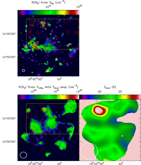
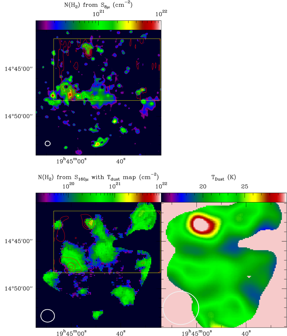
The corresponding H₂ column density map is shown in the upper panel of Fig. 7, which shows the H₂ distribution in NGC 6822 derived as above along with the CO(2–1) integrated intensity contours for the part observed by us in CO.

This way, we estimate the molecular gas mass within our observed zone to be ${\rm M(H_{2})\sim 6\times 10^{6}\ M_{\sun}}$ and about ${\rm M(H_{2})\sim 1\times 10^{7}\ M_{\sun}}$ over NGC 6822 as shown in Fig. 7. This is 20 – 25 times greater than using a Galactic value and is in excellent agreement with Israel (1997a) who estimated the total H₂ mass to be about $1.5\times 10^{7}$ M_☉.

We have also calculated the H₂ masses for the individual clouds in Table 2 using the 8${\rm\mu m}$ emission and the last column gives the corresponding estimated $N({\rm H}_{2})/I_{\rm CO(2-1)}$ values. The median and average values are 15 – 20 times the Galactic value, assuming a line ratio of 0.7 to go from $N({\rm H}_{2})/I_{\rm CO(2-1)}$ to . Overall, the agreement between the CO emission and the 8${\rm\mu m}$ based vision of where the molecular gas is found is quite good, suggesting that CO traces the H₂, albeit with a much higher factor than in the Galaxy. Galactic CO emission is present towards NGC 6822 (Israel 1997a) (see Sect. 10), the H I column is of course unaffected but the 8${\rm\mu m}$ continuum could be. However, since the morphology of the H₂ column density map resembles NGC 6822 so closely but not the local emission, we expect this contribution to be low.

6.4 Molecular gas mass from 160${\rm\mu m}$ emission

Figure 8: H₂ column density map estimated from $160{\rm\mu m}$ emission using the dust temperature map shown on the right (left), CO(2-1) intensity contours every $(0.15\mathrm{K}{\rm\ km\ s^{-1}})$ starting from $(0.15\mathrm{K}{\rm\ km\ s^{-1}})$. Temperature map from $160{\rm\mu m}$ Spitzer and $100{\rm\mu m}$ IRAS data (right) . The yellow rectangle is the region we have mapped in CO(2–1) with HERA. The beams for the NH₂, CO and temperature

are plotted in white.

We can perform the same sort of calculation based on the 160${\rm\mu m}$ emission, which we assume to come from dust grains large enough that they reach thermal equilibrium and are not affected by individual photons. The properties of the grains can be found in Li & Draine (2001) and Draine & Li (2007). The first step is to measure the dust temperature. Since the work by Israel (1997a), the Spitzer data for NGC 6822 has become available (Cannon et al. 2006), extending to longer wavelengths than IRAS and thus more sensitive to cool dust. Using the 70${\rm\mu m}$ and 160${\rm\mu m}$ Spitzer data, we derive, like Cannon et al. (2006), dust temperatures around 25 K (assuming that the dust cross-section varies with $\lambda^{-2}$). Since cool dust emits very weakly at 70 $\mu$m , we chose to use the 160${\rm\mu m}$ Spitzer and 100 ${\rm\mu m}$ IRAS data to better measure the temperature of the cool dust component. However, some of the 100${\rm\mu m}$ emission may still come from a warm component, causing an overestimate of the dust temperature of the cool component and a corresponding underestimate of the gas mass. NGC 6822 has an SED (Cannon et al. 2006, figure 12) similar to that of NGC 4414, as measured by the ISO LWS01 scan by Braine & Hughes (1999). In their Figure 4, they present a breakdown of the dust emission into warm and cool components. The 100 $\mu$m emission due to the warm dust is about 8% of the total 70 micron emission. In equation 7, we therefore take $\chi=0.08$ as our fiducial value but also test $\chi=0$ and $\chi=0.16$ to measure the effect of an error in $\chi$. We smoothed the 160${\rm\mu m}$ data to the resolution of the IRAS 100 $\mu$m HiRes maps ($118\arcsec\times 102\arcsec$). Assuming a modified grey-body law with a spectral index $\beta=2$ for the dust, we then estimate dust temperatures around 21K with Eq. 8 instead of 23K using the 70 and 160 $\mu$m data for the same regions. Changing $\chi$ from 0 to 0.08 causes a 0.3K change in dust temperature.

$$S_{100\mu m_{cool}}=S_{100\mu m}-\chi S_{70\mu m}$$ (7)

$$T_{dust}=f\left(\frac{S_{100\mu m_{cool}}}{S_{160\mu m}}\right)$$ (8)

The computed dust temperature map is shown at the right of Figure 8. The temperature map does not cover the whole galaxy because it was necessary to clip the very low signal-to-noise regions. Cuts were applied at 4 MJy/sr for both the 100 and 160 $\mu$m maps, leaving the odd shape seen in Figure 8. From the dust temperature, the HI column density, and the 160 $\mu$m emission, assumed optically thin, we can estimate the dust cross-section at 160 $\mu$m which can then be applied to regions with molecular gas.

Although the map of dust temperature is at IRAS resolution, we apply it to the full resolution 160 $\mu$m data so that the morphology is better reproduced. Smoothing does not affect the total 160 $\mu$m flux. Averaging the HI/160mu ratio map over regions with high enough 160 emission that the noise has little effect (4 MJy/sr) and low enough 160 emission to exclude regions where molecular gas will be present (8 MJy/sr), we obtain dust cross-section at 160 $\mu$m of $\sigma_{160}=5.1\times 10^{-26}$cm² per H-atom. We also varied the threshold values (from 4–8 to 6–12), this lead to a variation of sigma of at most 10%.

Cannon et al. (2006) found consistent values of Mdust/MHI for the individual regions they observed and some of the scatter is certainly attribuable to the molecular gas that they could not measure, although in most cases the HI dominates. They found a factor  5 lower ratio when they calculated Mdust/MHI for the whole galaxy. Using the 70/160 dust temperature like Cannon and the 160 micron emission, but only over the area where we felt we could reliably estimate the dust temperature (cuts at 1 MJy/sr at 70 $\mu$m and 4 MJy/sr at 160 $\mu$m , both smoothed to the 160 $\mu$m resolution) we find a dust cross-section (equivalent to Mdust/MHI ratio) of $4.7\times 10^{-26}$ cm² per H-atom with little variation, unlike Cannon et al. (2006).

Assuming a linear dependence of $\sigma_{160}$ on metallicity (Oxygen abundance), a solar oxygen abundance of $12+log(O/H)=8.67$ (Asplund et al. 2005), $12+log(O/H)=8.11$ in NGC 6822 (Lee et al. 2006), and a solar metallicity dust cross-section of $\sigma_{160}=2.25\times 10^{-25}$cm² per H-atom (Table 6 of Li & Draine 2001), we obtain $\sigma_{160}=6.3\times 10^{-26}$cm² per H-atom for NGC 6822. Thus, our “observational” results are in good agreement with model calculations.

Using this temperature map and the cross-section $\sigma_{160}=5.1\times 10^{-26}$cm² per H-atom above, the total H column density at each position is

$${\rm N_{Htot}}=S_{160\mu m}\frac{1}{\sigma_{160_{\mu m}}\ B_{{160\mu m},{\rm T_{d}}}}$$ (9)

so that the H₂ column density is simply

$${\rm N_{H_{2}}}=\frac{1}{2}({\rm N_{Htot}}-{\rm N_{{H\textsc{I}}}})$$ (10)

The left panel of Fig. 8 shows the total H₂ column density derived in this way using an ${\rm N_{{H\textsc{I}}}}$ map smoothed to the 160$\mu$m 40$\arcsec$ resolution.

In Table 2 the H₂ mass estimates for individual clouds are only based on the 8${\rm\mu m}$ map due to angular resolution – the 160 $\mu$m data is at a resolution larger than the clouds. Tables 3 and 4, which provide a summary of the molecular gas mass calculations, include the 160 $\mu$m results.

It is very difficult to estimate uncertainties for our mass estimates. Statistical noise related errors, as manifested by the variations within “blank” areas of maps, are about $10^{20}$ in column density. Systematic uncertainties are certainly present as well so we consider the column density noise in our maps to be $\sim 2\times 10^{20}$ H₂ cm^-2.

6.5 The $N({\rm H}_{2})/I_{\rm CO(2-1)}$ ratio in NGC 6822

We have estimates of the CO-to-${\rm H_{2}}$ conversion factor on two different scales, at the cloud level and for the whole area mapped by HERA in CO(2–1).

Table 3: Average over the cloud sample of the $N({\rm H}_{2})/I_{\rm CO(2-1)}$ factor for the different methods used to derive the molecular gas mass.

Method		$\left<N({\rm H}_{2})/I_{\rm CO(2-1)}\right>$	Range
		${\rm cm^{-2}/K{\rm\ km\ s^{-1}}}$	${\rm cm^{-2}/K{\rm\ km\ s^{-1}}}$
${\rm 8\mu m}$	by eye	$2.1\pm 0.8\times 10^{21}$	$0.3-4.3\times 10^{21}$
	CPROPS	$3.5\pm 1.4\times 10^{21}$	$1.0-6.4\times 10^{21}$
${\rm 160\mu m\mbox{ with }}$	by eye	$1.5\pm 0.9\times 10^{21}$	$0.5-3.1\times 10^{21}$
${\rm T_{dust}\mbox{ map }}$	CPROPS	$1.3\pm 0.9\times 10^{21}$	$0.4-2.7\times 10^{21}$
${\rm M_{vir}}^{\mathrm{}}$	by eye	$1.6\pm 0.8\times 10^{21}$	$0.2-2.8\times 10^{21}$
	CPROPS	$1.1\pm 0.8\times 10^{21}$	$0.07-3.5\times 10^{21}$

Averages for the “by eye” and CPROPS methods are respectively over 11 and 9 clouds. In the case of the virial masses the number of clouds in the sample are 12 and 11 respectively for the “by eye” and CPROPS methods (see Table 2).

Table 4: Molecular gas masses, $N({\rm H}_{2})/I_{\rm CO}$ conversion factor and characteristic time to transform molecular gas into stars derived from IR emission.

	total ${\rm M_{H_{2}}}$	map ${\rm M_{H_{2}}}$	$N({\rm H}_{2})/I_{\rm CO}$	$\tau$
	${\rm M_{\sun}}$	${\rm M_{\sun}}$	${\rm\frac{cm^{-2}}{{K{\rm\ km\ s^{-1}}}}}$	yr
${\rm 8\mu m}$	$9.2\times 10^{6}$	$5.7\times 10^{6}$	$5.3\times 10^{21}$	$2.2\times 10^{8}$
$160{\rm\mu m}$	${4.6\times 10^{6}}$	$3.4\times 10^{6}$	$2.3\times 10^{21}$	$1.3\times 10^{8}$

The second column refers to the area mapped in CO. The last column is the inverse of the SFE.

Table 3 presents averages and total ranges of the $N({\rm H}_{2})/I_{\rm CO(2-1)}$ factor for our sample of clouds for the different methods we have used. The average is over 9 clouds in the case of CPROPS and 14 in the case of the “by eye” identification. For the virial mass the average is over our full sample of 11 and 15 clouds using a projected area as defined in Sec. 4.2.1. We have included the virial mass as a valid method to estimate cloud masses because the size-linewidth relationship we find (see Fig. 4) is similar to the one for Galactic clouds. This suggests that the CO molecules are not greatly photodissociated at the outer edge of the clouds and that the cloud size as determined from the CO emission is close to the true size of the molecular clouds. As might be expected in this case, the masses computed by the virial theorem are similar to but usually lower than the ones we estimate by the other methods (see Table 2).

We find similar values of $N({\rm H}_{2})/I_{\rm CO(2-1)}$ for the different methods used, around 1.5–$2\times 10^{21}\,{\rm cm^{-2}/(K{\rm\ km\ s^{-1}})}$, 5–10 times the $\approx 2\times 10^{20}\,\,{\rm cm^{-2}/(K{\rm\ km\ s^{-1}})}$ value for the inner part of the Milky Way in CO(1–0) (e.g. Dickman et al. 1986). From interferometric CO data Bolatto et al. (2008) using only virial masses for a sample of dwarf galaxies of the Local Group find a value of the CO-to-${\rm H_{2}}$ factor similar to the Galactic value despite the low metallicities. Presumably this is because they detect the dense protected parts of bright clouds.

There has been evidence for a long time that as the size scale increases, at least for low metallicity objects, the $N({\rm H}_{2})/I_{\rm CO}$ factor increases as well (Rubio et al. 1993). Table 4 shows the mass estimates for the area of NGC 6822 mapped by HERA and a larger region including the HERA map and which covers virtually all of the stellar and H$\alpha$ emission. The $N({\rm H}_{2})/I_{\rm CO(2-1)}$ factors and characteristic times to transform molecular gas into stars are shown in columns 3 and 4 for the different methods used to estimate the molecular gas column density. After subtraction of the HI column density, some pixels became negative; we have attributed a nil value to the pixels in the N${\rm H_{2}}$ map where the molecular gas column density had a negative value after application of Eq. 4. The $N({\rm H}_{2})/I_{\rm CO(2-1)}$ factor for the whole of the area mapped in CO(2–1) is slightly larger ($\sim 5\times 10^{21}\,\,{\rm cm^{-2}/(K{\rm\ km\ s^{-1}})}$) than for the individual clouds and 20–25 times larger than the standard Galactic value for the molecular ring of the Milky Way. This higher value is close to the 4 – 8 $\times 10^{21}\,\,{\rm cm^{-2}/(K{\rm\ km\ s^{-1}})}$ found by Israel (1997a) for scales of $\sim 50\arcsec$. We now turn to modeling to better understand the relationship between CO emission, H₂ mass, and the other properties of the clouds.

7 Modeling the CO emission from NGC 6822 GMCs

Figure 9: Model $N{\rm(H_{2})}/I_{\rm{C\textsc{I}}}$ (top) and $N({\rm H}_{2})/I_{\rm CO}$ factors as a function of visual extinction A_v and H column density into the cloud. As the atomic Hydrogen skin is very thin even for the highest UV field used here, the clouds are essentially completely molecular so the depth is shown as H₂ depth not H. The $x-$axis extends beyond standard cloud column densities in order to show how a change in cloud structure with respect to Galactic clouds would affect the CO intensities. The expected range is roughly indicated by a box in the lower panel. While the UV field has little effect on the Hydrogen, it has a major effect on the C⁺/C/CO transition.

Figure 10: Line strengths of the major observables C II, O I, C I, and CO as a function of visual extinction A_v and H column density into the cloud. Lines are as in Fig. 8 – black for density $n=1000$, red for the nominal $n=10000$ with CLOUDY default rates, and green for $n=10000$ with UMIST rates. The solid, dashed, and dotted lines are for respectively UV fields of 1, 10, and 100 times the estimated solar neighborhood value.

7.1 Description of the models

We have modeled the structure and the emission of the molecular clouds in NGC 6822 using CLOUDY version 07.02 (Ferland et al. 1998). CLOUDY computes the spectrum of a gaseous nebula using as only inputs the geometry, the gas and dust composition and the energy input on the nebula. Originally designed to deal with photoionized nebula, CLOUDY is now able to perform accurate calculations in the Photo Dissociation Region (PDR) and even well into the molecular clouds due to the implementation of the H₂ physics (Shaw et al. 2005) and a network of 1000 reactions involving 68 molecules (Abel et al. 2005). CLOUDY determines steady-state solutions for the chemistry and predicts the emission in the fine structure lines and CO, which are the main coolants in the PDR and the molecular cloud.

The exact geometry of the regions to be modeled, the position of the excitation sources and the shape of the incident continuum are not well known. Therefore we have performed plane-parallel models with the incident continuum determined by Black (1987) for the local interstellar radiation field (ISRF). This continuum is not restricted to the FUV range as in many classical PDR calculations. To estimate the intensity of the incident continuum we have taken into account that according to Draine et al. (2007), the gas in NGC 6822 is exposed to a minimum radiation field of order twice the local ISRF. On the other hand, the variation in the GALEX FUV observations of NGC 6822 is about a factor 50 from the general field to the stronger fields around specific positions. Therefore, we have computed simulations for scaled versions of the local ISRF by factors of 1, 10, and 100. However, most of the clouds in our regions of interest are exposed to (GALEX-based) fields of less than 10. In addition to the Black (1987) continuum, the calculations include the cosmic microwave background and a cosmic-ray ionization rate of $2.5\ 10^{-17}$s^-1, which is typical of the Milky Way (Williams et al. 1998) but not known for NGC 6822. Given that UV photons penetrate further into molecular clouds in the low-metallicity environment of NGC 6822 than into their Galactic counterparts, the cosmic ray flux is not as critical a parameter.

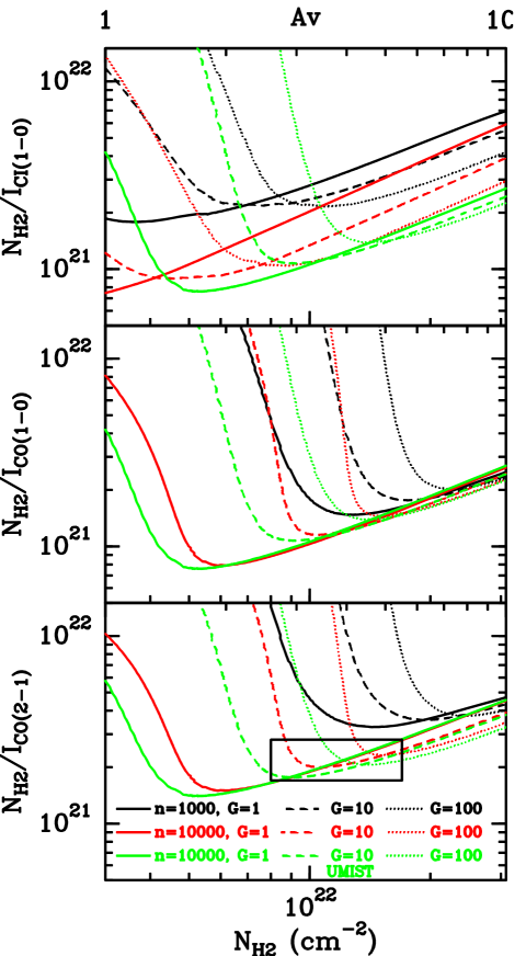
We have adopted typical gas abundances and dust distributions (including PAHs) of the Milky Way interstellar medium (see CLOUDY documentation for the exact values). These abundances are scaled using the metallicity of NGC 6822 (0.3 solar). The simulations have been computed for two densities, 1000 and 10000 mol cm^-3, which are representative of the bulk of the molecular gas. In addition we have computed simulations with two series of rate coefficients – the CLOUDY default and the UMIST. The reason for testing two sets of rate coefficients is that in the comparison of PDR codes (Röllig et al. 2007), the C I–CO transition was found to vary significantly (from $A_{v}\sim 2$ to $A_{v}\sim 5$) depending largely on these coefficients. This is a critical region for low-metallicity molecular clouds because the CO emission depends strongly on the fraction of the cloud in which CO has formed.

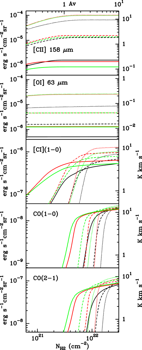
In summary, we have explored a grid of 12 models (3 fields $\times$ 2 densities $\times$ 2 reaction rates). In all the simulations, a line width of 2 km/s is included via the turbulence command. The results are summarized in Figs. 9 and 10. In both figures, the simulation results are shown for three radiation fields, solid lines for $G_{0}=1$, dashed for $G_{0}=10$ and dotted for $G_{0}=100$ (where $G_{0}$ is the intensity of the far ultraviolet continuum in the cloud surface in units of the Habing (1968) field). The red and black curves use the CLOUDY default rate coefficients for respectively densities of $10^{4}$ and $10^{3}$ cm^-3. The green curve uses the UMIST rate coefficients for $10^{4}$ cm^-3.

The range of H₂ column densities explored goes from $\sim 3\ 10^{21}$ cm^-2 to $\sim 3\ 10^{22}$ cm^-2. Assuming that the grain abundance scales with metallicity, those column densities correspond to visual extinctions ($A_{v}$) from 1 to 10. Therefore, the model simulations cover the full range of H₂ column densities expected in the region of interest, from a few $10^{21}$ cm^-2 of the extended component derived from the dust emission to $\sim 10^{22}$ cm^-2 towards the center of the molecular clouds detected in CO (see Fig. 7). The latter value is also typical for molecular clouds in the Milky Way (Larson 1981), although regions of higher column density also exist, particularly towards cloud cores and GMC centers.

Among the goals of the modelling is to see if the $N({\rm H}_{2})/I_{\rm CO}$ factor is close to our other estimates and to predict testable fluxes in other important cooling lines which could then act as further diagnostics. Figure 9 shows the $N({\rm H}_{2})/I_{\rm CO}$ and $N({\rm H}_{2})/I_{\rm{C\textsc{I}}}$ ratios as a function of the total column density and visual extinction into the cloud for all models. In other words, at a given depth into the cloud the plotted $N({\rm H}_{2})/I_{\rm CO}$ and $N({\rm H}_{2})/I_{\rm{C\textsc{I}}}$ ratios are the integrated values from the cloud surface to that cloud depth. While, Fig. 10 shows the cumulated intensity for different lines as as a function of the total column density into the cloud.

The column densities shown in Figs. 9 and 10 are actually total (H + H₂) but the gas is almost completely molecular due to the low radiation fields (the model with a highest atomic H fraction has only 3 $\%$ of H in the region of interest).

The C I to CO transition occurs when the lines in Fig. 9 are decreasing steeply due to the fact that CO begins to emit strongly just after formation. This is clearer in the two lower panels of Fig. 10, which shows how the energy emitted is divided into the principal PDR cooling lines: CO, C I, C II, and O I[63]. The models suggests that no CO emission is expected for H₂ column densities below $\sim 2$ 10²¹ cm^-2.

7.2 Constraining the physical conditions and the $N({\rm H}_{2})/I_{\rm CO}$ ratio

Currently, the spectral data available to study NGC 6822 is limited to HI and CO. However, in this section we will try to constrain the physical conditions and the $N({\rm H}_{2})/I_{\rm CO}$ ratio using our model calculations and assuming line ratios typical of normal galaxies. In doing so, we will also make use of GALEX measurement of the far-UV field in NGC 6822 (Draine et al. 2007). We will also take into account our previous estimations of the H₂ column density of the CO clouds detected in NGC 6822. The exact value is not important since we show below that the $N({\rm H}_{2})/I_{\rm CO}$ conversion factor depends weakly on NH2 in the region of interest. Therefore, the $N({\rm H}_{2})/I_{\rm CO}$ conversion factor derived in this section remains independent of other previous estimations.

For normal spiral galaxies, the C II[158] integrated intensities in energy units are typically 1000 – 2000 times the CO(1-0) intensity (Stacey et al. 1991; Braine & Hughes 1999). On the other hand, the O I[63] to C II[158] ratio is $\sim 0.3$ in normal galaxies at large scales (Braine & Hughes 1999; Lord et al. 1996; Malhotra et al. 2001) and can be even higher when studying smaller scales as the spiral arms of M31 (Rodriguez-Fernandez et al. 2006). These are lower limits to the O I/C II ratios in the neutral components of the ISM since a fraction of the observed C II emission may come from ionized gas not closely associated with molecular clouds or PDRs.

The simulations show that the C II flux varies linearly with the incident field and depends little on the density for the range explored here, as expected. The O I flux depends strongly on both density and radiation field and for the low density models the flux is well below the large-scale value of 1/3 that of the C II typical of normal galaxies. Thus, a density of 10⁴ cm^-3 is more appropriate to reproduce the O I/C II ratio.

Even for large column densities where the CO is formed for all the parameters studied, the simulations predict strong variations in the C II/CO(1-0) ratio from 100 to $10^{4}$ for incident field of $G_{0}=1$ to 100 respectively. To reproduce ratios of 1000-2000 typical of normal spiral galaxies a relatively low intensity incident field of $G_{0}=10$ is favored. Similarly, the model C I/CO(1–0) ratio also favors low intensity fields since the predicted ratios are high, about 0.5 in K km/s except for $G=1$ with a ratio of about 0.3, whereas typical observed values are about 0.2 (e.g. Gerin & Phillips 2000) and often less. For lower columns or the late CO formation curves, the C I/CO ratio is substantially higher (due to the weak CO).

All together, the comparison of the model prediction with the typical line ratios yields a representative density of $\sim$ 10⁴ cm^-3 and incident field in the range 1–10, in agreement with Draine et al. (2007) and our GALEX estimates for NGC 6822. Taking into account those density and incident radiation fields, and a range of H₂ column densities from 8 10²¹ cm^-2 to 2 10²² cm^-2, which comprise the expected H₂ column density of the CO clouds detected in NGC 6822, a likely value for $N({\rm H}_{2})/I_{\rm CO(2-1)}$ is in the range $\sim 2-3\times 10^{21}\,{\rm cm^{-2}/(K{\rm\ km\ s^{-1}})}$. These estimations of the $N({\rm H}_{2})/I_{\rm CO(2-1)}$ factor do not depend critically on the exact H₂ column density of the molecular clouds in NGC 6822 and agree reasonably well with other estimations. Increasing the radiation field further pushes the CO edge of the cloud deeper in, probably unrealistically deep unless the molecular clouds in NGC 6822 have higher column densities than Galactic GMCs. Observing the C II, O I, and C I lines with the Herschel satellite would be of great interest because they are sensitive respectively to the SFR, the SFR and density, and the cloud depth (the others being independent of total cloud column density – cf. Fig. 10).

8 The efficiency of star formation in NGC 6822

Using the ${\rm H\alpha}$ luminosity and the calibration from Kennicutt (1998), Cannon et al. (2006) derive a global star formation rate of $0.015\,{\rm M_{\sun}\leavevmode\nobreak\ yr^{-1}}$. Israel et al. (1996) find $0.04\,{\rm M_{\sun}\leavevmode\nobreak\ yr^{-1}}$ over the last $10^{7}$ years from bolometric luminosity measurements. Using the calibration from Hunter & Gallagher (1986) which supposes that close to half of the ionizing photons are lost to dust and a Salpeter IMF:

$${\rm\dot{M}}=5\times 10^{-8}L(H_{\alpha})/L_{\sun}\leavevmode\nobreak\ {\rm M_{\sun}\leavevmode\nobreak\ yr^{-1}}$$ (11)

yields, with ${\rm L(H_{\alpha})}=2\times 10^{39}\leavevmode\nobreak\ {\rm erg\leavevmode\nobreak\ s^{-1}}$ (de Blok & Walter 2006b) a star formation rate of $0.026\,{\rm M_{\sun}\leavevmode\nobreak\ yr^{-1}}$; this is the value we will use for NGC 6822.
The star formation efficiency is usually defined as the ratio of the star formation rate over the mass of molecular gas available to form stars:

$${\rm SFE=\frac{SFR}{M_{H_{2}}}}$$ (12)

The characteristic time to transform molecular gas into star is directly $\tau={\rm 1/SFE}$. Table 4 shows the values of the characteristic time $\tau$ for the different methods used to estimate the molecular gas column density. The H₂ consumption times are smaller than those found for large spirals, about ${\rm 2\times 10^{9}\leavevmode\nobreak\ yr}$ (Murgia et al. 2002; Kennicutt 1998), such that the SFE in NGC 6822 is higher by the same ratio. This is consistent with the high star formation efficiency found by Gardan et al. (2007) in M 33, a spiral galaxy larger than NGC 6822 but an order of magnitude less luminous and less massive than the Milky Way. Two other small galaxies, IC10 and NGC 2403 (which is very similar to M33), have also been found to have high SFEs by respectively Leroy et al. (2006), Kennicutt (1998) and Blitz et al. (2007) but the constraints on the $N({\rm H}_{2})/I_{\rm CO}$ conversion are not stringent.

Going to $z\sim 1$, the star formation rate increases by at least one order of magnitude (Madau et al. 1996; Wilkins et al. 2008). Even if the gas fraction was higher in the past, a high star formation efficiency has to be introduced in order to explain such a wide variation of the star formation rates. Small Local Group galaxies such as NGC 6822, M 33, the LMC or the SMC share some properties with intermediate redshift objects: they are gas rich, have subsolar metallicities and seem to exhibit high star formation efficiencies. Low-luminosity NGC 6822 also shares with early universe objects a high FIR/CO luminosity ratio. Note that both CO and the dust emission are affected by metallicity. However, unlike these rare but very luminous galaxies, NGC 6822 (like the other small local objects above) has a low SFR, placing it in an empty region of Figures 8 and 9 in Solomon & Vanden Bout (2005). High spatial resolution observations of these local systems may help us understand the physics of intermediate redshift galaxies.

9 Hubble X and Hubble V

9.1 Diffuse CO emission South of Hubble X

Figure 11: CO(2-1) and H I spectra of the region south of of Hubble X in which CO emission appears to be detected (cf. Fig. 6). The solid line is the CO(2–1) summed over a 2.57 arcmin² region east of Hubble X, the dotted line is the H I spectrum summed over the same region, and the dashed line is a JCMT CO (2–1) spectrum taken at RA $19^{\mathrm{h}}42^{\mathrm{m}}19\ \aas@@fstack{s}7$, Dec $-14\degr 50\arcmin 31\arcsec$.

Table 5: Properties of the H II regions Hubble V and Hubble X.

Name	$\left.\alpha_{\mathrm{off}}\right.^{\mathrm{a}}$	$\left.\delta_{\mathrm{off}}\right.^{\mathrm{a}}$	${\rm T_{CO\ mb}}$	${\rm I_{CO}}$
	$\arcsec$	$\arcsec$	mK	${\rm K{\rm\ km\ s^{-1}}}$
Hubble V	$-68.5$	$299.0$	500	$0.93$
Hubble X	$55.2$	310.8	$\left.<85\right.^{\mathrm{b}}$	$\left.<0.19\right.^{\mathrm{c}}$

• Offsets with respect to the reference position$(\alpha_{o},\delta_{o})=(19^{\mathrm{h}}44^{\mathrm{m}}57\ \aas@@fstack{s}8,-14\degr 48\arcmin 11\arcsec)$

• Corresponding to a $3\sigma$ level

• Corresponding to a $3\sigma$ level and a $3{\rm\ km\ s^{-1}}$ fwhm linewidth.

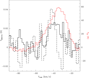
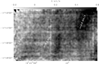
A major question is whether large quantities of H₂ could be missed through the use of CO as a tracer of molecular gas. In particular, does the presence of the luminous star forming region Hubble X (see Table 5 for positions of Hubble V and X) with copious H$\alpha$, FUV, 160$\mu$m and 8$\mu$m emission but without a CO detection invalidate CO as a tracer of H₂ in galaxies like NGC 6822? As shown in Fig. 7, for reasonable estimates of the radiation field or dust temperature, the dust emission corresponds to that expected from the atomic component alone. Thus, we believe that towards the H II region there is in fact very little H₂, and not just little CO. However, we see evidence for “diffuse” CO emission from the H I-rich region near and South of Hubble X (see Fig. 11).

In Fig. 11, we have summed the CO and H I spectra over a region roughly $50\arcsec\times 200\arcsec$ in size, yielding an apparent detection in CO despite the absence of individual clouds with detectable CO emission. Also shown is the result of an observation towards $19^{\mathrm{h}}42^{\mathrm{m}}19\ \aas@@fstack{s}7$, $-14\degr 50\arcmin 31\arcsec$ made with the JCMT in CO(2–1) at $21\arcsec$ resolution in 1992, which, although the signal-to-noise ratio is low, seems to show CO emission towards roughly the same position and at the same velocities. With the resolution available in extragalactic observations, “diffuse” signifies that neither spatially nor spectrally can we distinguish the clouds which, taken together over a large area, appear to contribute a detectable CO signal. While these clouds could be like Galactic cirrus, our resolution and brightness sensitivity are not sufficient to be sure. They are not like either galactic GMCs or the individual clouds discussed in Sections 4. Using the methods described in Sect. 6, no H₂ is found in this area although the CO luminosity is $\sim 10^{4}$ K km/s pc².

9.2 The ¹³CO and HCN emission in Hubble V

Figure 12: Spectra of the Hubble V (Hubble 1925) H II region. (dotted line)  CO divided by 10, (continous line)  CO, (black) $\mathrm{J}=2\rightarrow 1$, (red) $\mathrm{J}=1\rightarrow 0$.

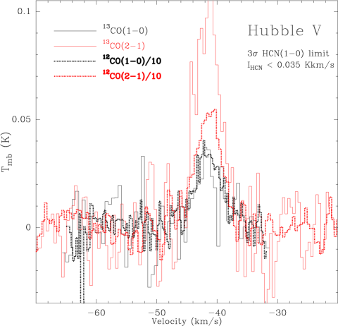
Unlike most spiral galaxies (Braine et al. 1993), comparing the CO(1–0) emission with the CO(2–1) emission convolved to $21\arcsec$ angular resolution yields a line ratio of about ${\rm{CO(2-1)}/{CO(1-0)}\sim 1.2}$ in Hub V. This is unlikely to be the case over much of NGC 6822 because rather warm and dense gas is required, including some optically thin emission. The $\@element[13]{\mathrm{C}}$O emission confirms this for Hubble V – the $\@element[12]{\mathrm{C}}$O/$\@element[13]{\mathrm{C}}$O ratio is 15 in the (1–0) transition but only 5.7 in the (2–1) transition, showing that the higher transition is efficiently excited. Israel et al. (2003a) found considerably higher $\@element[12]{\mathrm{C}}$O/$\@element[13]{\mathrm{C}}$O line ratios with the SEST telescope. This is a strong indication for the presence of tenuous molecular gas with low CO optiocal depths surrounding the Hubble V cloud, probably similar to the diffuse gas found near Hubble X (see Sect. 9.1)

In order to estimate the fraction of dense gas in Hubble V, we observed the HCN(1–0) line at 88.6316 GHz. HCN has a high dipole moment and thus requires high densities to be excited. HCN(1–0) was not detected despite reaching a $3\sigma$ noise level of 0.035 K km s^-1, a factor 60 below the CO(1-0) line. Typical values of CO(1–0)/HCN(1–0) are $\sim 50$ in galactic disks (Kuno & Nakai 1997, for M 51, Braine et al. 1997, for NGC 4414, Brouillet et al. 2005, for M 31), 10 – 20 in nuclei (Nguyen et al. 1992; Henkel et al. 1991), and less in ultraluminous infrared galaxies which are as a result believed to have a particularly high fraction of their H₂ in dense cores (Gao et al. 2007). Again with the SEST, Israel et al. (2003a) reports detection of the HCO⁺(1–0) line in Hubble V, at 4 times the brightness of our limit to HCN(1–0). While rather extreme, Brouillet et al. (2005) noted an apparent rise in the HCO⁺/HCN ratio going towards the outskirts of M31, where the metallicity presumably decreases. From the data presented in this paper, despite being a major H II region, Hubble V is not particularly rich in dense gas. If the CO underestimates the H₂ mass in Hubble V, then the dense gas fraction in Hubble V is lower than in spiral disks because the HCN in dense cores should be less affected by the dissociating radiation field than the CO.

10 Galactic emission

A factor which greatly complicates studies of NGC 6822 is the presence of a Galactic molecular cloud along the line-of-sight towards NGC 6822. Some optical/UV emission is absorbed and the cloud emits at (at least) FIR wavelengths, making it difficult to clearly identify the emission coming from NGC 6822. This is particularly a question at 160$\mu$m where the dust temperature apparently decreases to the West but this is likely due to the increasing column density and low temperature of the Galactic cloud. In CO, the Galactic cloud can be separated from NGC 6822 (see Fig. 13) so that we know the western part is more affected. A velocity gradient from roughly East to West is present in the cloud, in addition to the column density gradient. For a cloud distance of 100 pc, realistic due to the $-20\degr$ galactic latitude of NGC 6822, the resolution is about 1500 a.u. or 0,007 pc, making this one of the highest-resolution observations up to now of a local cloud. A dedicated study of the large scale structure of this Galactic cirrus cloud will be presented by Israel et al. (in prep). Figure 13 shows where FIR emission and optical/UV absorption are most expected. The decrease in dust temperature at the NW corner of the 160$\mu$m map in Fig. 8 might be due to the cirrus. However, from looking at the region around RA 19:44:32 Dec -14:45:00, it is clear that any emission from the cirrus falls below our intensity cuts, whether at 100 or 160$\mu$m.

Figure 13: CO(2–1) emission from the local molecular “cirrus” cloud along the line of sight to NGC 6822. Indicated on the figure are the velocities of the emission at 3 different positions.

11 Conclusions

From large-scale CO mapping of a very nearby low metallicity galaxy, we identify a sample of molecular clouds, most of which were also detected by the CPROPS algorithm, allowing an unbiased assessment of their properties. The properties of these GMCs (size, linewidth, virial mass) appear similar to Galactic clouds but the H₂ mass per CO luminosity is much higher such that we estimate $N({\rm H}_{2})/I_{\rm CO(2-1)}\approx 2\times 10^{21}\,{\rm cm^{-2}/(K{\rm\ km\ s^{-1}})}$ for the clouds. A variety of methods yield coherent values. Our modeling with the CLOUDY program also provides similar ratios for reasonable parts of parameter space. At large scales ($\sim$ kpc, well above that of the clouds), we find evidence for a higher $N({\rm H}_{2})/I_{\rm CO}$, $\sim 4\times 10^{21}\,{\rm cm^{-2}/(K{\rm\ km\ s^{-1}})}$ , in agreement with work in NGC 6822 by Israel (1997a) and in the SMC by Rubio et al. (1993). No evidence for H₂ in the absence of CO emission was found. The molecular gas masses derived using the high $N({\rm H}_{2})/I_{\rm CO}$ values estimated here, coupled with an ${\rm SFR=0.026\,M_{\sun}\,yr^{-1}}\pm 50\%$, support the idea that molecular gas is more quickly cycled into stars in these small low metallicity galaxies. In turn, this appears coherent with our image of rapid star formation in intermediate redshift galaxies.