An effective field theory approach to two trapped particles

Abstract

We discuss the problem of two particles interacting via short-range interactions within a harmonic-oscillator trap. The interactions are organized according to their number of derivatives and defined in truncated model spaces made from a bound-state basis. Leading-order (LO) interactions are iterated to all orders, while corrections are treated in perturbation theory. We show explicitly that next-to-LO and next-to-next-to-LO interactions improve convergence as the model space increases. In the large-model-space limit we regain results from a pseudopotential. Arbitrary scattering lengths are considered, as well as a generalization to include the non-vanishing range of the interaction.

I Introduction

Much experimental progress has recently been achieved in the area of ultra-cold atoms. It is now possible kohl to make systems of atoms confined in optical lattices formed by laser beams and at the same time control the strength of the two-body interaction with magnetic fields. The atoms are cooled down to extremely low temperatures and, in the limit of low tunneling, each lattice site may be regarded as a harmonic-oscillator (HO) well, which is independent from the others and contains only a few atoms. Using a Feshbach resonance, the two-body interaction can be fine-tuned so that the $S$-wave scattering length $a_{2}$ is made much larger than the range $R$ of the interaction. By doing so, the theoretical problem of a system of trapped particles interacting via short-range forces can be realized experimentally.

Such atomic systems present remarkable similarities to some nuclear physics systems. Indeed, the two-nucleon scattering length is much larger than the range of the nuclear force, set by the pion mass. In such a situation, the physical properties of few-body systems are universal, that is, they depend mainly on $a_{2}$, not on the details of the two-body interaction. At sufficiently low energies, an effective field theory (EFT) has been formulated which turns this separation of scales into an expansion in powers of $R/a_{2}$ aleph . Except for isospin, which does play a role in the relative relevance of few-body forces, the version of this EFT used in nuclear physics nukeEFTrev is formally indistinguishable from the theory describing atomic systems Braat . (Nevertheless, the underlying theories for the two cases are very different.) As a consequence, atomic systems characterized by large scattering lengths can be studied with techniques developed in nuclear physics and, conversely, provide an excellent testing ground for few- and many-body methods that can be further applied, with little or no change, to the description of nuclear systems at low energies.

The no-core shell model (NCSM) is one of the most flexible ab initio methods used to obtain the solution to the non-relativistic Schrödinger equation for many-nucleon systems tradNCSM . Currently, it is the only such method able to reach medium-mass nuclei with no restrictions to closed or nearly-closed shells and at the same time to handle local and non-local interactions on the same footing. It uses a discrete single-particle basis —typically a HO basis— and, being a numerical method, relies on a suitable truncation of the model space accessible to nucleons —in the form of a maximum number $N_{max}$ of accessible shells above the minimum configuration. This requires the use of effective interactions (not only among nucleons but also among nucleons and external probes such as photons, when they are present) to account for effects left out by the truncation to a finite model space. The method of choice has been the construction of effective operators via unitary transformations. This involves the use of an approximation, the so-called “cluster approximation”, which is not a priori controlled, and which poses challenges for the description of low-momentum observables ncsm:eff_op . An alternative is to use EFT to construct effective interactions that are consistent with the underlying theory of QCD directly in the model spaces where many-nucleon calculations are carried out NCSM .

In this paper, we consider the problem of two trapped atoms with large scattering length, $|a_{2}|\gg R$, from the perspective of EFT interactions solved with the NCSM. The main simplification with respect to the nuclear case is that the trapping potential provides a natural single-particle basis; its HO length $b$ does not need to be removed at the end of the calculation because it represents the long-distance physics of the trap. As long as $b\gg R$, the trapped system should still exhibit universal behavior, although for $b\hskip 1.99997pt\raisebox{2.15277pt}{$<$}\raisebox{-3.00003pt}{$\sim$}\hskip 1.99997pt|a_{2}|$ it is significantly different from that of the untrapped system.

We use EFT techniques to expand the interaction between particles as a series of contact interactions with an increasing number of derivatives, and calculate energy levels inside the trap by explicitly solving the Schrödinger equation. We extend here the work initiated in Ref. trap0 , in which only the leading-order (LO) interaction was investigated. We include explicitly corrections up to the next-to-next-to-leading-order (N²LO), and show how they provide improved convergence as $N_{max}$ increases, at least as long as they are treated in perturbation theory. Finite and infinite values of the scattering length $a_{2}$ are considered, and we show that in the $N_{max}\to\infty$ limit our LO results converge to the levels of a pseudopotential pseudo with the same scattering length, obtained by Busch et al. HT . Starting at NLO a finite value of the effective range $r_{2}$ is allowed as well, and at higher orders other effective-range expansion parameters could be included similarly. The $N_{max}\to\infty$ limit of our subleading-order EFT provides a derivation of the generalized Busch et al. relation models ; DFT_short ; mehen . With the two-body system thus understood, we can use our method to calculate the energies of larger trapped systems usnext .

Other approaches to the same problem of course exist in the literature. They are frequently based on a specific form for the interparticle potential (see, for example, Ref. models ). Closest in spirit to ours is probably the approach alhassid where an effective short-range interaction is fitted to several levels of the pseudopotential at unitarity, but diagonalized exactly. What distinguish our framework are its i) systematic character, in the form of a controlled expansion; and ii) generality, since no assumptions about the form of the short-range interactions are needed. These features allow the same method to apply across fields. Of course, the low-energy observables themselves should be in agreement among different approaches, as long as they are calculated properly.

The paper is organized as follows. We first show in Sec. II the general formalism of our approach, including a detailed description of the treatment beyond leading order. We illustrate the method in different situations (finite and infinite scattering length, negligible and non-vanishing effective range, etc.) in Sec. III. We conclude and discuss future applications in Sec. IV. Appendices A, B, and C provide some of the details omitted in the main text.

II General Considerations

We consider a non-relativistic system of two particles of reduced mass $\mu$ that interact with each other in the $S$ wave. For definiteness, we think of two-component fermions, which support a single $S$ channel and interact also in $P$ and higher waves, but the framework can be straightforwardly applied to bosons and other fermions. In free space, the properties of this system can be characterized by scattering phase shifts for each partial wave of angular momentum $l$ at relative on-shell momentum $k$, $\delta_{l}(k)$. When the relative momentum is much smaller than the inverse of the range $R$ of the interparticle interaction, $k\ll 1/R$ (we use units in which $\hbar=1$ and $c=1$), the phase shifts are given by the effective range expansion (ERE); for example, in the $S$ wave,

$$k\,\cot\delta_{0}(k)=-\frac{1}{a_{2}}+\frac{1}{2}r_{2}k^{2}+\frac{1}{4}P_{2}k^{4}+\ldots,$$ (1)

where $a_{2}$, $r_{2}$, $P_{2}$, $\ldots$ are, respectively, the scattering length, effective range, shape parameter, and higher ERE parameters not shown explicitly. A similar expansion exists for $P$ and higher partial waves.

Generically, the sizes of ERE parameters are set by $R$, for example $|r_{2}|\sim R$. The ERE (1) is an expansion in powers of $kR$. Given a desired precision, the ERE can be truncated and the system described by a finite number of parameters. Potentials that generate the same values for this finite number of ERE parameters cannot be distinguished at this precision level: they all generate the same wavefunction for distances beyond the range of the force, $r\hskip 1.99997pt\raisebox{2.15277pt}{$>$}\raisebox{-3.00003pt}{$\sim$}\hskip 1.99997ptR$. Such potentials are said to belong to the same universality class. Most interesting is the case where the depth of the interaction potential is fine-tuned so that an $S$-wave bound state is near threshold and the associated scattering length is large, $|a_{2}|\gg R$. Then the physics of the bound state is largely independent of the potential; for example, for $R\ll r\ll a_{2}$ the wavefunction of a state of energy $E$ is

$$\psi(\vec{r})\propto\frac{1}{r}\left\{1-\left[1-\mu a_{2}r_{2}E+\ldots\right]\frac{r}{a_{2}}+{\cal O}\left(\frac{r^{2}}{a_{2}^{2}}\right)\right\}.$$ (2)

Physics in the unitarity limit, $|a_{2}|\to\infty$, is controlled by the zero-energy bound state and exhibits a higher degree of universality.

The ERE description is useful because it is model independent. However, it does not directly provide a basis for the study of many-body systems. This can be accomplished using the ideas of EFT nukeEFTrev ; Braat . Since at low momenta the details of the interaction cannot be resolved, we can expand the interparticle interaction $V$ as a Taylor series in momentum space, as done in App. A; in coordinate space,

$$V(\vec{r}\,^{\prime},\vec{r}) = C_{0}\delta(\vec{r}\,^{\prime})\delta(\vec{r})-C_{2}\left\{\left[\nabla\,^{\prime 2}\delta(\vec{r}\,^{\prime})\right]\delta(\vec{r})+\delta(\vec{r}\,^{\prime})\left[\nabla^{2}\delta(\vec{r})\right]\right\}$$ (3)

$$+C_{4}\left\{\left[\nabla\,^{\prime 4}\delta(\vec{r}\,^{\prime})\right]\delta(\vec{r})+\delta(\vec{r}\,^{\prime})\left[\nabla^{4}\delta(\vec{r})\right]+2\left[\nabla\,^{\prime 2}\delta(\vec{r}\,^{\prime})\right]\left[\nabla^{2}\delta(\vec{r})\right]\right\}+\ldots$$

where $C_{0}$, $C_{2}$, and $C_{4}$ are parameters, and “…” denote interactions that contribute at higher orders. Because the interactions are singular, an ultraviolet (UV) cutoff $\Lambda$ has to be introduced to solve the Schrödinger equation. In order for observables to be independent of $\Lambda$ (renormalization-group invariance), the parameters $C_{i}$ have to depend on $\Lambda$. This is merely a consequence of the fact that the UV cutoff is an arbitrary separation between the short-range dynamics included explicitly in the dynamics (through high virtual momenta) versus that included implicitly in the potential (through its parameters).

Contributions to observables obtained from $V$ (3) can also be organized in powers of $kR$. It has, in fact, been shown aleph that in the two-body sector the EFT expansion reproduces the ERE (1) at each power of $kR$. In the generic situation, one can simply treat the whole potential in perturbation theory. When $|a_{2}|\gg R$, however, the $C_{0}$ term in Eq. (3) needs to be solved exactly, while the remaining terms can still be accounted for in perturbation theory aleph . These higher-order terms represent range and subtler effects in the $S$ wave, and $P$ and higher waves.

Here we are interested in the large-scattering-length scenario, when the two particles are trapped in an HO potential of frequency $\omega$. The HO introduces a third scale, the length $b=1/\sqrt{\mu\omega}$. In the relative frame, the Hamiltonian for this system reads

$$H=\frac{\omega}{2}\left[-b^{2}\nabla^{2}+\frac{r^{2}}{b^{2}}\right]+V.$$ (4)

As long as $b\gg R$, details of the interparticle potential remain irrelevant and universality is not destroyed. In the following we consider various values for the ratio $b/a_{2}$, which are, as discussed in Sec. I, of interest in both atomic and nuclear physics.

We want to set up a perturbative approach; we thus write the Hamiltonian (4) for the relative motion as

$$H=H^{(0)}+V^{(1)}+V^{(2)}+\ldots,$$ (5)

with the energy and wavefunction decomposed accordingly,

$$|\psi\rangle=|\psi^{(0)}\rangle+|\psi^{(1)}\rangle+|\psi^{(2)}\rangle+\ldots,$$ (6)

and

$$E=E^{(0)}+E^{(1)}+E^{(2)}+\ldots$$ (7)

The superscript ⁽ⁿ⁾ corresponds to the order in perturbation theory of the different terms. Here we order interactions according to the power counting of Ref. aleph and for convenience we split the parameters $C_{i}$ in Eq. (3) among different orders.

The leading-order (LO) Hamiltonian is

$$H^{(0)}=\frac{\omega}{2}\left[-b^{2}\nabla^{2}+\frac{r^{2}}{b^{2}}\right]+C_{0}^{(0)}\delta(\vec{r}),$$ (8)

and the corresponding wavefunction $\psi^{(0)}(\vec{r})$ is the solution of the Schrödinger equation

$$\left(H^{(0)}-E^{(0)}\right)\psi^{(0)}(\vec{r}) = 0.$$ (9)

The next-to-leading-order (NLO) correction to the potential is

$$V^{(1)}=C_{0}^{(1)}\delta(\vec{r})-C_{2}^{(1)}\left\{\left[\nabla^{2}\delta(\vec{r})\right]+2\left[\vec{\nabla}\delta(\vec{r})\right]\cdot\vec{\nabla}+2\delta(\vec{r})\nabla^{2}\right\},$$ (10)

and the first-order corrections to the energy, $E^{(1)}$, and to the wavefunction, $\psi^{(1)}(\vec{r})$, are obtained in first-order perturbation theory. That is, they are such that

$$\left(H^{(0)}-E^{(0)}\right)\psi^{(1)}(\vec{r}) = \left(E^{(1)}-V^{(1)}\right)\psi^{(0)}(\vec{r}).$$ (11)

The next-to-next-to-leading-order (N²LO) correction to the potential $V^{(2)}$ is given by

$$V^{(2)} = C_{0}^{(2)}\delta(\vec{r})-C_{2}^{(2)}\left\{\left[\nabla^{2}\delta(\vec{r})\right]+2\left[\vec{\nabla}\delta(\vec{r})\right]\cdot\vec{\nabla}+2\delta(\vec{r})\nabla^{2}\right\}$$ (12)

$$+C_{4}^{(2)}\left\{\left[\nabla^{4}\delta(\vec{r})\right]+4\left[\vec{\nabla}\nabla^{2}\delta(\vec{r})\right]\cdot\vec{\nabla}+4\left[\vec{\nabla}\vec{\nabla}\delta(\vec{r})\right]\cdot\cdot\vec{\nabla}\vec{\nabla}\right.$$

$$\left.\qquad\quad+4\left[\vec{\nabla}\delta(\vec{r})\right]\cdot\vec{\nabla}\nabla^{2}+2\delta(\vec{r})\nabla^{4}\right\}.$$

The corrections $E^{(2)}$ and $\psi^{(2)}(\vec{r})$ are obtained from

$$\left(H^{(0)}-E^{(0)}\right)\psi^{(2)}(\vec{r}) = \left(E^{(2)}-V^{(2)}\right)\psi^{(0)}(\vec{r})+\left(E^{(1)}-V^{(1)}\right)\psi^{(1)}(\vec{r}),$$ (13)

which just means perturbation theory to first order in $V^{(2)}$ and to second order in $V^{(1)}$. Extension to higher orders is straightforward.

We work on a basis of HO wavefunctions $\phi_{nlm}(\vec{r})$ with energies $E_{nl}=(2n+l+3/2)\omega\equiv(N+3/2)\omega$. Useful properties of these wavefunctions are summarized in App. B. In the HO basis the singularity of the potential (3) can be tamed by imposing a maximum number of shells $N_{max}$ NCSM , which corresponds to a UV momentum cutoff

$$\Lambda=\frac{1}{b}\sqrt{2N_{max}+3}.$$ (14)

We therefore expand the wavefunction (6) in the HO basis in the finite space,

$$\psi^{(\nu)}(\vec{r})=\sum_{n,l=0}^{N_{max}}\sum_{m=-l}^{l}c_{nlm}^{(\nu)}\;\phi_{nlm}(\vec{r}),$$ (15)

where $c_{nlm}$ are coefficients to be determined.

Since the two-body potentials up to N²LO only support $S$ waves, to this order the eigenfunctions with $l>0$ are simply the HO wavefunctions $\phi_{nlm}(\vec{r})$ with eigenvalues $(2n+l+3/2)\omega$ up to the energy $(N_{max}+3/2)\omega$. For $l=0$, on the other hand, the levels are affected by the interparticle potential. Denoting by $n_{max}$ the maximum value of the radial quantum number (that is, $n_{max}$ is the largest integer smaller than, or equal to, $N_{max}/2$) and omitting the labels $l=0$ and $m=0$, the $S$ wavefunction can be written as

$$\psi^{(\nu)}_{0}(r)=\sum_{n=0}^{n_{max}}c_{n}^{(\nu)}\phi_{n}(r)$$ (16)

in terms of the HO $S$ wavefunctions $\phi_{n}(r)\equiv\phi_{n00}(\vec{r})$,

$$\phi_{n}(r) = \pi^{-3/4}b^{-3/2}\left[L_{n}^{(1/2)}\left(0\right)\right]^{-1/2}e^{-r^{2}/2b^{2}}L_{n}^{(1/2)}\left(r^{2}/b^{2}\right),$$ (17)

where $L_{n}^{(\alpha)}$ is the generalized Laguerre polynomial.

The resulting energies (7) will depend on $N_{max}$ as well as $\omega$, $E=E(N_{max},\omega)$. Since $N_{max}$ is arbitrary, we want the energies not to depend sensitively on $N_{max}$. This cannot be achieved in general, but it can for the shallow levels of interest —that is, those with $E\hskip 1.99997pt\raisebox{2.15277pt}{$<$}\raisebox{-3.00003pt}{$\sim$}\hskip 1.99997pt{\cal O}(1/2\mu R^{2})$, which are dominated by physics at distances $r\hskip 1.99997pt\raisebox{2.15277pt}{$>$}\raisebox{-3.00003pt}{$\sim$}\hskip 1.99997ptR$. As we show in the following, this is accomplished by allowing the $C_{i}^{(\nu)}$ to depend on both $N_{max}$ and $\omega$, $C_{i}^{(\nu)}=C_{i}^{(\nu)}(N_{max},\omega)$. Nevertheless, at any order a residual $N_{max}$ dependence introduces an error in the calculation of shallow levels, which should be proportional to powers of $1/\Lambda$. At the end of the calculation we want to take $N_{max}$ sufficiently large, $\Lambda\hskip 1.99997pt\raisebox{2.15277pt}{$>$}\raisebox{-3.00003pt}{$\sim$}\hskip 1.99997pt1/R$, so that this error is not larger than the error proportional to powers of $R$ stemming from the truncation of Eq. (3).

II.1 LO renormalization

The physics at LO is obtained by diagonalizing the two-body Hamiltonian (8). The approach is similar to the treatment in a free-particle basis aleph , with the difference that we work here only with bound states, which naturally are closely related to HO states because of the presence of the trap. Renormalization of the interaction at LO has already been discussed in Ref. trap0 , but for completeness we repeat the derivation here.

We start with the Schrödinger equation (9) for the wavefunction of the two-fermion system, $\psi^{(0)}(\vec{r})$. One can show, by inserting Eq. (16) into Eq. (9) and projecting on a HO basis state $\phi_{n}(r)$, that the expansion coefficients are given by

$$c_{n}^{(0)}=\kappa^{(0)}\frac{\phi_{n}(0)}{E^{(0)}-(2n+3/2)\omega},$$ (18)

where $\kappa^{(0)}=C_{0}^{(0)}\psi^{(0)}(0)$ is itself a combination of the unknown coefficients. Direct substitution of the expansion coefficients back into Eq. (16) yields

$$\psi^{(0)}_{0}(r) = \frac{\kappa^{(0)}\mu}{2\pi^{3/2}b}\exp{(-r^{2}/2b^{2})}\sum_{n=0}^{n_{max}}\frac{L_{n}^{(1/2)}(r^{2}/b^{2})}{\frac{E^{(0)}}{2\omega}-(n+\frac{3}{4})}.$$ (19)

From the consistency condition at $r=0$ we obtain the relation trap0 that an energy $E^{(0)}$ has to satisfy:

$$\frac{1}{C_{0}^{(0)}(n_{max},\omega)} = \frac{\mu}{2\pi^{3/2}b}\sum_{n=0}^{n_{max}}\frac{L_{n}^{(1/2)}(0)}{\frac{E^{(0)}}{2\omega}-(n+\frac{3}{4})}$$ (20)

$$= -\frac{2\mu}{\pi^{2}b}\left\{\frac{\Gamma\left(n_{max}+\frac{3}{2}\right)}{\Gamma\left(n_{max}+1\right)}\left[1+R\left(n_{max},\frac{E^{(0)}(\omega)}{2\omega}\right)\right]-\frac{\pi}{2}\frac{\Gamma\left(\frac{3}{4}-\frac{E^{(0)}(\omega)}{2\omega}\right)}{\Gamma\left(\frac{1}{4}-\frac{E^{(0)}(\omega)}{2\omega}\right)}\right\},$$

where

$$R\left(m,\frac{\varepsilon}{2}\right) = \frac{1-2\varepsilon}{8(m+1)\left(m+\frac{7}{4}-\frac{\varepsilon}{2}\right)}$$ (21)

$$\;{}_{3}F_{2}\left(1,m+\frac{3}{2},m+\frac{7}{4}-\frac{\varepsilon}{2};m+2,m+\frac{11}{4}-\frac{\varepsilon}{2};1\right)$$

in terms of the generalized hypergeometric function ${}_{3}F_{2}$. (In Eq. (20) we used Eqs. (78) and (79).) Finally, the constant $\kappa^{(0)}$ is fixed by the chosen normalization of $\psi^{(0)}_{0}(r)$. (It can be calculated using Eq. (80).) Note that this constant is energy dependent; when necessary we denote it by $\kappa^{(0)}_{E^{(0)}}$.

The rhs of Eq. (20) clearly depends on $n_{max}$ and $\omega$, and so does $C_{0}^{(0)}$. In a given model space, the coupling constant $C_{0}^{(0)}$ can be fixed to reproduce one observable, in this case one energy of the two-body system. If, to be definite, we take that energy as the ground-state energy in the trap,

$$E^{(0)}_{0}=E_{0}(\omega),$$ (22)

then $C_{0}^{(0)}(n_{max},\omega)$ is determined from

$$\frac{1}{C_{0}^{(0)}(n_{max},\omega)} = -\frac{2\mu}{\pi^{2}b}\left\{\frac{\Gamma\left(n_{max}+\frac{3}{2}\right)}{\Gamma\left(n_{max}+1\right)}\left[1+R\left(n_{max},\frac{E_{0}(\omega)}{2\omega}\right)\right]-\frac{\pi}{2}\frac{\Gamma\left(\frac{3}{4}-\frac{E_{0}(\omega)}{2\omega}\right)}{\Gamma\left(\frac{1}{4}-\frac{E_{0}(\omega)}{2\omega}\right)}\right\}.$$ (23)

While one energy in the spectrum is fixed in all model spaces, the rest of the energy spectrum runs with the model space: the remaining energies $E^{(0)}_{i\geq 1}=E^{(0)}_{i\geq 1}(n_{max},\omega)$ satisfy Eq. (20) and in general depend not only on $\omega$ but also on $n_{max}$. These energies should converge as $n_{max}\to\infty$ to finite values $E^{(0)}_{i\geq 1}(\infty,\omega)$. However, once $\Lambda$ in Eq. (14) exceeds $1/R$, the theoretical errors are dominated by the physics of the effective range $r_{2}$, which was left out of LO.

II.2 Renormalization beyond LO

In the two-nucleon system, the effective range is much smaller than the scattering length, but is finite. In an atomic system near a Feshbach resonance, the range is usually neglected, although it should become relatively more important as one moves away from the resonance. In either case, the LO, which ignores the range, contains energy-dependent errors of ${\cal O}(k^{2}a_{2}R)$. In addition, in both cases, the truncation to a model space excludes physics of momenta beyond $\Lambda$, which introduces further energy-dependent errors of ${\cal O}(k^{2}a_{2}/\Lambda)$. In other words, the truncation induces contributions to the effective range, the shape parameter, and so on, governed by $\Lambda$ rather than by $1/R$. The role of contributions beyond LO is to correct for these two types of energy-dependent errors: NLO for $k^{2}$ errors and higher orders for higher powers of $k$.

In the untrapped system, the power counting for a system with a large $S$-wave scattering length $a_{2}$ is such that corrections beyond LO have to be treated as perturbations aleph . It is one of our goals in this paper to show that treating higher orders in perturbation theory in the presence of the trap allows for a systematic improvement of the two-body energies.

At NLO, we include corrections as first-order perturbations on top of the LO wavefunction $|\psi^{(0)}\rangle$. As discussed above, in LO we fix $C_{0}$ so that one of the states has the “observed” energy. The NLO correction in Eq. (3) introduces a new parameter $C_{2}$ that can be chosen so that a second energy level is fixed. However, the NLO term induces, in general, a non-vanishing correction to the energy used to fix $C_{0}$. One should, therefore, readjust $C_{0}$ so that in NLO we reproduce the two observables (energy levels) at the same time. In order to keep track of this change, it is convenient to split $C_{0}$ into an LO piece $C_{0}^{(0)}$, which remains unchanged, and an NLO piece $C_{0}^{(1)}$, as done in Eq. (10), and treat the latter in perturbation theory as well.

Thus, for energies we have

$$E^{(1)} = \langle\psi^{(0)}|V^{(1)}|\psi^{(0)}\rangle=\frac{\kappa^{(0)2}}{C_{0}^{(0)2}}\left\{C_{0}^{(1)}+4\mu C_{2}^{(1)}\left[E^{(0)}-\frac{C_{0}^{(0)}}{\pi^{3/2}b^{3}}\sum_{n=0}^{n_{max}}L_{n}^{(1/2)}(0)\right]\right\}$$ (24)

$$= \frac{\kappa^{(0)2}}{C_{0}^{(0)2}}\left\{C_{0}^{(1)}+4\mu C_{2}^{(1)}\left[E^{(0)}-\frac{4C_{0}^{(0)}}{3\pi^{2}b^{3}}\frac{\Gamma\left(n_{max}+\frac{5}{2}\right)}{\Gamma\left(n_{max}+1\right)}\right]\right\},$$

where we used Eq. (77).

The requirement that two energy levels have the correct positions in the spectrum fixes the amount of change from LO, thus providing two equations that determine the unknown coupling constants $C_{0}^{(1)}$ and $C_{2}^{(1)}$ in each model space. In the case when the lowest level $E_{0}$ is already fixed to a given (experimental or theoretical) value, $E_{0}^{(1)}=0$. However, in the case with finite non-negligible range, one can alternatively choose that in LO $C_{0}^{(0)}$ be fixed to a level of the two-body spectrum without a range, while in NLO that level is shifted to the correct position with range, thus requiring that $E_{0}^{(1)}\neq 0$. These two alternatives are the HO-basis equivalent to fixing $C_{0}^{(0)}$ in a free-particle basis to, respectively, a known binding energy (such as the deuteron binding energy) or the scattering length. In either case, if we take, say, the first excited level $E_{1}(\omega)$ to be reproduced at NLO in addition to the ground state, the two equations for the determination of $C_{0}^{(1)}(n_{max},\omega)$ and $C_{2}^{(1)}(n_{max},\omega)$ can be written as

$$E_{i}^{(1)}(n_{max},\omega)=E_{i}(\omega)-E_{i}^{(0)}(n_{max},\omega),\qquad i=0,1.$$ (25)

From Eqs. (24) and (25), we can easily solve for $C_{0}^{(1)}(n_{max},\omega)$ and $C_{2}^{(1)}(n_{max},\omega)$:

$$\frac{4\mu C_{2}^{(1)}}{C_{0}^{(0)2}}=\frac{E_{1}^{(1)}/\kappa^{(0)2}_{E_{1}^{(0)}}-E_{0}^{(1)}/\kappa^{(0)2}_{E_{0}^{(0)}}}{E_{1}^{(0)}-E_{0}^{(0)}}$$ (26)

and

$$\frac{C_{0}^{(1)}}{4\mu C_{2}^{(1)}}=\frac{4C_{0}^{(0)}}{3\pi^{2}b^{3}}\frac{\Gamma\left(n_{max}+\frac{5}{2}\right)}{\Gamma\left(n_{max}+1\right)}-\frac{E_{0}^{(0)}E_{1}^{(1)}/\kappa^{(0)2}_{E_{1}^{(0)}}-E_{1}^{(0)}E_{0}^{(1)}/\kappa^{(0)2}_{E_{0}^{(0)}}}{E_{1}^{(1)}/\kappa^{(0)2}_{E_{1}^{(0)}}-E_{0}^{(1)}/\kappa^{(0)2}_{E_{0}^{(0)}}}.$$ (27)

With these coupling constants fixed, Eq. (24) provides values for the other energy levels.

The form of the NLO wavefunction is a bit more complicated; in App. C we show that, up to higher-order terms,

$$\psi^{(0)}(r)+\psi^{(1)}(r) = \left(1+A^{(1)}\right)\frac{\kappa^{(0)}\mu}{2\pi^{3/2}b}e^{-r^{2}/2b^{2}}\sum_{n=0}^{n_{max}}\frac{L_{n}^{(1/2)}(r^{2}/b^{2})}{\frac{1}{2\omega}(E^{(0)}(n_{max})+E^{(1)}(n_{max}))-(n+\frac{3}{4})}$$ (28)

$$+2\mu\kappa^{(0)}\frac{C_{2}^{(1)}}{C_{0}^{(0)}}\sum_{n}\phi_{n}(0)\phi_{n}(r),$$

where

$$A^{(1)}=\kappa^{(0)2}\left[\frac{E^{(1)}}{\pi^{3/2}b^{3}}\sum_{m}\frac{L_{m}^{(1/2)}(0)}{(E^{0}-E_{m})^{3}}+2\mu\frac{C_{2}^{(1)}}{C_{0}^{(0)2}}\right].$$ (29)

Of course, just as in LO, the levels not used as input at NLO will have errors $\propto 1/\Lambda$. As we show explicitly later, the magnitude of these errors is smaller than at LO, since more physics has been accounted for. If further precision is desired, we can continue the procedure to higher orders.

In this paper we consider one order more, N²LO, so as to show the systematic trend of improvement —but we omit details that can be obtained straightforwardly, if painfully. The correction $E^{(2)}$ to the energy is obtained using perturbation theory up to the second order. In addition to the second-order correction from $V^{(1)}$ (10), one has the first-order correction from $V^{(2)}$ (12):

$$E^{(2)}=\langle\psi^{(0)}|V^{(2)}|\psi^{(0)}\rangle+\frac{1}{2}\left\{\langle\psi^{(0)}|V^{(1)}|\psi^{(1)}\rangle+\langle\psi^{(1)}|V^{(1)}|\psi^{(0)}\rangle\right\}.$$ (30)

The potential $V^{(2)}$ affects the energy levels that were fixed already, so again it is convenient to compensate for this by adding in Eq. (12) perturbative shifts $C_{0}^{(2)}$ and $C_{1}^{(2)}$ with respect to the lower-order parameters. These two parameters, together with the four-derivative parameter $C_{4}^{(2)}$, are determined so that three energy levels are fixed to the correct values. Taking the lowest three levels $E_{i}(\omega)$, $i=0,1,2$, to be fixed, the three equations for the determination of $C_{0}^{(2)}(n_{max},\omega)$, $C_{2}^{(2)}(n_{max},\omega)$, and $C_{4}^{(2)}(n_{max},\omega)$ are

$$E_{i}^{(2)}(n_{max},\omega)=E_{i}(\omega)-E_{i}^{(0)}(n_{max},\omega)-E_{i}^{(1)}(n_{max},\omega),\qquad i=0,1,2.$$ (31)

Obviously, higher corrections can be added in a similar fashion.

II.3 Infinite-cutoff limit

In the absence of a trap, the LO EFT is formally equivalent aleph in the infinite-cutoff limit to the pseudopotential pseudo . As we show here, the situation is the same in the presence of the HO potential, where the pseudopotential was solved in Ref. HT . We consider explicitly the EFT to NLO, in order to derive also the first corrections to the pseudopotential in the trap.

The wavefunction to NLO for a finite value of $n_{max}$ is given in Eq. (28). By having $n_{max}\to\infty$ and using Eq. (74) one obtains:

$$\psi(r) = -\left(1+A^{(1)}\right)\frac{\kappa^{(0)}\mu}{2\pi^{3/2}b}e^{-r^{2}/2b^{2}}\Gamma\left(\frac{3}{4}-\frac{\varepsilon(\infty)}{2}\right)U\left(\frac{3}{4}-\frac{\varepsilon(\infty)}{2},\frac{3}{2},\frac{r^{2}}{b^{2}}\right)$$ (32)

$$+2\mu\kappa^{(0)}\frac{C_{2}^{(1)}}{C_{0}^{(0)}}\delta(\vec{r}).$$

where $U$ is the confluent hypergeometric function, and we have introduced the energy

$$\varepsilon(\infty)=\frac{E^{(0)}(\infty,\omega)+E^{(1)}(\infty,\omega)}{\omega},$$ (33)

which is the limit of the energy (in units of $\omega$) of the two-body system in the trap. The second term in Eq. (32) was obtained by using the completeness of the HO basis,

$$\lim_{n_{max}\to\infty}\sum_{n=0}^{n_{max}}\phi_{n}(0)\phi_{n}(r)=\lim_{N_{max}\to\infty}\sum_{nl=0}^{N_{max}}\sum_{m=-l}^{l}\langle 0|nlm\rangle\langle nlm|\vec{r}\rangle=\delta(\vec{r}).$$ (34)

The singularity of this term is mitigated by the pre-factor $C_{2}^{(1)}/C_{0}^{(0)}$, which vanishes as $1/\Lambda$ for large cutoff. It stems from the enhancement of high virtual momenta due to the second derivatives in $V^{(1)}$. As shown in App. A, for an equivalent energy-dependent potential this term is absent.

For small, non-vanishing values of $r$, i.e. $0<r\ll b$, use of Eq. (76) gives

$$\psi(0<r\ll b)\propto\frac{1}{r}\left\{1-2\frac{\Gamma\left(\frac{3}{4}-\frac{\varepsilon(\infty)}{2}\right)}{\Gamma\left(\frac{1}{4}-\frac{\varepsilon(\infty)}{2}\right)}\frac{r}{b}+{\cal O}\left(\frac{r^{2}}{b^{2}}\right)\right\}.$$ (35)

By identification of this wavefunction with the wavefunction in the untrapped case, Eq. (2), we obtain the relation between the energy of the trapped two-body system and the ERE parameters:

$$\frac{\Gamma\left(\frac{3}{4}-\frac{\varepsilon(\infty)}{2}\right)}{\Gamma\left(\frac{1}{4}-\frac{\varepsilon(\infty)}{2}\right)}=\frac{b}{2a_{2}}\left\{1-\frac{a_{2}r_{2}}{b^{2}}\varepsilon(\infty)+\ldots\right\}.$$ (36)

In our framework, Eq. (36) is to be interpreted in perturbation theory. At LO only the scattering length is taken into account, and the energies $\varepsilon^{(0)}(\infty)$ are given by

$$\frac{\Gamma\left(\frac{3}{4}-\frac{\varepsilon^{(0)}(\infty)}{2}\right)}{\Gamma\left(\frac{1}{4}-\frac{\varepsilon^{(0)}(\infty)}{2}\right)}=\frac{b}{2a_{2}},$$ (37)

a relation first found in Ref. HT using the pseudopotential pseudo . The latter can be viewed as a renormalization of the delta-function interaction aleph . Indeed, the strength of the LO delta-function interaction has to decrease with the increase of the model-space size in order for it to give sensible results. One can see from Eq. (72) that for large $n_{max}$ the first term in Eq. (23) grows as $\sqrt{n_{max}}$. Taking the limit of Eq. (23) and using Eq. (37), one finds

$$C_{0}^{(0)} = -\frac{\pi^{2}}{\mu\Lambda}\left[1+\frac{\pi}{2\Lambda a_{2}}+{\cal O}\left(\frac{1}{\Lambda^{2}b^{2}}\right)\right].$$ (38)

In the $\Lambda b\to\infty$ limit this running is exactly the one found in free space aleph : the non-trivial rate of change with the cutoff $\Lambda$ is controlled by $1/a_{2}$. This is not surprising since the large-$\Lambda$ behavior should be independent of the long-range physics of the trap.

At NLO, the effective range appears: Eq. (36) becomes

$$\frac{\Gamma\left(\frac{3}{4}-\frac{\varepsilon^{(0)}(\infty)+\varepsilon^{(1)}(\infty)}{2}\right)}{\Gamma\left(\frac{1}{4}-\frac{\varepsilon^{(0)}(\infty)+\varepsilon^{(1)}(\infty)}{2}\right)}=\frac{b}{2a_{2}}\left\{1-\frac{a_{2}r_{2}}{b^{2}}\varepsilon^{(0)}(\infty)\right\},$$ (39)

which can be solved to this order as

$$\varepsilon^{(1)}(\infty)=\frac{2a_{2}r_{2}}{b^{2}}\frac{\varepsilon^{(0)}(\infty)}{\psi^{(0)}\left(\frac{3}{4}-\frac{\varepsilon^{(0)}(\infty)}{2}\right)-\psi^{(0)}\left(\frac{1}{4}-\frac{\varepsilon^{(0)}(\infty)}{2}\right)},$$ (40)

in terms of the digamma function $\psi^{(0)}$. In the presence of range, all levels change from LO to NLO. The range in fact controls the asymptotic behavior of the NLO coupling constants. In the large-$n_{max}$ limit we find from Eqs. (27) and (26) that

$$C_{0}^{(1)}=-\frac{\pi^{3}r_{2}}{12\mu}\left[1+{\cal O}\left(\frac{1}{r_{2}\Lambda},\frac{1}{a_{2}\Lambda}\right)\right]$$ (41)

and

$$\frac{C_{2}^{(1)}}{C_{0}^{(0)2}}=\frac{\mu r_{2}}{8\pi}\left[1+{\cal O}\left(\frac{1}{r_{2}\Lambda}\right)\right].$$ (42)

Again, this is the same running as in free space aleph , as it should be. Note that it qualitatively changes for $r_{2}=0$. In this case, $\varepsilon^{(1)}(\infty)=0$, which means, given our choice of levels to fix the coupling constants at NLO, that $E_{0}^{(1)}=0$ and $E_{1}^{(1)}={\cal O}(E_{1}^{2}/\Lambda)$. As a consequence the ratio of energies in Eq. (26) goes to $0$ as $\Lambda\to\infty$, and $\mu\Lambda C_{0}^{(1)}$ and $\mu\Lambda^{3}C_{2}^{(1)}$ approach constants.

At N²LO the power counting of Ref. aleph indicates that no new ERE term should be included. This is a reflection of the fact that a fine-tuning in $a_{2}$ does not in general lead to an enhancement in the shape parameter $P_{2}$: in order to go from $r_{2}k^{2}/2$ to $P_{2}k^{4}/4$ two orders are needed. Therefore at N²LO Eq. (36) is unmodified. It is only at N³LO that we need to account for a non-vanishing $S$-wave shape parameter, also with an $S$-wave potential of the form of Eq. (12) (but with different parameters). For fermions, N³LO also contains a $P$-wave interaction to account for the $P$-wave scattering volume.

It is clear that the procedure can be continued to higher orders, and we expect for $l=0$ levels

$$\frac{\Gamma\left(\frac{3}{4}-\frac{\varepsilon(\infty)}{2}\right)}{\Gamma\left(\frac{1}{4}-\frac{\varepsilon(\infty)}{2}\right)}=-\frac{bk}{2}\cot\delta_{0}(k),$$ (43)

where

$$kb=\sqrt{2\varepsilon(\infty)}$$ (44)

and $\delta_{0}(k)$ is given by the ERE (1). This extension to subleading orders agrees with Refs. models ; DFT_short ; mehen . Waves with $l\geq 1$ can also be examined with the same method we developed here, but we leave details for future work.

The importance of Eq. (36) lies in the link between the energies inside the HO well, $\varepsilon(\infty)$, and the scattering parameters, $a_{2}$, $r_{2}$, etc. It is the analog of Lüscher’s formula luescher , which links the levels inside a cubic box and the same scattering parameters. As such, Eq. (36) provides the energy levels necessary to fix the coupling constants in finite model spaces when the ERE parameters are known. In the nuclear case, for example, the scattering parameters have been determined from data, so Eq. (36) can be used to fix the parameters of the pionless EFT without relying on a fit to nuclear levels, as done in Ref. NCSM . An extension of Ref. NCSM to this case is in progress.

In the atomic case, the lowest energy $E_{0}(\omega)$ of two trapped particles has been measured kohl . One can use $E_{0}(\omega)$ directly as input in Eq. (23). Alternatively, this energy was found kohl to be in good agreement with the lowest state of the theoretical spectrum obtained under a pseudopotential assumption HT , in which the eigenvalues are determined by the scattering length $a_{2}$. In Ref. trap0 we used this theoretical LO energy as input; we confirmed that the two-fermion spectrum of the underlying pseudopotential is reached asymptotically as $n_{max}\to\infty$, and we calculated the properties of three- and four-fermion systems. In subleading orders, we can now include effective range and higher effects, which might account for the small discrepancies kohl between the theory and experiment.

We should stress that, because the bare coupling constants are not observables, their sizes have no direct physical meaning. What matters is the total contribution of a given order to an observable. For example, for $\Lambda\hskip 1.99997pt\raisebox{2.15277pt}{$>$}\raisebox{-3.00003pt}{$\sim$}\hskip 1.99997pt1/r_{2}$, $C_{0}^{(0)}\hskip 1.99997pt\raisebox{2.15277pt}{$<$}\raisebox{-3.00003pt}{$\sim$}\hskip 1.99997ptC_{0}^{(1)}$, and yet, the NLO energy shift (40) is small as long as $r_{2}$ is sufficiently small. We show explicit results for energies in the next section.

III Results

In this section, we illustrate the approach described above in a few cases of interest for atomic and nuclear systems. We initially consider situations where the range of the interaction can be neglected; we first look at the unitarity limit, $b/a_{2}=0$, and then finite $b/a_{2}$. Finally, we consider the case where the range of the interaction is non-negligible albeit still small with respect to the scattering length. In all cases, we use Eq. (36) to provide the asymptotic levels in the trap.

III.1 Unitarity limit

We start by considering a system of two trapped particles at unitarity, characterized by $b/a_{2}=0$ and $r_{2}/b=0$. In the untrapped case, this situation can be realized by considering an attractive potential given by, for instance, a square well with a fine-tuned depth. Asymptotically, the wavefunction at zero energy behaves as $1/r$ and the scattering length $a_{2}$ is then infinite.

In the presence of the harmonic trap, the only scale is set by $b$, or, equivalently, $\omega$, so the solutions of Eq. (36) have to be constants; indeed, they are given by the poles of the Gamma functions in the denominators, i.e.,

$$\varepsilon_{n}(\infty)=\frac{1}{2}+2n,$$ (45)

where $n\geq 0$ is an integer. At each order we use a finite number of these energies to determine the interaction parameters in each model space: $\varepsilon_{0}$ at LO, $\varepsilon_{0}$ and $\varepsilon_{1}$ at NLO, and $\varepsilon_{0}$, $\varepsilon_{1}$, and $\varepsilon_{2}$ at N²LO.

Using the ground-state energy to determine $C_{0}^{(0)}$, Eq. (23) simplifies to

$$C_{0}^{(0)}(n_{max},\omega)=-\frac{\pi^{2}b}{2\mu}\frac{\Gamma\left(n_{max}+1\right)}{\Gamma\left(n_{max}+\frac{3}{2}\right)},$$ (46)

which at large cutoff becomes

$$\mu\Lambda C_{0}^{(0)}=-\pi^{2}\left[1+{\cal O}\left(\frac{1}{\Lambda^{4}b^{4}}\right)\right].$$ (47)

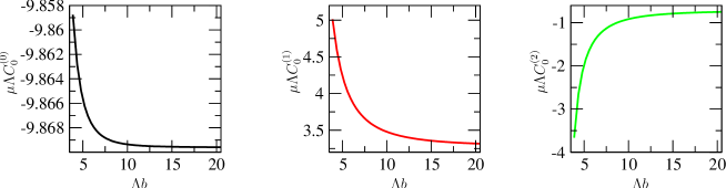
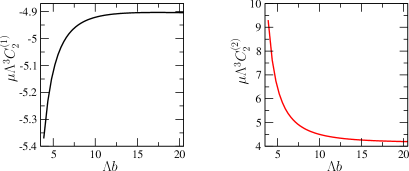
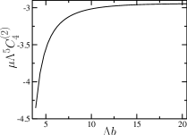
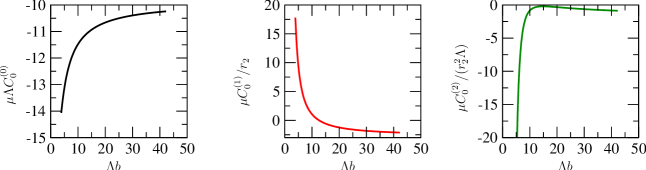
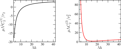
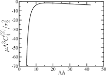
Analogous expressions can be derived for the other coupling constants. The resulting running of the coupling constants is shown in Figs. 1, 2, and 3. One can see that, in agreement with Sec. II.3, a coupling constant $C_{i}$ behaves asymptotically as $1/\Lambda^{2i+1}$.

Figure 1: The coupling constants $\mu\Lambda C_{0}^{(0)}$, $\mu\Lambda C_{0}^{(1)}$, and $\mu\Lambda C_{0}^{(2)}$ at unitarity as a function of the cutoff in the dimensionless combination $\Lambda b$.

Figure 2: The coupling constants $\mu\Lambda^{3}C_{2}^{(1)}$ and $\mu\Lambda^{3}C_{2}^{(2)}$ at unitarity as a function of the cutoff in the dimensionless combination $\Lambda b$.

Figure 3: The coupling constant $\mu\Lambda^{5}C_{4}^{(2)}$ at unitarity as function of the cutoff in the dimensionless combination $\Lambda b$.

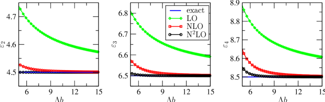
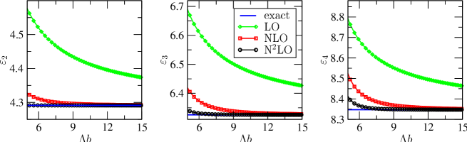
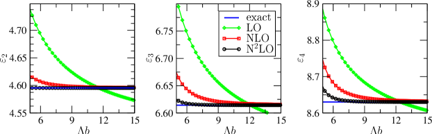
With the interaction parameters so determined, we calculate the remaining energies, which depend on $n_{max}$. Results for some excited states, from the second ($n=2$) to the fourth ($n=4$), are shown in Fig. 4 for different values of the cutoff $n_{max}$ in the dimensionless combination $\Lambda b$. At LO and NLO, all states change with $\Lambda b$; at N²LO, the second excited-state energy is used as input. As we showed in Sec. II.3, these calculated energies converge as $n_{max}$ increases to the values given in Eq. (45). The plot explicitly shows, in addition, that the convergence with respect to $n_{max}$ to the exact value is increased as higher-order corrections are added in perturbation theory.

Figure 4: Running with the dimensionless cutoff $\Lambda b$ of the second ($\varepsilon_{2}$), third ($\varepsilon_{3}$), and fourth ($\varepsilon_{4}$) excited-state energies, in units of $\omega$, for two particles in a trap with the interaction characterized by $b/a_{2}=0$ and $r_{2}/b=0$. Results at LO (green diamonds), NLO (red squares), and N²LO (black circles) are compared with the exact values (blue solid lines) given by Eq. (36). The coupling constants are fixed so that the ground-state, additionally the first excited-state, and additionally the second excited-state energies are reproduced in LO, NLO, and N²LO, respectively. (Note that, indeed, at N²LO the second excited state in the leftmost panel is constant on top of the exact value for all values of $\Lambda b$.)

In order to further study the effects of a finite $n_{max}$, we consider Eq. (36) from a different angle. Hitherto, we have used it simply to fix observables (energy levels). Now we employ it also to extract phase shifts. In a given model space, characterized by a given $n_{max}$, we calculate the energy levels $\varepsilon_{n}(n_{max})$. The lowest levels used in the fitting of coupling constants are, of course, exact, while all others deviate from the exact values. The momentum $k_{n}$ associated with an energy level $\varepsilon_{n}(n_{max})$ is

$$k_{n}b=\sqrt{2\varepsilon_{n}(n_{max})},$$ (48)

so that the phase shifts for discrete values of $k$, $\delta_{0}(k_{n})$, can be determined by simply inverting Eq. (43):

$$k_{n}b\cot\delta_{0}(k_{n})=-2\frac{\Gamma(3/4-\varepsilon_{n}(n_{max})/2)}{\Gamma(1/4-\varepsilon_{n}(n_{max})/2)}.$$ (49)

This allows us to study the effect of the truncation in a HO basis in terms of the more familiar ERE parameters: any deviation from the value $kb\cot\delta_{0}(k)=0$ is due to truncation errors and we can calculate the induced range, shape parameter, and so on. In Fig. 5, we plot $kb\cot\delta_{0}(k)$ in a model space with $n_{max}=15$ as a function of $k^{2}b^{2}$. (It is more natural to express $k$ in units of $1/a_{2}$, but at unitarity $b$ provides the only length unit.) At LO, $kb\cot\delta_{0}(k)$ starts off linear in $k^{2}b^{2}$: a linear fit (indicated by the dashed line) shows an induced effective range of about $0.17b$ in this particular model space. At larger values of $k^{2}b^{2}$ deviation from the linear behavior is seen, indicating the presence of further induced ERE parameters. NLO and N²LO corrections reduce the size of the ERE parameters, so that the results for the phase shifts improve order by order, getting closer and closer to the horizontal axis. Since here $\Lambda^{2}b^{2}=63$, at $k^{2}b^{2}\sim 60$, the errors are dominated by the higher orders, and therefore the lower orders do little to improve on the previous orders. However, at low momentum, the results systematically improve, as expected.

Figure 5: $S$-wave scattering phase shifts $kb\cot\delta_{0}(k)$ as function of the dimensionless squared momentum $k^{2}b^{2}$ in the finite model space characterized by $n_{max}=15$, at unitarity. The points at LO (green circles), NLO (red squares), and N²LO (black diamonds) are obtained from calculated energies via Eq. (49). The dashed line corresponds to a linear fit of the LO curve at small $kb$ values. For comparison, we also show results with the NLO potential fully diagonalized (black stars).

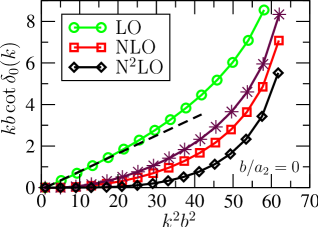
Our perturbative treatment thus provides a way to systematically reduce the effect of truncation to a reduced model space, demanded in the calculation of larger systems. Emboldened by this success, one might be tempted to treat the subleading potentials exactly in the Schrödinger equation. Apart from the renormalization problems pointed out in Ref. aleph , we find no obvious numerical improvement when this is done here. In Fig. 5 we also show for comparison results obtained when the NLO correction to the potential is not considered as a perturbation but fully diagonalized together with the LO potential. (The same two lowest levels are used to fix the two coupling constants of the LO+NLO potential.) One can see that by considering the LO+NLO potential this way, results are further away from the exact curve than by treating the NLO potential as a perturbation. This result is not particular to this example; more generally, truncation errors get worse when subleading corrections are treated improperly. The reason is that doing so includes only part of the higher-order corrections; it neglects the rest, needed to ensure systematic improvement.

III.2 Finite scattering length and zero range

In the previous subsection we saw that the rate of approach to the asymptotic values of two-body energies improves systematically as the order increases at unitarity. We now show that there are no qualitative changes when we consider the case of a pseudopotential away from unitarity HT , where the scattering length $a_{2}$ is finite, with $r_{2}$ still vanishing.

The corrections to the potential are taken into account as in the unitarity case, i.e., the LO correction is iterated to all orders whereas higher corrections are treated as perturbations. The parameters at each order are adjusted so that the lowest levels satisfy Eq. (36) exactly. The $\Lambda$ dependence of coupling constants is similar to unitarity, except for a markedly slower convergence for $C_{0}$. This is particularly obvious for $C_{0}^{(0)}$, when we compare the more general Eq. (38), which applies here, with its unitarity version (47).

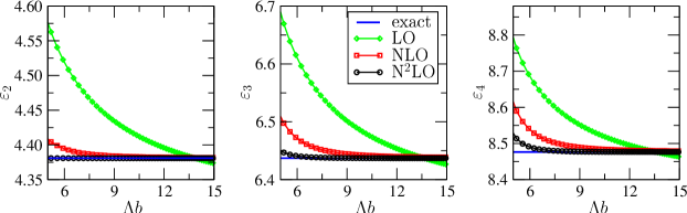
As for energies, let us first consider $a_{2}<0$. This situation corresponds to the case when the depth of the potential between the two particles is decreased starting from the fine-tuned value at unitarity. As an example, we show in Fig. 6 results for $b/a_{2}=-1$ for the same energy levels previously displayed at unitarity in Fig. 4. The exact values are slightly higher than at unitarity. As before, convergence of the energies to the exact values is improved as more corrections to the potential are added, and the difference between the truncated-space energy and the exact result is mitigated as more corrections are included.

Figure 6: Same as in Fig. 4, but for $b/a_{2}=-1$.

For a weak enough potential, $|a_{2}|$ becomes small. The energies are then close to the HO energies,

$$\varepsilon_{n}=\frac{3}{2}+2n+\delta\varepsilon_{n},$$ (50)

where $\delta\varepsilon_{n}$ is a small correction and $n=0,1,\ldots$. By using Eq. (36) and expanding the Gamma function around its poles one finds

$$\delta\varepsilon_{n}(\omega)=-\frac{4}{\Gamma\left(-\frac{1}{2}-n\right)P_{n}}\frac{a_{2}}{b}\left[1+{\cal O}\left(\frac{a_{2}}{b}\right)\right],$$ (51)

where

$$P_{n}=\lim_{z\to-n}\left[(z+n)\Gamma(z)\right]^{-1}=\left(1+\frac{1}{n}\right)^{n}\prod_{m=1,m\neq n}^{\infty}\left(1+\frac{1}{m}\right)^{n}\left(1-\frac{n}{m}\right).$$ (52)

We have verified numerically that in this case convergence to the exact value can even be sped up by considering all interactions as perturbations, as in the “natural” continuum case discussed in Ref. aleph .

We now turn to the case where $a_{2}>0$. As the interaction between particles becomes stronger (starting from the case at unitarity) the scattering length $a_{2}$ decreases. The ground state can have negative energy. The plot of the energy for excited states (starting from the second) for $b/a_{2}=1$ is shown in Fig. 7. The exact values are now slightly lower than at unitarity. Again, there is no qualitative change in the pattern of convergence with respect to unitarity or negative $a_{2}$.

Figure 7: Same as in Fig. 4, but for $b/a_{2}=1$.

For a strong enough interaction, the absolute value of the ground-state energy, $|\varepsilon_{0}(\infty)|$, is large and in the trapped system we have

$$\frac{\Gamma(3/4-\varepsilon_{0}(\infty)/2)}{\Gamma(1/4-\varepsilon_{0}(\infty)/2)}=\sqrt{-\frac{\varepsilon_{0}(\infty)}{2}}\left[1+{\cal O}\left(\varepsilon_{0}^{-2}(\infty)\right)\right].$$ (53)

Using Eq. (36), we find

$$\varepsilon_{0}(\infty)=-\frac{1}{2}\frac{b^{2}}{a_{2}^{2}}\left[1+{\cal O}\left(\frac{a_{2}^{4}}{b^{4}}\right)\right].$$ (54)

Thus, when $b/a_{2}\to\infty$, the ground-state energy $E_{0}(n_{max},\omega)$ converges to $E_{0}(\infty)=-1/2\mu a_{2}^{2}$, the untrapped bound-state energy for the case $a_{2}\gg R$. The excited levels are again close to the HO values

$$\varepsilon_{n}=\frac{3}{2}+2(n-1)+\delta\varepsilon_{n}=-\frac{1}{2}+2n+\delta\varepsilon_{n},$$ (55)

where $n=1,2,\ldots$. Following the same procedure as for large, negative $b/a_{2}$, we obtain the corrections

$$\delta\varepsilon_{n\geq 1}=-\frac{4}{\Gamma\left(\frac{1}{2}-n\right)P_{n-1}}\frac{a_{2}}{b}\left[1+{\cal O}\left(\frac{a_{2}}{b}\right)\right].$$ (56)

III.3 Interaction with finite range

A finite interaction range $R$ usually generates higher ERE parameters of the same magnitude, $|r_{2}|\sim R$, $|P_{2}|\sim R^{3}$, etc., even when there is fine-tuning that leads to $|a_{2}|\gg R$. As a last example, we account for a finite effective range $r_{2}$.

Regardless of the quantity chosen as input in LO, the existence of range introduces errors that are energy dependent and can only be accounted for in subleading orders. As before, we use as LO input the ground-state energy $\varepsilon_{0}$ given by Eq. (37). This fixes the running of $C_{0}^{(0)}$ to the same values as in the previous subsection. However, at NLO, we obtain $C_{0}^{(1)}$ and $C_{2}^{(1)}$ from the first two states of Eq. (36) with $a_{2}$ and $r_{2}$ non-vanishing. NLO is, thus, different from the previous subsection: it accounts not only for errors ${\cal O}(a_{2}k^{2}/\Lambda)$ due to the explicit truncation to the model space but also for implicit ones, ${\cal O}(a_{2}Rk^{2})$, in the potential.

As discussed in Sec. II.3, the N²LO corrections are slightly more subtle aleph . The introduction of range leaves an error that can be as big as ${\cal O}(a_{2}^{2}r_{2}^{2}k^{4})={\cal O}(a_{2}^{2}R^{2}k^{4})$. Errors from the explicit truncation of the model space are now ${\cal O}(a_{2}^{2}k^{4}/\Lambda^{2})$ or ${\cal O}(a_{2}^{2}r_{2}k^{4}/\Lambda)$, and, as in general, are smaller than errors from the truncation of the expansion once $\Lambda\hskip 1.99997pt\raisebox{2.15277pt}{$>$}\raisebox{-3.00003pt}{$\sim$}\hskip 1.99997pt1/R$. These types of errors are one order in $kR$ or $k/\Lambda$ from NLO, which requires $V^{(2)}$ for control. In contrast, errors from the shape parameter are only ${\cal O}(a_{2}P^{3}k^{4})={\cal O}(a_{2}R^{3}k^{4})$, two orders in $kR$ down from NLO. Thus, at N²LO we determine $C_{0}^{(2)}$, $C_{2}^{(2)}$, and $C_{4}^{(2)}$ from the lowest three levels of Eq. (36), still with non-vanishing $a_{2}$ and $r_{2}$ and neglecting all higher-order ERE parameters.

As an illustration, we take $r_{2}/b=0.1$. The coupling constants for finite scattering length $a_{2}/b=1$ are plotted in Figs. 8, 9, and 10. The running of $C_{0}^{(0)}$ is identical to the one in the previous subsection, and as advertised is gentler than the one displayed in Fig. 1. As seen in Eqs. (41) and (42), the range changes the running of $C_{0}^{(1)}$ and $C_{2}^{(1)}$ dramatically with respect to the zero-range case, say Figs. 1 and 2. The new runnings approach the limits given in Eqs. (41) and (42). At $\Lambda b\simeq 38$ we find, for example, $8\pi C_{2}^{(1)}/\mu r_{2}C_{0}^{(0)}\simeq 0.7$. The slow convergence is a consequence that at this cutoff $r_{2}\Lambda$ is only $\simeq 3.8$, and the ${\cal O}(1/r_{2}\Lambda)$ corrections are still not so small. For the other coupling constants, $C_{0}^{(2)}$, $C_{2}^{(2)}$, and $C_{4}^{(2)}$, the running is also very different from the zero-range case. In agreement with our error estimates, these parameters are nearly flat when normalized with $1/r_{2}^{2}$.

Figure 8: The coupling constants $\mu\Lambda C_{0}^{(0)}$, $\mu C_{0}^{(1)}/r_{2}$, and $\mu C_{0}^{(2)}/r_{2}^{2}\Lambda$ for $b/a_{2}=1$ and $r_{2}/b=0.1$ as function of the cutoff in the dimensionless combination $\Lambda b$.

Figure 9: The coupling constant $\mu\Lambda^{2}C_{2}^{(1)}/r_{2}$ and $\mu\Lambda C_{2}^{(2)}/r_{2}^{2}$ for $b/a_{2}=1$ and $r_{2}/b=0.1$ as a function of the cutoff in the dimensionless combination $\Lambda b$.

Figure 10: The coupling constant $\mu\Lambda^{3}C_{4}^{(2)}/r_{2}^{2}$ for $b/a_{2}=1$ and $r_{2}/b=0.1$ as a function of the cutoff in the dimensionless combination $\Lambda b$.

Qualitatively, the only change in energies with respect to previous subsections is the finite jump from LO to NLO due to the effective range. Energies for a few excited states in the case of an infinite scattering length, $b/a_{2}=0$, are plotted in Fig. 11, and for a finite scattering length, $b/a_{2}=1$, in Fig. 12. As evident, LO misses the correct asymptotic behavior by a little bit because it lacks the effective range. The NLO results converge, as $n_{max}\to\infty$, to the values given by Eq. (36) with the range, as they should. However, the inclusion of N²LO corrections speeds up convergence considerably: for a fixed value of the cutoff $n_{max}$ the results at N²LO are much closer to the exact value. It is straightforward, for example, to generalize Eqs. (54) and (56) to non-zero range.

Figure 11: Same as in Fig. 4, but for $r_{2}/b=0.1$.

Figure 12: Same as in Fig. 4, but for $b/a_{2}=1$ and $r_{2}/b=0.1$.

IV Conclusions and Outlook

We have extended the work initiated in Ref. trap0 on the application of effective field theory to the trapped two-particle system to include subleading orders. In EFT, the short-range interparticle potential is replaced by a delta function and its derivatives, as we presented in the main text, or equivalently by an energy-dependent delta function, as discussed in App. A. The singular nature of the interaction requires regularization and renormalization, which is naturally accomplished by the use of a finite model space, as required in actual calculations. Once the parameters of the interaction are fixed in each model space using a finite number of levels, other levels can be calculated.

The leading-order interaction is solved for exactly, whereas higher contributions are treated in perturbation theory. We have considered the corrections to the potential up to next-to-next-to-leading-order. We have shown explicitly that this method can systematically account for the physics of the effective-range expansion, while treating the subleading potential exactly gives worse results.

In the limit of a large model space, the leading-order theory reproduces the pseudopotential result of Ref. HT , while in subleading orders our approach gives range and higher ERE corrections models ; DFT_short ; mehen to the pseudopotential result. Therefore we have provided an alternative derivation of these results. In turn, these asymptotic results allow us to incorporate the physics of scattering into the trapped system: by fitting the coupling constants to the asymptotic values of some levels, we can calculate other energies without necessarily resorting to fitting measured bound-state energies. This is important in the nuclear case where the scattering parameters are known.

We have studied numerically the convergence to large model spaces in some detail. We have presented results at unitarity and for finite values of the scattering length $a_{2}$ as well as for finite values of the effective range $r_{2}$. In all cases, we have observed convergence to the asymptotic values. Moreover, for a fixed value of the cutoff, the difference between the exact value and the value obtained in a finite model space is mitigated as more corrections to the potential are taken into account. Truncation errors can thus be reduced not only by increasing the size of the model space but also by increasing the order of the calculation.

Thus, we have a method to calculate the energies of few-body systems that is independent of the details of the short-range potential and can be improved systematically. Although in the two-body system our method is simply an implementation of the effective-range expansion, it is well-suited for extension to larger systems where numerical calculations are required. In these cases, limited computational power restricts the size of accessible model spaces. We can fight this limitation by increasing the order of the calculation, thus accelerating convergence. Results for systems with more particles will be presented in a future publication usnext .

Appendix A Potential

Analogously to the multipole expansion in electrodynamics, the short-range two-body potential can be expanded in a power series in momenta pbc98 ; aleph ,

$$V(\vec{p}\,^{\prime},\vec{p}) = C_{0}+C_{2}\left(\vec{p}\,^{\prime 2}+\vec{p}\,^{2}\right)+C_{4}\left(\vec{p}\,^{\prime 2}+\vec{p}\,^{2}\right)^{2}+\tilde{C}_{4}\left(\vec{p}\,^{\prime 2}-\vec{p}\,^{2}\right)^{2}$$ (57)

$$+C_{2}^{\prime}\vec{p}\,^{\prime}\cdot\vec{p}+C_{4}^{\prime}\vec{p}\,^{\prime}\cdot\vec{p}\left(\vec{p}\,^{\prime 2}+\vec{p}\,^{2}\right)+C_{4}^{\prime\prime}(\vec{p}\,^{\prime}\cdot\vec{p})^{2}+\ldots$$

where $\vec{p}$ ($\vec{p}\,^{\prime}$) is the initial (final) relative momentum, the $C_{i}^{x}$ are constants, and “$\ldots$” denote terms with six or more powers of momenta. Here the $C_{0}$, $C_{2}$, and $C_{4}$ terms contribute to the $S$ wave, $C_{2}^{\prime}$ and $C_{4}^{\prime}$ to the $P$ wave, and $C_{4}^{\prime\prime}$ to the $D$ wave. The contribution from $\tilde{C}_{4}$ to the on-shell two-body system vanishes, and thus it is only relevant in larger systems, where it cannot be separated from few-body forces. If we were to include this term and set a similar linear system to Eq. (31) (based on the fit of the first four levels inside the HO), this system would have no solution: its zero determinant would indicate that the corrections $C_{4}$ and $\tilde{C}_{4}$ are not independent.

In the situation of interest here, where the two-body $S$-wave scattering length $a_{2}$ is large, the $S$-wave constants are enhanced over the others by powers of $a_{2}$, and as a result the $C_{0}$ term is LO, the $C_{2}$ term is NLO, the $C_{4}$ term is N²LO, while the others appear only at higher orders aleph . In this paper we limit ourselves to N²LO, where only the $S$ wave is present. Taking the Fourier-transform with respect to both $\vec{p}$ and $\vec{p}\,^{\prime}$, the potential is found to be given in coordinate space by Eq. (3). It is non-local in the sense of involving derivatives.

A completely equivalent formulation of the EFT in the two-body system is achieved with an energy-dependent potential aleph . It can be implemented through an auxiliary “dimeron” field dibaryon . In LO, the dimeron is characterized by a mass $\Delta$ and a coupling constant $g$ to a two-particle $S$-wave state. In the case of interest here, $|a_{2}|\gg R$, the kinetic energy of the dimeron is an NLO effect aleph . A subtlety is that the bare dimeron can be a ghost: the sign $\sigma$ of the kinetic term can be positive or negative, depending on the sign of the effective range. Denoting by $E$ is the total energy in the center-of-mass frame, the two-body potential is simply

$$V(E) = -\frac{g^{2}}{\Delta}-\sigma\frac{g^{2}}{\Delta^{2}}E+\ldots$$ (58)

in momentum space, and

$$V(\vec{r}\,^{\prime},\vec{r}) = -\frac{g^{2}}{\Delta}\left(1+\sigma\frac{E}{\Delta}+\ldots\right)\delta(\vec{r}\,^{\prime})\delta(\vec{r})$$ (59)

in coordinate space. It is local, but energy dependent.

This potential was considered in Ref. mehen . An alternative treatment follows the same steps as that of the momentum-dependent potential (3) in the main text, with the substitutions

$$C_{0}^{(0)} \to -\frac{g^{(0)2}}{\Delta^{(0)}},$$ (60)

$$C_{0}^{(1)} \to -\frac{g^{(1)2}}{\Delta^{(1)}}\left(1+\sigma\frac{E}{\Delta^{(1)}}\right),$$ (61)

$$C_{2}^{(1)} \to 0$$

$$\ldots$$

In particular, the LO is identical to that presented in the main text, with Eq. (60). Note that since only the ratio $g^{(0)2}/\Delta^{(0)}$ enters, the separation between $g^{(0)}$ and $\Delta^{(0)}$ is arbitrary. At NLO, one finds equations that are somewhat simpler than Eq. (24) and the ones that follow. With Eqs. (61) and (A) one can find the renormalization of $g^{(1)}$ and $\Delta^{(1)}$ separately. The appearance of energy instead of momentum leads to a softening of the UV behavior. This results in a wavefunction at NLO of exactly the form (28) and (29), but with Eq. (A). In the infinite-cutoff limit the most singular term in Eq. (32) is absent, and Eq. (35) follows directly. Any observable in the two-body system is identical for this potential and the momentum-dependent potential discussed in the text.

Appendix B HO notation and definitions

The HO basis functions with the length parameter

$$b=\frac{1}{\sqrt{\mu\omega}}$$ (63)

are the solutions of the three-dimensional Schrödinger equation

$$\frac{1}{2}\left(-b^{2}\nabla^{2}+\frac{r^{2}}{b^{2}}\right)\phi_{nlm}(\vec{r})=\epsilon_{nl}\phi_{nlm}(\vec{r})$$ (64)

with energy (in units of $\omega$)

$$\epsilon_{nl}=\frac{E_{nl}}{\omega}=2n+l+\frac{3}{2}.$$ (65)

They are given by

$$\langle\vec{r}\,|nlm\rangle=\phi_{nlm}(\vec{r})=R_{nl}(r)Y_{lm}(\hat{r}),$$ (66)

where $Y_{lm}(\hat{r})$ are the usual spherical harmonics, and the radial parts $R_{nl}(r)$ can be shown to have the form

$$R_{nl}(r) = \left(\frac{2}{b^{3}}\frac{1}{\Gamma(l+3/2)}\right)^{1/2}\left[L_{n}^{(l+1/2)}\left(0\right)\right]^{-1/2}\left(\frac{r}{b}\right)^{l}\exp\left(-r^{2}/2b^{2}\right)L_{n}^{(l+1/2)}\left(r^{2}/b^{2}\right).$$ (67)

The $L_{n}^{(\alpha)}(x)$’s are the generalized Laguerre polynomials, which can be written as abramowitz

$$L_{n}^{(\alpha)}(x)=\frac{\Gamma(n+\alpha+1)}{n!\;\Gamma(\alpha+1)}M\left(-n,\alpha+1,x\right)$$ (68)

in terms of the confluent hypergeometric function $M$.

For contact interactions, it is useful to know the value of the radial wavefunction at the origin. Because of the $r^{l}$ factor, only $l=0$ contributes, as expected. The $S$ wavefunction of energy $E_{n}=(2n+3/2)\omega$ is, omitting the $l=m=0$ labels,

$$\langle\vec{r}\,|n\rangle=\phi_{n}(r)=\pi^{-3/4}b^{-3/2}\left[L_{n}^{(1/2)}\left(0\right)\right]^{-1/2}\exp\left(-r^{2}/2b^{2}\right)L_{n}^{(1/2)}\left(r^{2}/b^{2}\right).$$ (69)

In particular,

$$\phi_{n}(0)=\pi^{-3/4}b^{-3/2}\left[L_{n}^{(1/2)}\left(0\right)\right]^{1/2},$$ (70)

where

$$L_{n}^{(\alpha)}(0)=\frac{\Gamma(n+\alpha+1)}{n!\;\Gamma(\alpha+1)}=\prod_{k=1}^{n}\left(1+\frac{\alpha}{k}\right)=\left(1+\frac{\alpha}{n}\right)L_{n-1}^{(\alpha)}(0).$$ (71)

Use of Stirling’s formula yields

$$\frac{\Gamma(z+\alpha)}{\Gamma(z)}=z^{\alpha}\left\{1+\frac{\alpha(\alpha-1)}{2z}+O(z^{-2})\right\}$$ (72)

for large $z$, which leads to

$$L_{n}^{(\alpha)}(0)=\frac{n^{\alpha}}{\Gamma(\alpha+1)}\left\{1+\frac{\alpha(\alpha+1)}{2n}+O(n^{-2})\right\}$$ (73)

for large $n$.

The generalized Laguerre polynomials satisfy HT

$$\sum_{n=0}^{\infty}\frac{L_{n}^{(1/2)}(x)}{n+a}=\Gamma{(a)}U\left(a,3/2,x\right),$$ (74)

in terms of the confluent hypergeometric function abramowitz

$$U\left(a,3/2,x\right)=\sqrt{\frac{\pi}{x}}\left[\frac{M\left(a-1/2,1/2,x\right)}{\Gamma(a)\Gamma(1/2)}-\frac{\sqrt{x}M\left(a,3/2,x\right)}{\Gamma(a-1/2)\Gamma(3/2)}\right].$$ (75)

For small $x$,

$$\Gamma{(a)}U\left(a,3/2,x\right)=\sqrt{\frac{\pi}{x}}\left[1-2\frac{\Gamma(a)}{\Gamma(a-1/2)}\sqrt{x}+O(x)\right].$$ (76)

Also useful are sums involving the generalized Laguerre polynomials at the origin wolframalpha :

$$\sum_{n=0}^{m}L_{n}^{(1/2)}(0)=\frac{4}{3\sqrt{\pi}}\frac{\Gamma(m+5/2)}{\Gamma(m+1)},$$ (77)

$$\sum_{n=0}^{m}\frac{L_{n}^{(1/2)}(0)}{n+1/2}=\frac{4}{\sqrt{\pi}}\frac{\Gamma(m+3/2)}{\Gamma(m+1)},$$ (78)

$$\sum_{n=0}^{m}\frac{L_{n}^{(1/2)}(0)}{(n+1/2)(n+a)}=2\sqrt{\pi}\left[\frac{\Gamma(a)}{\Gamma(a+1/2)}\right.$$

$$\left.-\frac{\Gamma(m+3/2)}{\Gamma(m+2)}\,\frac{{}_{3}F_{2}\left(1,m+3/2,a+m+1;m+2,a+m+2;1\right)}{\pi(a+m+1)}\right],$$ (79)

and

$$\sum_{n=0}^{m}\frac{L_{n}^{(1/2)}(0)}{(n+1/2)(n+a)^{2}}=-2\sqrt{\pi}\left\{\frac{\Gamma(a)}{\Gamma(a+1/2)}\left[\psi^{(0)}(a)-\psi^{(0)}(a+1/2)\right]\right.$$

$$\left.+\frac{\Gamma(m+3/2)}{\Gamma(m+2)}\,\frac{{}_{4}F_{3}\left(1,m+3/2,a+m+1,a+m+1;m+2,a+m+2,a+m+2;1\right)}{\pi(a+m+1)^{2}}\right\},$$

(80)

where ${}_{3}F_{2}$ and ${}_{4}F_{3}$ are generalized hypergeometric functions and $\psi^{(0)}=\Gamma^{\prime}/\Gamma$ is the digamma function abramowitz .

Appendix C Wavefunction at NLO

The correction at NLO is taken into account as a perturbation to the LO potential. We write the corresponding quantum state of the two-fermion system as $|\psi\rangle=|\psi^{(0)}\rangle+|\psi^{(1)}\rangle$ where $|\psi^{(0)}\rangle$ is the solution at LO and $|\psi^{(1)}\rangle$ the correction at NLO. Both of these vectors are expanded in a HO basis, as in Eq. (16).

Corrections at NLO are obtained by solving the Schrödinger equation at first order, Eq. (11). Let us introduce the projection $R_{n}$ of the left and right sides of Eq. (11),

$$R_{n}\equiv\langle n|(H^{(0)}-E^{(0)})|\psi^{(1)}\rangle=\langle n|(E^{(1)}-V^{(1)})|\psi^{(0)}\rangle,$$ (81)

and define $\kappa^{(1)}$ as $\kappa^{(1)}=C_{0}^{(0)}\psi^{(1)}(0)$. From the lhs of Eq. (81) we can write the coefficient of the wave function at NLO as

$$c_{n}^{(1)}=\frac{-\kappa^{(1)}\phi_{n}(0)+R_{n}}{E_{n}-E^{(0)}}.$$ (82)

Normalizing the wavefunction at LO to unity,

$$\kappa^{(0)-2}=\sum_{n}\frac{\phi_{n}^{2}(0)}{(E_{n}-E^{(0)})^{2}}.$$ (83)

Keeping this normalization at NLO, $|\psi^{(0)}\rangle$ and $|\psi^{(1)}\rangle$ are orthogonal; one then obtains, from Eqs. (18) for $c_{n}^{(0)}$ and (82) for $c_{n}^{{(1)}}$,

$$\langle\psi^{(0)}|\psi^{(1)}\rangle = \sum_{n}c_{n}^{(0)}c_{n}^{(1)}=\frac{\kappa^{(1)}}{\kappa^{(0)}}-\kappa^{(0)}\sum_{n}\frac{\phi_{n}(0)R_{n}}{(E_{n}-E^{(0)})^{2}}=0.$$ (84)

On the other hand, the rhs of Eq. (81) provides an expression for $R_{n}$. Using Eq. (18),

$$[\nabla^{2}\psi^{(0)}(r)]_{r=0}=-2\mu\sum_{n}c_{n}^{(0)}E_{n}\phi_{n}(0)=2\mu\left[-E^{(0)}\psi^{(0)}(0)+\kappa^{(0)}\sum_{n}\phi_{n}^{2}(0)\right].$$ (85)

Inserting this expression into the rhs of Eq. (81) and eliminating $\psi^{(0)}(0)$,

$$R_{n}=\phi_{n}(0)\frac{\kappa^{(0)}}{C_{0}^{(0)}}\left[\frac{E^{(1)}C_{0}^{(0)}}{E^{(0)}-E_{n}}-C_{0}^{(1)}+2\mu C_{2}^{(1)}\left(E_{n}+E^{(0)}-C_{0}^{(0)}\sum_{m}\phi_{m}^{2}(0)\right)\right].$$ (86)

From Eqs. (84) and (86), we arrive at an expression for $\kappa^{(1)}$ using Eq. (20):

$$\kappa^{(1)} = \kappa^{(0)3}\left[E^{(1)}\sum_{n}\frac{\phi_{n}^{2}(0)}{(E^{(0)}-E_{n})^{3}}-\frac{C_{0}^{(1)}}{C_{0}^{(0)}}\sum_{n}\frac{\phi_{n}^{2}(0)}{(E^{(0)}-E_{n})^{2}}\right]$$ (87)

$$+2\mu C_{2}^{(1)}\left[\left(\frac{\kappa^{(0)}}{C_{0}^{(0)}}\right)^{2}+\frac{2E_{0}}{C_{0}^{(0)}}-\sum_{n}\phi_{n}^{2}(0)\right].$$

We can now finally obtain the coefficient $c_{n}^{(1)}$ by plugging Eqs. (86) and (87) into Eq. (82):

$$c_{n}^{(1)} = c_{n}^{(0)}\left[\frac{E^{(1)}}{E_{n}-E^{(0)}}+\kappa^{(0)2}E^{(1)}\sum_{m}\frac{\phi_{m}^{2}(0)}{(E^{(0)}-E_{m})^{3}}+2\mu C_{2}^{(1)}\left(\frac{\kappa^{{(0)}}}{C_{0}^{(0)}}\right)^{2}\right]$$ (88)

$$+2\mu\kappa^{(0)}\frac{C_{2}^{(1)}}{C_{0}^{(0)}}\phi_{n}(0).$$

The total wavefunction at NLO is then given by

$$\psi(r) = \sum_{n}(c^{(0)}_{n}+c^{(1)}_{n})\phi_{n}(r)$$ (89)

$$= \sum_{n}c^{(0)}_{n}\left(1+A^{(1)}+\frac{E^{(1)}}{E_{n}-E^{(0)}}\right)\phi_{n}(r)+2\mu\kappa^{(0)}\frac{C_{2}^{(1)}}{C_{0}^{(0)}}\sum_{n}\phi_{n}(0)\phi_{n}(r),$$ (90)

where $A^{(1)}$ is a first-order term defined as

$$A^{(1)}=\kappa^{(0)2}\left[E^{(1)}\sum_{m}\frac{\phi_{m}^{2}(0)}{(E^{0}-E_{m})^{3}}+2\mu\frac{C_{2}^{(1)}}{C_{0}^{(0)2}}\right].$$ (91)

At first order in $A^{(1)}$ and $E^{(1)}$, the previous expression for the wavefunction is equal to

$$\psi(r) = \left(1+A^{(1)}\right)\kappa^{(0)}\sum_{n}\frac{\phi_{n}(0)\phi_{n}(r)}{E^{(0)}+E^{(1)}-E_{n}}+2\mu\kappa^{(0)}\frac{C_{2}^{(1)}}{C_{0}^{(0)}}\sum_{n}\phi_{n}(0)\phi_{n}(r).$$ (92)

Upon insertion of the expression for the radial wavefunction of the HO basis we obtain Eqs. (28) and (29).

References

- (1) M. Köhl, H. Moritz, T. Stöferle, K Günter, and T. Esslinger, Phys. Rev. Lett. 94 (2005) 080403; T. Stöferl, H. Moritz, K Günter, M. Köhl, and T. Esslinger, Phys. Rev. Lett. 96 (2006) 030401.
- (2) U. van Kolck, Nucl. Phys. A 645 (1999) 273.
- (3) P.F. Bedaque and U. van Kolck, Ann. Rev. Nucl. Part. Sci. 52 (2002) 339.
- (4) E. Braaten and H.-W. Hammer, Phys. Rep. 428 (2006) 259.
- (5) P. Navrátil, J.P. Vary, and B.R. Barrett, Phys. Rev. Lett. 84 (2000) 5728; Phys. Rev. C 62 (2000) 054311.
- (6) I. Stetcu, B.R. Barrett, P. Navrátil, and J.P. Vary, Phys. Rev. C 71 (2005) 044325.
- (7) I. Stetcu, B.R. Barrett, and U. van Kolck, Phys. Lett. B 653 (2007) 358.
- (8) I. Stetcu, B.R. Barrett, U. van Kolck, and J.P. Vary, Phys. Rev. A 76 (2007) 063613.
- (9) E. Fermi, Ric. Scientifica 7 (1936) 13; G. Breit, Phys. Rev. 71 (1947) 215; K. Huang and C.N. Yang, Phys. Rev. 105 (1957) 767.
- (10) T. Busch, B.-G. Englert, K. Rza̧żewski, and M. Wilkens, Found. Phys. 28 (1998) 549; S. Jonsell, Few-Body Syst. 31 (2002) 255.
- (11) D. Blume and C.H. Greene, Phys. Rev. A 65 (2002) 043613; M. Block and M. Holthaus, Phys. Rev. A 65 (2002) 052102; E.L. Bolda, E. Tiesinga, and P.S. Julienne, Phys. Rev. A 66 (2002) 013403.
- (12) A. Bhattacharyya and T. Papenbrock, Phys. Rev. A 74 (2006) 041602(R).
- (13) T. Mehen, Phys. Rev. A 78 (2008) 013614.
- (14) J. Rotureau, I. Stetcu, B.R. Barrett, M.C. Birse, and U. van Kolck, in progress.
- (15) Y. Alhassid, G.F. Bertsch, and L. Fang, Phys. Rev. Lett. 100, 230401 (2008).
- (16) M. Lüscher, Nucl. Phys. B 354 (1991) 531.
- (17) D.R. Phillips, S.R. Beane, and T.D. Cohen, Ann. Phys. 263 (1998) 255.
- (18) D.B. Kaplan, Nucl. Phys. B 494 (1997) 471.
- (19) M. Abramowitz and I. A. Stegun (Eds.), Handbook of Mathematical Functions with Formulas, Graphs, and Mathematical Tables (Dover Publications, New York, 1972).
- (20) WolframAlpha, www.wolframalpha.com.