THE TWO-PHASE, TWO-VELOCITY IONIZED ABSORBER IN THE SEYFERT 1 GALAXY NGC 5548

Abstract

We present an analysis of X-ray high quality grating spectra of the Seyfert 1 galaxy NGC 5548 using archival Chandra-HETGS and LETGS observations for a total exposure time of 800 ks. The continuum emission (between 0.2-8 keV) is well represented by a power law ($\Gamma$ = $1.6$) plus a black-body component (kT = $0.1$ keV). We find that the well known X-ray warm absorber in this source consists of two different outflow velocity systems. One absorbing system has a velocity of -$1110\pm{150}$ km s^-1 and the other of -$490\pm{150}$ km s^-1. Recognizing the presence of these kinematically distinct components allows each system to be fitted independently, each with two absorption components with different ionization levels. The high velocity system consists of a component with temperature of $2.7\pm 0.6\times 10^{6}$ K, $\log U=1.23$ and another component with temperature of $5.8\pm 1.0\times 10^{5}$ K, $\log U=0.67$. The high-velocity, high-ionization component produces absorption by charge states Fe xxi-xxiv, while the high-velocity, low-ionization component produces absorption by Ne ix-x, Fe xvii-xx, O vii-viii. The low-velocity system required also two absorbing components, one with temperature of $5.8\pm 0.8\times 10^{5}$ K, $\log U=0.67$, producing absorption by Ne ix-x, Fe xvii-xx, O vii-viii. The other with lower temperature ($3.5\pm 0.35\times 10^{4}$ K), and lower ionization ($\log U=-0.49$); producing absorption by O vi-vii and the Fe vii-xii M-shell UTA. Once these components are considered, the data do not require any further absorbers. In particular, a model consisting of a continuous radial range of ionization structures (as suggested by a previous analysis) is not required.

The two absorbing components in each velocity system are in pressure equilibrium with each other. This suggests that each velocity system consists of a multi-phase medium. This is the first time that different outflow velocity systems have been modelled independently in the X-ray band for this source. The kinematic components and column densities found from the X-rays are in agreement with the main kinematic components found in the UV absorber. This supports the idea that the UV and X-ray absorbing gas is part of the same phenomenon. NGC 5548 can now be seen to fit in a pattern established for other warm absorbers: 2 or 3 discrete phases in pressure equilibrium. There are no remaining cases of a well studied warm absorber in which a model consisting of a multi-phase medium is not viable.

1 Introduction

In $\sim 50\%$ Seyferts 1 and quasars there is an interesting phenomenon, the ionized absorber or warm absorber (WA) (Reynolds 1997; Crenshaw et al. 2003a; Piconcelli et al. 2005). This phenomenon was observed in the X-ray band for the first time in the spectrum of the quasar MR2251-178 by Halpern (1984) with the Einstein Observatory. More recently, high resolution observations by Chandra and XMM-Newton have revealed the presence of blueshifted absorption lines (v${}_{out}\approx-500$ to $-2300$ km s^-1 with respect to the AGN host rest frame; Collinge et al. 2001; Kaspi et al. 2002), produced by warm ionized gas (T$\sim 10^{4}-10^{6}$ K; Krongold et al. 2003). These reveal the nature of the WA as an outflowing wind. The absorbing gas usually shows several components with different states of ionization, as it is demonstrated, for instance, by the different transitions of Oxygen (O vii, O viii), or the different transitions of Iron (Fe vii-xii and Fe xvii-xxii). Transitions by Civ, Nv,  and Ovi  are observed in both the X-ray and UV spectra of these sources (with similar outflow velocities, suggesting a connection between the narrow absorption line systems in the UV and the WA (Crenshaw et al. 1999, Kaastra et al. 2000; Kaspi et al. 2002; Krongold et al. 2003; Steenbrugge et al. 2005).

The possibility that the absorbing components with different ionization states are in pressure equilibrium with each other, has been suggested by the analysis of several Seyfert 1 galaxies: NCG 3783 (Krongold et al. 2003, Netzer et al. 2003), NCG 985 (Krongold et al. 2005; 2009), NGC 4051 (Krongold et al. 2007), Mrk 279 (Fields et al. 2007). These results strongly suggests that the absorbers consist of a discrete multi-phase medium. Is important point out that these studies were carried out by fitting observations using photoionization models. A detailed model for the WA consisting of a thermal multiphase wind, with a density-size spectrum has been presented by Chelouche & Netzer (2005); Chelouche (2008). Another representation of the absorber (which includes calculations of line radiative transfer, but does not fit directly the data) may be a constant pressure medium with a radially stratified density distribution (Różańska et al. 2006).

1.1 The Warm Absorber in NGC 5548

NGC 5548 (classified as a Seyfert 1 with Broad Emission Lines, Full Width Half Maximum (FWHM_Hβ) = 5610 km s^-1; Turner et al. 1999) is at a redshift $z=0.017175\pm{0.000023}$ (De Vaucouleurs, 1991; the determination of z was performed with the detection of an HI emission line with negligible error in the velocity, Heckman et al. 1978), and has a luminosity of L${}_{2-6KeV}=(2.0-2.8)\times 10^{43}$ erg s^-1 (Branduardi-Raymont, 1986; Nicastro et al. 2000; present work).

This galaxy has been studied many times in the optical, UV, and X-ray bands. The optical variability of the source allows detailed reverberation mapping studies of the Broad Emission Line Region (BELR; e.g. Peterson, 1993), yielding a central black hole mass of $6.7\pm 2.6\times 10^{7}$ M_⊙ (Peterson 2004). This is $\sim 33$ times larger than, for instance, the NGC 4051 black hole mass (2$\times 10^{6}$ M_⊙, Peterson et al. 2004), for which the WA has been extensively studied and has been described as an accretion disk wind (Krongold et al. 2007). The BELR radius calculated using the H${\beta}$ emission line for NGC 5548 is 21.2$\pm 2.4$ l-d (Kaspi et al. 2000) and the He II BELR is 16.2 l-d (Bottorff 2002). This is $\sim 3$ and $\sim 5$ times larger, respectively, than the NGC 4051 BELR radius.

The X-ray flux is variable (Branduardi-Raymont, 1989; Nandra et al. 1991; Chiang et al. 2000; Markowitz et al. 2003). The long-term X-ray and optical continuum light curves are highly variable and are correlated (Uttley et al. 2003). It has been suggested that these variations are due to thermal instabilities in the inner disk (Treves et al. 1988). The short-term X-ray variability may be more concentrated toward the center of the accretion flow (Uttley et al.).

Low resolution X-ray studies (e.g. Nicastro et al. 2000, using BeppoSAX satellite  observations) showed the presence of an ionized absorber, as the data presented transitions consistent with bound-free absorption by H-like and He-like ions of O. The first high resolution spectrum of NGC 5548, obtained with the Chandra Low Energy Transmission Grating Spectrometer (LETGS), confirmed the presence of the ionized absorber with many absorption lines from transitions such as C vi, N vii, O vii-viii, and Ne ix-x  (Kaastra et al. 2000). In the UV band, spectra obtained with the Goddard High-Resolution Spectrograph (GHRS) on the Hubble Space Telescope (HST) presents multiple velocity components, with intrinsic absorption lines such as Ly_α, Civ$\lambda 1549$, and Nv$\lambda 1242$ (Mathur et al. 1999, Crenshaw et al. 2003b). Five different kinematic blueshift components are observed with velocities corresponding to -166, -336, -530, -667, and -1041 km s^-1 (components 5 to 1 in Crenshaw et al. 2003b). Far Ultraviolet Spectroscopic (FUSE) spectra also show intrinsic Ovi and Ly_β absorption (Brotherton et al. 2002).

NGC 5548 is the first Seyfert galaxy for which a possible connection between the X-ray and UV absorbers was suggested (Mathur et al. 1995) given the ionization state of the medium (though a connection has already been suggested for the quasar 3C 351 by Mathur et al. 1994). However, the exact nature of this connection in NGC 5548 has been controversial. Brotherton et al. (2002) disputed this conclusion by the discrepancies in the Ovi ionic column densities inferred in the two bands. Arav et al. (2003) then found consistency between these columns, once the effects of velocity-dependent covering fraction in the UV band are considered. However using simultaneous Chandra-LETGS and HST-STIS observations, Crenshaw et al. (2003)b report that the ratio $\frac{N({\sc Nv\/})}{N({\sc Civ\/})}$, in the UV component 1, is 2.5, which suggests a gas with low ionization state, implying low O vii and O viii column densities. Crenshaw et al., then suggested no relation between the UV and X-ray absorbers. Using Chandra  High Energy Transmission Grating Spectrometer (HETGS) and LETGS data, Steenbrugge et al. (2005) proposed again a link between that X-ray and UV absorbers, given the similar kinematics seen in the absorption lines in the two bands. A new study based on 2002 UV spectra suggested that at least a part of UV component 3 should produce absorption in X-rays range (Crenshaw et al. 2009). While it is clear that some connection exists, the exact relation between the UV and X-ray absorbers remains uncertain.

NGC 5548 is perhaps an exception to the idea that the WA is a multi-phase medium possibly in pressure balance (§1). A continuous radial range of ionization states was suggested for the structure of the WA in this source (Steenbrugge et al. 2005). It should be noted that NGC 5548 has an unusually low Galactic column density (1.6$\times 10^{20}$ cm^-2, Murphy et al. 1996), so the X-ray spectrum remains less absorbed at soft X-ray wavelengths than in most AGNs. This broader wavelength range exposes extra atomic transitions that can provide additional constraints on WA conditions (for instance NGC 3783, has a very well studied absorber, but has a substantially higher Galactic column density than NGC 5548, 9.5$\times 10^{20}$ cm^-2, Murphy et al. 1996). Thus, it is worthwhile to test the multi-phase scenario for the absorber in this object.

For these reasons, an analysis of all the seven Chandra datasets seems in order. We re-analyzed archival Chandra LETGS and HETGS high resolution spectra of NGC 5548. Despite previous results that suggest that only a continuous radial flow could model the absorber (Steenbrugge et al. 2005), we show that its physical structure is also consistent with a multi-phase medium. We contrast our results with previous studies of this source. In section 2 we describe the observations and data reduction. In section 3 we describe our data modeling. In § 4 we discuss our results, and in § 5 their implications.

2 Data Processing

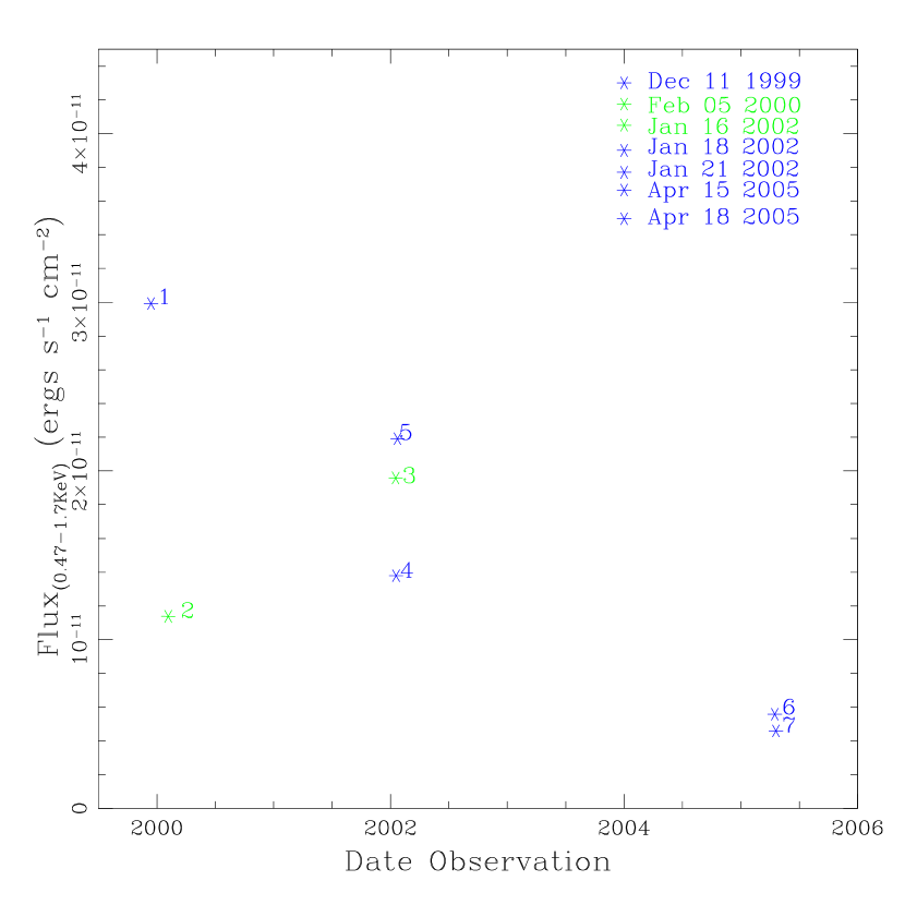
Figure 1: NGC 5548 light curve for the observations analyzed in this work. Points 2 and 3 correspond to HETGS observations and points 1, and 4-7 to LETG observations.

NGC 5548 was observed seven times with the Chandra  X-ray Observatory (Weisskopf et al. 2000) between 1999 and 2005 (see Table 1) . Two observations were carried out with the HETGS (Canizares et al. 2000) with the light dispersed on to the Advanced CCD Imaging Spectrometer (ACIS; Garmire et al. 2003). The remaining five observations were obtained with the LETGS (Brinkman et al. 2000) and the High Resolution Camara (HRC; Murray et al. 2000). We retrieved the primary and secondary data products of the observations from the Chandra data archive. The data reduction was performed with the Chandra Interactive Analysis of Observations software (CIAO v.3.4 ; Fruscione et al. 2002). We followed the data analysis threads provided by the Chandra X-ray Center. Negative and positive first order spectra were extracted and response matrices created for each observation. In this paper, we explore the time-averaged properties of the spectra, focusing on the best possible determination of the different ionization and velocity components of the well-known ionized absorber in this AGN. Thus, we co-added the spectra obtained with each instrument to get the maximum signal to noise ratio (S/N). This gave a total net exposure time of 236 ks for the MEG and HEG spectra, and 564 ks for the LEG spectrum. The source shows flux differences among observations. The change in flux between the 2 HETGS observations is $\approx$1.7. The change in flux among the LETGS data is a factor of 6 during the six years of observations (see Fig.1). The change in flux in short time scales between consecutive (LETGS) observations is $\approx$1.2-1.6 (see Table 1), (for observations separated by 3 days). A time-evolving analysis is postponed to a forthcoming paper (Andrade-Velazquez et al. in preparation). However, we discuss the possible effects that these variations in our analysis in Section 3.2.2.

We have analyzed the data in the range between (1.57 to 10.81)  Å ([1.15 to 7.90] keV) for the HEG, (2.46 to 24.58)  Å ([0.50 to 5.04] keV) for MEG, and (8.85 to 49.15)  Å ([0.25 to 1.40] keV) for LEG. All the data were binned by a factor of 2, corresponding to 0.005 Å, 0.01  Å, and 0.025  Å per bin for the HEG, MEG and LEG, respectively.

3 Modeling

We have used the CIAO software Sherpa (Freeman et al. 2001) to perform spectral fits to the data. In all the models described below, the attenuation due to the Galactic absorption was accounted for with a neutral absorber (see § 1). We first focus on the HETGS (HEG and MEG) data. Then, we compare the final HETGS model with the LETGS data, and find a good fit at both short and long wavelengths (see below).

3.1 Fitting the HETG data.

3.1.1 MODEL A: No Absorption Components.

Initially, we fit the data with a power law, following previous analysis (Reynolds et al. 1997: Advanced Satellite for Cosmology and Astrophysics -ASCA; Nicastro et al. 2000 BeppoSAX) and a black-body component (Kaastra $\&$ Barr 1989, Steenbrugge et al. 2005),see Table 2, Model A. We further added four Gaussians to model the evident emission lines (see Table 3).

Three emission lines are resolved, with FWHM between  500-700 km s^-1 (MEG has an FWHM resolution of $\backsimeq$ 155  km s^-1 at 19  Å). These lines are in the soft band (consistent with Ne ix$\lambda$13.69, O vii$\lambda$ 22.10, and N vi$\lambda$ 23.27). The short wavelength ($\leqslant 5~{}\AA$) region of the spectra shows the presence of the fourth emission line. This corresponds to the commonly found low-ionization ($\leq$ Fe xvii) Fe K_α line (6.4 keV, Nandra et al. 2007), and is located at 1.937 Å (without any shift from the rest frame of the host galaxy). Yaqoob et al. (2001) report an EW of 133 eV and a width of 4515${}^{+3525}_{-2645}~{}kms^{-1}$ and suggest a possible origin in the outer Broad Line Region (BLR). We report a full width half maximum (FWHM) of 2644$\pm$2469  km s^-1 consistent with the value reported by Yaqoob et al. We find a slightly lower EW than this authors, EW$\sim$ 92.2$\pm 43.9$ eV, however, a detailed analysis of this line is beyond the scope of this paper.

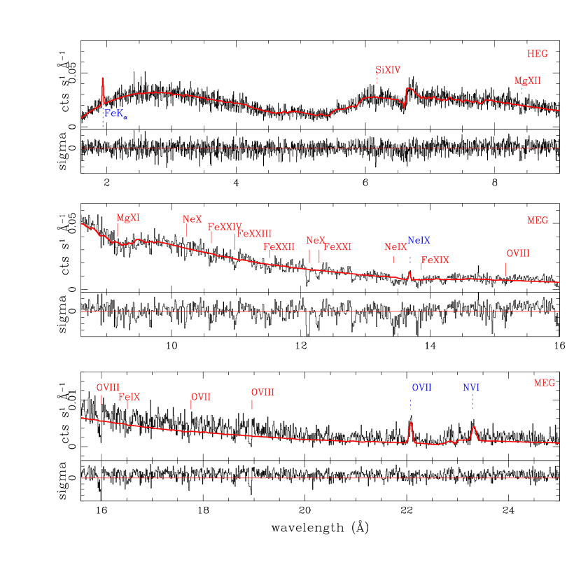
Figure 2: Model A plotted over Chandra-MEG data ( [1.6-24.5] Å) of NGC 5548. The model (red thick line) consists of a powerlaw and a black-body component plus four strong emission lines (blue labels). Possible transitions due to the ionized absorber are indicated with red labels.

Though model A was statistically acceptable ($\chi^{2}$/d.o.f.= 3813/4112), strong negative residuals between (5-24.5) Å are present, consistent with absorption features by ionized atoms (Fe xvii-xxii, O vii-viii, Ne ix-x, Si xiii-xiv, N vi-vii, and Mg xi-xii) due to the well-known WA in this source (see Fig.2).

3.2 Ionized Absorber : fitting with PHASE

To model the features produced by the ionized absorber, we used the code PHASE (Krongold et al. 2003). The code has 4 free parameters per absorbing component, namely 1) the ionization parameter at the illuminated face of the absorber $U=\frac{Q(H)}{4\pi r^{2}n_{H}c}$, where $Q(H)$ is the rate of H ionizing photons, $r$ is the distance to the source, $n_{H}$ is the hydrogen number density and $c$ is the speed of light; 2) the hydrogen equivalent column density $N_{H}$, 3) the outflow velocity of the absorbing material V_out and 4) the micro-turbulent velocity V_turb of the material. Usually, the micro-turbulent velocity is not left free to vary, because the different transitions due to ionized gas are heavily blended, or because the different velocity components are also blended and cannot be resolved (e.g. Krongold et al. 2003, 2005 for NGC 3783). In the case of NGC 5548, with the HETGS data resolution, it is possible to distinguish two velocity components (see below). So, despite the fact that the individual absorption lines cannot be resolved, we have left the micro-turbulent velocity free to vary (at least for the strongest absorbing components, see below). PHASE has the advantage of producing a self-consistent model for each absorbing component, because the code starts without any prior constraint on the column density or population fraction of any ion. We have assumed solar elemental abundances (Grevesse & Noels 1993). So, given the intrinsic Spectral Energy Distribution (SED, the approximation of this input parameter is explained in the next subsection) of the source, the column density, and the ionization parameter of the absorbing media, the ionization balance is fixed.

In all the models described below, we have assumed that the continuum source (including the soft excess) is fully covered by the ionized absorbing gas while the emission lines are produced outside the region where the absorbing material is located.

3.2.1 Spectral Energy Distribution

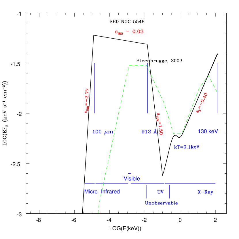
Figure 3: Spectral Energy Distribution used in this analysis (black solid line) to model the ionized absorber in the Chandra data of NGC 5548 (the SED is based on our observations and NED data, see §3 for details). Blue labels mark different observational bands (see § 3). The slopes adopted in each band are marked with red labels (this slope relates to the photon index as $\Gamma$=s+2). The dashed green line represents the SED used by Steenbrugge et al. 2005.

The X-ray to radio SED of NGC 5548, used to calculate the ionization balance of the gas, was defined in the following way: Between the radio and the near UV ranges, we used (non simultaneous) data from NED (NASA/IPAC Extragalactic Database, references are attached in Appendix §A ). In the range between 100 $\mu$m and 912 Å, we performing a linear fit to the over 100 references of flux measurements found in NED. For the region between (0.25-7.90) keV ( [1.57 - 49.15] Å), we used the power law ($\Gamma$) as well as the black-body contribution, as inferred from the fits to the continuum presented in Table 4. For energies $\geq 8$ keV, we extrapolated the derived $\Gamma$ in our fits up to 130 keV, where a cut-off is observed (Nicastro et al. 2000). Given that the UV SED shape has only a second order effect on the ionization balance of the X-ray species, as these charge states have ionization potentials larger than 0.1 keV (see Netzer 1996, Steenbrugge et al. 2003), we have connected the unobservable region of the SED between 912 Å and 0.25 keV with a simple power law (Haro-Corzo et al. 2007). The radio region (at 21 cm) was connected with the infrared (100 $\mu$m) also with a simple power law. Figure 3 shows the final SED used in this work.

3.2.2 Modelling Averaged Spectra

An important caveat of averaging the different datasets is that the the physical properties of the absorbers might have changed among observations, either because of intrinsec changes or because of changes induced by the variations in the flux level. We note, that Kaastra et al. 2002 and Steenbrugge et al. 2005 report similar values for the Hydrogen equivalent column density (within the uncertainties) for the 1999 and 2002 observations (see Table 1). Then, we do not expect a significative change in the equivalent Hydrogen column density among the seven observations. The same is true for the outflow velocity of the absorbing gas.

However, the flux level changes between the observations used in this work. Assuming the gas is in photoionization equilibrium, this would drive changes by the same factors observed in the ionization parameter (U) of the gas (producing changes in the gas opacity; Nicastro et al. 1999). There is a flux variation by a factor of 1.7 between the HETG observations, thus, the expected variation between these two observations will be Delta (logU) = 0.23. For the LETG observations, there is a large change in flux (by a factor of 6 during 6 years; see Fig. 1) between the first and last two observations. In photoionization equilibrium this would produce a change Delta(logU) =0.77 in the ionization parameter. Thus, our determination of this parameter in the co-added data will represent a weighted average over the different observations. We note that for the LETG, the 1999 and 2002 observations have the higher S/N and similar fluxes (different by a factor $\sim 2.19$, and also similar to the HETG observations). Then, the best fit value of the absorbing gas ionization parameter on the LETG co-added spectrum will be highly dominated by these observations (the inclusion of the 2005 fainter observations contribute to increase the S/N by $\sim 10\%$).

3.3 Ionized Absorber

3.3.1 Model B: One Ionized Absorber Component.

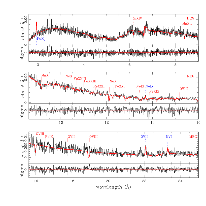
Figure 4: Model B plotted over Chandra-MEG data ( [1.6-25] Å). This model (red thick line) includes the same components of model A plus one absorbing component. Emission and absorption lines are marked as in Figure 2.

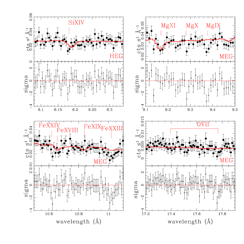
Figure 5: Model B and residuals in selected regions of the spectrum showing that the presence of additional absorbing material with higher and lower ionization is required by the data.

We made a new model, B, by including a single ionized absorbing component to model A. Table 5 shows the best fit parameters values for this model. The outflow velocity is $\sim$  -740$\pm 150$ km s^-1 and could correspond to the UV component 2, which has a value $\sim$  -667 km s^-1. Given the ionization parameter (logU_B) and column density (logN_HB) of this component (see Table 2), this model fits the absorption lines produced by ions such as Fe xvii-xxii, Ne ix-x, Si xiii, Mg xi-xii, and O viii (see Fig. 4 ). The fit gives a significant improvement over model A ($\chi^{2}=3053$ for 4108 d.o.f.; $\Delta\chi^{2}=760$). An F-test gives a higher than $99.99\%$ confidence level for the presence of the absorber (see Table 2). The absorbing component can reproduce $\sim$ 20 absorption features (including blends) in the wavelength region (5 - 20) Å. However, significant residuals remain at 6.18 Å, which are probably due to a Si xiv transition ($\lambda$6.182), and at 10.62 Å and 11.01 Å, probably corresponding to transitions by Fe xxiv($\lambda$10.619) and Fe xxiii($\lambda$11.019), see Figure 5; indicating the possible presence of another absorbing component of gas with higher ionization. Strong residuals found close to 16.5 Å, could correspond to inner transitions of Fe ix, further suggesting the possible presence of another absorber with lower ionization state.

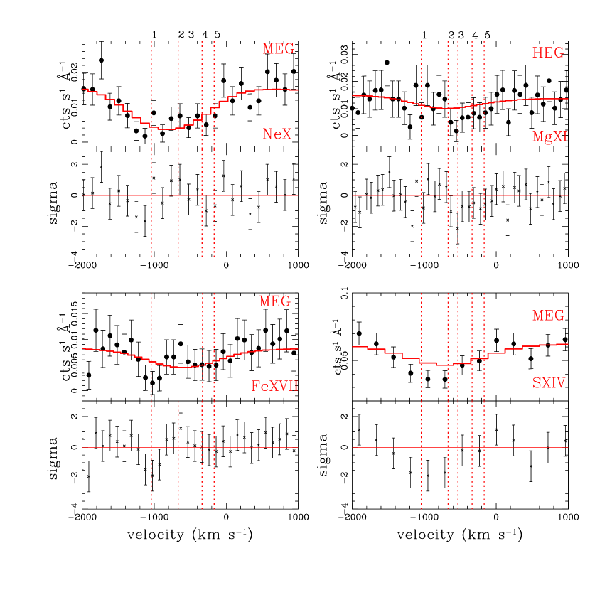
Figure 6: Detailed line profile for several absorbing features that are not well fitted by only one broad absorbing component. The dotted lines correspond to the outflow velocity of the UV components (Crenshaw et al. 2003). Significant residuals are found with outflow velocity consistent with UV component 1.

In addition, a detailed inspection of the spectrum near the absorption lines fit by this model (Mg xi, Ne ix, Fe xvii, and Si xiv) reveals a complex structure in the line profile, with additional absorption with an outflow velocity of $\sim$ -1040 km s^-1 (see Fig. 6). These results, implying additional components and complex velocity structure, are consistent with the analysis of Steenbrugge et al. (2005). We will model these additional components in the following sections.

3.3.2 Model C: Two Ionized Absorber Components.

Model C includes two absorbing components, whose parameters are again free to vary. This model gives a $\chi^{2}=2987$ for 4104 d.o.f., significantly improving over model B ($\Delta\chi^{2}=66$, an F-test, gives a confidence of larger than $99.99\%$ for the addition of these parameters). The ionization parameters (logU_C1 and logU_C2) are different by almost a factor of 3 (see Table 5).

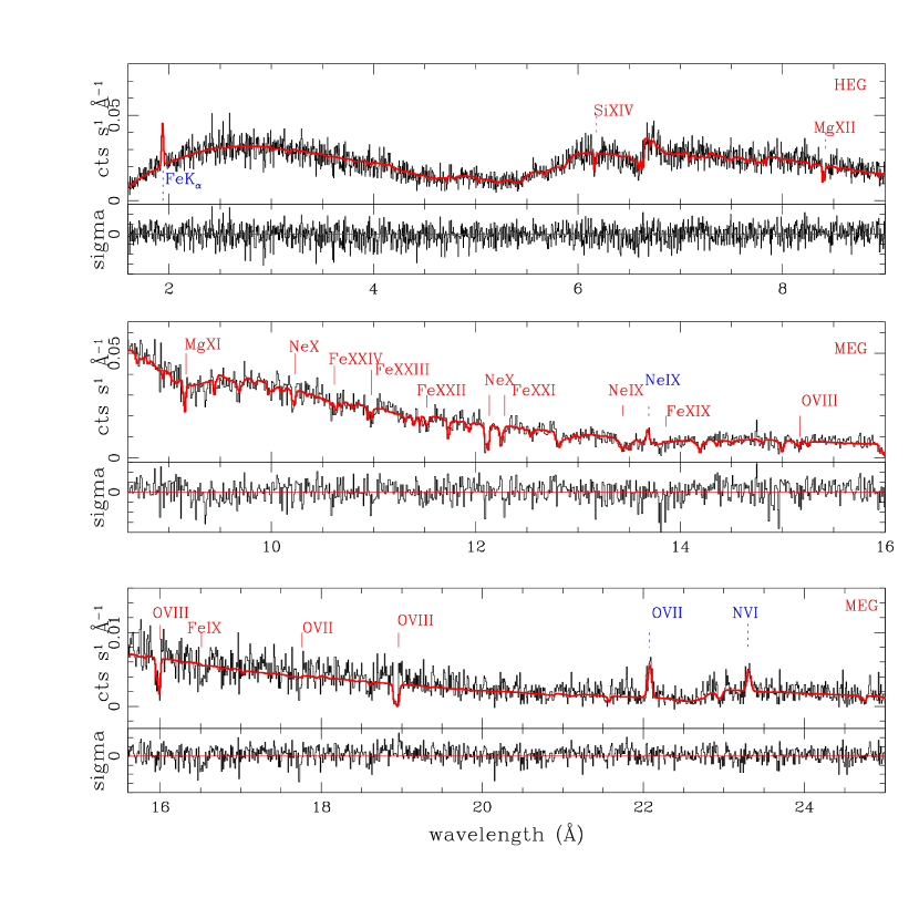
Figure 7: As Figure 4, but for model C, which includes two absorbing components. This model can fit transitions by both high and medium ionization level ions such as Fe_XXIII-XXIV.

The component with lower ionization (with logU_C2 slightly lower than logU_B1) models the transitions already fitted in model B: Si xiii-xiv, Ne ix-x, Mg xi-xii, Fe xvii-xxii, and O viii  (see Fig. 7). The higher ionization component (with logU${}_{C1}\sim 1.4\times$logU_B1) contributes weakly to fit these ions, but fits the transitions due to Fe xxiii-xxiv (not fitted in model B). The two components have different outflow velocities ( V_outC1 = -1120 km s^-1 and V_outC2 = -450 km s^-1) . We note that while model B partially fits the Si xiv  line, the higher ionization component in model C (logU_C1), which has also higher outflow velocity, improves the fit to the Si xiv line, i. e. this component fits the residuals that model B left around 6.18 Å  (see Fig. 7). While model C does reproduce, then, the lines produced by Si xiv , Fe xxi-xxiv, it cannot model the complex absorption profile observed also for other lines.

3.3.3 Model D: Three Ionized Absorber Components.

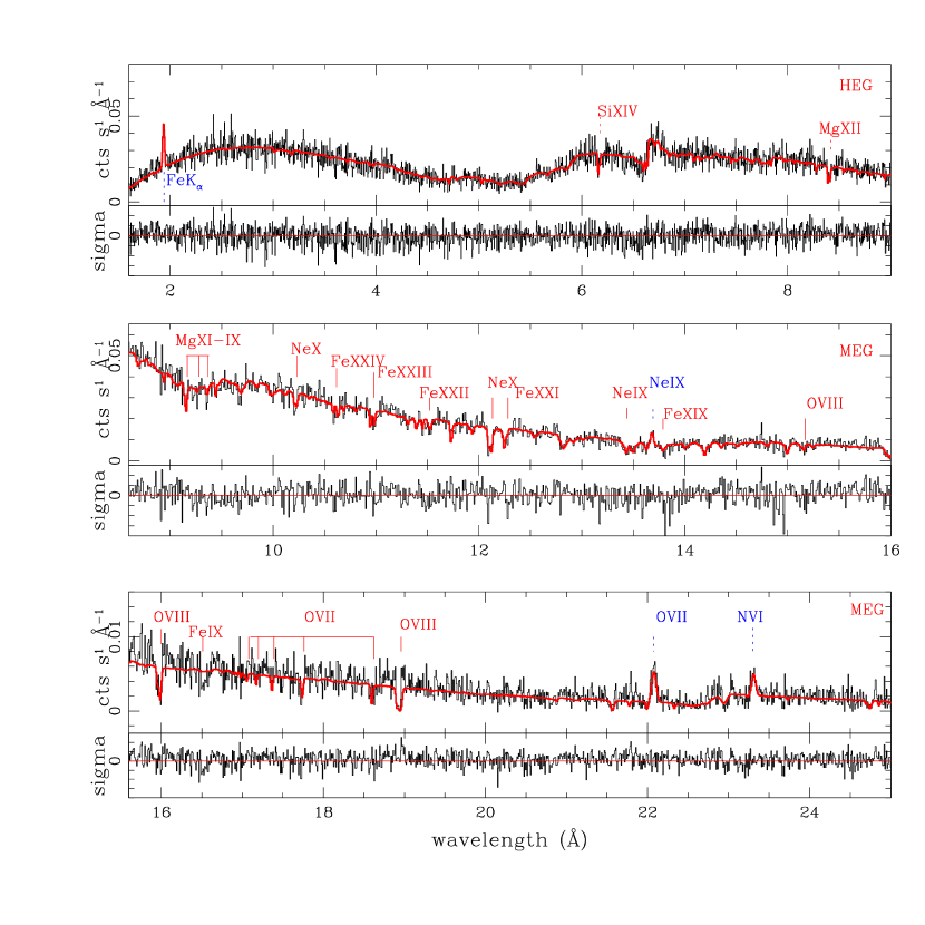
Figure 8: As Figure 4, but for model D (red thick line), which includes three absorbing components. The contribution of the lower ionization component is observed in transitions such as Mg_IX-XI and O_VII.

Motivated by the line profile residuals, we built a new model, D, by adding a third absorbing component, whose parameters are again free to vary, as are those of the other two components. Model D gives a $\chi^{2}=2946$ for 4100 d.o.f., improving significantly model C ($\Delta\chi^{2}=41$, F-test confidence level of $99.99\%$). All the three absorbing components have different ionization level. Two of the three absorbing components have similar values of logU to those found in model C. The third component has a much lower ionization level (by at least a factor $\sim 14$, see Table 5), and fits the N vi-vii, O vii, Mg ix-xi  lines, as well as the Fe vii-xii  M-shell Unresolved Transitions Array [UTA] (see Fig. 8). The three absorbing components group in two different outflow velocity systems. One system, with outflow velocity in the range between -450$\pm 150$ and -590 $\pm 150$ km s^-1, contains the systems with intermediate ( logU_D2) and low (logU_D3) ionization level. The other velocity system (V_out = -1116 $\pm$ 150 km s^-1) is formed by the high ionization component.

We note that model D still leaves some residuals around 16.5 Å, where an Fe ix transition lies. The reason for this discrepancy may be due to our use of the abbreviated data to model the UTA (see Krongold et al. 2003 and Behar et. al 2001 for further details).

3.3.4 Model E: Four Ionized Absorber Components.

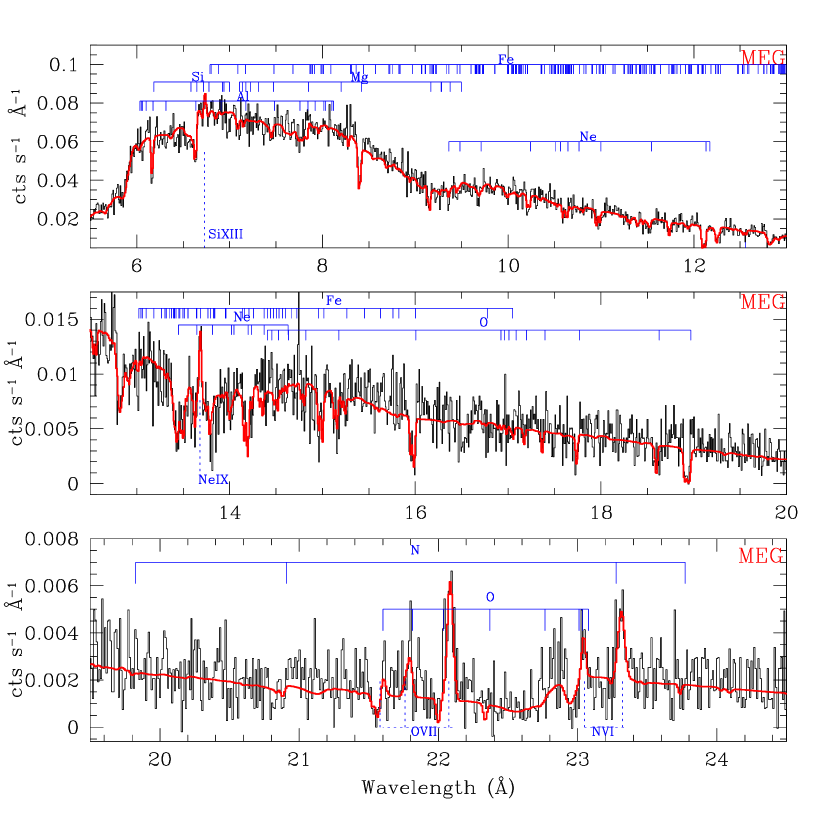
Figure 9: Model F (red thick line; corresponding to model E plus 4 additional emission lines, see § 3.4 ) plotted over the MEG spectra ([5-24.5] Å) of NGC 5548. Two velocity components, each formed by two phases, are required to fit the data. The upper labels correspond to the absorption lines, while the lower labels mark the emission features.

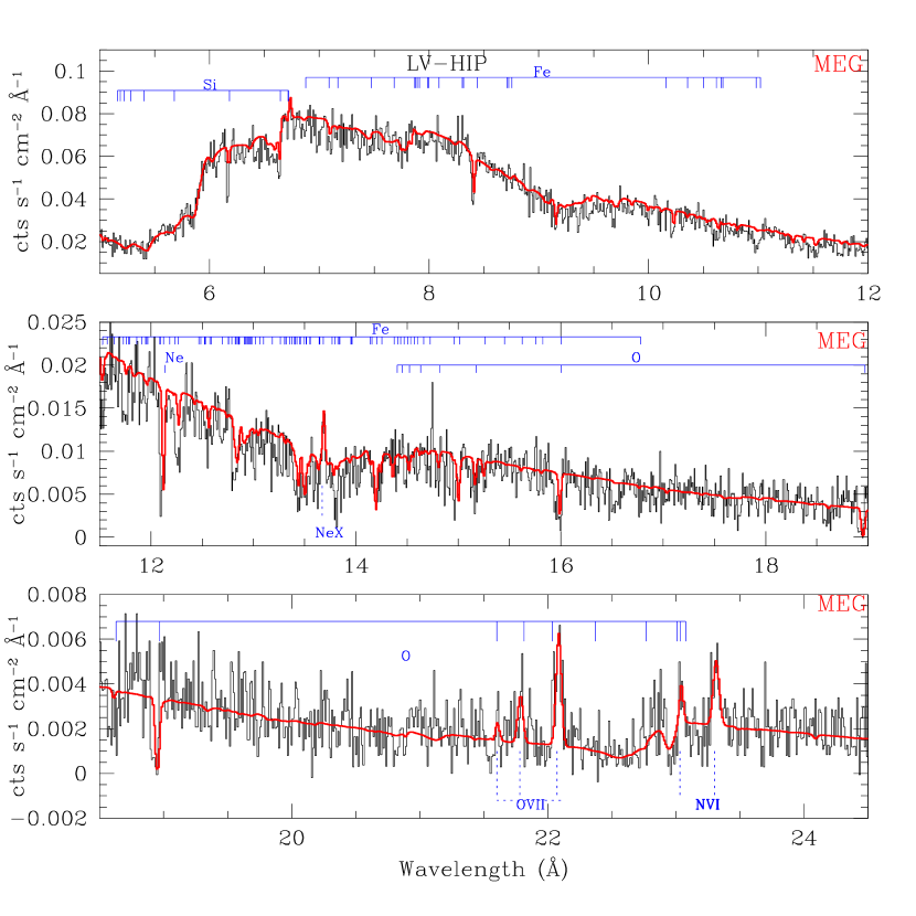
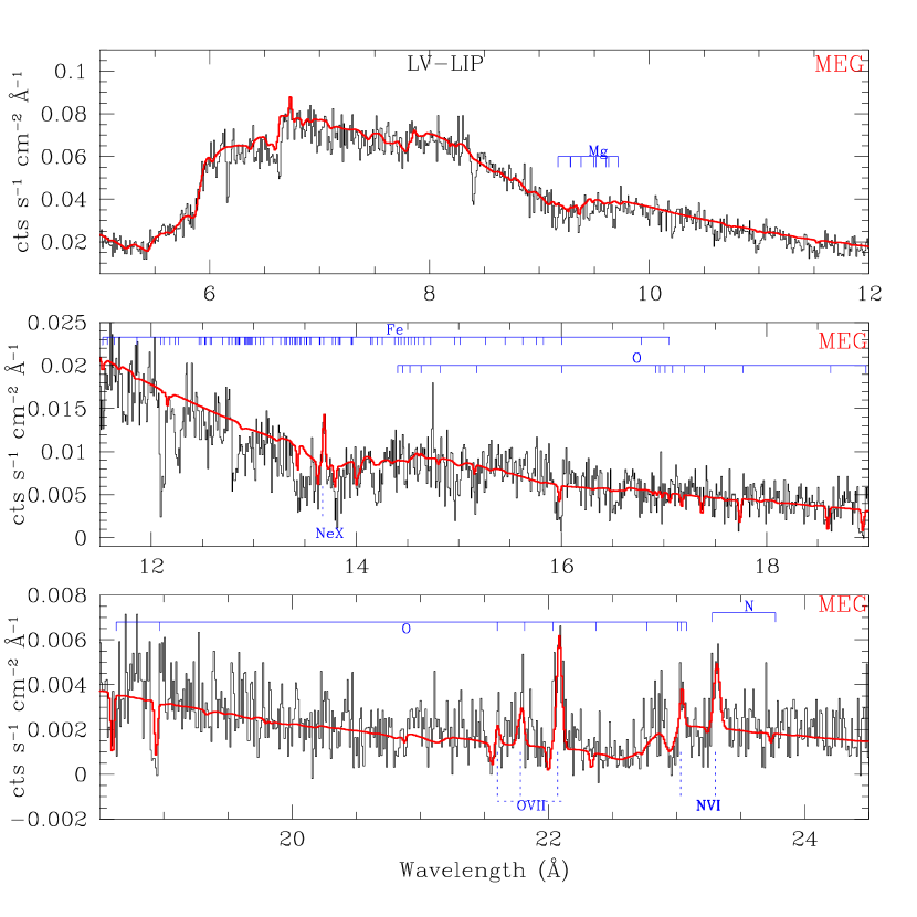
Figure 11: MEG spectrum and model between (5 and 24.5) Å showing only the contribution of the low outflow system. The left panel shows the contribution by the Higher Ionization Phase (HIP) and the right panel shows the Low Ionization Phase (LIP).

Model D does not solve the problem of the line profile for several absorption lines with intermediate ionization state, in particular the Fe xvii and Ne x  transitions. Therefore, model E was built by adding a fourth absorbing component to model D. This case gives a $\chi^{2}=2904$ for 4096 d.o.f. ($\Delta\chi^{2}=42$), which is statistically better than that of model D (an F-test shows that the fourth absorber is required at the $99.99\%$ confidence level). The best-fit parameters value for each absorbing component are listed in Table 6, and the global fit to the HETGS data is shown in Figures 9 (for MEG data) and 10 (for HEG data) . Model E again consists of two outflow velocity systems (hereafter High Velocity or HV for the system with V_out = -1110 $\pm$ 150 km s^-1, and Low Velocity or LV with V_out = -490 $\pm$ 150 km s^-1 ), each having two different ionization components. The ionization parameter of the high ionization phase in the LV system (hereafter LV-HIP) is logU=0.67 with a column density of log$N_{H}$= 21.25. The low ionization phase (LV-LIP) has log$N_{H}$= 20.74 and logU=-0.49. The features fitted by this system are the same ones fitted in model D by the components similar to that model. The contribution of this velocity component to the global fit is shown in Figure 11.

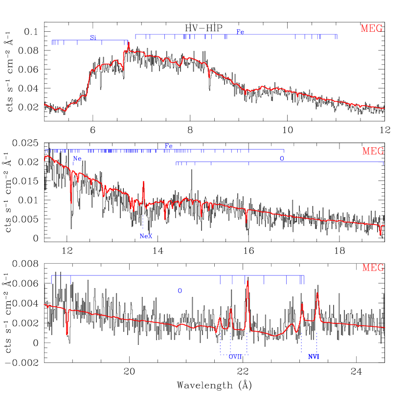
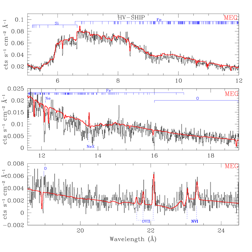
Figure 12: MEG spectrum and model between (5-24.5) Å showing only the contribution of the HV-HIP, and the right panel the HV-SHIP.

The HV system has two absorbing components. One of the absorbing components of this system has a high ionization level (logU=0.671, hereafter called HV-HIP), and a column density of logN_H=21.03, and the other absorber has an even higher ionization level (hereafter called HV super-high ionization phase or HV-SHIP) with logU=1.23 and logN_H=21.73. Figure 12 shows the contribution of the HV system to the global fit of the spectrum. The HV-SHIP fits the same features model D does.

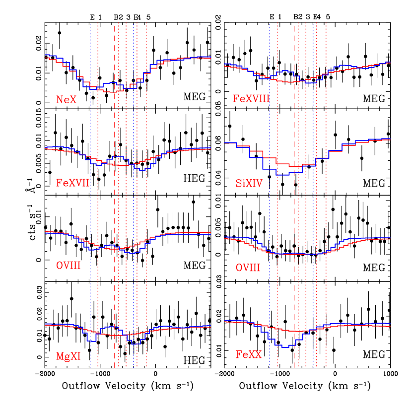
Figure 13: Model F (blue thick line) plotted against selected HEG and MEG spectral regions, showing the best fit lines profiles. The two outflow velocity systems are marked with letter E at the top of the panels, and correspond to -1180 and -400 km s^-1. The fit with a single broad profile (model B, red thick line) is also shown. The corresponding velocity of this model (-740 km s^-1) is marked with the letter B and a dashed vertical red line. The UV velocity systems (Crenshaw et al. 2003) are marked with dotted lines.

The HV-HIP of this system fits the same absorption lines as the LV-HIP (given that the ionization parameters of these two components are quite similar). The difference between these two components lies mainly in their outflow velocities, finally improving the fit to the line profile (as seen in Fig. 13). We note that this result is obtained without any constraint in the main parameters of the absorbers, which further confirms the presence of the two velocity systems. Separating the two components was possible given the excellent resolution of the HETGS, $\approx$155 km s^-1 (19 Å) for MEG.

3.4 Emission Features in the Spectra of NGC 5548

In the previous models we fitted four strong emission lines (the Fe K_α line, and the Ne ix, O vii, and N vi  forbidden transitions). However, in the MEG data, there are four additional emission lines that can be detected with a significance level $>2\sigma$ once the absorbers are properly modelled. These lines correspond to the resonant and intercombination transitions of O vii, the resonant transition of N vi and Si xiii line. We produced a new model including these lines (model F). The best fit parameters for the eight absorption lines included to fit the HETG data are given in Table 3. Figure 9 already includes these features.

Our analysis does not require the inclusion of broad emission features (as was reported by Steenbrugge et al. 2005). The forbidden (z), resonant (w), and intercombination (x+y) lines of He-like ions (Gabriel & Jordan 1969) can be used to derive the physical conditions of photoionized plasma (Porquet $\&$ Dubau 2000). In particular, the ratio between the resonant and intercombination lines serve as a diagnostic of the electronic density n_e (R(n_e) = $\frac{z}{x+y}$). Using the R value of the O vii lines (R(n_e)= 2.23$\pm 1.6$), and following Porquet $\&$ Dubau (their Figure 8), we find that the gas must be photoionized and must have a density n${}_{e}=2.0\pm 0.8\times 10^{10}cm^{-3}$. Kaastra et al. (2000) report an upper limit for n${}_{e}<$ 7.0$\times 10^{10}cm^{-3}$, with a R(n_e) = 2.22$\pm 3.45$, which is in agreement with our result.

3.5 Extrapolation to LETGS

The final model (F) for the ionized absorber in the MEG and HEG spectra of NGC 5548 can be further tested by extrapolating to the LETGS data (the LETGS resolution is a factor $\sim$ 2.5 worse than the MEG resolution at 19 Å). In doing this, we implicitly assume no significant opacity variations between the co-added HETGS and LETGS spectra that may arise from flux variability (Nicastro et al. 1999, Krongold et al. 2005b, 2007). Given that the average flux level in these two spectra differs by only 30% (Steenbrugge et al. 2005), this is a reasonable assumption .

To fit the LEG spectrum, we used model F, with the 4 absorbing components’ parameters fixed to the values obtained for the HETGS data (hereafter model G). We also used the same continuum components (a power law and a black-body), but we allow these parameters to vary freely in the fit, as the continuum level and spectral shape might be different (in addition, the LETGS is more sensitive to low energy photons and so these data allows for a better determination of the black-body temperature). In model G we also let free to vary the parameters for the emission lines detected in the HETGs spectra (except for the Fe k$\alpha$ and Si xiii lines that lie outside the spectral range of the LETG). We further added three additional emission lines, (located in wavelengths larger than 25 Å, the lower bound of the MEG data), corresponding to Nv$\lambda 29.502$, N vi$\lambda 29.029$, and C v$\lambda 41.429$).

An acceptable fit is obtained to the LETGS spectrum with this simple method ($\chi^{2}/d.o.f.=2013/1618$), implying that the HETGS spectra alone can constrain in a reliable way the properties of the ionized absorber. The best-fit continuum parameters for the LETGS spectrum are collated in Table 4. Table 3 presents the parameters for the emission lines.

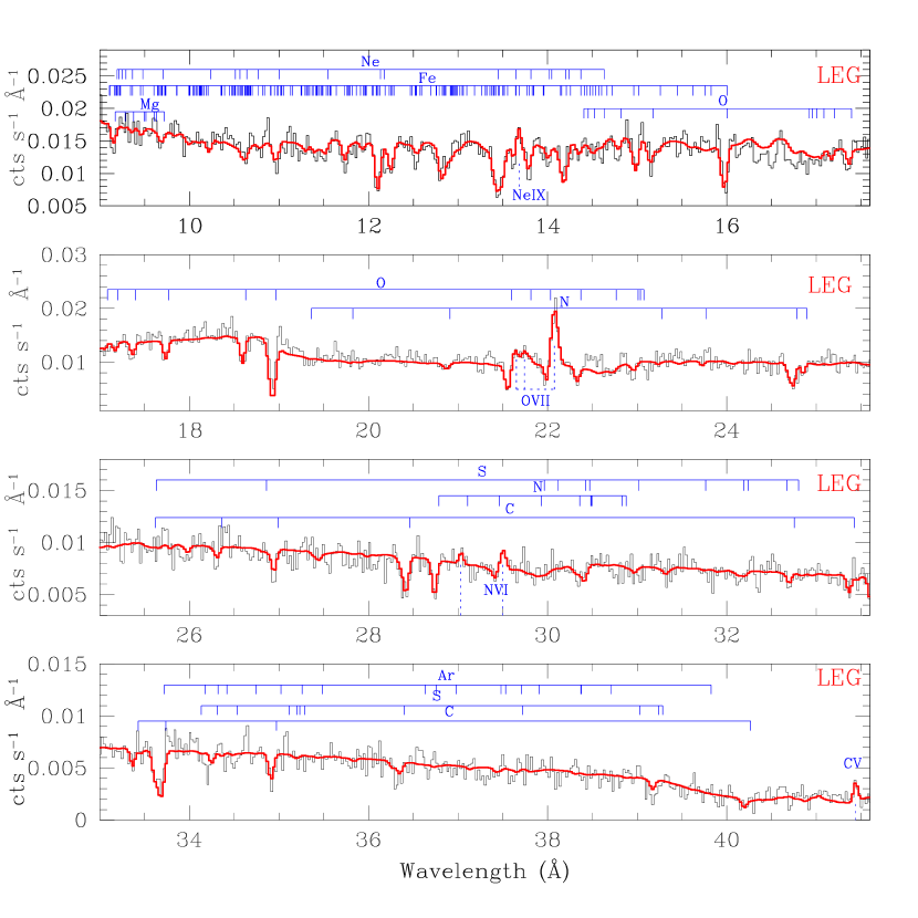
Figure 14: The best fit for WA on the HETGS data extrapolated to the LETG data (model G). This model shows a good fit on the LEG spectral region ( [9-41.6] Å). The O_VII, N_VI, Ne_IX and C_V emission lines are marked with dotted blue lines.

The best-fit model over the data is presented in Figure 14 (see also Table 2). This figure show that most absorption lines observed in the HETG data are well reproduced by the model in the LETGS spectrum. It also shows that model G fits well more than 12 low ionization absorption lines in the region (26-49) Å. These lines correspond to transitions of ions such as C v, N v-vi, and S xii. In the UTA region there are discrepancies between data and model, but as for the HETGS data, they are produced likely due to the use of the abbreviated data to model this feature.

We note that some low ionization lines show residuals consistent with an outflow velocity of -1040 km s^-1 as shown in the Figure 15. This may indicate the presence of a HV-LIP (see §4). However, attempting to model these residuals with an additional absorbing component does not improve the fit in a statistical way.

4 Discussion

The best fit model of the WA for the Seyfert 1 galaxy NGC 5548 requires two outflow velocity systems, each with two different ionization phases (§3). Figure 13 shows that the profiles of the absorption lines (produced by ions such as Ne x, Fe xviii, O viii, and Mg xi) are fit better with two narrow line profiles than with a single broad component. Each of these two velocity components requires absorption by gas with very different ionization level. The LV component consists of gas with two different ionization states (the LV-LIP and the LV-HIP). The HV component requires also two absorbers with different ionization (the HV-SHIP and the HV-HIP). These four absorbers, divided into two velocity systems, can reproduce all the spectral features observed in the spectra (Fe vii-xxiv, O vi-viii, Ne ix-x, Mg ix-xii, Si xii-xiv, C v-vi, S ix-xii, and Ar xi-xii). We note that the HV system might also have an additional, low ionization component (HV-LIP). Figure 15 shows a double line profile for several low ionization level lines, suggesting a LIP with higher outflow velocity (-1041 km s^-1). While the inclusion of this component is not statistically required by the data, its physical properties appear to be well constrained (as can be observed in in Figure 16, where the 1, 2, and 3$\sigma$ confidence regions for the ionization parameter vs. the column density of this component are presented). Further evidence for the presence of this component arises from the fact that UV system 1 can be associated with the HV absorber (see §4.1), and the HV-SHIP and HV-HIP have a very hgh ionization state to produce such absorption ((see Tables 7 and 8). We conclude that the data clearly shows a shift to higher ionization material at higher velocity in NGC 5548 WA, with the LIP becoming weak and the SHIP dominating in the HV system. On the other hand, the LV system does not show the presence of the SHIP.

The separation between components is a new and important feature in X-ray spectra of ionized absorbers, and could be achieved because of the large difference in velocity between the two systems ($\sim 500-600$ km s^-1), as well as the different dominant ionization levels between them (see also Steenbrugge et al. 2005).

4.1 UV Counterparts

In the study of the narrow Ovi, Nv, and Civ absorption lines in the UV region, Crenshaw et al. (2003) finds five separate kinematic components in $\it HST$ -STIS and $\it FUSE$ spectra. Our analysis reports two kinematic components (HV and LV systems). The HV system shows similar outflow velocity to the UV absorbing component 1 ($-1041$ km s^-1). According to Crenshaw et al. (2003)b, the gas producing absorbing component 1 should produce only a weak X-ray WA, which is consistent with the marginal detection of the HV-LIP in the Chandra data (§ 4).

There is also a correspondence between the X-ray LV system and UV absorbing components 2 and 3 (with outflow velocities $-667$ and $-530$ km s^-1, respectively). Crenshaw et al. (2003)b and Crenshaw et al. 2009 suggest that at least component 3 (and possibly component 2) should produce absorption in the X-ray range. This is consistent with the detection of the LV-LIP. There is no X-ray detection of UV absorbing systems 4 and 5 (with velocities $-336$ and $-166$ km s^-1 respectively), although we cannot rule out a possible contribution from component 4 to the LV-LIP, given the uncertainty in the outflow velocity of the X-ray systems. According to the analysis of the UV data by Crenshaw et al., system 5 has the lowest column density (logN_H=19.27). Krongold et al. (2003) discuss how the difference in sensitivity of the current X-ray and UV detectors may affect the detection or non-detection of a given UV component in the X-rays. Their Figure 11 shows the observational lower limits for the equivalent widths of the Civ$\lambda\lambda 1548.2,1551$, Ovi$\lambda\lambda 1038,1032$, O vii$\lambda 21.602$, O viii$\lambda 18.968$ lines detectable in the UV and X-ray bands, as a function of the ionization parameter and H equivalent column density. Thus, given their ionization state and column density, systems 4 and 5 are consistent with not being detected in the X-rays, given the limited sensitivity of the X-ray observations.

While a kinematic connection between the components is evident, an important question is how the predicted/measured column densities for the different analyses compare between them. The ionic column densities predicted by our model are now listed in Table 7 and 8 for the LV and HV systems, respectively. In these Tables, we also list the column densities predicted (or measured) by Crenshaw et al. (2009), based on UV data, and by Steenbrugge et al. (2005), based on the LETG 2002 data (their model B, see §4.3). The column densities for ions CIV, NV y OVI between our predicted values and those measured by Crenshaw et al. (2009) in the UV differ by factors of   16, 4 and 1.2, respectively. We note that OVI (where no diference is found) is detected in the X-ray analysis as well. The differences between the UV and X-ray columns could be produced because of 3 different factors: 1) The blending of UV components 2 and 3 in the X-rays (and maybe an additional contribution from UV component in our LV-LIP model. 2) The different SEDs used in the 2 analysis: The SED used by Crenshaw et al. includes much more photons in the far (unobservable) UV, and 3) A detailed analysis on the dependence of the covering factor on velocity could not be performed in the analysis of the UV line profile. This could underestimate the columns as shown by Arav et al. 2003. Taking into account these effects, we consider that the predictions of our model for the columns measured in the UV are very reasonable, and conclude that the LV-LIP component can produce the absorption features produced by UV component 3 (and maybe 2 and 4). However, we note that the values predicted by Crenshaw et al. for the high ionization charge states differ from those measured in this analysis. The reason for this discrepancy, is that these ions are not observable in the UV, and only three ions (CIV, NV y OVI) were used in the UV model.

With these considerations, and given the strong coincidence in kinematics between the UV and X-ray outflows, we conclude that a common origin is not only possible, but quite likely. Such connection was originally suggested by Mathur et al. (1994) for NGC 5548, and has also been suggested for several other objects (NGC 985- Krongold et al. 2005; NGC 3783-Gabel et al. 2003, Krongold et al. 2003, Netzer et al. 2003; NGC 7469- Blustin et al. 2003, Kriss et al. 2003). Thus, these studies on the WA may represent a general feature of the structure for quasars, as proposed by Elvis (2000).

4.2 Two Multi-phase Absorbing Outflows

The presence of two different absorbing components with different temperature but similar outflow velocity suggests that the absorber may be formed by a multi-phase medium (e.g. Elvis, 2000; Krongold et al. 2003). Given the two velocity systems in NGC 5548, we could be seeing the presence of two different outflows (with different outflow velocity), each being a multi-phase medium.

This is further supported by the pressure equilibrium of the two absorption components in each velocity system. In Figure 17 we show the thermal stability curve of the gas (also known as the ”S-curve”, Krolik et al. 1981) for the SED used in our analysis (§3.2.1; Fig. 3). The S-curve marks the points of thermal equilibrium in the T vs. U/T plane, where T is the photoionization equilibrium temperature of the gas, and U/T is inversely proportional to the gas pressure (U/T $\propto P_{rad}/P_{gas}$ ).

In Figure 17a, the position on the S-curve of the two LV absorbing components is shown. The LV-HIP and the LV-LIP have quite different temperatures but, within the errors, are consistent with a single value of the U/T, and so can be in pressure equilibrium. Figure 17b shows the HV-SHIP and HV-HIP on the S-curve. Again, the pressure equilibrium between the two components is allowed. Note that, given the possible range of ionization parameters of the tentative HV-LIP (Figure 16), this component, if indeed present (as suggested by our results and by those by Crenshaw et al. 2009), could also be in pressure equilibrium with the higher ionization ones that form this system. Thus, both the HV and the LV systems are formed by a two-phase medium (or maybe three-phase for the HV system), with one component pressure confining the others (see Krongold et al. 2005a for a more detailed explanation).

NGC 5548 thus joins the group of AGNs for which pressure equilibrium applies: NGC 3783 (Krongold et al. 2003, Netzer et al. 2003), NGC 985 (Krongold et al. 2005, 2008), NGC 4051 (Krongold et al. 2007), Mrk 279 (Fields et al. 2007), UGC 11763 (Cardaci et al. 2009). No other well studied WA in a Seyfert galaxy is inconsistent with the description of a multi-phase medium. We note however, that we will further test this idea for the WA over a large sample of objects (Andrade-Velazquez et al. in preparation). NGC 5548 is the first AGN in which a two-phase WA medium is likely for two velocity systems. The presence of a multi-phase medium obviously requires that the different ionization components that form it lie at the same distance from the ionizing continuum. We do not have the means to test this requirement (though see Krongold et al. 2010). However, for NGC 4051, Krongold et al. (2007) measure the distance of the two absorbing components and found that they were indeed consistent with being co-located, giving further plausibility to multi-phase absorbing winds.

The SHIP of the HV system and the HIP of both the LV and HV systems lie on unstable regions of the S-curve, implying a possible inconsistency with the multi-phase scenario. However, the shape of this curve depends on the exact shape of the SED of the source, which has major uncertainties, particularly in the extreme UV region (Haro-Corzo et al. 2007). The chemical composition of the absorbing gas has an important effect on this curve also (see Komossa & Mathur, 2001, Fields et al. 2007). In addition, recent studies of the S-curve with new and more reliable dielectronic recombination rate coefficients (Badnell et al. 2006) show that there is a larger probability of having a thermally stable WA at 10⁵ K, (Crenshaw et al. (2009) obtain a T $\sim$ 1$\times 10^{5}$ for the UV component 3), and then a greater plausibility for its multiphase nature (Chakravorty et al. 2008).

4.3 Comparison with Previous Works

Steenbrugge et al. (2005) analyzed three Chandra grating observations of NGC 5548 (those carried out on 2002, Table 1) with a total exposure time of 494 ks. They presented a model showing that a continuous distribution of column densities and ionization parameters could fit the data. They further concluded that the data was not consistent with discrete phases of material in pressure equilibrium.

This conclusion is in contradiction to the results presented here, making a detailed comparison of both analysis necessary. In their model C, Steenbrugge et al. (2005) explored a model similar to the one presented here. They used a self-consistent model that takes advantage of photoionization balance calculations to make a global fit to the data. They concluded that following this approach, and fitting Fe separately, a good fit could be obtained, but constraining only two absorbing components. They further tested the presence of discrete components by adjusting equivalent H column densities and ionization parameters to the absorbing components of their model B, where ionic column densities were measured on an ion by ion fit. In this case they find that at least five different components with different ionization state were required. This approach led them to conclude that discrete components were not a good representation of the data.

The most fundamental difference between the analysis carried out by Steenbrugge et al. (2005) and the present analysis is that their models B and C used only a single velocity outflow with a large turbulent broadening to fit the data. However, as they report in their paper, and as discussed here, the data are better fitted with two different velocity components, the HV system and the LV system. Furthermore, as shown here (and as also noted by Steenbrugge et al.) the degree of ionization is different for the different velocity components, as the HV system becomes dominant for high ionization states. This led them to conclude that more and more ionization components were required to fit the data and thus a structure of discrete clumps of gas was unlikely. However, here we have shown that, when each velocity component is modelled independently, both can be well described by two ionization components, making the presence of discrete components plausible and likely. Furthermore, the addition of extra components does not improve the fit. So, given the difference between number of free parameters from the different models, we can claim by Occam’s razor that our global approach is preferable. Table 7 and 8 show the column densities for our model and the Steenbrugge et al. model B. The differences found between our analysis and that by Steenbrugge et al. (that analysis shows sistematically larger columns than ours) are likely produced because only one velocity component was used by Steenbrugge et al. to model the line profile produced by the two velocity systems. A detailed fitting including the line profile of each velocity system produces more reliable column densities.

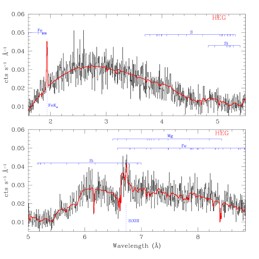
Figure 10: Model F (red thick line) plotted over the HEG spectra ([1.6-8.84] Å) of NGC 5548.

Steenbrugge et al. (2005) further tested whether their five discrete components could be in pressure balance, and they concluded that they could not. In fact, their S-curve (their Fig.10) has no region where the slope is negative, making it impossible for the gas to be in pressure balance. We stress again that the shape of the S-curve depends strongly on the metallicity of the absorbing gas, and the shape of the SED used to produce it (in this work we use the best multiwavelength data available extracted from NED). Given this, and the new results by Chakravorty et al. (2008), we conclude that the possibility that the different phase are in pressure equilibrium cannot be discarded. Here we have shown that when the velocity systems are modelled independently, each one is consistent with pressure balance. We further note that Chelouche (2008) also find that the WA in NGC 5548 can be described by a multiphase medium. The author models the ionized flow assuming a thermal wind. While his model is more physically driven than ours, it does not take into account the two different velocity systems revealed by the data. However, given the similar results, the idea of a multi-phase medium absorber is reinforced.

4.4 Possible Geometry of the Ionized Outflow

The presence of two different velocity systems, each formed by gas with very different ionization state, can give a clue about the structure of the flow. In a continuous radial range of ionization structures, the wind must extend in our line of sight for parsecs (or more), forming a large scale outflow along our line of sight. We find difficult to reconcile such a distribution of material with the two velocity systems found in NGC 5548, even if inhomogeneities in the flow (like those suggested by Ramírez et al. 2005) are invoked. The presence of the two velocity components, then, suggests that we are not seeing the wind in a radial direction.

On the other hand, the presence of the different kinematic components can be naturally explained if we are looking at an outflow in a transverse direction, which is consistent with the detection of transverse motion in the UV absorbers (Marthur et al. 1995, Arav et al. 2002, Crenshaw et al. 2003). In this case, an important component of the velocity (and acceleration) of the wind could take place in the direction perpendicular to our line of sight. Such a configuration for the wind is further supported by the finding that the different phases observed at each velocity form a single multi-phase outflow.

If the wind arises from the inner accretion disk (Konigl & Kartje, 1994, Elvis et al. 2000, and Krongold et al 2007), and flows in a transverse direction with respect to our line of sight, the two velocity components could be simply explained as forming in different regions of the disk (Elvis, 2000). The two velocity components in NGC 5548 are consistent with originate in the accretion disk, as discussed by Krongold et al. (2010). Furthermore, Crenshaw et al. (2009) suggest that UV component 3 (clearly associated to the LV-LIP), should be accelarated by magnetocentrifugal forces, and thus should form at an accretion-disk scale (Bottorff et al. 2000). We note that an accretion-disk wind does not imply a small scale outflow. The wind could still extend for large scales, but our line of sight would cross it only at a given distance from the central ionizing source.

5 Conclusions

We find that the WA of NGC 5548 can be modelled in a simple way with two different velocity systems (V_out = -1110 km s^-1 and V${}_{out}=-490\pm 49$ km s^-1) each with two phases of gas in pressure equilibrium. This results strongly suggests that the structure of the absorber in NGC 5548 could consist of two different outflows (with different outflow velocity), each formed by a multi-phase medium in pressure balance. The ionized absorber in NGC 5548 now fits a pattern established for the other well studied systems. There are no remaining cases in which a multi-phase medium is inconsistent with the observations.

The presence of two velocity systems, each formed by a multi-phase medium suggests that we are looking at the flows in a transverse direction with respect to our line of sight (as also suggested by the UV data).

The velocity of the two X-ray absorbing systems is in agreement with components 1, 2, and 3 found in the UV band (Crenshaw et al. 2003b). The X-ray data are further consistent with the non detection of UV components 4 and 5, given the limited sensitivity and resolution of the current X-ray (compared to those in the UV). There is also a reasonable agreement in the column densities of CIV, NV, and OVI predicted by our X-ray analysis, and those measured in the UV. Thus, our models elegantly solve the long-standing problem of apparent discrepancies between the UV and X-ray absorbers, and give further support to the idea that UV and X-ray absorbers are part of the same outflow.

Appendix A APPENDIX

In this appendix we have enumerated (from high to low energy) the 31 references for the 185 photometric data points from NED used to build the Spectral Energy Distribution.

1. Kaspi, Shai; Maoz, Dan; Netzer, Hagai; Peterson, Bradley M.; Vestergaard, Marianne; Jannuzi, Buell T.  2005, ApJ, 629, 61K

2. McKernan, B.; Yaqoob, T.; Reynolds, C. S.  2007, MNRAS, 379, 1359M

3. Jack W. Sulentic, Rumen Bachev, Paola Marziani, C. Alenka Negrete, and Deborah Dultzin  2007, ApJ, 666, 757S

4. Muñoz Marín, Víctor M.; González Delgado, Rosa M.; Schmitt, Henrique R.; Cid Fernandes, Roberto; Pérez, Enrique; Storchi-Bergmann, Thaisa; Heckman, Tim; Leitherer, Claus  2007, AJ, 134, 648M

5. Anderson, Kurt S.  1970, ApJ, 162, 743A

6. McAlary, C. W.; McLaren, R. A.; McGonegal, R. J.; Maza, J.  1983, ApJS, 52, 341M

7. de Vaucouleurs, G.; de Vaucouleurs, A.; Corwin, H. G., Jr.; Buta, R. J.; Paturel, G.; Fouque, P.  1991, RC3.9, C.

8. Koulouridis, E.; Plionis, M.; Chavushyan, V.; Dultzin-Hacyan, D.; Krongold, Y.; Goudis, C.  2006, ApJ, 639, 37K

9. Suganuma, Masahiro; Yoshii, Yuzuru; Kobayashi, Yukiyasu; Minezaki, Takeo; Enya, Keigo; Tomita, Hiroyuki; Aoki, Tsutomu; Koshida, Shintaro; Peterson, Bruce A.  2006, ApJ, 639, 46S

10. Zwicky, Fritz; Herzog, E.  1963, CGCG2.C…0000Z

11. Takamiya, M.; Kron, R. G.; Kron, G. E.  1995, AJ, 110, 1083T

12. Petrosian, Artashes; McLean, Brian; Allen, Ronald J.; MacKenty, John W.  2007, ApJS, 170, 33P

13. Bentz, Misty C.; Denney, Kelly D.; Cackett, Edward M.; Dietrich, Matthias; Fogel, Jeffrey K. J.; Ghosh, Himel; Horne, Keith D.; Kuehn, Charles; Minezaki, Takeo; Onken, Christopher A.; Peterson, Bradley M.; Pogge, Richard W.; Pronik, Vladimir I.; Richstone, Douglas O.; Sergeev, Sergey G.; Vestergaard, Marianne; Walker, Matthew G.; Yoshii, Yuzuru  2007, ApJ, 662, 205B

14. Bentz, Misty C.; Peterson, Bradley M.; Pogge, Richard W.; Vestergaard, Marianne; Onken, Christopher A.  2006, ApJ, 644, 133B

15. Lebofsky, M. J.; Rieke, G. H.  1980, Natur, 284, 410L

16. Wisniewski, W. Z.; Kleinmann, D. E.  1968, AJ, 73, 866W

17. Spinoglio, Luigi; Malkan, Matthew A.; Rush, Brian; Carrasco, Luis; Recillas-Cruz, Elsa  1995, ApJ, 453, 616S

18. Balzano, V. A.; Weedman, D. W.  1981, ApJ243, 756B

19. McAlary, C. W.; McLaren, R. A.; Crabtree, D. R.  1979, ApJ, 234, 471M

20. Rieke, G. H.  1978, ApJ, 226, 550R

21. Pacholczyk, A. G.; Weymann, R. J.  1968, AJ, 73, 870P

22. Penston, M. V.; Penston, M. J.; Selmes, R. A.; Becklin, E. E.; Neugebauer, G.  1974,  mnras, 169, 357P

23. Rodrǵuez-Ardila, A.; Riffel, R.; Pastoriza, M. G.  2005, MNRAS, 364, 1041R

24. de Vaucouleurs, Antoinette; Longo, Giuseppe  1988, VIrPh. C.

25. Stein, W. A.; Weedman, D. W.  1976, ApJ, 205, 44S

26. Maiolino, R.; Shemmer, O.; Imanishi, M.; Netzer, H.; Oliva, E.; Lutz, D.; Sturm, E  2007, A&A, 468, 979M

27. Kleinmann, D. E.; Low, F. J.  1970, ApJ, 161L, 203K

28. Rieke, G. H.; Low, F. J.  1972, ApJ, 176L, 95R

29. Gorjian, V.; Werner, M. W.; Jarrett, T. H.; Cole, D. M.; Ressler, M. E.   2004, ApJ, 605, 156G

30. Moshir, M.; et al.  1990, IRASF, C, 0M

31. Gorjian, V.; Cleary, K.; Werner, M. W.; Lawrence, C. R.  2007, ApJ, 655L, 73G

Table 1: Observations Log of NGC 5548.

HETG/ACIS-S
Observation	UT Start Date	Exposurea	Flux${}_{0.47-1.7keV}^{b}$	S/N(22Å)
(2)837	2000-02-05 15:37	82.3	1.14	6.63
(3)3046	2002-01-16 06:12	153.9	1.96	4.69
TOTAL		236.2		8.12
LETG/HRC-S
(1)330	1999-12-11 22:51	85.98	2.99	34.27
(4)3045	2002-01-18 15:57	169.68	1.38	35.71
(5)3383	2002-01-21 07:33	171.02	2.19	33.32
(6)5598	2005-04-15 05:18	116.43	0.56	14.45
(7)6268	2005-04-18 00:31	25.19	0.46	9.38
TOTAL		568.3		62.09

Table 2: Models used to fit the NGC 5548 spectra.

M	Power Law		Black Body		ELd	WA*				Goodness
	$\Gamma$	Apwlw	kT (keV)	ABB		SHIPHV	HIPHV	HIPLV	LIPLV	$\chi^{2}$, dof, $\frac{\chi^{2}}{dof}$
A	1.52$\pm 0.006$	4.87$\pm 0.02\times 10^{-3}$	0.012$\pm$	1.00$\times 10^{-9}\pm$	4	–	–	-	- -	3813, 4112, 0.93
B	1.560$\pm 0.007$	5.20$\pm 0.03\times 10^{-3}$	0.085$\pm 0.005$	6.98$\pm 1.36\times 10^{-5}$	4	–	$\surd$	- -	-	3053, 4108, 0.74
C	1.568$\pm$0.007	5.00$\pm 0.03\times 10^{-3}$	0.083$\pm$0.005	7.28$\pm 1.54\times 10^{-5}$	4	$\surd$	$\surd$	- -	-	2987, 4104, 0.73
D	1.595$\pm 0.008$	5.00$\pm 0.05\times 10^{-3}$	0.099$\pm$0.006	5.65$\pm 1.07\times 10^{-5}$	4	$\surd$	$\surd$	$\surd$	-	2946, 4100, 0.72
E	1.597$\pm 0.009$	5.40$\pm 0.05\times 10^{-3}$	0.110$\pm{0.007}$	5.17$\pm 0.85\times 10^{-5}$	4	$\surd$	$\surd$	$\surd$	$\surd$	2904, 4096, 0.71
F	1.598$\pm 0.010$	5.46$\pm 0.05\times 10^{-3}$	0.116$\pm{0.009}$	4.51$\pm 0.75\times 10^{-5}$	8	$\surd$	$\surd$	$\surd$	$\surd$	2885, 4102, 0.70
G	1.778$\pm 0.02$	7.84$\pm 0.05\times 10^{-3}$	0.083$\pm{0.002}$	5.93$\pm 0.02\times 10^{-5}$	7	$\surd$	$\surd$	$\surd$	$\surd$	2013, 1618, 1.24

Table 3: Emission lines in the NGC 5548 spectrum.

ION	Rest Frame $\lambda$(Å)	Measure $\lambda$(Å)	FWHM ($kms^{-1}$)	EW(mÅ)
HETG SPECTRUM
Fe Kα	1.937	1.9368${}^{+0.0086}_{-0.0070}$	2644.4$\pm 2469$	27.9 ${}^{+48.4}_{-13.3}$
Si xiii	6.648	6.739${}^{+0.005}_{-0.005}$	754$\pm 938$	3.7 ${}^{+1.4}_{-1.4}$
Ne ix	13.699	13.678 ${}^{+0.005}_{-0.006}$	485$\pm 593$	22.6${}^{+31.7}_{-}$
O vii	21.607	21.597 ${}^{+0.018}_{-0.018}$	936$\pm 636$	35.9${}^{+19.6}_{-19.7}$
O vii	21.807	21.785 ${}^{+0.005}_{-0.007}$	928$\pm 299$	73.2${}^{+28.5}_{-25.5}$
O vii	22.101	22.075 ${}^{+0.007}_{-0.008}$	915$\pm 311$	244.2${}^{+54.8}_{-54.1}$
N vi	23.024	23.035 ${}^{+0.014}_{-0.304}$	327$\pm 373$	26.2${}^{+17.0}_{-17.0}$
N vi	23.277	23.306${}^{+0.010}_{-0.010}$	673$\pm 398$	80.9${}^{+29.3}_{-27.3}$
LETG SPECTRUM
Ne ix	13.699	13.677 ${}^{+0.016}_{-0}$	60.7$\pm 822$	5.9${}^{+2.1}_{-2.2}$
O vii	21.607	21.623 ${}^{+0.022}_{-0.019}$	944$\pm 513$	34.9${}^{+9.8}_{-7.9}$
O vii	21.807	21.760 ${}^{+0.025}_{-0.013}$	935$\pm 554$	42.8${}^{+23.1}_{-8.0}$
O vii	22.101	22.075 ${}^{+0.004}_{-0.004}$	923$\pm 159$	119.0${}^{+10.1}_{-10.1}$
N vi	29.534	29.502${}^{+0.021}_{-0.016}$	462$\pm 884$	23.9${}^{+13.0}_{-9.5}$
N vi	29.081	29.029	10	11.5${}^{+7.1}_{-0}$
C v	41.472	41.429	20$\pm 452$	121.1${}^{+38.8}_{-38.8}$

Table 4: The best continuum parameters.

Power Law
Photon Index ($\Gamma$)	Normalization	$N_{HGal}$ (cm-2)
HETGS   1.59$\pm 0.010$	54$\pm 0.5$	$1.83\times 10^{20}$
LETGS   1.77$\pm 0.02$	78$\pm 0.5$	” ”
Thermal component
kT (keV)	Normalization	$\cdots$
HETG   0.11$\pm 0.009$	0.45$\pm 0.08$	$\cdots$
LETG   0.083$\pm 0.0016$	0.59$\pm 0.002$	$\cdots$

Table 5: Models B-D Parameters for the Ionized Absorber

COMPONENT	logU	logNH(cm-2)	Velout (km s-1)	Velturb (km s-1)
B1	0.75$\pm$0.02	21.58$\pm$0.03	-740$\pm$150	536$\pm$35
C1	1.06$\pm$0.10	21.59$\pm$0.06	-1120$\pm$150	117$\pm$26
C2	0.63$\pm$0.02	21.28$\pm$ 0.04	-450$\pm$150	241$\pm$37
D1	1.14$\pm$0.02	21.71$\pm$0.08	-1120$\pm$150	113$\pm$42
D2	0.67$\pm$0.02	21.30$\pm$0.04	-450$\pm$150	275$\pm$117
D3	-0.49$\pm$0.08	20.74$\pm$0.10	-590$\pm$150	105$\pm$ 47

Table 6: Final Best Fit Ionized Absorber Parameters (Model E and F).

Parameter	Vhi=$-1110$ km s-1		Vlo=$-490$ km s-1
	SHIP	HIP	HIP	LIP
Log Ua	1.23$\pm 0.06$	0.67$\pm 0.03$	0.67$\pm 0.03$	-0.49$\pm 0.09$
Log NH (cm-2)a	21.73$\pm 0.12$	21.03$\pm 0.07$	21.26$\pm.04$	20.75$\pm 0.10$
VTurb (km s-1)	175 $\pm 67.0$	100 $\pm 23.0$	177 $\pm 39.0$	105 $\pm 29.0$
VOut (km s-1)a	-1040$\pm 150$	-1180$\pm 150$	-400$\pm 150$	-590$\pm 150$
T (K)b	$27.0\pm 5.6$	$5.8\pm 1.0$	$5.8\pm 0.8$	$0.35\pm 0.04$
$[$Log T (K)$]$	6.47$\pm 0.12$	5.89$\pm 0.06$	5.72$\pm 0.12$	4.54$\pm 0.02$
Log T/U ($\propto$Pc)	5.21$\pm 0.17$	5.15$\pm 0.15$	5.04$\pm 0.14$	5.06$\pm 0.1$

Table 7: Ionic Column Densities for the LV system

ION	logNLIP	logNHIP	logNSUM	logNiC	logNiS
Civ	15.20	10.13	15.20	13.99	——
C v	16.75	13.76	16.75	16.90	17.20
C vi	17.03	16.03	17.07	18.10	17.60
Nv	15.53	11.07	15.53	14.93	——-
N vi	16.46	14.06	16.46	17.20	17.20
N vii	16.26	15.86	16.41	18.0	17.50
O v	16.36	11.11	16.36	15.70	16.80
Ovi	16.89	13.15	16.89	16.80	16.60
O vii	17.40	15.68	17.41	18.50	18.18
O viii	16.78	17.06	17.24	18.70	18.53
Ne ix	15.92	16.10	16.32	18.00	17.20
Ne x	14.70	16.88	16.88	17.60	17.90
Mg xi	15.04	16.20	16.23	17.30	17.00
Mg xii	13.31	16.51	16.51	16.50	17.30
Si viii	15.46	12.06	15.46	16.70	16.20
Si ix	15.83	13.40	15.82	17.20	16.00
Si xi	15.44	14.34	15.47	16.80	16.00
Si xiii	13.81	16.45	16.45	16.40	17.00
Si xiv	11.74	16.39	16.39	15.20	17.00
S xi	15.35	14.99	15.51	16.90	16.00
S xii	14.84	15.63	15.70	16.70	16.20
Fe xvii	13.82	15.73	15.74	15.10	16.30
Fe xviii	13.54	16.19	16.19	——	——-

Table 8: Ionic Column Densities for the HV system

ION	logNHIP	logNSHIP	logNSUM	logNiS
Civ	10.36	9.04	10.38	—–
C v	12.98	12.74	13.18	17.20
C vi	16.26	15.63	16.35	17.60
Nv	11.30	9.57	11.31	——
N vi	14.30	12.96	14.32	17.20
N vii	16.09	15.50	16.19	17.50
O v	10.86	9.30	10.87	16.80
Ovi	13.37	11.30	13.37	16.60
O vii	15.90	14.51	15.92	18.18
O viii	17.29	16.76	17.40	18.53
Ne ix	15.86	14.68	15.89	17.20
Ne x	16.65	16.55	16.90	17.90
Mg xi	15.96	15.10	16.02	17.00
Mg xii	16.28	16.44	16.67	17.30
Si viii	11.83	7.98	11.83	16.20
Si ix	13.16	7.98	13.16	16.00
Si xi	14.10	11.85	14.10	16.00
Si xiii	16.22	15.75	16.35	17.00
Si xiv	16.16	16.71	16.82	17.00
S xi	14.17	9.71	14.17	16.00
S xii	14.75	12.37	14.75	16.20
Fe xvii	15.49	13.24	15.49	16.30
Fe xviii	15.96	14.12	15.97	——-

Figure 15: As Figure 6, but over the LETGS spectrum. The line profiles of the low ionization phase suggest the presence of 5th absorbing component, i.e. a low ionization phase at high outflow velocity.

Figure 16: Confidence regions (at 1, 2, and 3$\sigma$) for the ionization parameter vs. column density diagram constrain the possible values of these for High Velocity - Low Ionization Phase (logU=-0.47 and logN_H=20.35).

Figure 17: Thermal equilibrium (S-curve) for the SED used in the present analysis. Left: The two absorbing components forming the Low Velocity system are plotted in the log(U/T) vs log(T) diagram, where log(U/T) $\propto$ log(P^-1). Right: The diagram for two absorbing components forming the High Velocity system. In both systems the pressure balance between the components is evident. The values for HV-LIP might be consistent with pressure balance as well.

References

- Arav et al. (2003) Arav, N., Kaastra, J., Steenbrugge, K., Brinkman, B., Edelson, R., Korista, K. T., & de Kool, M. 2003, ApJ, 590, 174
- Badnell (2006) Badnell, N. R. 2006, ApJ, 651, 73B.
- Behar et al. (2001) Behar, E., Sako, M., & Kahn, S. M. 2001, ApJ, 563, 497
- Blustin et al. (2003) Blustin, A. J., et al. 2003, A&A, 403, 481
- Bottorff et al. (2000) Bottorff, M. C., Korista, K. T., & Shlosman, I. 2000, ApJ, 537, 134
- Bottorff et al. (2002) Bottorff, M. C., Baldwin, J. A., Ferland, G. J., Ferguson, J. W., & Korista, K. T. 2002, ApJ, 581, 932
- Branduardi-Raymont (1986) Branduardi-Raymont, G. 1986, The Physics of Accretion onto Compact Objects, 266, 407
- Branduardi-Raymont (1989) Branduardi-Raymont, G. 1989, Active Galactic Nuclei, 134, 177
- Brinkman et al. (2000) Brinkman, Bert C. et al. 2000, Proc. SPIE, 4012, 81
- Brotherton et al. (2002) Brotherton, M. S., Green, R. F., Kriss, G. A., Oegerle, W., Kaiser, M. E., Zheng, W., & Hutchings, J. B. 2002, ApJ, 565, 800
- Canizares et al. (2000) Canizares, C. R., et al. 2000, ApJ, 539, L41
- Cardaci et al. (2009) Cardaci, M. V., Santos-Lleó, M., Krongold, Y., Hägele, G. F., Díaz, A. I., & Rodríguez-Pascual, P. 2009, A&A, 505, 541
- Chakravorty et al. (2008) Chakravorty, S., Kembhavi, A. K., Elvis, M., Ferland, G. & Badnell, N. R. 2008, MNRAS, 384, 24
- Chelouche & Netzer, (2005) Chelouche, Doron; Netzer, Hagai 2005, ApJ, 625,95C
- (15) Chelouche, Doron 2008, arXiv0812.3621C
- Chiang et al. (2000) Chiang, J.; Reynolds, C. S.; Blaes, O. M.; Nowak, M. A.; Murray, N.; Madejski, G.; Marshall, H. L.; Magdziarz, P. 2000, ApJ, 528, 292C
- Collinge et al. (2001) Collinge, M. J.; Brandt, W. N.; Kaspi, Shai; Crenshaw, D. Michael; Elvis, Martin; Kraemer, Steven B.; Reynolds, Christopher S.; Sambruna, Rita M.; Wills, Beverley J. 2001, ApJ, 5557, 2
- Crenshaw et al. (1999) Crenshaw, D. M., Kraemer, S. B., Boggess, A., Maran, S. P., Mushotzky, R. F., & Wu, C.-C. 1999, ApJ, 516, 750
- Crenshaw et al. (2003) Crenshaw, D. M., Kraemer, S. B., & George, I. M. 2003a, A&A Rev., 41, 117
- Crenshaw et al. (2003) Crenshaw, D. M.; Kraemer, S. B.; Gabel, J. R.; Kaastra, J. S.; Steenbrugge, K. C.; Brinkman, A. C.; Dunn, J. P.; George, I. M.; Liedahl, D. A.; Paerels, F. B. S.; Turner, T. J.; Yaqoob, T. 2003b, ApJ, 594, 116
- Crenshaw et al. (2009) Crenshaw, D. M., Kraemer, S. B., Schmitt, H. R., Kaastra, J. S., Arav, N., Gabel, J. R., & Korista, K. T. 2009, ApJ, 698, 281
- de Vaucouleurs (1991) de Vaucouleurs, G. 1991, Science, 254, 1667
- Elvis (2000) Elvis, M. 2000, ApJ, 545, 63
- Fields et al. (2007) Fields, D. L., Mathur, S., Krongold, Y., Williams, R., & Nicastro, F. 2007, ApJ, 666, 828
- Freeman et al. (2001) Freeman, P., Doe, S., & Siemiginowska, A. 2001, Proc. SPIE, 4477, 76
- Fruscione (2002) Fruscione, A. 2002, Chandra News, 9, 20
- Gabel et al. (2003) Gabel, J. R., et al. 2003, ApJ, 595, 120
- Gabriel & Jordan (1969) Gabriel, A. H., & Jordan, C. 1969, MNRAS, 145, 241
- Garmire et al. (2003) Garmire, G. P., Bautz, M. W., Ford, P. G., Nousek, J. A., & Ricker, G. R., Jr. 2003, Proc. SPIE, 4851, 28
- Grevesse & Noels (1993) Grevesse, N., & Noels, A. 1993, Origin and Evolution of the Elements, 15
- Halpern (1984) Halpern, J. P. 1984, ApJ, 281, 90H
- Haro-Corzo et al. (2007) Haro-Corzo, S. A. R., Binette, L., Krongold, Y., Benitez, E., Humphrey, A., Nicastro, F., & Rodríguez-Martínez, M. 2007, ApJ, 662, 145
- Heckman et al. (1978) Heckman, T. M.; Balick, B.; Sullivan, W. T., III
- Kaastra & Barr (1989) Kaastra, J. S.; Barr, P. 1989, A&A, 226, 59K.
- Kaastra et al. (2000) Kaastra, J. S., Mewe, R., Liedahl, D. A., Komossa, S., Brinkman, A. C. 2000, A&A, 354, 83
- Kaastra et al. (2002) Kaastra, J. S., Steenbrugge, K. C., Raassen, A. J. J., van der Meer, R. L. J., Brinkman, A. C., Liedahl, D. A., Behar, E., & de Rosa, A. 2002, A&A, 386, 427
- Kaspi et al. (2000) Kaspi, Shai; Smith, Paul S.; Netzer, Hagai; Maoz, Dan; Jannuzi, Buell T.; Giveon, Uriel 2000, ApJ, 533, 631
- Kaspi et al. (2002) Kaspi, S., et al. 2002, ApJ, 574, 643
- Komossa & Mathur (2001) Komossa, S.; Mathur, S. 2001, A&A, 374, 914
- Konigl & Kartje (1994) Konigl, A., & Kartje, J. F. 1994, ApJ, 434, 446
- Kriss et al. (2003) Kriss, G. A.; Blustin, A.; Branduardi-Raymont, G.; Green, R. F.; Hutchings, J.; Kaiser, M. E. 2003, A&A, 403, 473
- Krolik et al. (1981) Krolik, J. H., McKee, C. F., & Tarter, C. B. 1981, ApJ, 249, 422
- Krongold et al. (2003) Krongold, Y., Nicastro, F., Brickhouse, N.S., Elvis, M., Liedahl D.A. & Mathur, S. 2003, ApJ, 597, 832 (K03)
- Krongold et al. (2005) Krongold, Y., Nicastro, F., Elvis, M., Brickhouse, N. S., Mathur, S., & Zezas, A. 2005a, ApJ, 620, 165
- Krongold et al. (2005) Krongold, Y., Nicastro, F., Brickhouse, N. S., Elvis, M., & Mathur, S. 2005b, ApJ, 622, 842
- Krongold et al. (2007) Krongold, Y., Nicastro, F., Elvis, M., Brickhouse, N., Binette, L., Mathur, S., & Jiménez-Bailón, E. 2007, ApJ, 659, 1022
- Krongold et al. (2009) Krongold, Y., et al. 2009, ApJ, 690, 773
- Krongold et al. (2010) Krongold, Y., et al. 2010,
- Mathur et al. (1994) Mathur, Smita; Wilkes, Belinda; Elvis, Martin; Fiore, Fabrizio. 1994, ApJ, 434, 493.
- Mathur et al. (1995) Mathur, S., Elvis, M., & Wilkes, B. 1995, ApJ, 452, 230
- Mathur et al. (1999) Mathur, S., Elvis, M., & Wilkes, B. 1999, ApJ, 519, 605
- Markowitz et al. (2003) Markowitz, A.; Edelson, R.; Vaughan, S. 2003, ApJ, 598, 935M.
- Marconi et al. (2008) Marconi, Alessandro; Axon, David J.; Maiolino, Roberto; Nagao, Tohru; Pastorini, Guia; Pietrini, Paola; Robinson, Andrew; Torricelli, Guidetta. 2008, ApJ, 678, 693M
- Murphy et al. (1996) Murphy, E. M., Lockman, F. J., Laor, A., & Elvis, M. 1996, ApJS, 105, 369
- Murray et al. (2000) Murray, Stephen S., Chappell, Jon H., Kenter, Almus T.,Juda, Michael, Kraft, Ralph P., Zombeck, Martin V., Meehan, Gary R., Austin, Gerald K., Gomes, Joaquim J. 2000, Proc. SPIE, 4140, 144
- Nandra et al. (1991) Nandra, K., Pounds, K. A., Stewart, G. C., George, I. M., Hayashida, K., Makino, F., & Ohashi, T. 1991, MNRAS, 248, 760
- Nandra et al. (2007) Nandra, K., O’Neill, P. M., George, I. M., & Reeves, J. N. 2007, MNRAS, 382, 194
- Netzer (1996) Netzer, Hagai 1996, ApJ, 473, 781
- Netzer et al. (2003) Netzer, H., et al. 2003, ApJ, 599, 933
- Nicastro et al. (1999) Nicastro, F., Fiore, F., Perola, G. C., & Elvis, M. 1999, ApJ, 512, 184
- Nicastro et al. (2000) Nicastro, F., et al. 2000, ApJ, 536, 718
- Peterson (1993) Peterson, B. M. 1993, PASP, 105, 247
- Peterson (2004) Peterson, B. M. 2004, The Interplay Among Black Holes, Stars and ISM in Galactic Nuclei, 222, 15
- Piconcelli et al. (2005) Piconcelli, E.; Jimenez-Bailón, E.; Guainazzi, M.; Schartel, N.; RodríÂguez-Pascual, P. M.; Santos-Lleó, M. 2005, A&A, 432, 15
- Porquet & Dubau (2000) Porquet, D., & Dubau, J. 2000, A&AS, 143, 495
- Ramírez et al. (2005) Ramírez, J. M., Bautista, M., & Kallman, T. 2005, ApJ, 627, 166
- Reynolds (1997) Reynolds, C. S. 1997, MNRAS, 286, 513
- Różańska et al. (2006) Różańska, A., Goosmann, R., Dumont, A.-M., & Czerny, B. 2006, A&A, 452, 1
- Steenbrugge et al. (2003) Steenbrugge, K. C.; Kaastra, J. S.; de Vries, C. P.; Edelson, R. 2003, A&A, 402, 477S
- Steenbrugge et al. (2005) Steenbrugge, K. C., et al. 2005, A&A, 434, 569
- Treves et al. (1988) Treves, A., Belloni, T., Chiappetti, L., Maraschi, L., Stella, L., Tanzi, E. G., & van der Klis, M. 1988, ApJ, 325, 119
- Turner et al. (1999) Turner, T. J.; George, I. M.; Nandra, K.; Turcan, D. 1999, ApJ, 524, 667T
- Uttley et al. (2003) Uttley, Philip; Edelson, Rick; McHardy, Ian M.; Peterson, Bradley M.; Markowitz, Alex 2003, ApJ, 584L, 53U.
- Weisskopf et al. (2000) Weisskopf, M. C., Tananbaum, H. D., Van Speybroeck, L. P., & O’Dell, S. L. 2000, Proc. SPIE, 4012, 2
- Yaqoob et al. (2001) Yaqoob, T.; George, I. M.; Nandra, K.; Turner, T. J.; Serlemitsos, P. J.; Mushotzky, R. F. 2001, ApJ, 546, 759