Abstract

We examine the contributions of various couplings in general $ZZH$ and $\gamma ZH$ interactions arising from new physics to the Higgs production process $e^{+}e^{-}\to HZ$, followed by the decay of the $Z$ into a charged-lepton pair. We take into account possible longitudinal or transverse beam polarization likely to be available at a linear collider. We show how expectation values of certain simple observables in suitable combinations with appropriate longitudinal beam polarizations can be used to disentangle various couplings from one another. Longitudinal polarization can also improve the sensitivity for measurement of several couplings. A striking result is that using transverse polarization, one of the $\gamma ZH$ couplings, not otherwise accessible, can be determined independently of all other couplings.

1 Introduction

Despite the dramatic success of the standard model (SM), an essential component of SM responsible for generating masses in the theory, viz., the Higgs mechanism, as yet remains untested. The SM Higgs boson, signalling symmetry breaking in SM by means of one scalar doublet of $SU(2)$, is yet to be discovered. A scalar boson with the properties of the SM Higgs boson is likely to be discovered at the Large Hadron Collider (LHC). However, there are a number of scenarios beyond the standard model for spontaneous symmetry breaking, and ascertaining the mass and other properties of the scalar boson or bosons is an important task. This task would prove extremely difficult for LHC. However, scenarios beyond SM, with more than just one Higgs doublet, as in the case of minimal supersymmetric standard model (MSSM), would be more amenable to discovery at a linear $e^{+}e^{-}$ collider operating at a centre-of-mass (c.m.) energy of 500 GeV. We are at a stage when the International Linear Collider (ILC), seems poised to become a reality [1].

Scenarios going beyond the SM mechanism of symmetry breaking, and incorporating new mechanisms of CP violation, have also become a necessity in order to understand baryogenesis which resulted in the present-day baryon-antibaryon asymmetry in the universe. In a theory with an extended Higgs sector and new mechanisms of CP violation, the physical Higgs bosons are not necessarily eigenstates of CP. In such a case, the production of a physical Higgs can proceed through more than one channel, and the interference between two channels can give rise to a CP-violating signal in the production.

Here we consider in a general model-independent way the production of a Higgs mass eigenstate $H$ in a possible extension of SM through the process $e^{+}e^{-}\to HZ$ mediated by $s$-channel virtual $\gamma$ and $Z$, followed by the decay of the $Z$ to a final state of a charged-lepton pair, different from $e^{+}e^{-}$. This is an important mechanism for the production of the Higgs, the other important mechanisms being $e^{+}e^{-}\to e^{+}e^{-}H$ and $e^{+}e^{-}\to\nu\overline{\nu}H$, proceeding via $e^{+}e^{-}\to HZ$ and vector-boson fusion. At the lowest order in SM, $e^{+}e^{-}\to HZ$ is mediated by $s$-channel exchange of $Z$ with a point-like $ZZH$ vertex. Higher-order effects or interactions beyond SM can modify this point-like vertex as considered in [2]-[7]. There is also a diagram with a photon propagator and an anomalous $\gamma ZH$ vertex. Such anomalous $\gamma ZH$ couplings were considered earlier in [3, 4]. Ref. [8] considered a four-point $e^{+}e^{-}HZ$ coupling, which could include contributions of three-point $\gamma ZH$ and $ZZH$ vertices, as well as of additional couplings going beyond $s$-channel exchanges.

Assuming Lorentz invariance, the general structure for the vertex corresponding to the process $V_{\mu}^{*}(k_{1})\to Z_{\nu}(k_{2})H$, where $V\equiv\gamma$ or $Z$, can be written as [4, 5, 6]

$$\Gamma^{V}_{\mu\nu}=g_{V}m_{Z}\left[a_{V}\,g_{\mu\nu}+\frac{b_{V}}{m_{Z}^{2}}\,(k_{1\nu}k_{2\mu}-g_{\mu\nu}k_{1}\cdot k_{2})+\frac{\tilde{b}_{V}}{m_{Z}^{2}}\,\epsilon_{\mu\nu\alpha\beta}k_{1}^{\alpha}k_{2}^{\beta}\right],$$ (1)

where $a_{V}$, $b_{V}$ and $\tilde{b}_{V}$, are form factors, which are in general complex. The constant $g_{Z}$ is chosen to be $g/\cos\theta_{W}$, so that $a_{Z}=1$ for SM. $g_{\gamma}$ is chosen to be $e$. Of the interactions in (1), the terms with $\tilde{b}_{Z}$ and $\tilde{b}_{\gamma}$ are CP odd, whereas the others are CP even. Henceforth we will write $a_{Z}=1+\Delta a_{Z}$, $\Delta a_{Z}$ being the deviation of $a_{Z}$ from its tree-level SM value. The other form factors are vanishing in SM at tree level. Thus the above “couplings”, which are deviations from the tree-level SM values, could arise from loops in SM or from new physics beyond SM. We could of course work with a set of modified couplings where the anomalous couplings denote deviations from the tree-level values in a specific extension of the SM model, like a concrete two-Higgs doublet model. The corresponding modifications are trivial to incorporate.

In an earlier paper [9], we studied the sensitivity of certain angular asymmetries of the $Z$ in $e^{+}e^{-}\to HZ$ with longitudinal and transverse beam polarization in constraining the anomalous $\gamma ZH$ and $ZZH$ vertices. The present work is a natural extension of [9] in terms of including the decay of the $Z$ and considering observables which depend on the momenta of the $Z$ decay products, which lead to new results.

We neglect terms quadratic in anomalous couplings assuming that the new-physics contribution is small compared to the dominant SM contribution. We include the possibility that the beams have polarization, either longitudinal or transverse.

We are thus addressing the question of how well the form factors for the anomalous $ZZH$ and $\gamma ZH$ couplings in $e^{+}e^{-}\to HZ$ can be simultaneously determined from the measurement of simple observables constructed out of the momenta of the $e^{\pm}$ and of the charged-lepton pair arising in the decay of the $Z$ utilizing unpolarized beams and/or polarized beams. This question, taking into account a new-physics contribution which merely modifies the form of the $ZZH$ vertex, has been addressed before in several works [2, 5, 6, 7]. This amounts to assuming that the $\gamma ZH$ couplings are zero or negligible. Refs. [3, 4] do take into account both $\gamma ZH$ and $ZZH$ couplings. However, they relate both to coefficients of terms of higher dimensions in an effective Lagrangian, whereas we treat all couplings as independent of one another. Moreover, Gounaris et al. [3] do not discuss effects of beam polarization. On the other hand, we attempt to seek ways to determine the couplings completely independent of one another. Refs. [4] do have a similar approach to ours. They make use of optimal observables [10] and consider only longitudinal electron polarization, whereas we seek to use simpler observables and consider the effects of longitudinal and transverse polarization of both $e^{-}$ and $e^{+}$ beams. The first paper of [4] also includes $\tau$ polarization and $b$-jet charge identification which we do not require.

One specific practical aspect in which our approach differs from that of the effective Lagrangians is that while the couplings are all taken to be real in the latter approach, we allow the couplings to be complex, and in principle, momentum-dependent form factors.

Polarized beams are likely to be available at a linear collider, and several studies have shown the importance of linear polarization in reducing backgrounds and improving the sensitivity to new effects [11]. The question of whether transverse beam polarization, which could be obtained with the use of spin rotators, would be useful in probing new physics, has been addressed in recent times in the context of the ILC (see [11],[12] and references therein).

When all couplings are assumed to be independent and nonzero, our observables are linear combinations of a certain number of anomalous couplings (in our approximation of neglecting terms quadratic in anomalous couplings). By using that number of expectation values, for example, of different observables, or of the same observable measured for different beam polarizations, one can solve simultaneous linear equations to determine the couplings involved. This is the approach we wish to emphasize here. A similar technique of considering combinations of different polarizations was made use of, for example, in [13].

We find that longitudinal polarization is useful in giving information on a different combination of couplings as compared to the unpolarized case, thus allowing a simultaneous determination of couplings using polarized and unpolarized data. Transverse polarization is found useful in isolating contributions of different couplings to certain observables. One specific coupling, viz., ${\mathrm{I}m}a_{\gamma}$, can only be determined with the use of transverse polarization, and a particular observable is found to enable its measurement independent of all other couplings. Unpolarized or longitudinally polarized beams provide no access to ${\mathrm{I}m}a_{\gamma}$. Transverse polarization can also help isolate other couplings, since, as it turns out, usually the contribution of one coupling dominates most observables.

In the next section we discuss how model-independent $ZZH$ and $\gamma ZH$ couplings contribute to the process $e^{+}e^{-}\to HZ$ with polarized beams. Section 3 deals with observables whose expectation values can be used for separating various form factors and Section 4 describes the numerical results. Section 5 contains our conclusions and a discussion.

2 Contribution of anomalous couplings to the process $e^{+}e^{-}\to HZ$

We consider the process

$$e^{-}(p_{1})+e^{+}(p_{2})\to Z^{\alpha}(q)+H(k)\to\ell^{+}(p_{l^{+}})+\ell^{-}(p_{l^{-}})+H(k),$$ (2)

where $\ell$ is either $\mu$ or $\tau$. Helicity amplitudes for the process were obtained earlier in the context of an effective Lagrangian approach [3, 4]. We have used instead trace techniques employing the symbolic manipulation program ‘FORM’ [14]. We neglect the mass of the electron.

We choose the $z$ axis to be the direction of the $e^{-}$ momentum, and the $xz$ plane to coincide with the plane of the momenta of $e^{-}$ and $\ell^{-}$ in the case when the initial beams are unpolarized or longitudinally polarized. The positive $x$ axis is chosen, in the case of transverse polarization, to be along the direction of the $e^{-}$ polarization, and the $e^{+}$ polarization is taken to be parallel to the $e^{-}$ polarization.

The details of the analytical expressions for the differential cross sections in the presence of longitudinal and transverse polarizations will be given elsewhere. Here, we list merely salient features of the results.

The differential cross section with longitudinally polarized beams, apart from an overall factor $(1-P_{L}\overline{P}_{L})$, depends on the “effective polarization” $P^{\rm eff}_{L}=\frac{P_{L}-\overline{P}_{L}}{1-P_{L}\overline{P}_{L}}$, where $P_{L}$, $\overline{P}_{L}$ are the longitudinal polarizations of the electron and positron beams, respectively. Since $P^{\rm eff}_{L}$ is about 0.946 for $P_{L}=0.8$, $\overline{P}_{L}=-0.6$, and 0.385 for $P_{L}=0.8$, $\overline{P}_{L}=0.6$, a high degree of effective polarization can be achieved using these partial polarizations for $e^{-}$ and $e^{+}$ beams opposite in sign to each other, which are expected to be available at the ILC.

Including the decay of $Z$ into charged leptons gives us additional contributions from anomalous couplings ${\mathrm{I}m}b_{\gamma}$, ${\mathrm{I}m}b_{Z}$, ${\mathrm{R}e}\tilde{b}_{\gamma}$ and ${\mathrm{R}e}\tilde{b}_{Z}$, which are absent in the distributions without $Z$ decay considered in [9]. Couplings ${\mathrm{I}m}a_{\gamma}$ and ${\mathrm{I}m}\Delta a_{Z}$ are still absent from distributions of Z for longitudinally polarized beams even though we include $Z$ decay.

The expression for the differential cross section with transverse polarization $P_{T}$ for $e^{-}$ beam and $\overline{P}_{T}$ for $e^{+}$ beam has terms either independent of the $P_{T}$ and $\overline{P}_{T}$, or proportional to the product $P_{T}\overline{P}_{T}$. With transverse polarization, we do get a contribution from ${\mathrm{I}m}a_{\gamma}$, which is missing with unpolarized or longitudinally polarized beams.

3 Observables

We have evaluated the expectation values of observables $X_{i}$ $(i=1,2,\ldots 8)$ for unpolarized and longitudinally polarized beams, and observables $Y_{i}$ $(i=1,2,\ldots 6)$ for transversely polarized beams. $X_{1}$-$X_{8}$ are sensitive to longitudinal beam polarization and $Y_{1}$-$Y_{6}$ to transverse beam polarization. The definitions of the observables $X_{i}$ and $Y_{i}$ are found respectively in Tables 1 and 3.

An obvious choice of observable is the total cross section $\sigma$, which is even under C, P and T. In the presence of anomalous couplings, this gets contribution from ${\mathrm{R}e}\Delta a_{Z},{\mathrm{R}e}a_{\gamma},{\mathrm{R}e}b_{Z}$ and ${\mathrm{R}e}b_{\gamma}$. The cross section with longitudinally polarized beams can lead to stringent limits on the couplings. However, since the results are subject to higher-order corrections [15], which we do not include, we will concentrate on expectation values of observables. These being ratios, will be less sensitive to higher-order corrections.

Observables which are even under CP get contributions from $\Delta a_{Z}$, $a_{\gamma}$, $b_{Z}$ and $b_{\gamma}$, and observables which are odd under CP get contributions from $\tilde{b}_{Z}$ and $\tilde{b}_{\gamma}$. The CPT theorem implies that observables which are CP even and T even or CP odd and T odd would get contribution from real parts of couplings. On the other hand, observables which are CP odd and T even or CP even and T odd get contributions from imaginary part of the couplings.

The observables we have chosen are by no means exhaustive. They have been chosen based on simplicity, and with the idea of extracting information on all couplings, and if possible, placing limits on them independently of one another.

4 Numerical Calculations

For the purpose of numerical calculations, we have made use of the following values of parameters: $M_{Z}=91.19$ GeV, $\alpha(M_{Z})=1/128$, $\sin^{2}\theta_{W}=0.22$. We have evaluated expectation values of the observables and their sensitivities to the various anomalous couplings for a linear collider operating at $\sqrt{s}=500$ GeV having integrated luminosity $\int\mathcal{L}dt=500$ fb^-1. We have assumed longitudinal polarizations of $P_{L}=\pm 0.8$ and $\overline{P}_{L}=\pm 0.6$ would be accessible for $e^{-}$ and $e^{+}$ beams respectively, and identical degrees of transverse polarization.

We have examined the accuracy to which couplings can be determined from a measurement of the correlations of observables $O_{i}$. The limits which can be placed at the $95\%$ CL on a coupling contributing to the correlation of $O_{i}$ is obtained from

$$|\langle O_{i}\rangle-\langle O_{i}\rangle_{\rm SM}|=f\,\frac{\sqrt{\langle O_{i}^{2}\rangle_{\rm SM}-\langle O_{i}\rangle^{2}_{\rm SM}}}{\sqrt{L\sigma_{\rm SM}}},$$ (3)

where the subscript “SM” refers to the value in SM, and where $f$ is 1.96 when only one coupling is assumed non-zero, and 2.45 when two couplings contribute.

Since polarized beams would not be available for the full period of operation of the collider, we consider alternative options of luminosities for which individual combinations of polarization would be used. We consider that the collider would be run in three phases with three different combinations $(P_{L},\overline{P}_{L})$ of beam polarizations with values $(0,0)$, $(+0.8,-0.6)$ and $(-0.8,+0.6)$, respectively with integrated luminosities of $250$ fb^-1, $125$ fb^-1, and $125$ fb^-1.

Let us discuss how limits may be obtained using each observable and with various combinations of beam polarizations in some detail.

4.1 Sensitivities with unpolarized beams

Each observable $X_{i}$ chosen by us has dependence on a combination of a limited number of couplings, dependent on CP and T properties. Thus a single observable can only be used to determine, or put limits on, a combination of couplings. We can determine, from a single observable, limits on individual couplings either under an assumption on the remaining couplings which contribute to the observable, or by combining the results from more than one observable, or from more than one combination of polarization. We will refer to limits on a coupling as an individual limit if the limit is obtained on the assumption of all other couplings being zero. If no such assumption is made, and more than one observable is used simultaneously to put limits on all couplings contributing to these observables, we will refer to the limits as simultaneous limits.

			Limits for polarizations
Observable		Coupling	$P_{L}=0$	$P_{L}=0.8$	$P_{L}=0.8$
			$\overline{P}_{L}=0$	$\overline{P}_{L}=0.6$	$\overline{P}_{L}=-0.6$
$X_{1}$	$(p_{1}-p_{2}).q$	${\mathrm{I}m}\tilde{b}_{Z}$	$4.11\times 10^{-2}$	$8.69\times 10^{-2}$	$9.94\times 10^{-3}$
		${\mathrm{I}m}\tilde{b}_{\gamma}$	$1.49\times 10^{-2}$	$2.06\times 10^{-2}$	$1.22\times 10^{-2}$
$X_{2}$	$P.(p_{l^{-}}-p_{l^{+}})$	${\mathrm{I}m}\tilde{b}_{Z}$	$4.12\times 10^{-2}$	$5.99\times 10^{-2}$	$3.84\times 10^{-2}$
		${\mathrm{I}m}\tilde{b}_{\gamma}$	$5.23\times 10^{-1}$	$3.12\times 10^{-1}$	$5.52\times 10^{-2}$
$X_{3}$	$(\vec{p}_{l^{-}}\times\vec{p}_{l^{+}})_{z}$	${\mathrm{R}e}\tilde{b}_{Z}$	$1.41\times 10^{-1}$	$2.97\times 10^{-1}$	$3.40\times 10^{-2}$
		${\mathrm{R}e}\tilde{b}_{\gamma}$	$5.09\times 10^{-2}$	$7.05\times 10^{-2}$	$4.15\times 10^{-2}$
$X_{4}$	$(p_{1}-p_{2}).(p_{l^{-}}-p_{l^{+}})$	${\mathrm{R}e}\tilde{b}_{Z}$	$2.95\times 10^{-2}$	$4.29\times 10^{-2}$	$2.75\times 10^{-2}$
	$\times(\vec{p}_{l^{-}}\times\vec{p}_{l^{+}})_{z}$	${\mathrm{R}e}\tilde{b}_{\gamma}$	$3.81\times 10^{-1}$	$2.24\times 10^{-1}$	$3.95\times 10^{-2}$
$X_{5}$	$(p_{1}-p_{2}).q(\vec{p}_{l^{-}}\times\vec{p}_{l^{+}})_{z}$	${\mathrm{I}m}b_{Z}$	$7.12\times 10^{-2}$	$1.04\times 10^{-1}$	$6.64\times 10^{-2}$
		${\mathrm{I}m}b_{\gamma}$	$9.10\times 10^{-1}$	$5.42\times 10^{-1}$	$9.53\times 10^{-2}$
$X_{6}$	$P.(p_{l^{-}}-p_{l^{+}})(\vec{p}_{l^{-}}\times\vec{p}_{l^{+}})_{z}$	${\mathrm{I}m}b_{Z}$	$7.12\times 10^{-2}$	$1.50\times 10^{-1}$	$1.72\times 10^{-2}$
		${\mathrm{I}m}b_{\gamma}$	$2.58\times 10^{-2}$	$3.57\times 10^{-2}$	$2.10\times 10^{-2}$
$X_{7}$	$[(p_{1}-p_{2}).q]^{2}$	${\mathrm{R}e}b_{Z}$	$1.75\times 10^{-2}$	$2.54\times 10^{-2}$	$1.63\times 10^{-2}$
		${\mathrm{R}e}b_{\gamma}$	$2.23\times 10^{-1}$	$1.34\times 10^{-1}$	$2.35\times 10^{-2}$
$X_{8}$	$[(p_{1}-p_{2}).(p_{l^{-}}-p_{l^{+}})]^{2}$	${\mathrm{R}e}b_{Z}$	$1.53\times 10^{-2}$	$2.22\times 10^{-2}$	$1.42\times 10^{-2}$
		${\mathrm{R}e}b_{\gamma}$	$1.94\times 10^{-1}$	$1.16\times 10^{-1}$	$2.04\times 10^{-2}$

Table 1: The $95$ % C.L. limits on the anomalous $ZZH$ and $\gamma ZH$ couplings, chosen nonzero one at a time, from various observables with unpolarized and longitudinally polarized beams

The individual limits obtained from various observables for unpolarized and longitudinally polarized beams are given in Table 1.

We now proceed to examine in detail observables or combinations of observables and the coupling or couplings about which they can give information.

$X_{1}$ and $X_{2}$ probe different combinations of ${\mathrm{I}m}\tilde{b}_{Z}$ and ${\mathrm{I}m}\tilde{b}_{\gamma}$. We show in Fig.1, which is sample figure, a plot of relation eq. (3) in the space of the couplings involved for observables $X_{1}$ and $X_{2}$ utilizing only unpolarized beams. The intercepts on the two axes of each line give us the individual limits on the two couplings for that observable. The lines corresponding to two combinations gives a closed region which is the allowed region at $95\%$ CL. The simultaneous limits obtained by considering the extremities of this closed region are

$$|{\mathrm{I}m}\tilde{b}_{Z}|\leq 7.73\times 10^{-2},\;|{\mathrm{I}m}\tilde{b}_{\gamma}|\leq 5.44\times 10^{-2}.$$ (4)

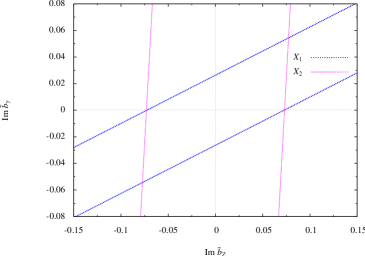
Figure 1: The region in the ${\mathrm{I}m}\tilde{b}_{Z}$-${\mathrm{I}m}\tilde{b}_{\gamma}$ plane accessible at the $95$% CL with observables $X_{1}$ and $X_{2}$ with unpolarized beams for integrated luminosity $L=250$ fb^-1.

For $X_{3}$ and $X_{4}$ we can draw a figure analogous to Fig.1 these couplings which would lead to the simultaneous limits

$$|{\mathrm{R}e}\tilde{b}_{Z}|\leq 6.08\times 10^{-2},|{\mathrm{R}e}\tilde{b}_{\gamma}|\leq 1.12\times 10^{-1}$$ (5)

Similarly, the simultaneous limits obtained from the observables $X_{5}$ and $X_{6}$ are

$$|{\mathrm{I}m}b_{Z}|\leq 1.25\times 10^{-1},\;|{\mathrm{I}m}b_{\gamma}|\leq 9.39\times 10^{-2}$$ (6)

Simultaneous limits on ${\mathrm{R}e}b_{Z}$ and ${\mathrm{R}e}b_{\gamma}$ from $X_{7}$ and $X_{8}$ are large since slopes of two lines corresponding to $X_{7}$ and $X_{8}$ are of same sign and approximately equal in magnitude.

${\mathrm{I}m}\Delta a_{Z}$, ${\mathrm{I}m}a_{\gamma}$ do not appear in the differential cross section. ${\mathrm{R}e}\Delta a_{Z}$ and ${\mathrm{R}e}a_{\gamma}$ too cannot be determined from $X_{7}$ and $X_{8}$. This is because in the determination of $\langle X_{7,8}\rangle\equiv\int X_{7,8}d\sigma/\sigma$, the contribution of ${\mathrm{R}e}\Delta a_{Z}$ to the numerator is cancelled exactly by its contribution at the linear order to the denominator. A similar cancellation takes place for ${\mathrm{R}e}a_{\gamma}$ approximately.

4.2 Sensitivities with longitudinal beam polarization

We now consider measurement of correlations with different combinations of longitudinal polarization. Since these would give different combinations of couplings, their measurements may be used to put simultaneous limits on couplings, without assuming any coupling to be zero.

A graphical way of obtaining simultaneous limits with different combinations of polarization is illustrated for $X_{1}$ in Fig.2 where relation eq. (3) is plotted in the space of the couplings involved for unpolarized beams denoted by $(0,0)$, and for the two combinations of longitudinal polarizations $(P_{L},\overline{P}_{L})\equiv(0.8,-0.6)$, and $(P_{L},\overline{P}_{L})\equiv(-0.8,0.6)$, respectively denoted by $(+,-)$ and $(-,+)$. The lines corresponding to any two combinations gives a closed region which is the allowed region at $95\%$ CL. In principle, allowed regions with other combinations of polarization can also be plotted, and the smallest region would correspond to the best limits.

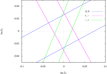
Figure 2: The region in the ${\mathrm{I}m}\tilde{b}_{Z}$-${\mathrm{I}m}\tilde{b}_{\gamma}$ plane accessible at the $95$% CL with observable $X_{1}$ with different beam polarization configurations. $(0,0)$, $(+,-)$ and $(-,+)$ stand for $(P_{L},\overline{P}_{L})=$ $(0,0)$, $(0.8,-0.6)$ and $(-0.8,0.6)$ respectively.

We note that certain observables get contribution from combinations like $g_{V}-g_{A}P^{\rm eff}_{L}$ in case of certain $\gamma ZH$ couplings or $2g_{V}g_{A}-(g_{V}^{2}+g_{A}^{2})P^{\rm eff}_{L}$ in case of certain $ZZH$ couplings, where $g_{V},g_{A}$ are the vector and axial-vector couplings of the $Z$ to charged leptons. In these cases, the sensitivity of those couplings to longitudinal polarization is high for the reason that the polarization dependent term gets an enhancement factor of $(g_{V}^{2}+g_{A}^{2})/(2g_{V}g_{A})\approx-4.2$, or $g_{A}/g_{V}\approx 8.3$ as compared to the unpolarized term, for the cases of $ZZH$ and $\gamma ZH$ couplings, respectively. This enhancement occurs for couplings ${\mathrm{I}m}\tilde{b}_{Z}$ for $X_{1}$, ${\mathrm{I}m}\tilde{b}_{\gamma}$ for $X_{2}$, ${\mathrm{R}e}\tilde{b}_{Z}$ for $X_{3}$, ${\mathrm{R}e}\tilde{b}_{\gamma}$ for $X_{4}$, ${\mathrm{I}m}b_{\gamma}$ for $X_{5}$, ${\mathrm{I}m}b_{Z}$ for $X_{6}$, and ${\mathrm{R}e}b_{\gamma}$ for $X_{7}$ and $X_{8}$.

We list in Table 2 the simultaneous limits which can be obtained using different combinations of polarizations for the various observables.

		Limit on coupling for the
Observable	Coupling	polarization combination
		$(0,0),(-,+)$	$(0,0),(+,-)$	$(-,+),(+,-)$
$X_{1}$	${\mathrm{I}m}\tilde{b}_{Z}$	$4.50\times 10^{-2}$	$3.59\times 10^{-2}$	$2.14\times 10^{-2}$
	${\mathrm{I}m}\tilde{b}_{\gamma}$	$4.28\times 10^{-2}$	$2.74\times 10^{-2}$	$3.04\times 10^{-2}$
$X_{2}$	${\mathrm{I}m}\tilde{b}_{Z}$	$9.73\times 10^{-2}$	$7.56\times 10^{-2}$	$8.54\times 10^{-2}$
	${\mathrm{I}m}\tilde{b}_{\gamma}$	$3.06\times 10^{-1}$	$2.19\times 10^{-1}$	$1.37\times 10^{-1}$
$X_{3}$	${\mathrm{R}e}\tilde{b}_{Z}$	$1.54\times 10^{-1}$	$1.22\times 10^{-1}$	$7.29\times 10^{-2}$
	${\mathrm{R}e}\tilde{b}_{\gamma}$	$1.46\times 10^{-1}$	$9.31\times 10^{-2}$	$1.08\times 10^{-1}$
$X_{4}$	${\mathrm{R}e}\tilde{b}_{Z}$	$5.37\times 10^{-2}$	$6.89\times 10^{-2}$	$6.10\times 10^{-2}$
	${\mathrm{R}e}\tilde{b}_{\gamma}$	$1.56\times 10^{-1}$	$2.18\times 10^{-1}$	$9.78\times 10^{-2}$
$X_{5}$	${\mathrm{I}m}b_{Z}$	$1.67\times 10^{-1}$	$1.29\times 10^{-1}$	$1.48\times 10^{-1}$
	${\mathrm{I}m}b_{\gamma}$	$5.27\times 10^{-1}$	$3.76\times 10^{-1}$	$2.36\times 10^{-1}$
$X_{6}$	${\mathrm{I}m}b_{Z}$	$7.79\times 10^{-2}$	$6.18\times 10^{-2}$	$3.69\times 10^{-2}$
	${\mathrm{I}m}b_{\gamma}$	$7.39\times 10^{-2}$	$4.72\times 10^{-2}$	$5.27\times 10^{-2}$
$X_{7}$	${\mathrm{R}e}b_{Z}$	$2.53\times 10^{-2}$	$1.27\times 10^{-2}$	$3.11\times 10^{-2}$
	${\mathrm{R}e}b_{\gamma}$	$1.05\times 10^{-1}$	$5.74\times 10^{-2}$	$5.11\times 10^{-2}$
$X_{8}$	${\mathrm{R}e}b_{Z}$	$2.58\times 10^{-2}$	$2.05\times 10^{-2}$	$3.37\times 10^{-2}$
	${\mathrm{R}e}b_{\gamma}$	$1.15\times 10^{-1}$	$6.33\times 10^{-2}$	$5.26\times 10^{-2}$

Table 2: Simultaneous $95$ % C.L. limits on the anomalous $ZZH$ and $\gamma ZH$ couplings from various observables using longitudinally polarized beams with different polarization combinations $(0,0)$, i.e., $P_{L}=0,\overline{P}_{L}=0$, $(\pm,\mp)$, i.e., $(P_{L}=\pm 0.8,\overline{P}_{L}=\mp 0.6)$ for $\sqrt{s}=500$ GeV and integrated luminosity $\int\mathcal{L}~{}dt=500$ fb^-1.

4.3 Sensitivities with transverse beam polarization

As observed earlier, observables $Y_{i}$ have vanishing expectation values in the absence of transverse polarization. We now discuss the effect of transverse polarization on these observables, which did not figure in the earlier discussion. Terms in the differential cross section dependent on transverse polarization have the combination $P_{T}\overline{P}_{T}$, and hence both beams need to have non-zero polarization to observe the effects of these terms.

We have listed in Table 3 the results for individual limits obtained following the procedures followed earlier.The most significant result is for the coupling ${\mathrm{I}m}a_{\gamma}$. We find that the observable $Y_{1}$ can constrain ${\mathrm{I}m}a_{\gamma}$ independent of all other couplings. This is particularly significant because ${\mathrm{I}m}a_{\gamma}$ cannot be constrained with longitudinal polarization. In the determination of $\langle Y_{2}\rangle$ the numerator receives contribution only from ${\mathrm{R}e}\Delta a_{Z}$ and ${\mathrm{R}e}a_{\gamma}$. However, the denominator at the linear order cancels the contribution of ${\mathrm{R}e}\Delta a_{Z}$ exactly and that of ${\mathrm{R}e}a_{\gamma}$ approximately, while introducing a dependence of $\langle Y_{2}\rangle$ on ${\mathrm{R}e}b_{Z}$ and ${\mathrm{R}e}b_{\gamma}$.

			Limits for polarizations
Observable		Coupling	$P_{T}=0.8$,  $\overline{P}_{T}=\pm 0.6$
$Y_{1}$	$(q_{x}q_{y})$	${\mathrm{I}m}a_{\gamma}$	$1.98\times 10^{-1}$
$Y_{2}$	$(q_{x}^{2}-q_{y}^{2})$	${\mathrm{R}e}a_{\gamma}$	$8.15\times 10^{-1}$
		${\mathrm{R}e}b_{Z}$	$2.65\times 10^{-2}$
		${\mathrm{R}e}b_{\gamma}$	$3.41\times 10^{-1}$
$Y_{3}$	$(p_{l^{-}}-p_{l^{+}})_{x}(p_{l^{-}}-p_{l^{+}})_{y}$	${\mathrm{I}m}a_{\gamma}$	$9.62$
		${\mathrm{I}m}b_{\gamma}$	$4.72\times 10^{-2}$
$Y_{5}$	$(p_{l^{-}}-p_{l^{+}})_{x}(p_{l^{-}}-p_{l^{+}})_{y}q_{z}$	${\mathrm{R}e}\tilde{b}_{Z}$	$5.56\times 10^{-2}$
		${\mathrm{R}e}\tilde{b}_{\gamma}$	$6.89\times 10^{-1}$
$Y_{4}$	$q_{x}q_{y}(p_{l^{-}}-p_{l^{+}})_{z}$	$\mathrm{I}mb_{Z}$	$1.58\times 10^{-1}$
		$\mathrm{I}mb_{\gamma}$	$1.96$
$Y_{6}$	$[(p_{l^{-}})_{x}^{2}-(p_{l^{+}})_{x}^{2}]-[(p_{l^{-}})_{y}^{2}-(p_{l^{+}})_{y}^{2}]$	${\mathrm{I}m}\tilde{b}_{Z}$	$1.10\times 10^{-1}$
		${\mathrm{I}m}\tilde{b}_{\gamma}$	$1.36$

Table 3: The $95$ % C.L. limits on the anomalous $ZZH$ and $\gamma ZH$ couplings, chosen nonzero one at a time from observables with transversely polarized beams for $\sqrt{s}=500$ GeV and $\int\mathcal{L}~{}dt=500$ fb^-1.

The other observables listed in Table 3 do not allow limits on single couplings to be isolated. However, in each of these cases, if one assumes the couplings contributing to the expectation value to be of the same order of magnitude, then one of the couplings make a dominant contribution to the expectation value, leading to an independent limit on that coupling. For example, $Y_{2}$, $Y_{3}$, $Y_{4}$, $Y_{5}$ and $Y_{6}$ can place independent limits on ${\mathrm{R}e}b_{Z}$, ${\mathrm{I}m}b_{\gamma}$, ${\mathrm{R}e}\tilde{b}_{Z}$, ${\mathrm{I}m}b_{Z}$ and ${\mathrm{I}m}\tilde{b}_{Z}$, respectively.

4.4 Effect of cuts and change in centre-of-mass energy

Since the anomalous couplings $b_{Z}$, $b_{\gamma}$, $\tilde{b}_{Z}$ and $\tilde{b}_{\gamma}$ corresponding to interactions which are momentum dependent, it is expected that a change in the c.m. energy would bring about a change in the sensitivity. To investigate this possibility, we have obtained sensitivities of all the observables to the anomalous couplings at two other center of mass energies i.e., $\sqrt{s}=800$ GeV with integrated luminosity $\int\mathcal{L}~{}dt=500$ fb^-1 and $\sqrt{s}=1000$ GeV with integrated luminosity $\int\mathcal{L}~{}dt=1000$ fb^-1.

We find that $X_{1}$, $X_{2}$ and $Y_{6}$ become less sensitive to couplings ${\mathrm{I}m}\tilde{b}_{Z}$ and ${\mathrm{I}m}\tilde{b}_{\gamma}$ as the c.m. energy increases. However, we have better limits at $\sqrt{s}=1000$ GeV than at $\sqrt{s}=800$ GeV, because the reduced sensitivity is compensated for by higher luminosity at $\sqrt{s}=1000$ GeV. $X_{3}$, $X_{4}$, $X_{5}$ and $Y_{4}$ are more sensitive to anomalous couplings at higher energies. $X_{7}$ becomes less sensitive to couplings ${\mathrm{R}e}b_{Z}$ and ${\mathrm{R}e}b_{\gamma}$ while $X_{8}$ gives better limits to these couplings at higher energies. Observables $Y_{1}$, $Y_{2}$ and $Y_{5}$ become less sensitive to anomalous couplings at higher energies. $Y_{3}$ behaves differently relative to all other observables. While the limit on ${\mathrm{I}m}a_{\gamma}$ improves by about an order of magnitude, the limit on ${\mathrm{I}m}b_{\gamma}$ get worse with increase in c.m. energy.

In practice, any measurement will need kinematical cuts for the identification of the decay leptons. We have examined the effect on our results of the following kinematical cuts [6]:

1. $E_{f}\geq 10$ GeV for each outgoing charged lepton,
2. $5^{\circ}\leq\theta_{0}\leq 175^{\circ}$ for each outgoing charged lepton to remain away from the beam pipe,
3. $\Delta R_{ll}\geq 0.2$ for the pair of charged lepton, where $(\Delta R)^{2}\equiv(\Delta\phi)^{2}+(\Delta\eta)^{2}$, $\Delta\phi$ and $\Delta\eta$ being the separation in azimuthal angle and rapidity, respectively, for detection of the two leptons as separated.

In addition to this, we impose a cut $|m_{l^{-}l^{+}}-M_{Z}|\leq 5\Gamma_{Z}$ on the invariant mass $m_{l^{-}l^{+}}$ of the lepton pair, so as to constrain the $Z$ - boson to be more or less on shell. This cut would allow us to test how well our results would simulate the results for a genuinely on-shell $Z$. Moreover, the cut would also reduce contamination from $\gamma\gamma H$ couplings, which contribute in principle to the process (2), though not to $e^{+}e^{-}\to HZ$.

After imposing these cuts, we find that all observables except $X_{1}$, $X_{2}$ and $Y_{6}$ are not very sensitive to these cuts. The limit on $X_{1}$, $X_{2}$ and $Y_{6}$ change by $20-30$%.

5 Conclusions and discussion

We have obtained angular distributions for the process $e^{+}e^{-}\to ZH\to\ell^{+}\ell^{-}H$ in the presence of anomalous $\gamma ZH$ and $ZZH$ couplings to linear order in these couplings in the presence of longitudinal and transverse beam polarizations. We have then looked at observables which can be used in combinations to disentangle the various couplings to the extent possible. We have also obtained the sensitivities of these observables and asymmetries to the various couplings for a definite configuration of the linear collider.

In certain cases where the contribution of a coupling is suppressed due to the fact that the vector coupling of the $Z$ to $e^{+}e^{-}$ is numerically small, longitudinal polarization helps to enhance the contribution of this coupling. As a result, longitudinal polarization improves the sensitivity. The main advantage of transverse polarization is that it enables constraining ${\mathrm{I}m}a_{\gamma}$ which is not accessible without transverse polarization. Moreover, it helps to determine certain couplings independent of all other couplings.

We find that with a linear collider operating at a c.m. energy of 500 GeV with the capability of 80% electron polarization and 60% positron polarization with an integrated luminosity of 500 fb^-1, with the observables described above, it would be possible to place 95% CL individual limits of the order of a few times $10^{-2}$ on all couplings taken nonzero one at a time with use of an appropriate combination ($P_{L}$ and $\overline{P}_{L}$ of opposite signs) of longitudinal beam polarizations. This is an improvement by a factor of 5 to 10 as compared to the unpolarized case. The simultaneous limits possible are, as expected, less stringent. While they continue to be better than $5\times 10^{-2}$ for most couplings, they range between $5\times 10^{-2}$ and about $10^{-1}$ for ${\mathrm{R}e}b_{\gamma}$, ${\mathrm{R}e}\tilde{b}_{Z}$ and ${\mathrm{R}e}\tilde{b}_{\gamma}$. Transverse polarization enables the determination of ${\mathrm{I}m}a_{\gamma}$ independent of all other couplings, with a possible 95% CL limit of about 0.2. Independent limits on ${\mathrm{R}e}b_{Z}$ and ${\mathrm{I}m}b_{\gamma}$ of a few times $10^{-2}$ are possible, whereas those on ${\mathrm{I}m}b_{Z}$, ${\mathrm{R}e}\tilde{b}_{Z}$ and ${\mathrm{I}m}\tilde{b}_{Z}$ would be somewhat larger, ranging upto about 0.1. Our procedure does not permit any limit on ${\mathrm{R}e}\Delta a_{Z}$ or ${\mathrm{I}m}\Delta a_{Z}$, and only a weak limit on ${\mathrm{R}e}a_{\gamma}$.

We have assumed that only one leptonic decay mode of $Z$ is observed. Including both $\mu^{+}\mu^{-}$ and $\tau^{+}\tau^{-}$ modes would trivially improve the sensitivity. In case of observables like $X_{1}$, $Y_{1}$, $Y_{2}$, which do not need charge identification, even hadronic decay modes of $Z$ can be included, which would considerably enhance the sensitivity.

In fact, in our earlier work [9], where we had not included $Z$ decay, the sensitivities we obtained were better simply because we did not restrict to one decay channel. On the other hand, considering a specific charged-lepton channel has enabled us to get a handle on ${\mathrm{I}m}b_{\gamma}$, ${\mathrm{I}m}b_{Z}$, ${\mathrm{R}e}\tilde{b}_{\gamma}$ and ${\mathrm{R}e}\tilde{b}_{Z}$, which were not accessible in [9].

It is appropriate to compare our results with those in works using the same parameterization as ours for the anomalous coupling and with an approach similar to ours. The paper of Han and Jiang [5] deals with CP-violating $ZZH$ couplings, and it is possible to compare the 95% CL limits on ${\mathrm{I}m}\tilde{b}_{Z}$ with those obtained by them using the forward-backward asymmetry of the $Z$. With identical values of $\sqrt{s}$ and integrated luminosity, Han and Jiang quote limits of 0.019 and 0.0028 for ${\mathrm{I}m}\tilde{b}_{Z}$, respectively for unpolarized and longitudinally polarized beams with opposite-sign $e^{+}$ and $e^{-}$ polarizations. The corresponding numbers we have from $X_{1}$ are 0.041 and 0.0099. The agreement is reasonable, after taking into account the facts that we use only one leptonic channel, and that they employ additional experimental cuts. The papers in [6] also deal only with anomalous $ZZH$ couplings, and quote $3\sigma$ limits on the couplings. The $3\sigma$ limit they quote for ${\mathrm{I}m}\tilde{b}_{Z}$ is $0.064$ for unpolarized beams, and $0.0089$ for polarized beams. After correcting for the CL limit of $1.96\sigma$ which we use, and the inclusion of a single leptonic decay mode, their limits are still somewhat worse. This could be attributed to the stringent kinematic cuts imposed by them, and to the different luminosity choice in the case of polarized beams. Similarly, the limits quoted in [6] for ${\mathrm{R}e}b_{Z}$ and ${\mathrm{I}m}b_{Z}$ are worse compared to ours by a factor of order 2 or 3 in the unpolarized as well as cases of longitudinal and transverse polarization.

As for the case of $\gamma ZH$ couplings, comparison with earlier work is not easy because of the different approach to parameterization of couplings. Also, there is no work dealing in transverse polarization with which we could make a comparison.

In the above, we have assumed a Higgs mass of 120 GeV. For larger values of $m_{H}$, for larger Higgs masses, we find somewhat decreased sensitivities. We have also studied the sensitivities at higher c.m. energies, possibly with a higher luminosity, and find that in case of some observables, the sensitivity improves with simultaneous increase in energy and luminosity.

We have not included the decay of the Higgs boson in our analysis. For now, one could simply divide our limits by the square root of the branching ratios and detection efficiencies. Including the decay will entail some loss of efficiency.

While some of these practical questions are not addressed in this work, we feel that the interesting new features we found would make it worthwhile to address them in future.

References

- [1] A. Djouadi, J. Lykken, K. Monig, Y. Okada, M. J. Oreglia, S. Yamashita et al., arXiv:0709.1893 [hep-ph].
- [2] V. D. Barger, K. m. Cheung, A. Djouadi, B. A. Kniehl and P. M. Zerwas, Phys. Rev. D 49, 79 (1994); W. Kilian, M. Kramer and P. M. Zerwas, arXiv:hep-ph/9605437; Phys. Lett. B 381, 243 (1996); J. F. Gunion, B. Grzadkowski and X. G. He, Phys. Rev. Lett. 77, 5172 (1996); M. C. Gonzalez-Garcia, S. M. Lietti and S. F. Novaes, Phys. Rev. D 59, 075008 (1999); V. Barger, T. Han, P. Langacker, B. McElrath and P. Zerwas, Phys. Rev. D 67, 115001 (2003).
- [3] K. Hagiwara and M. L. Stong, Z. Phys. C 62, 99 (1994); G. J. Gounaris, F. M. Renard and N. D. Vlachos, Nucl. Phys. B 459, 51 (1996).
- [4] K. Hagiwara, S. Ishihara, J. Kamoshita and B. A. Kniehl, Eur. Phys. J. C 14, 457 (2000); S. Dutta, K. Hagiwara and Y. Matsumoto, Phys. Rev. D 78, 115016 (2008).
- [5] A. Skjold and P. Osland, Nucl. Phys. B 453, 3 (1995). T. Han and J. Jiang, Phys. Rev. D 63, 096007 (2001).
- [6] S. S. Biswal, R. M. Godbole, R. K. Singh and D. Choudhury, Phys. Rev. D 73, 035001 (2006) [Erratum-ibid. D 74, 039904 (2006)]; S. S. Biswal, D. Choudhury, R. M. Godbole and Mamta, Phys. Rev. D 79, 035012 (2009); S. S. Biswal and R. M. Godbole, Phys. Lett. B 680, 81 (2009)
- [7] Q. H. Cao, F. Larios, G. Tavares-Velasco and C. P. Yuan, Phys. Rev. D 74, 056001 (2006).
- [8] K. Rao and S. D. Rindani, Phys. Lett. B 642, 85 (2006); Phys. Rev. D 77, 015009 (2008).
- [9] S. D. Rindani and P. Sharma, Phys. Rev. D 79, 075007 (2009).
- [10] D. Atwood and A. Soni, Phys. Rev. D 45, 2405 (1992).
- [11] G. Moortgat-Pick et al., Phys. Rept. 460, 131 (2008).
- [12] B. Ananthanarayan and S. D. Rindani, Phys. Rev. D 70, 036005 (2004); B. Ananthanarayan, S. D. Rindani, R. K. Singh and A. Bartl, Phys. Lett. B 593, 95 (2004) [Erratum-ibid. B 608, 274 (2005)]; B. Ananthanarayan and S. D. Rindani, Phys. Lett. B 606, 107 (2005); JHEP 0510, 077 (2005); S. D. Rindani, Phys. Lett. B 602, 97 (2004); A. Bartl, H. Fraas, S. Hesselbach, K. Hohenwarter-Sodek, T. Kernreiter and G. Moortgat-Pick, JHEP 0601, 170 (2006); S. Y. Choi, M. Drees and J. Song, JHEP 0609, 064 (2006); K. Huitu and S. K. Rai, Phys. Rev. D 77, 035015 (2008); R. M. Godbole, S. K. Rai and S. D. Rindani, Phys. Lett. B 678, 395 (2009).
- [13] P. Poulose and S. D. Rindani, Phys. Lett. B 383, 212 (1996); Phys. Rev. D 54, 4326 (1996) [Erratum-ibid. D 61, 119901 (2000)]; Phys. Lett. B 349, 379 (1995); F. Cuypers and S. D. Rindani, Phys. Lett. B 343, 333 (1995); D. Choudhury and S. D. Rindani, Phys. Lett. B 335, 198 (1994); S. D. Rindani, Pramana 61, 33 (2003).
- [14] J. A. M. Vermaseren, arXiv:math-ph/0010025.
- [15] P. Ciafaloni, D. Comelli and A. Vergine, JHEP 0407, 039 (2004).
- [16] K.-i. Hikasa, Phys. Rev. D 33, 3203 (1986).