Maxwell-Drude-Bloch dissipative few-cycle optical solitons

Abstract

We study the propagation of few-cycle pulses in two-component medium consisting of nonlinear amplifying and absorbing two-level centers embedded into a linear and conductive host material. First we present a linear theory of propagation of short pulses in a purely conductive material, and demonstrate the diffusive behavior for the evolution of the low-frequency components of the magnetic field in the case of relatively strong conductivity. Then, numerical simulations carried out in the frame of the full nonlinear theory involving the Maxwell-Drude-Bloch model reveal the stable creation and propagation of few-cycle dissipative solitons under excitation by incident femtosecond optical pulses of relatively high energies. The broadband losses that are introduced by the medium conductivity represent the main stabilization mechanism for the dissipative few-cycle solitons.

I Introduction

Few-cycle optical pulses with durations of only a few periods of the optical radiation BK ; DGC dramatically expand the horizon of modern optics, and offer new applications in metrology, ultrafast spectroscopy, and material processing. Such pulses are of particular relevance to the field of extreme nonlinear optics, where electromagnetic fields of enormously large intensities are required MTB . Optical soliton effects may play an important role in the process of generation of few-cycle pulses, as well as in the course of their propagation through nonlinear media. As a matter of fact, the appropriate description of few-cycle pulse generation and propagation reveals new, not previously anticipated physics, in parallel calling for the abandonment of most of the approximations which are of standard use in nonlinear optics, and for the development of new approaches to the treatment of the interaction of spectrally broadband radiation with matter.

To the best of our knowledge, the first example of conservative few-cycle soliton was found in the context of nonreduced Maxwell-Bloch equations by Bullough and Ahmad in Ref. BA_71 . That soliton was of the video type, that is with zero carrier frequency, with an hyperbolic secant shape for the total electric field of the pulse and not its envelope. More recent studies, see e.g. KSAHL ; AVB , have considered a new class of conservative few-cycle solitons which are the solutions of a properly generalized nonlinear Schroedinger equation, without the assumption of a slowly varying field envelope as well as the approximation of unidirectional propagation. The dispersive properties of the medium that was modeled in those studies imply the singularity of the dielectric constant at zero frequency, which leads to the area constraint $S_{E}\equiv\int_{-\infty}^{+\infty}dt\,E=0$ that was imposed on the electric field $E$ of any localized field distribution such as the soliton. This area constraint may appear to be violated in real-world experiments, whenever the zero-frequency component of the field is generated in a coherent source either spontaneously or deterministically, e.g., via optical rectification in a medium with quadratic nonlinearity. It is then natural to undertake the study of the dynamics of low-frequency Fourier components of the electromagnetic field in situations where the electric field area constraint is lifted: this is one of the goals that we will pursue in our present study.

Additionally, the above mentioned studies were devoted to the properties of conservative solitons, hence the effects of medium gain and loss were not considered. However, losses (as well as the gain which is necessary to balance them) come to the forefront whenever one sets the goal of generating few-cycle pulses, and possibly propagating them over long distances. Moreover, as well known, in active media it is exactly the frequency-dependence of gain (and loss) which determines the utmost degree of achievable pulse compression. Soliton type effects in combination with losses and gain give rise to localized field structures known as dissipative solitons, which are of primary interest in our study. Indeed, in our work we will exploit a full-scale analysis of the interaction of a strong few-cycle pulse with a dissipative medium consisting of a two-component (i.e., amplifying and absorbing) ensemble of two-level doping centers (atoms or quantum dots), embedded in a conductive host. In doing that, we will reject the usual approximation of slowly varying envelopes, as well as the unidirectional approximation and the approximation of zero electric area $S_{E}=0$. In short, in this paper we are going to investigate the formation of few-cycle dissipative solitons within the framework of the non-reduced Maxwell-Drude-Bloch equations.

Few-cycle dissipative solitons based on the phenomenon of the McCall and Hahn self-induced transparency McCall_67 ; McCall_69 were first theoretically studied in Refs. VRSFW ; VRS_06 . In those studies, the propagation medium was composed of two sorts of resonant atomic systems – absorbing and amplifying. The idea behind the formation of dissipative solitons is the following. In the absence of dissipative factors, such as loss and gain, a two-level resonant atomic system supports the formation of a conservative soliton. As well known, such solitons form a family of solutions, where the soliton peak amplitude is a continuously varying parameter. The temporal duration of these solitons is inversely proportional to their amplitude. If one now allows for the existence of a weak linear gain (a small dissipative factor), the propagation dynamics leads to a continuous transition with distance to solitons within the family with progressively higher amplitudes, and correspondingly shorter durations. In fact, the soliton amplitude grows exponentially with the propagation length, and its time duration also shortens exponentially: both factors work together and result in the temporal collapse of the soliton. At first sight, such shortening would be welcome as it produces high power, few-cycle pulses. However, such behavior is not realistic in practice, as it does not account for nonlinear, dispersive and absorptive mechanisms that work against the collapse, and that are inherently present in any real medium. Moreover, when only linear gain is present, (bright) localized structures appear to be unstable against amplification of perturbations on the tails of their field. When taking into account the nonlinearity of a two-level gain medium, which is supposed to be coupled with a relaxing two-level absorber, one observes the appearance of a set of localized few-cycle pulses with stationary shapes and exhibiting a discrete set of velocities, see Ref. VRSFW . Later on in Ref. VRS_06 it was shown that these localized pulses are not stable, since their collapse is not counterbalanced by the nonlinearity of the gain. Nevertheless, it was also predicted that stabilization of the soliton is possible by introducing a third level into the model of the absorbing medium. In this way, stable half-cycle (or video-) dissipative solitons were obtained and studied in detail, see Refs. VRS_06 ; RSV_07 ; RSV_08 . More recently, few-cycle dissipative solitons (containing several oscillations of the field) were found in Ref. VRS_09 for the model of amplifying and absorbing homogeneously as well as inhomogeneously broadened quantum dots, embedded into a quartz host material. In that work, the host matrix was modeled by means of a three-level system with two separate resonance frequencies located in the infra-red and in the ultra-violet spectral domains, respectively. In this way, the linear (absorptive and dispersive) properties of the host medium in its transparency region could be reproduced with high accuracy. For this model, it was of paramount importance (from the standpoint of practical applications) to observe that the few-cycle dissipative solitons could be excited by means of a much longer femtosecond pulse incident on the medium. Such soliton generation mechanism exhibits a threshold behavior: namely, low-intensity pulses disperse and decay, whereas the evolution of above-threshold pulses results in the formation of dissipative solitons. Note that the (nonstationary) propagation of a few-cycle pulse in a two-level amplifier was studied in Ref. T_OC , however without counterbalancing the gain by the nonlinearity as well as the linear or nonlinear losses of the absorber. Therefore the type of dissipative solitons which are of present interest to us cannot be formed in the configuration that was considered in Ref. T_OC .

All of the above-mentioned studies assume that the response of the medium to the electromagnetic field is solely described in terms of the medium polarization. However, according to the Lorentz electrodynamics of continuous media, the medium interaction with radiation is governed not only by the response of bound charges (electrons), i.e. medium polarization, but also by the response of free electrons, i.e., the electric current. In this paper we present a significant step forward in our studies of few-cycle dissipative optical solitons, by proposing a new approach that is based on the full Lorentz model, which eventually leads us to the formulation of the Maxwell-Drude-Bloch model. We demonstrate that such a model is appropriate for treating the medium of our interest, namely an ensemble of active (amplifying) and passive (absorbing) quantum dots embedded into a semiconductor, off-resonance host matrix. The semiconductor host material is characterized by an appreciable value of the electrical conductivity, which may be most easily regulated by a proper choice of the concentration of dopants. We demonstrate that conductivity provides a stabilization mechanism for dissipative solitons, even in the case where simple two-level models are used to describe active and passive quantum dots. As a matter of fact, the role of conductivity is two-fold. First of all, conductivity provides broadband (although tilted with frequency) linear losses, which are of vital importance for the stabilization of solitons. The second property (that is not related with soliton stabilization) of conductivity is that it leads to high reflectivity for

low-frequency field components in the experimental situation which is of interest for us, namely an electromagnetic pulse that is incident at the boundary with a conductive medium. As a matter of fact, in this situation the Fresnel reflectivity is unity for the zero-frequency component of the field. The role of conductivity has been so far under-appreciated in both linear and nonlinear optics, albeit for a good reason, namely because the carrier frequency of a laser pulse is so high and its spectrum is so narrow (with respect to the carrier frequency) that the zero-frequency component of the optical field has practically zero intensity. However, the situation changes when the pulse becomes as short as a few optical oscillations, or when it represents a video-pulse. In such situations, the zero-frequency component cannot be ignored anymore: the conductivity of semiconductor materials strongly affects the spectrum of both the propagating as well as the reflected pulse. As a consequence, we need to generalize the usual Maxwell-Bloch approach which describes the interaction of the electromagnetic field with bound electrons, in order to include its interaction with the medium free electrons. The dynamics of the latter is modeled by means of the Drude equation, so that the whole light-matter interaction picture must be based on the simultaneous solution of the Maxwell-Drude-Bloch equations (some relevant studies concerning the photovoltaic and photorefractive effects are presented in Ref. SF ).

Since the few-cycle dissipative solitons that we are going to investigate in this work have their roots back in the phenomenon of self-induced transparency, a related and significant subject of our discussion is the notion of the pulse area. For pulses of slowly varying envelopes, the pulse area was introduced as the time integral (between minus and plus infinity) over the pulse envelope. Such pulse envelope area obeys the celebrated McCall and Hahn Area Theorem, see McCall_69 . However, the notion of pulse envelope is no longer appropriate for few-cycle pulses: as a consequence, the Area Theorem is no longer valid, see Refs. H_98 ; T_OE . For few-cycle pulses, instead of the envelope area, it is appropriate to consider the electric field area, which is defined as the time integral with infinite limits of the electric field itself (and not its envelope). A simple equation governing evolution of the electric field area in a rather general medium was derived in Ref. R_09 . Physically, the electric field area represents the zero-frequency component of the Fourier spectrum of the electromagnetic field. Such a component is of no practical importance for narrowband optical pulses, since in this case we may suppose a vanishing zero-frequency field amplitude. Nevertheless, the electric field area may gain a valuable meaning in the case of ultra-broadband (few-cycle) pulses, where the zero-frequency component of the total field may no longer be negligible. In this work, we also introduce the notion of the area of the magnetic field, which is defined as the integral of the magnetic field over the spatial coordinate. In practice, such definition is more appropriate than the definition of the electric field area, since the evolution of the magnetic field area may be easily numerically computed when solving realistic initial-value problems, i.e., whenever the electromagnetic field is specified along the spatial coordinate, and time is the evolution coordinate.

In summary, the primary goal of this paper is the study of the propagation of few-cycle pulses through a two-component medium consisting of (nonlinear) amplifying and absorbing two-level centers (atoms or quantum dots), embedded into a (linear) host material that exhibits an appreciable value of electrical conductivity. Physically, we think of the host material as a semiconductor, since it can be manufactured with a high concentration of electrons in the conduction band. As appropriate candidates for the two-level absorbing and amplifying centers, we envisage the use of two different types of quantum dots, which possess huge dipole moments, so that one may avoid material breakdown by the otherwise highly intense field of the few-cycle pulse (note that the Rabi frequency can be as high as the optical frequency). The large nonlinearity of the quantum dots permits us to neglect the nonlinearity of the host semiconductor material. For the sake of simplicity, we also neglect in this work the dispersive properties of the host material, which can be introduced following the approach of Ref. VRS_09 , and whose presence does not affect the generality of the present results. We start our paper with a linear theory of propagation of short pulses in a purely conductive material (i.e., with no embedded two-level systems), a topic which has not yet received much attention in optics. Next we proceed to develop the nonlinear theory of propagation of few-cycle pulses in a conductive material that is doped with resonant amplifying and absorbing two-level doping centers. Finally, we conclude by providing extensive numerical simulation results demonstrating the stable formation and propagation of few-cycle dissipative solitons in the framework of the fully nonlinear Maxwell-Drude-Bloch model.

II Maxwell equations and the electromagnetic area

Let us consider a one-dimensional electromagnetic pattern of finite temporal and spatial extension. This can be for example a pulse propagating in a single-mode optical waveguide, in situations where the associated waveguide dispersion may be neglected, namely whenever the central part of the pulse spectrum is far from the mode cut-off frequency. In this case, it is possible to derive separate conservation laws for both the electric as well as the magnetic field area. Two of the Maxwell equations are relevant to us here. They read as

$$\nabla\times{\textbf{E}}=-\frac{1}{c}\frac{\partial{\textbf{B}}}{\partial t}\,,$$ (1)

$$\nabla\cdot{\textbf{B}}=0\,.$$ (2)

Here E and B are the strength of the electric field and of the magnetic induction, respectively, and $c$ is the speed of light in vacuum. In a one-dimensional geometry, the field strength only depends on one (longitudinal) coordinate, say, $z$ and on time $t$. Therefore, as it follows from Eq. (2), the $z$-component $B_{z}$ of the magnetic field is zero. Then, Eq. (1) takes the form

$$-\frac{\partial E_{y}}{\partial z}{\textbf{e}}_{x}+\frac{\partial E_{x}}{\partial z}{\textbf{e}}_{y}=-\frac{1}{c}\frac{\partial{\textbf{B}}_{\perp}}{\partial t}\,,$$ (3)

where ${\textbf{e}}_{x,y}$ are unit vectors in the Cartesian frame orthogonal to the propagation variable $z$, and ${\textbf{B}}_{\perp}=(B_{x},\,B_{y})^{T}$.

Next we define the magnetic area of the pulse as

$${\textbf{S}}_{B}(t)=\int_{-\infty}^{+\infty}dz\,{\textbf{B}}(z,t)\,.$$ (4)

Note that the longitudinal component of this vector is zero. Then, integrating Eq. (3) over the longitudinal coordinate $z$, one obtains the equation

$$\frac{d}{dt}{\textbf{S}}_{B}=0\,,$$ (5)

which is nothing but the conservation law for the magnetic area. That is, the amplitude of the zero-frequency (or dc) component of the Fourier spectrum of the magnetic field strength does not change with time. This law separately applies to both polarization eigenmodes of the field. Similarly, by introducing the electric field area of the electromagnetic pulse as

$${\textbf{S}}_{E}(z)=\int_{-\infty}^{+\infty}dt\,{\textbf{E}}_{\perp}(z,t)$$ (6)

we get

$$\frac{d}{dz}{\textbf{S}}_{E}=0\,,$$ (7)

after integration of Eq. (3) over time. The interpretation of the conservation law for the electric area as in Eq. (7) is, similar to the case of the magnetic area, the time-invariance of the dc component of the electric field. Note that in the course of the above derivations we did not explicitly use any material equation. Nevertheless, we supposed that the electric and magnetic fields vanish at the pulse tails. Generally speaking, this only happens in the presence of a relaxation in the material response to the electromagnetic field. In simplified models, whenever such relaxation is neglected, the above discussed area conservation properties do not hold. Unlike the area theorem of self-induced transparency, which was derived for a conservative two-level absorber, the conservation law for the electric and magnetic areas, see Eqs. (5) and (7), directly follows from Maxwell’s equations, without the necessity to provide any specification about the medium (that can even be inhomogeneous) where wave propagation occurs.

Next, let us involve in our considerations another Maxwell equation which provides a link to the optical properties of the material. We suppose the medium to be electrically neutral, i.e., with electric charge density $\rho=0$, and the electromagnetic field to be transverse, i.e. the longitudinal components of the electric field E, of the electric displacement D, and of the current density j, all vanish. In the adopted one-dimensional geometry, we arrive to the wave equation

$$\frac{\partial^{2}{\textbf{E}}_{\perp}}{\partial z^{2}}-\frac{4\pi}{c^{2}}\,\frac{\partial{\textbf{j}}_{\perp}}{\partial t}-\frac{1}{c^{2}}\,\frac{\partial^{2}{\textbf{D}}_{\perp}}{\partial t^{2}}=0\,.$$ (8)

Since we are also interested in studying the dynamics of low-frequency radiation in the conductive medium, it is instructive to analyze the behavior of pulses whose spectra lie in the vicinity of zero frequency. Then we may neglect the last term in Eq. (8) and also use the Ohm law for the current,

$${\textbf{j}}=\sigma_{0}{\textbf{E}}\,,$$ (9)

where $\sigma_{0}$ is the static conductivity of the medium. In the above limiting situation, the wave equation is transformed to the one-dimensional parabolic equation

$$\frac{4\pi\sigma_{0}}{c^{2}}\,\frac{\partial{\textbf{E}}_{\perp}}{\partial t}=\frac{\partial^{2}{\textbf{E}}_{\perp}}{\partial z^{2}}\,.$$ (10)

Similar equation holds for the magnetic induction ${\textbf{B}}_{\perp}$, see e.g. Jackson . Such type of equation is quite unusual for describing optical phenomena. Indeed, Eq. (10) is mostly applicable to video-pulses rather than to narrowband or even few-cycle optical pulses, also in the THz region. On the other hand, Eq. (10) is widely known in the theory of heat conductivity and diffusion, CJ and also in the description of quasi-static electromagnetic fields, Foucault currents and skin effect in conductors LL .

The above derived parabolic equation is valid whenever the following inequalities are satisfied:

$$\omega\ll\nu\,,\quad\omega\ll 4\pi\sigma_{0}\,,\quad\omega\ll 4\pi\sigma_{0}/|\epsilon_{0}|\,,$$ (11)

where $\nu$ is the effective frequency of collisions of free electrons with ions and atoms, and $\epsilon_{0}$ is the static component of the dielectric permittivity, possibly including a nonlinear contribution. Since for most situations $|\epsilon_{0}|\sim 1$, the last inequality in Eq. (11) can be omitted. If we come back to the original Maxwell’s equations and estimate the value of the electric field strength versus the magnetic field strength in such regime, we arrive at an interesting inequality

$$E\sim\sqrt{\frac{\omega}{4\pi\sigma_{0}}}H\ll H\,.$$ (12)

Namely, the electromagnetic field of a low-frequency pulse in a highly conductive material mainly consists of the magnetic field, in contrast to dielectrics where magnetic and electric fields are of comparable strength.

In practical situations involving relatively large observation times, the detailed form of the initial and boundary conditions for the diffusion equation (10) may become irrelevant, and we may consider the medium as infinite. Let us briefly overview the main characteristics of the field diffusion process in an infinite medium. As a field, we take the magnetic component B of the electromagnetic field. This choice is dictated at first by the dominance of the magnetic field over the electric field as expressed by Eq. (12). Moreover, as we shall see in the following, this choice has interesting consequences in our discussion of the evolution of the magnetic area, and leads to a better (when compared with the electric field) correlation with the analytically tractable case of “transparent” boundary conditions. For an infinite medium, we may introduce $n$-th momentum of the field ($n=0,\,1,\,2,\,\dots$) according to the formula

$${\textbf{S}}_{n}(t)=\int_{-\infty}^{\infty}dz\,z^{n}{\textbf{B}}_{\perp}(z,\,t)\,.$$ (13)

Note that zeroth momentum coincides with the definition of the magnetic area given in Eq. (4). Substituting these definitions into the diffusion equation (10), we get for first three momenta

$$\frac{d{\textbf{S}}_{0}}{dt}=\frac{d{\textbf{S}}_{1}}{dt}=0\,,$$ (14)

$$\frac{d{\textbf{S}}_{2}}{dt}=2D{\textbf{S}}_{0}\,,$$ (15)

where $D=c^{2}/4\pi\sigma_{0}$ is the diffusion coefficient. The conservation of the zeroth momentum is a consequence of a more general area theorem (5) for the magnetic field. The conservation of the first momentum means that the centers of the magnetic distributions defined for corresponding polarizations as $Z_{x}=S_{1x}/S_{0x}$ and $Z_{y}=S_{1y}/S_{0y}$ do not move in the course of the diffusion. In its turn, the evolution of the second momentum reflects the broadening of the magnetic field distribution with time. Namely, the width of the distribution grows larger in proportion to $(t-t_{0})^{1/2}$. Bearing in mind the conservation of the zeroth momentum, we may conclude that the amplitude of the distribution correspondingly decreases as $(t-t_{0})^{-1/2}$. When compared with the standard exponential decay of the field in an absorbing medium, in this case the dynamics of the magnetic field evolution is extremely slow (power-law decay). The above discussed behavior of the first three momenta of the field is typical of any diffusion process in an infinite medium. For asymptotically large evolution times $t$, the memory of any particular initial condition at $t=0$ dies out, and the field evolves self-similarly as

$${\textbf{B}}_{\perp}\propto\frac{1}{[D(t-t_{0})]^{1/2}}\,\exp\left[-\frac{z^{2}}{4D(t-t_{0})}\right]\,,$$ (16)

where $t_{0}$ is arbitrary an instant in time that is asymptotically far from $t=0$.

More relevant to our present study of the propagation of pulses incident on the boundary with a conductive material is the consideration of the corresponding boundary-value problem. Let us consider first the analytically tractable case of “transparent” boundary, i.e. a boundary which is transparent for low-frequency radiation. We assume that the initial pulse that is incident on the boundary with the semi-infinite medium at $t=0$ has already diffused sufficiently deep into the medium, so that the value of B at the boundary (located at $z=0$) has become vanishing small. In this asymptotic limit, the field evolves self-similarly as

$${\textbf{B}}_{\perp}\propto\frac{1}{[D(t-t_{0})]^{3/2}}\,\exp\left[-\frac{z^{2}}{4D(t-t_{0})}\right]$$ (17)

for $z\geq 0$. In order to accomodate the definitions of the momenta given in Eq. (13) to the case of a semi-infinite medium, we change in these expressions the lower integration limits to $0$, and supply such re-defined momenta by the superscript $(tr)$ (standing for transmitted). Then, as a result of the escape of the field into vacuum the zeroth order momentum (magnetic area of the transmitted field) is no longer conserved. As a matter of fact, for asymptotically large times the transmitted magnetic area decays as ${\textbf{S}}_{0}^{(tr)}\propto(t-t_{0})^{-1/2}$. However, the first order momentum is still conserved, therefore the centers of gravities of the field distributions $Z_{x}$ and $Z_{y}$ penetrate deeper and deeper into the medium as time evolves [$\propto(t-t_{0})^{1/2}$]. However, the speed of this motion slows down with time with a the rate proportional to $(t-t_{0})^{-1/2}$. Although the real boundary conditions in our present model have a more complicated form, nevertheless in the next section we will make use of the above discussed asymptotic diffusive time-dependency of the low-frequency components of the magnetic field, in order to demonstrate its diffusive behavior in a highly conductive medium.

Leaving the parabolic equation (10) aside for the time being, let us return to the wave equation (8). We do not assume anymore that the conductivity acquires extreme values. Therefore both material terms in the wave equation should be considered on equal footing. For low-intensity pulses a linear propagation theory is readily applicable. The evolution of each Fourier component of the electromagnetic pulse can be represented by a running plane wave

$${\textbf{E}}_{\perp}=\mbox{Re}\left\{{\textbf{E}}_{\omega}\exp[i(kz-\omega t)]\right\}\,.$$ (18)

Similar decompositions take place for the current and the electric induction:

$${\textbf{j}}_{\perp}=\mbox{Re}\left\{{\sigma(\omega)\textbf{E}}_{\omega}\exp[i(kz-\omega t)]\right\}\,.$$ (19)

$${\textbf{D}}_{\perp}=\mbox{Re}\left\{{\varepsilon(\omega)\textbf{E}}_{\omega}\exp[i(kz-\omega t)]\right\}\,.$$ (20)

where both the frequency-dependent complex-valued conductivity $\sigma(\omega)$ and the dielectric permittivity $\varepsilon(\omega)$ depend on the model in use. Upon substitution of the decompositions (18)-(20) into the wave equation (8), one obtains the dispersion relation of the wave number in the form

$$k(\omega)=\pm\sqrt{\frac{\omega^{2}}{c^{2}}\,\varepsilon(\omega)+i\frac{4\pi\omega}{c^{2}}\,\sigma(\omega)}\,.$$ (21)

The two signs before the square root correspond to the two opposite directions of wave propagation. Since we are interested in soliton dynamics, our model will be a nonlinear one. However, the linear theory is still valuable because it allows us to check the stability of a dissipative soliton against the undesirable amplification of low-intensity field perturbations to the soliton tails. As a matter of fact, the stability of any (bright) localized nonlinear field structure or pulse requires the trivial solution (${\textbf{E}}=0$) of the wave equation (8) to be also stable. Otherwise, the pulse tails will grow up exponentially in their propagation, so that the localized structure is also unstable. Formally, the stability of the trivial solution means that the small-signal gain coefficient does not exceed the small-signal absorption coefficient at any frequency $\omega$. As soon as we will complete the description of our model and define the functions $\sigma(\omega)$ and $\varepsilon(\omega)$, we will come back to this problem and check the stability of the trivial solution ${\textbf{E}}=0$.

III The Drude equation and the Maxwell-Drude model

Let us start the introduction of the material equations with an equation for the electric current. According to the Lorentz macroscopic electrodynamic theory, a medium contains two types of charges (electrons) – bound and free, LL . The dynamics of bound charges is described by a (generally, nonlinear) polarization, whose evolution is governed by the equations for the density matrix (or Bloch equations). In our case, these equations describe two types of two-level atom-like systems – amplifying and absorbing centers. The corresponding equations will be presented in the next section. Here we concentrate on the dynamics of free charges, and follow the equation of motion for the current as it was proposed by Drude. This equation reads as

$$\frac{d{\textbf{j}_{\perp}}}{dt}+\nu{\textbf{j}}_{\perp}=\frac{\omega_{p}^{2}}{4\pi}\,{\textbf{E}}_{\perp}\,.$$ (22)

Here $\omega_{p}^{2}=4\pi e^{2}N_{e}/m_{e}$ is the square of the plasma frequency, where $e$, $m_{e}$, and $N_{e}$ are the electron charge, the electron mass and the concentration of free electrons, respectively. Let us remind here that $\nu$ is the frequency of collisions of free electrons with ions and atoms. This collisional frequency plays the role of a relaxation constant. Collisions damp the dynamics which is dictated by the electric field. The Drude model is valid not only for plasmas and metals but also for semiconductors. For the latter, it is however necessary to change the free electron mass $m_{e}$ to the effective mass $m_{\mbox{eff}}$ of the carriers in the conduction band. In a low-frequency limit ($\omega\ll\nu$), the collisional term dominates in the left-hand side of Eq. (22), and we thereby recover the static Ohm law, see Eq. (9), where the value of static conductivity is given by expression

$$\sigma_{0}=\frac{\omega_{p}^{2}}{4\pi\nu}\,.$$ (23)

Whenever necessary, the Drude equation (22) may be generalized by including additional terms that are nonlinear in the electric field, as for instance it is relevant when considering photovoltaic phenomena SF .

The model of conductivity that is supplied by the Drude equation (22) assumes the following form of the frequency-dependent conductivity entering in Eq. (19):

$$\sigma(\omega)=\frac{\omega_{p}^{2}}{4\pi}\,\frac{1}{\nu-i\omega}\,.$$ (24)

Since the resonance frequency of (not yet modeled) narrowband resonant two-level centers is relatively far from the zero frequency, at low frequencies the conductivity term dominates under the radical in Eq. (21). In this limit, the only effect of the medium on the low-frequency components is their (frequency-dependent) decay in the course of the propagation.

From here on, we suppose for simplicity that the state of polarization of radiation incident on the medium interface is linear: ${\textbf{E}}_{\perp}=E{\textbf{e}}_{x}$, and therefore ${\textbf{B}}_{\perp}=B{\textbf{e}}_{y}$ and ${\textbf{j}}_{\perp}=j{\textbf{e}}_{x}$. In this case, the wave equation (8), the parabolic equation (10), and the Drude equation (22) are expressed in a scalar form.

It is instructive to consider the Maxwell-Drude model separately from the equations for the bound charges (i.e. the Bloch equations), because the influence of resonant two-level centers is negligible at low frequencies. Therefore, in this section we assume $D=E$ and solve self-consistently the combined system of equations (8) and (22). Here we are interested in the dynamics of the transmission of an electromagnetic pulse incident from vacuum on the interface with a conductive medium, as well as of the reflection from this interface. We shall consider low-frequency pulses, in the sense that their relevant spectral components have frequencies lower than the collisional frequency. In this situation the Drude equation may be effectively substituted by Ohm’s law. As a matter of fact, we shall not consider a semi-infinite medium but a finite layer of conductive material, with its first interface located at $z=0$ and its second interface at $z=L$. Thus we may write the medium conductivity as $\sigma(z)=\sigma_{0}$ for $0<z<L$, and zero otherwise.

In vacuum, at $z<0$, the field can be separated in forward $E_{f}$ and backward $E_{b}$ traveling pulses:

$$E(z,t)=E_{f}(z-ct)+E_{b}(z+ct)\,.$$ (25)

According to the chosen geometry, we identify $E_{f}$ with the incident pulse, and $E_{b}$ with the reflected pulse. The radiation transmitted through the layer (i.e. at $z>L$) has the form

$$E(z>L,\,t)=E_{tr}(z-ct)\,.$$ (26)

If the value $\sigma_{0}$ is small enough, it is possible to solve the wave equation (8) for the conductive medium by means of a perturbation expansion. In fact, we may expand the field as

$$E=E_{0}+E_{1}+\dots,\quad E_{n}\sim(\sigma_{0}L/c)^{n}\,.$$ (27)

In the zeroth order (which corresponds to setting $\sigma_{0}=0$), the solution is the forward-traveling pulse

$$E_{0}=E_{f}(z-ct)=E_{f}(\xi)\,,\quad\xi=z-ct\,,$$ (28)

where $E_{f}(\xi)$ is the shape of the incident pulse. In the first order, the transmitted field has the same shape as the incident pulse, but with a reduced amplitude:

$$E_{tr}(\xi)=\left(1-\frac{2\pi\sigma_{0}}{c}\,L\right)\,E_{f}(\xi)\,.$$ (29)

The shape of the reflected pulse has a less trivial relationship to the incident pulse:

$$E_{b}(\eta)=-\frac{\pi\sigma_{0}}{c}\int_{-\infty}^{\eta}d\theta\,\left[E_{f}(-\theta)-E_{f}(2L-\theta)\right]\,,$$ (30)

where $\eta=z+ct$. The details of the derivation of Eqs. (29) and (30) are provided in the Appendix. The two terms in the square brackets of Eq. (30) correspond to two reflections, namely from the first and the second interface, respectively. As a result of the integration in Eq. (30), the high-frequency components which are originally present in the incident pulse are to a certain extent averaged away from the reflected pulse. In the case when the thickness of the conductive layer is much smaller than the spatial extension of the incident pulse, Eq. (30) simplifies to

$$E_{b}(\eta)=-\frac{2\pi\sigma_{0}}{c}\,L\,E_{f}(-\eta)\,.$$ (31)

The energy fraction that is lost by the transmitted pulse (when compared with the energy of the incident pulse) is proportional to the small parameter $\sigma_{0}L/c$. In turn, the energy of the reflected pulse is proportional to the square of the same small parameter. Therefore, we may conclude that the energy which is absorbed inside the layer is also proportional to $\sigma_{0}L/c$.

As it follows from Eq. (30), a pulse which is reflected from a sufficiently thick layer (i.e., thicker than the spatial extension of the incident pulse) may turn out to be much longer than the incident pulse. This reflects the observation that the Fresnel reflection and transmission coefficients at the interface between vacuum and the conductive medium are singular at zero frequency: namely, the derivatives with respect to frequency of the Fresnel coefficients are infinite in this limit. Physically, such singularity would correspond to an infinite delay for narrowband pulses as their carrier frequency approaches zero. In the case of broadband electromagnetic pulses, the singularity leads to the appearance of long tails on their trailing edge.

It proves interesting to complement the above presented analytical results with specific numerical simulations. Our numerical procedure is based on the finite-difference time-domain method, which is well suited for solving initial-value problems for Maxwell’s equations. This permits us to avoid the usual unidirectional approximation, which is clearly ill-posed for the problem of interest, simply because the reflection coefficient from the interface between vacuum and the conductive medium is equal to unity at zero frequency. Additionally, in our simulations no slowly varying approximation with respect to time and the spatial coordinate is used, as we solve the full one-dimensional Maxwell’s equations. Throughout the paper, we choose an incident pulse which is represented by the sum of the two terms

$$E(z,t=0) = \theta(-z)\Big{\{}A_{0}\mbox{sech}\left(\frac{z-z_{0}}{\Delta z_{0}}\right)$$

$$+ A_{1}\mbox{sech}\left(\frac{z-z_{0}}{\Delta z_{0}}\right)\times\cos\left[(z-z_{0})+\phi_{0}\right]\Big{\}}\,.$$

The first term in Eq. (III) is a video-pulse, whose spectrum is centered at zero frequency. The second term is an optical (we shall refer to it as femtosecond) pulse, whose carrier frequency $\omega_{0}$ is relatively far from zero frequency when compared with its spectral width. Temporal and spatial variables are measured in dimensionless units, normalized to the carrier frequency and the carrier wave number $k_{0}=\omega_{0}/c$, respectively. We choose $\Delta z_{0}=10$ (i.e., the spatial extensions of both video- and femtosecond pulses are equal). This choice assures that the two pulses are well-separated in the spectral domain. Moreover, with this choice the second pulse contains a relatively small number of optical oscillations, so that we can properly call it a femtosecond pulse. The parameter $z_{0}=50$ is the initial distance of the peak of the incident pulses from the interface with the conductive medium. Such distance is set to be far enough, so that initially no energy leaks into the medium. To fully assure that initially no energy is contained in the medium, we multiply the input electric field in Eq. (III) by the step function $\theta(x)=[1+\mbox{sign}(x)]/2$. $\phi_{0}$ has the meaning of an initial phase shift. $A_{0}$ and $A_{1}$ are the amplitudes of the two incident pulses, and their ratio $A_{0}/A_{1}$ is set to $0.2$. In the remainder of the paper, we will keep these input field parameters unless otherwise specified.

The separation of the incident pulse in vacuum (E=H=B) into the two above described sub-pulses allows us the simultaneous investigation of two separate spectral domains: low-frequencies and high-(or optical) frequencies. In the low-frequency domain, we may follow the evolution of the (magnetic) area, Eq. (4), which is initially equal to

$$S_{B}(0)=S_{0}+S_{1}\,,$$ (33)

where

$$S_{0}=\pi A_{0}\Delta z_{0}$$ (34)

is the area of the video-pulse, and

$$S_{1}=\pi A_{1}\Delta z_{0}\mbox{sech}(\pi\Delta z_{0}/2)\cos\phi_{0}$$ (35)

is the area of the femtosecond pulse. The latter periodically varies with $\phi_{0}$. In our simulations we choose $\phi_{0}=0$. Since the incident femtosecond pulse is relatively long, the area of the video-pulse dominates in Eq. (33).

In order to compare the analytical results with the numerical computations, we limit ourselves to consider a thin layer of conductive medium, namely $4\pi\sigma_{0}=0.01$ and $L=25$, so that the small parameter $(4\pi\sigma_{0}/c)L=0.25$. We chose a long enough simulation time $T$ ($T=500$) in order to allow for almost full reflection from the boundary. (Recall that we measure time in units of $\omega_{0}^{-1}$, $\nu$ and $\sigma_{0}$ in units of $\omega_{0}$, and the length in units of $k_{0}^{-1}$.) Strictly speaking, simulating a full reflection would require an infinitely long computation time, owing to the singularity of the reflection coefficient at zero frequency. As a matter of fact, the tail following the pulse has a very low intensity and lasts virtually indefinitely. From the energetic standpoint, such pulse tail carries a vanishing fraction of energy. Nevertheless, its contribution to the pulse area remains substantial, as we shall see later with the calculation of the magnetic area. The incident, reflected and transmitted pulse shapes are shown in Fig. 1: the comparison among the analytically predicted and the numerically calculated reflected pulses shows a relatively good agreement. These numerical results are obtained on the basis of the full Maxwell-Drude model with $\nu=100$ and $\omega_{p}^{2}=\omega_{0}^{2}$, that is in the limit case of validity of the Ohm’s law.

Figure 1 shows that the pulse which is reflected from the conductive medium has the form of a video-pulse whose bell-like shape is slightly modulated by the optical carrier frequency. Note that the spatial extension of the reflected pulse is about $1.5$ times longer than the incident pulse. Therefore the conductive medium acts as a low(high)-pass filter in reflection(transmission): high-frequency components are mainly transmitted and somewhat absorbed by the medium, while the reflected pulse predominantly consists of low-frequency components. Such filtering properties may be used in practice to discriminate between low- and high-frequency components of the electromagnetic field. The numerically computed transmitted pulse has the same shape as the incident pulse but with a reduced amplitude, in full agreement with the analytical prediction of Eq. (29): the respective curves are visually indistinguishable, so we did not show their comparison in Fig. 1c. Note that the Fresnel coefficients predict a full reflection of low-frequency components from the conductive medium. However, such conclusion is only valid for a semi-infinite medium; when dealing with a thin layer one may still observe an appreciable transmission of low-frequency components.

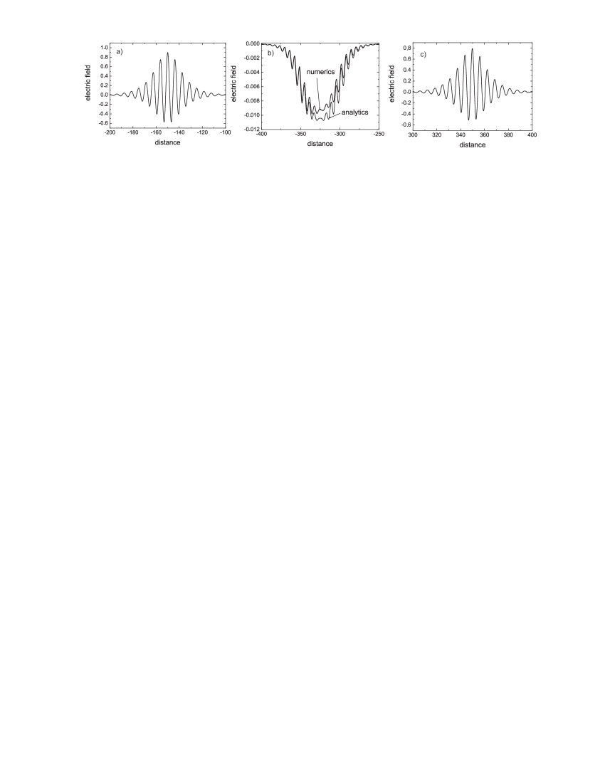
Figure 1: Snapshots of the electric field for the incident (a), reflected (b) and transmitted (c) pulses. Incident pulse given by Eq. (III) with $z_{0}=150$.

Let us turn now to consider the case of a conductive medium layer with a relatively thicker depth $L$ and higher static conductivity $\sigma_{0}$, so that $\sigma_{0}L/c$ is no longer a small parameter. Under these conditions, the validity of the analytical perturbation approach is no longer justified. In fact, this situation may be rather described by the approximate diffusion equation (10). Here we proceed with a comparison between the properties of solutions of the diffusion equation (10) for the magnetic field, with the numerical solutions of the Maxwell-Drude system of equations with initial conditions given as in Eq. (III) with $A_{1}=0$ (i.e., we only consider an input video-pulse).

In order to provide a better illustration of the diffusive dynamics of the field, we computed the spatial distributions of both electric and magnetic fields inside the conductive medium as time evolved. We found that the electric and magnetic field distributions appear to be qualitatively different. In fact, as a result of the flipping of the phase upon reflection from the boundary, the electric field develops negative regions in the vicinity of the boundary, which almost completely balance the positive regions situated farther from the boundary, so that $S_{E}^{(tr)}\equiv\int_{0}^{\infty}dz\,E(z,\,t)\approx 0$. As a consequence of this reflection dynamics, the value of the electric field at the boundary remains appreciably different from zero, and therefore the formula (17) is not directly applicable. More precisely, although the electric field eventually also exhibits a diffusive behavior, however such behavior is observed for relatively longer (when compared with the case of the magnetic field) observation times and also far from the boundary. In this respect, we would like to emphasize that although the diffusion equation (10) also correctly describes the evolution of the electric field at all times and everywhere inside the medium, because of its peculiar boundary conditions one may not simply apply to the electric field the analytically tractable model of a transparent boundary.

In contrast, it turns out that the diffusive behavior of the magnetic field is better predictable on the basis of the simple transparent boundary model. Indeed, the reflection of the magnetic field is not accompanied by a flipping of its phase, and as a consequence no negative field regions appear inside the conductive medium. Moreover, the magnetic field quickly approaches zero at the boundary. This leads to favorable conditions for the application of analytical formulas based on the distribution (17). First, in our numerical simulations we observed that the maximum of the magnetic field distribution indeed moves with time as $(t-t_{0})^{1/2}$. This means that the square of this quantity grows linearly with time, a behavior which is well supported by the plot in Fig. 2a that was obtained by the numerical integration of the Maxwell-Drude model. The slope of the straight line in Fig. 2a ($3.77$) is slightly different from the analytically predicted value of $4$. This discrepancy should be attributed to the difference in boundary conditions between the real case and the simple analytical model. We also plot in Fig. 2b the inverse of the square of the zeroth momentum (i.e. of the magnetic area of the transmitted pulse $S_{B}^{(tr)}=S_{0}^{(tr)}$). In support of the analytical predictions that are based on Eq. (17), again we observe an evolution described by a straight line immediately after that the incident pulse hits the boundary. From these observations we may conclude that the dynamics of the magnetic field inside the conductive medium is indeed of a diffusive nature.

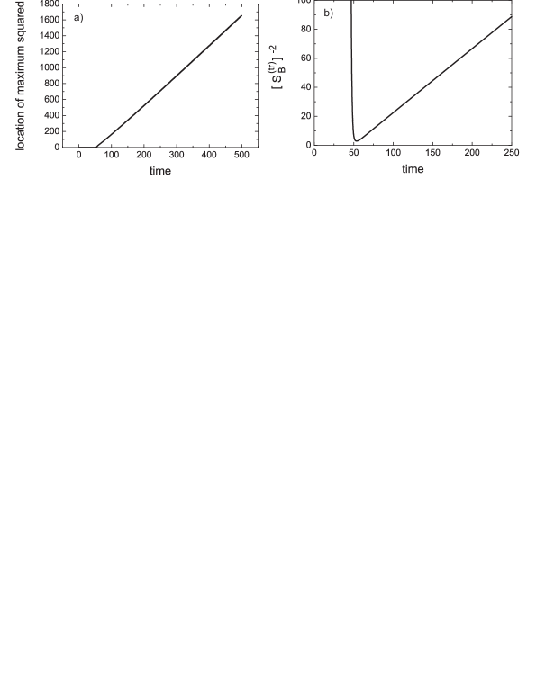
Figure 2: a) Location of the square of the maximum of the distribution of the magnetic field inside the medium as function of time; b) the inverse of $[S_{0}^{(tr)}]^{2}=[S_{B}^{(tr)}]^{2}$ as function of time. Parameters are $\nu=10$, $4\pi\sigma_{0}=0.5$.

IV The Maxwell-Drude-Bloch model

Let us include now in our model the presence of bound electronic states. This formally leads in the emergence of a medium polarization P, which is related to the electrical induction D via the well-known formula: ${\textbf{D}}={\textbf{E}}+4\pi{\textbf{P}}$. According to our model, the resonant component of the medium consists of a homogeneous mixture of two types of two-level doping centers, namely the absorbing (labeled by the index “p”, i.e. passive) and the amplifying (labelled by index “a”, i.e. active) centers. The total medium polarization in its scalar form is thus given by

$$P=N_{p}d_{p}\rho_{12}^{(p)}+N_{a}d_{a}\rho_{12}^{(a)}+{\textrm{c}.\textrm{c}.}$$ (36)

Here $N_{p,a}$ are the concentrations of passive and active two-level doping centers, $d_{p,a}$ are the (real) dipole matrix elements of transitions between upper (2) and lower (1) states, and $\rho_{mn}^{(p,a)}={\rho_{nm}^{(p,a)}}^{*}$ are the elements of the density matrix describing the resonant atom-like systems. For passive centers, the equations for the density matrix read as

$$\frac{\partial}{\partial t}\rho_{21}^{(p)}=-(i\omega_{21}^{(p)}+\gamma_{21}^{(p)})\rho_{21}^{(p)}-i\frac{d_{p}E}{\hbar}\,(\rho_{22}^{(p)}-\rho_{11}^{(p)})\,,$$ (37)

$$\frac{\partial}{\partial t}\rho_{22}^{(p)}=-\gamma_{2}^{(p)}\rho_{22}^{(p)}-i\frac{d_{p}E}{\hbar}\,(\rho_{21}^{(p)}-\rho_{12}^{(p)})\,,$$ (38)

$$\frac{\partial}{\partial t}\rho_{11}^{(p)}=\gamma_{2}^{(p)}\rho_{22}^{(p)}+i\frac{d_{p}E}{\hbar}\,(\rho_{21}^{(p)}-\rho_{12}^{(p)})\,.$$ (39)

Whereas for active centers one obtains

$$\frac{\partial}{\partial t}\rho_{21}^{(a)}=-(i\omega_{21}^{(a)}+\gamma_{21}^{(a)})\rho_{21}^{(a)}-i\frac{d_{a}E}{\hbar}\,(\rho_{22}^{(a)}-\rho_{11}^{(a)})\,,$$ (40)

$$\frac{\partial}{\partial t}\rho_{22}^{(a)}=-\gamma_{2}^{(a)}\rho_{22}^{(a)}-i\frac{d_{a}E}{\hbar}\,(\rho_{21}^{(a)}-\rho_{12}^{(a)})+p\,,$$ (41)

$$\frac{\partial}{\partial t}\rho_{11}^{(a)}=\gamma_{2}^{(a)}\rho_{22}^{(a)}-\gamma_{1}^{(a)}\rho_{11}^{(a)}+i\frac{d_{a}E}{\hbar}\,(\rho_{21}^{(a)}-\rho_{12}^{(a)})\,.$$ (42)

For simplicity, let us limit ourselves to consider atom-like doping centers with homogeneous broadening. In the above equations, $\omega_{21}^{(a,p)}$ are the transition frequencies, which are taken to be equal to each other, as well as to the carrier frequency $\omega_{0}$ of the incident femtosecond pulse; $\gamma_{21}^{(a,p)}$ are the polarization relaxation rates; $\gamma_{2}^{(a,p)}$ are the upper state population relaxation rates; $\gamma_{1}^{(a)}$ is population relaxation rate for the lower state of the active centers; and finally $p$ is the pump rate. As it follows from the above presented model equations, for passive centers one obtains a closed system where the lower state is the ground state. In contrast, the active two-level doping centers form an open system, since we supposed that there is a decay mechanism out of the two-level configuration, as well as pumping from some auxiliary upper level. Therefore we may only write the conservation law $\rho_{11}^{(p)}+\rho_{22}^{(p)}=1$ for passive centers; no such conservation holds the for the active doping two-level centers.

In our numerical simulations we used the following set of parameters: the ratio of dipole moments $\sqrt{\mu}=d_{p}/d_{a}$ was $1.5$, the relaxation rates were $\gamma_{1}^{(a)}=0.025$, $\gamma_{2}^{(a)}=0.005$, $\gamma_{2}^{(p)}=0.006$, $\gamma_{21}^{(p)}=0.0025$, $\gamma_{21}^{(a)}=0.015$, the pump rate was $p=0.004$. All of these quantities are expressed in units of the frequency $\omega_{0}$, so that the coupling constants between the field (or dimensionless Rabi frequency $\Omega=2d_{p}E/\hbar\omega_{21}^{(p)}$) and the polarizations induced by the passive and active centers read as $\beta=4\pi N_{p}d_{p}^{2}/\hbar\omega_{21}^{(p)}=0.1$ and $\kappa=4\pi N_{a}d_{p}d_{a}/\hbar\omega_{21}^{(a)}=0.02$.

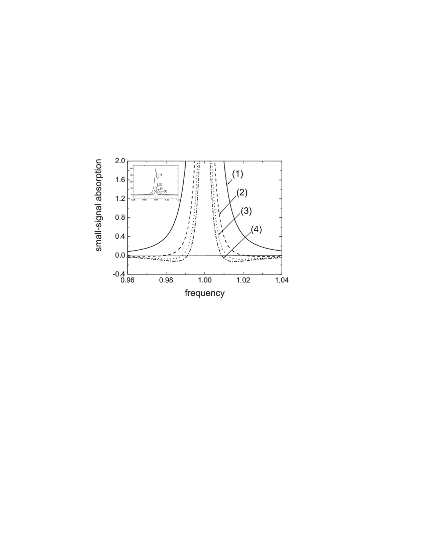
Figure 3: Small-signal absorption coefficient $\alpha(\omega)$ defined by Eq. (44) for four concentration levels of the passive centers $\beta$: (1) $0.1$; (2) $0.033$; (3) $0.014$; (4) $0.011$. Other parameters are as introduced in the text, moreover $\nu=10$ and $4\pi\sigma_{0}=0.005$. The curve (1) is everywhere positive, corresponding to the stability of the trivial solution. Full curves are shown in the inset.

From now on, we are going to solve in a self-consistent manner by the finite-difference time-domain method the coupled system including the wave equation (8), the Drude equation (22), and Bloch equations (37)-(42). Before describing the full numerical solutions of this Maxwell-Drude-Bloch (MDB) model, let us present the analytical stability analysis of its trivial solution ${\textbf{E}}=0$. Such analysis was described in a general form at the end of Section II. With a dispersion relation as in Eq. (21), we need to specify two ingredients, namely the frequency-dependent dielectric permittivity $\varepsilon(\omega)$ and the conductivity $\sigma(\omega)$. The latter is given in Eq. (24), whereas the former can be found from the linearized version of the density matrix equations (37)-(42). One obtains

$$\varepsilon(\omega)=1-\beta N_{eq}^{(p)}\frac{\omega+i\gamma_{21}^{(p)}}{\omega^{2}+{\gamma_{21}^{(p)}}^{2}}-\kappa\sqrt{\mu}N_{eq}^{(a)}\frac{\omega+i\gamma_{21}^{(a)}}{\omega^{2}+{\gamma_{21}^{(a)}}^{2}}\,.$$ (43)

Here $N_{eq}^{(p)}$ and $N_{eq}^{(a)}$ are the normalized equilibrium population differences of passive and active centers in the absence of electric field. For the above chosen parameters, one obtains $N_{eq}^{(p)}=-1$ and $N_{eq}^{(a)}=0.64$. By inserting Eqs. (24) and (43) in the dispersion relation Eq. (21), we may describe the propagation of a weak radiation in the conductive medium. For the trivial solution ${\textbf{E}}=0$ to be stable, radiation at all frequencies should decay upon propagation, so that the overall small-signal absorption coefficient

$$\alpha(\omega)=\mbox{sign \{Re}[k(\omega)]\}\,\mbox{Im}[k(\omega)]$$ (44)

must be non-negative for any positive value of $\omega$. A graphical representation of the frequency dependence of the small-gain absorption coefficient is given in Fig. 3. In this figure it is shown that, among the four curves shown here which correspond to different concentrations of the two-level absorbers, the stability condition is only satisfied for curve (1). Therefore, we used the corresponding concentration $\beta=0.1$ in our subsequent numerical simulations of the dissipative soliton generation. As it is usual for nonlinear dissipative systems, nonlinear gain may exceed nonlinear absorption, even though in the linear limit absorption prevails. The switching between the two regimes occurs due to the effect of a nonlinear (in our case, also coherent) bleaching of the absorption.

Given the above considerations, we are now ready to turn our attention to the full nonlinear problem. As it was previously discussed in VRS_06 , in a zero conductivity medium containing a purely resonant ensemble of amplifying and absorbing atom-like centers, few-cycle stationary pulses are metastable. In other words, for few-cycle pulses that propagate in such media there is a critical value of energy, such that pulses with lower (higher) energy eventually disperse (collapse). However, as we shall see in the following, in the presence of a nonzero and wideband conductivity as in the present MDB model, the pulse collapse effect may be suppressed. Indeed, we found that such stabilization of the pulse energy may take place for a wide range of variation of the collisional frequency $\nu$. We numerically checked the occurrence of the dissipative soliton energy stabilization process in the MDB model for three representative regimes, namely for $\nu=0.1$, $1$ and $10$ (in units of the carrier angular frequency $\omega_{0}$). As we are going to demonstrate a little later, the regime with $\nu\ll\omega_{0}$ turns out to be quantitatively closer to realistic semiconductor parameters. An example of numerically generated dissipative soliton within the MDB framework is illustrated in Fig. 4. The duration of this MDB soliton is less than two optical periods, and its spectrum (which is also shown in Fig. 4) is extremely wide (coherent supercontinuum). In fact the MDB soliton spectral width is comparable to the value of the transition frequency itself, and its spectrum is exactly centered at the transition frequency, in contrast with video-solitons (that were observed in a passive two-level scheme in Ref. BA_71 ) as well as the solitons that are formed in active-passive three-level ensembles of doping centers (see Refs. VRS_06 ; RSV_08 ). We did not observe generation of video-solitons in the MDB model. Physically, such property is associated with the high-pass filtering property of the conductive medium. Note that a similar situation was also observed in the dissipative soliton generation scheme which was presented in Ref. VRS_09 , where active and passive centers were embedded into a dielectric matrix that was characterized by an infra-red absorption band.

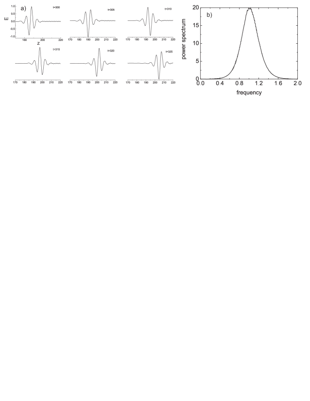
Figure 4: a) Profiles of the electric field (normalized Rabi frequency) of a few-cycle MDB dissipative soliton at different instants of time inside the conductive medium. The total tracking time covers approximately one period of the quasi-periodic motion of the soliton profile. b) The soliton spectrum. Specific parameters are $\nu=0.1$, $4\pi\sigma_{0}=0.005$.

The quasi-periodicity of the temporal profiles shown in Fig. 4 is related to the fact that the MDB soliton carrier frequency is distant from zero. If the soliton was propagating in vacuum, all of the snapshots which are shown in the figure would look exactly the same. However, whenever the soliton propagates in the conductive medium with both active and passive two-level doping centers, the soliton spatial profile varies in time. This is analogous to the case of the well-known self-induced transparency theory, where the propagation speed of the soliton envelope is different from the carrier phase velocity. A similar situation occurs in our case: we followed the zero-crossing of the field as it traverses through the (imaginary) pulse envelope, and we concluded with $1$% accuracy that their speed is equal to $c$, independently upon the precise location of a zero inside the envelope. In parallel, we also followed the speed of the motion of the soliton peak: for this particular case, we obtained a group speed of $0.69c$. Therefore we may indeed conclude that the carrier moves much faster than the (imaginary) pulse envelope.

Note that the weak ripples that modulate the spatial profiles (and correspondingly the spectrum) of the soliton pulse in Fig. 4 result from the initial transient process that leads to the formation, from the incident pulse, of a dissipative soliton inside the conductive medium. The input pulse that is incident from vacuum was set according to the expression in Eq. (III) with $A_{1}=0.75$. The profile of the soliton electric field which is illustrated in Fig. 4 is associated with corresponding spatial evolutions for the populations in both active and absorbing doping centers, as it is shown in Fig. 5. In particular, the evolution of the population difference among the two levels of the absorbing centers, as it is illustrated in Fig. 5b, reveals that almost complete inversion is achieved in the middle of the MDB soliton pulse. Whereas after the pulse the atomic-like systems return back to the ground state (except for a small tail which is the result of relaxation processes). Such behavior resembles the complete cycling of the population which is initiated by a $2\pi$-pulse of self-induced transparency in the theory of long optical pulses. In parallel, for the active centers the exchange among the populations of the upper and lower levels that is observed in the left side of Fig. 5 is analogous to the behavior of $\pi$-pulses, which have the property to invert the populations in a coherent amplifier. For relatively longer distances (not fully shown in the scale of the figure), the two-level populations of the active centers slowly restore their initial values as a result of the combined action of the relaxation and pumping processes.

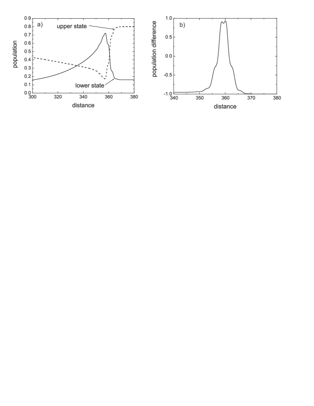
Figure 5: a) Spatial dynamics of the populations of the upper and lower states in the amplifying doping centers; b) spatial dynamics of the population difference in the absorbing centers. The parameters are the same as in Fig. 4, and the propagation time is $500$. Note the almost full inversion occurring at $z=357$ in the amplifiers.

V MDB soliton formation

The generation of MDB few-cycle solitons from an incident femtosecond pulse that we discussed in the previous section exhibits a threshold behavior, much in the same way as for other types of dissipative solitons. In other words, for a given set of medium parameters, a specific energy threshold exists for an incident pulse of a given shape: the dissipative soliton can only be formed whenever the incident pulse energy is larger than a specific threshold value. The existence of such an energy threshold is a direct consequence of the above discussed stability property of the trivial solution ${\textbf{E}}=0$. For the specific incident pulse shape that is given by Eq. (III), we may define a threshold value for the amplitude of the femtosecond pulse. Whenever $\nu=0.1$ and $4\pi\sigma_{0}=0.005$, such amplitude threshold is equal to $A_{1}=0.35$. Signals with smaller amplitudes are partly absorbed and partly reflected by the conductive medium. An example of pulse evolution in the case of an incident femtosecond pulse whose amplitude is below the threshold is shown in Fig. 6: we may notice from this figure that a remarkably large fraction of the incident optical pulse energy is back reflected at $t=300$. Such a strong reflection is due to resonantly-enhanced index of refraction of the two-level dopants of the medium. On the other hand, in the case of Fig. 6 the value of the conductivity and the interaction time are not large enough in order to cause a substantial reflection of the low-frequency electric field components. As a result, these components are virtually absent from the reflected pulse spectrum, which basically only includes high-frequency components, albeit slightly blue-shifted with respect to the resonance frequency. Figure 6 also shows that the resonant dispersion strongly affects the temporal shape of the reflected pulse. On the other hand, the transmitted pulse energy is relatively reduced with respect to the reflected counterpart. Indeed, Fig. 6 shows that the transmitted pulse is formed by the undistorted remainder of the incident video-pulse moving with speed close to $c$, with the addition of an high-frequency optical pulse whose irregular envelope travels with a group speed lower than $c$.

Figure 6: a) The incident pulse at $t=0$, and b) the pulse at $t=300$ in the linear regime of interaction. The vertical line indicates the boundary, arrows — the direction of propagation of the incident pulse. c) Spectra of the incident (solid), reflected (dashed) and transmitted (dotted) pulses. The parameters are: $\nu=10$, $4\pi\sigma_{0}=0.005$.

On the other hand, the evolution of an incident femtosecond pulse with an above-threshold amplitude results in the formation of a dissipative MDB soliton as discussed in the previous section (see also Fig. 4). The dynamics of such evolution is illustrated in Fig. 7: for this particular realization, the transient process leading to soliton formation from the incident pulse takes a few hundreds of dimensionless time units. The amplitude of the incident pulse, $A_{1}=0.75$, was chosen to be sufficiently large, so that in the vicinity of the boundary the optical frequency part of the transmitted pulse is separated into two sub-pulses that move with drastically different speeds. The fast-moving optical sub-pulse gradually transforms into a dissipative soliton; whereas its slowly-moving counterpart remains relatively close to the boundary, until eventually it dissipates away all of its energy. The gain which is provided by the active component of the medium is strongly depleted by the leading pulse, so that any subsequent pulse does not experience enough gain to compensate for its dissipative energy decay. In this sense, we may anticipate that the medium does not support the formation of multiple MDB solitons in the case of single pulse excitation: at least we did not detect such patterns in our simulations. Upon propagation in the conductive medium, the optical pulse energy in Fig. 7 slightly decreases, until a stationary value is reached. On the other hand, for relatively smaller values of the initial amplitude $A_{1}$ of the incident femtosecond pulse (still, with $A_{1}$ greater than $0.35$), we observed a growth of the pulse energy from its initial value up to a common asymptotic value. In contrast with the previously discussed linear regime of interaction with the medium, in the nonlinear case the fraction of incident optical pulse energy which is reflected from the boundary remains relatively small. In other words, we may say that at high power levels the boundary is virtually transparent, owing to the nonlinear saturation of the resonance of the two-level doping centers.

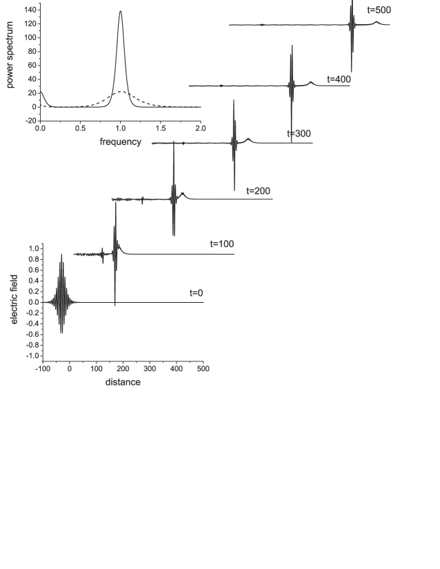
Figure 7: Evolution plots of the initial combination of a femtosecond pulse with $A_{1}=0.75$ and a video-pulse with $A_{0}=0.15$, showing soliton formation in a medium with parameters $\nu=10$ and $4\pi\sigma_{0}=0.005$. We also show the spectra of the incident (solid) and final (dashed) pulses.

Figure 7 also shows that the dissipative soliton generation process is accompanied by the propagation of a transient faster video pulse, or precursor, which gradually separates from the optical pulse as the field penetrates from the interface into the conductive medium. Indeed, such precursor results from the video pulse component of the incident field of Eq. (III), and it propagates with speed close to $c$. As a matter of fact, at low frequencies the electric field is out of resonance with the two-level doping centers, hence it is not subject to the slowing down which caused by the resonance mechanism. Nevertheless, the transmitted video pulse decays exponentially in time, as it transfers its energy to free electrons via the Drude conductivity. In summary, we found that the ultimate shape of the few cycle optical soliton is virtually independent upon the precise details of the input field excitation process. In particular, the MDB soliton shape does not depend on the presence or absence of input video-pulse: exactly the same few-cycle optical soliton could be generated with $A_{0}=0$. Moreover, the profiles of the MDB soliton electric and magnetic fields are almost indistinguishable. In Fig. 7 we also compare the spectra of the incident and the transmitted pulses: here the spectrum of the transmitted pulse coincides with the soliton spectrum that was earlier illustrated in Fig. 4. Note the substantial spectral broadening of soliton spectrum with respect to the spectrum of the incident femtosecond pulse, thanks to the effect of temporal compression that has been induced by the medium.

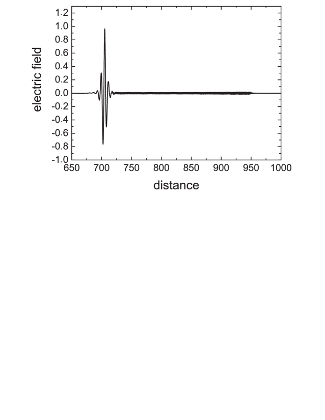
Figure 8: The shape of the pulse after $1000$ time units of propagation in the conductive medium with $\nu=0.1$ and $4\pi\sigma_{0}=0.005$. Note that the precursor is spread out over large distance, while the soliton preserves the shape found in other simulations.

We also performed additional simulations with $\nu=1$ and $\nu=0.1$, while keeping unchanged the value of the conductivity at the resonance frequency. In all of these cases we obtained evolution plots for the electric field which do not differ much from that shown in Fig. 7, so that it would be redundant to present them all. Instead, we plot in Fig. 8 the final temporal profile of the MDB soliton pulse after $1000$ time units of propagation in the conductive medium with $\nu=0.1$ and $4\pi\sigma_{0}=0.005$. The only visible difference with respect to the final MDB soliton profile that was shown in Fig. 7 is the relatively much larger spreading of the precursor: instead of the compact, bell-type shaped video pulse of Fig. 7, we obtained a low-amplitude precursor with a modulation frequency $3.5$ times larger than the resonance frequency. In this case the breakdown of the input video-pulse may be attributed to the prevalence of the derivative term over the collisional term in the Drude equation (22).

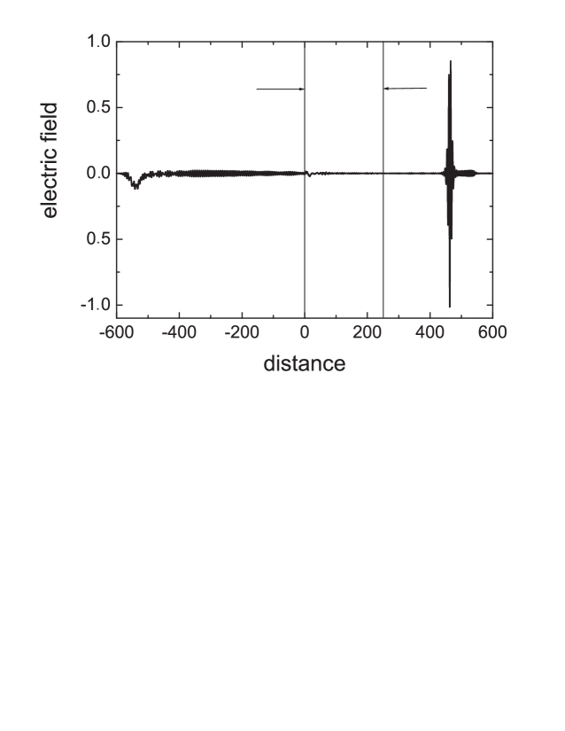
Figure 9: Pulse from a finite layer of the medium: a soliton and a precursor are formed. The parameters are $\nu=0.1$ and $4\pi\sigma_{0}=0.005$. Boundaries are indicated by thin vertical lines.

Before concluding the description of the evolution of the electromagnetic field within the framework of the Maxwell-Drude-Bloch model, we show in Fig. 9 the case of a pulse passing through a thick but finite layer of the conductive medium. The inclusion of a second (or output) interface brings our model closer to a real experiment. The layer was set to be thick enough ($z=250$) in order to allow for completing the formation of the dissipative MDB soliton from the incident pulse. The plot in Fig. 9 aims at demonstrating the absence of dramatic changes to the soliton shape when passing from the medium through the boundary to vacuum. However in this case the medium thickness was not enough to fully dissipate the incident video-pulse. As a result, a precursor still accompanies the MDB soliton. Note that the presence of such a precursor is somewhat artificial. In fact, we included in the incident pulse a video-pulse component in order to be able of following the evolution of low-frequency radiation in the conductive medium. Clearly in practical experimental conditions an incident femtosecond pulse is sufficient for the excitation of a MDB soliton: in this case no precursor would be observed, apart from possible radiation initiated in the transient process.

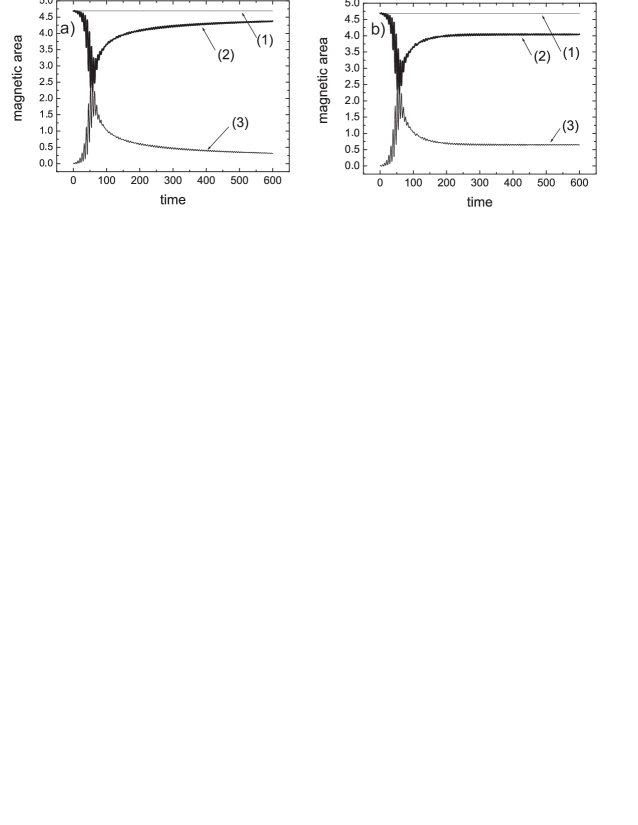
Figure 10: Total magnetic area (1), the magnetic area of the reflected (2) and transmitted (3) pulses for thick, $L=250$, (a) and thin, $L=25$, (b) layers. Parameters are $\nu=0.1$ and $4\pi\sigma_{0}=0.005$.

Finally, let us turn our attention to the discussion of the dynamics of the evolution of low-frequency pulse components, or video-pulse. The conductive component of the medium plays here the dominant role, whereas the resonant atom-like systems have a negligible influence. As we shall see, the notion of magnetic area lies at the heart of this discussion. Let us consider the total magnetic area as defined according to Eq. (4), and the partial areas

$$S_{B}^{(tr)}(t)=\int_{0}^{\infty}dz\,B(z,t)\quad\mbox{and}\quad S_{B}^{(ref)}(t)=\int_{-\infty}^{0}dz\,B(z,t)$$ (45)

for the transmitted and reflected pulses, respectively. Clearly, the sum of the last two areas yields the total magnetic area. Let us recall here that the area of the magnetic field equals its zero-frequency Fourier component.

Let us examine the two limit cases of a pulse crossing either a thick or a thin layer of conductive medium. Figure 10 shows the corresponding time evolutions of the magnetic area. The total magnetic area is a conserved quantity in both cases, a conclusion that follows from the analytical formula (5) and which is well confirmed by the computer-generated plots of Fig. 10. As it can be seen from Fig. 10, in the case of a thin medium the two partial magnetic areas reach their corresponding asymptotic values in a relatively short time. On the other hand, for a thick layer the magnetic areas of the reflected and the transmitted pulses do not reach their asymptotic values within the total time of observation. Such slow time evolution of the magnetic area reflects the continuous creation of evanescent waves inside the medium. Such evanescent field is associated with the nearly unitary reflection coefficient at zero frequencies. As a result, one obtains a relatively long decay time of the partial magnetic areas. It is remarkable that the evanescent field, which appears as a long, non-oscillating and slowly decaying tail that follows the main pulse, is not even visible on the scale of previous plots such as Fig. 9. The reason is that this tail is of vanishing intensity, thus it contributes a relatively small fraction to the total energy of the pulse. Nevertheless, the electric area of the tail may remain quite substantial, as it is proportional to the tail amplitude multiplied by its long spatial extension. wave.

In the case of a thin layer of the medium, Fig. 10 shows that the asymptotic values of the partial magnetic areas are readily achievable within a relatively short observation time. This corresponds to the fact that here the reflection coefficient is noticeably different from unity at zero frequencies (frustrated total internal reflection). In other words, the evanescent wave simply tunnels through the thin layer of conductive material, and carries the energy of low-frequency components through the layer. In summary, the analysis of the temporal dynamics of the magnetic area permits us to investigate the details of the propagation of evanescent waves through a finite conductive medium.

VI Discussion

In this work we studied the linear and nonlinear dynamics of the propagation of broadband radiation which is incident on the interface with a conductive medium, doped with active and passive two-level atom-like systems. To this end, we introduced the Maxwell-Drude-Bloch model, which appears as a promising approach for the description of actual devices in modern nonlinear optics. In fact, the MDB model allows for the consideration of the full Lorentz model of matter, which accounts for the interaction of light with both free as well as bound electrons. We anticipate that the dynamics of free charges may become particularly important when describing doped semiconductor materials. An appropriate generalization of the model which was presented here will include of the nonlinear response of the electric current, which is typical of photovoltaic phenomena.

We have shown that, within the framework of the Maxwell-Drude-Bloch model, stable few-cycle dissipative solitons can be formed. A remarkable feature of the present scheme is that these MDB solitons may be excited by a relatively long (albeit rather powerful) femtosecond pulse which is incident from vacuum onto the boundary with the conductive medium, doped with passive and active atom-like systems. It is important to note that the process of pulse compression leading to soliton formation is not energy-consuming: quite to the opposite, soliton generation may even be accompanied by a power increase, thanks to the presence of gain in the medium. The dissipative solitons can be only excited by rather powerful pulses, with energies exceeding certain threshold (hard excitation). These few-cycle MDB solitons are characterized by a wide spectrum (coherent supercontinuum), whose carrier is centered at the resonance frequency. On the other hand, given low transmissivity of the conductive medium at low frequencies, we do not expect the formation of video-solitons by the present scheme.

The process of formation of few-cycle solitons involves the rather natural assumption that the initial pulse is incident from vacuum on the boundary with the conductive doped medium. In this case, one must properly take into account the high reflectivity of such a medium at low frequencies. As a matter of fact, the medium is totally reflective at zero frequency only, and in the case of both a semi-infinite medium and an indefinitely long interaction time. On the other hand, in the case of propagation through a thin layer of the medium, one only obtains a partial reflection of low frequency waves, owing to the tunneling of evanescent waves. As a consequence, in this case instead of total reflection one observes a long and low-intensity tail of radiation that follows the transmitted main optical pulse. Even though such a tail carries a relatively small fraction of energy, its area may remain quite substantial. In order to characterize these low-frequency tails, we introduced the notion of temporal magnetic area, see Eq. 4. For this quantity we found a conservation law in the form of Eq. (5), which holds well beyond the framework of the Maxwell-Drude-Bloch model, that is for virtually any pulsed electromagnetic radiation that propagates in a homogeneous or inhomogeneous medium with free and bound charges and dissipation. We also found it quite instructive to separate the total magnetic area in two parts – namely, the transmitted and reflected areas, as these quantities characterize the low-frequency tails of the transmitted and reflected pulses, respectively.

For low-frequency pulses, we have derived a parabolic equation (10), that describes the process of diffusion of the electromagnetic field in a highly conductive medium. Though the parabolic equation has been known in the electromagnetics of quasi-stationary fields, LL ; Jackson , here we reveal its new application to video-pulses and demonstrate the propagation dynamics of these pulses and related evolution of their magnetic area. This equation may be also useful in studies involving the propagation of THz radiation in high conductivity materials.

In the end, let us present some numerical estimates for the effective values of the conductivity and the collisional frequency. The latter can be found if the mobility $\mu=e/\nu m_{\mbox{eff}}$ and the effective mass $m_{\mbox{eff}}$ of the carriers are known. For GaAs we get $\mu=0.85$ m²/$(V\cdot s)$ and $m_{\mbox{eff}}=0.067m_{e}$, so that $\nu\approx 3\cdot 10^{12}$ Hz; for AlAs: $\mu=0.028$ m²/$(V\cdot s)$, $m_{\mbox{eff}}=0.1m_{e}$ and $\nu\approx 6\cdot 10^{13}$ Hz, semi1 ; semi2 . Both values of the collisional frequency $\nu$ are much smaller than the optical frequency ($\omega_{0}\sim 5\cdot 10^{14}$ Hz), which corresponds to the limit case $\nu\ll\omega_{0}$. For infrared radiation one may obtain an intermediate situation $\nu\simeq\omega_{0}$, whereas for THz radiation this inequality is reversed, namely $\omega_{0}\ll\nu$. In all of these cases we observed the stable generation of dissipative MDB solitons.

Another important estimate involves the value of the static conductivity, which is usually measured in SI units. Therefore we rewrite the expression for the quantity $4\pi\sigma_{0}$ (which is normalized with respect to the optical frequency $\omega_{0}$) that we have used throughout our simulations, as

$$4\pi\sigma_{0}=\frac{c^{2}\mu_{0}}{\omega_{0}}\,\frac{1}{2}N_{e}e\mu$$ (46)

where we used Eq. (23) expressed in CGSE units, and rewritten here in terms of the mobility parameter; $\mu_{0}=1.257\cdot 10^{-6}$ H/m is the magnetic permeability of the vacuum. For $\mu=0.85$ m²/$(V\cdot s)$ and $\omega_{0}\sim 5\cdot 10^{14}$ Hz, we get the estimate

$$4\pi\sigma_{0}=1.3\cdot 10^{-23}N_{e}(\mbox{m}^{-3})\,.$$ (47)

For the value of $4\pi\sigma_{0}=0.005$ that we used in the above simulations for demonstrating the generation of dissipative solitons, the concentration of free carriers is $N_{e}=3\cdot 10^{14}$ cm^-3 (this is approximately equal to the concentration of dopants in the host semiconductor material). Such value of dopant concentration is rather modest. Clearly for higher values of the concentration the conductivity would be even more significant.

In order to implement the two-level gain and absorbing doping centers, we may suggest the use quantum dots, i.e. the same medium as in the scheme with three-level atomic-like doping centers that was proposed in Ref. VRS_09 . However in the present situation the quantum dots would not be embedded in quartz as in Ref. VRS_09 , but in a semiconductor environment. Due to their huge dipole moments, the use of quantum dots may permit a decrease by several orders of magnitude of the peak intensities of the electromagnetic radiation, thereby avoiding the occurrence of a nonlinear response or even breakdown of the host matrix. Some associated numerical estimates can be found in Ref. VRS_09 . Note that for the specific values, that we used in our simulations, of quantum dot concentrations of the order of $10^{18}$ cm^-3, the thickness of the medium which is necessary for the development of a dissipative soliton is less than one millimeter. These rather high concentration levels, as well as the relatively fast decay constants into the asymptotic soliton solution are not crucial to our scheme, and merely served for permitting a fast numerical convergence of the initial pulse into the soliton. Therefore the doping concentration could be reduced by an order of magnitude without preventing the applicability of our scheme, but possibly at the expense of device miniaturization.

The broadband losses that are introduced by the conductivity represent the main stabilization mechanism of the dissipative solitons. We anticipate that in a laser where the active two-level systems play the role of a gain medium, passive two-level absorbers would play the role of a mode-locker in a passive mode-locking configuration, whereas the role of the broadband losses may be taken by the outcoupling mirror as in the coherent mode-locking technique that was proposed in Ref. kozlov . In conclusion, we may anticipate that few-cycle dissipative solitons may be also generated in a laser cavity configuration: such a scheme is reserved for future investigation and will be published elsewhere.

Appendix A Derivation of equations (29) and (30)

In the first order of the perturbation theory, the wave equation (8) takes the form

$$\frac{\partial^{2}E_{1}}{\partial\xi\partial\eta}=-\frac{\pi\sigma_{0}}{c}\,\frac{\partial A}{\partial\xi}$$ (48)

where $\eta=z+ct$ and $\xi=z-ct$. The general solution of this equation reads

$$E_{1}(\xi,\,\eta)=-\frac{\pi\sigma_{0}}{c}\,E_{f}(\xi)\eta+F(\xi)+B(\eta)\,,$$ (49)

where $F$ and $B$ are arbitrary functions of their variables. In terms of the original variables we have

$$E_{1}(z,\,t)=-\frac{\pi\sigma_{0}}{c}\,E_{f}(z-ct)(z+ct)+F(z-ct)+B(z+ct)\,.$$ (50)

The first terms in Eqs. (49) and (50) in the right-hand sides represent a particular solution of inhomogeneous equation (48), the second and third terms represent forward ($F$) and backward ($B$) travelling waves, respectively. Finally, the field $E(z,\,t)$ acquires the form

$$E(z,t)=\left\{\begin{array}[]{l}E_{f}(z-\tau)+E_{b}(z+\tau)\quad\mbox{for}\,z<0\,,\\ \left[1-\frac{\pi\sigma_{0}}{c}(z+\tau)\right]E_{f}(z-\tau)+F(z-\tau)+B(z+\tau)\quad\mbox{for}\,0<z<L\,,\\ E_{tr}(z-\tau)\quad\mbox{for}\,z>L\,.\end{array}\right.$$ (51)

Here $\tau=ct$ and $E_{f}$ is given function – the shape of the incident pulse. Unknown functions are $E_{f}$, $F$, $B$, and $E_{tr}$; each of them is a function of a single variable. The unknown functions are to be found from the continuity conditions of $E$ and $\partial E/\partial z$ at $z=0$ and $z=L$:

$$E_{b}(\tau)=-\frac{\pi\sigma_{0}}{c}\,\tau E_{f}(-\tau)+F(-\tau)+B(\tau)\,,$$

$$E_{b}^{\prime}(\tau)=-\frac{\pi\sigma_{0}}{c}\left[E_{f}(-\tau)+\tau E^{\prime}_{f}(-\tau)\right]+F^{\prime}(-\tau)+B^{\prime}(\tau)\,,$$ (52)

$$\left[1-\frac{\pi\sigma_{0}}{c}(L+\tau)\right]E_{f}(L-\tau)+F(L-\tau)+B(L+\tau)=E_{tr}(L-\tau)\,,$$

$$\left[1-\frac{\pi\sigma_{0}}{c}(L+\tau)\right]E_{f}^{\prime}(L-\tau)-\frac{\pi\sigma_{0}}{c}\,E_{f}(L-\tau)+F^{\prime}(L-\tau)+B^{\prime}(L+\tau)=E^{\prime}_{tr}(L-\tau)\,.$$

The prime indicates the differentiation of the corresponding function with respect to $\tau$. Let us rewrite the set of equations (52) after differentiating the first and the third equations with respect to $\tau$:

$$E^{\prime}_{b}(\tau)=-\frac{\pi\sigma_{0}}{c}\left[E_{f}(-\tau)-\tau E^{\prime}_{f}(-\tau)\right]-F^{\prime}(-\tau)+B^{\prime}(\tau)\,,$$

$$E_{b}^{\prime}(\tau)=-\frac{\pi\sigma_{0}}{c}\left[E_{f}(-\tau)+\tau E^{\prime}_{f}(-\tau)\right]+F^{\prime}(-\tau)+B^{\prime}(\tau)\,,$$ (53)

$$-\frac{\pi\sigma_{0}}{c}\,E_{f}(L-\tau)-\left[1-\frac{\pi\sigma_{0}}{c}(L+\tau)\right]E^{\prime}_{f}(L-\tau)-F^{\prime}(L-\tau)+B^{\prime}(L+\tau)=-E^{\prime}_{tr}(L-\tau)\,,$$

$$-\frac{\pi\sigma_{0}}{c}\,E_{f}(L-\tau)+\left[1-\frac{\pi\sigma_{0}}{c}(L+\tau)\right]E_{f}^{\prime}(L-\tau)+F^{\prime}(L-\tau)+B^{\prime}(L+\tau)=E^{\prime}_{tr}(L-\tau)\,.$$

Subtracting the second equation from the first we get

$$F^{\prime}(-\tau)=\frac{\pi\sigma_{0}}{c}\,\tau\,E_{f}^{\prime}(-\tau)\,,$$ (54)

and therefore

$$F(\tau)=-\frac{\pi\sigma_{0}}{c}\,\int_{-\infty}^{\tau}d\theta\,\theta\,E_{f}^{\prime}(\theta)\,.$$ (55)

Summing up these two equations we find

$$E^{\prime}_{b}(\tau)=-\frac{\pi\sigma_{0}}{c}\,E_{f}(-\tau)+B^{\prime}(\tau)\,.$$ (56)

Similar manipulations are to be performed with last two equations in (53). Summation yields

$$B^{\prime}(L+\tau)=\frac{\pi\sigma_{0}}{c}\,E_{f}(L-\tau)\,.$$ (57)

From this result we find

$$B^{\prime}(\tau)=\frac{\pi\sigma_{0}}{c}\,E_{f}(2L-\tau)$$ (58)

and

$$B(\tau)=\frac{\pi\sigma_{0}}{c}\,\int_{-\infty}^{\tau}d\theta\,E_{f}(2L-\theta)\,.$$ (59)

Combining equations (56) and (58), we obtain the shape of the reflected pulse, see Eq. (30).

Finally, by subtracting last two equations in the system (53) from each other we get

$$E^{\prime}_{tr}(L-\tau)=\left[1-\frac{\pi\sigma_{0}}{c}(L+\tau)\right]\,E^{\prime}_{f}(L-\tau)+F^{\prime}(L-\tau)$$ (60)

and therefore

$$E^{\prime}_{tr}(\tau)=\left[1-\frac{\pi\sigma_{0}}{c}(2L-\tau)\right]\,E^{\prime}_{f}(\tau)+F^{\prime}(\tau)=\left[1-\frac{\pi\sigma_{0}}{c}\,L\right]\,E_{f}^{\prime}(\tau)\,.$$ (61)

Integration of the last formula gives Eq. (29).