Near term measurements with 21 cm intensity mapping: neutral hydrogen fraction and BAO at $z<2$

Abstract

It is shown that 21 cm intensity mapping could be used in the near term to make cosmologically useful measurements. Large scale structure could be detected using existing radio telescopes, or using prototypes for dedicated redshift survey telescopes. This would provide a measure of the mean neutral hydrogen density, using redshift space distortions to break the degeneracy with the linear bias. We find that with only 200 hours of observing time on the Green Bank Telescope, the neutral hydrogen density could be measured to 25% precision at redshift $0.54<z<1.09$. This compares favourably to current measurements, uses independent techniques, and would settle the controversy over an important parameter which impacts galaxy formation studies. In addition, a 4000 hour survey would allow for the detection of baryon acoustic oscillations, giving a cosmological distance measure at 3.5% precision. These observation time requirements could be greatly reduced with the construction of multiple pixel receivers. Similar results are possible using prototypes for dedicated cylindrical telescopes on month time scales, or SKA pathfinder aperture arrays on day time scales. Such measurements promise to improve our understanding of these quantities while beating a path for future generations of hydrogen surveys.

I Introduction

An upcoming class of experiments propose the observation of the 21 cm spectral line over large volumes, detecting large scale structure in three dimensions Peterson et al. (2009). This method is sensitive to a redshift range of $z\gtrsim 1$, which is observationally difficult for optical experiments, due to a dearth of spectral lines in the atmospheric transparency window. Such experiments require only limited resolution to resolve the structures of primary cosmological interest, above the non-linear scale. At $z\approx 1$ this corresponds to tenths of degrees. There is no need to detect individual galaxies, and in general each pixel will contain many. This process is referred to as 21 cm intensity mapping. A first detection of large scale structure in the 21 cm intensity field was reported in 2008 Pen et al. (2008).

Intensity mapping is sensitive to the large scale power spectra in both the transverse and longitudinal directions. From this signal, signatures such as the baryon acoustic oscillations (BAO), weak lensing and redshift space distortions (RSD) can be detected and used to gain cosmological insight.

To perform such a survey dedicated cylindrical radio telescopes have been proposed Peterson et al. (2006); Seo et al. (2009), which could map a large fraction of the sky over a wide redshift range and on timescales of several years. These experiments are economical since their low resolution requirements imply limited size and they have no moving parts. It has been shown that BAO detections from 21 cm intensity mapping are powerful probes of dark energy, comparing favourably with Dark Energy Task Force Stage IV projects within the figure of merit framework Chang et al. (2008); Albrecht et al. (2006). Additionally, in Masui et al. (2010) it was shown that such experiments could tightly constrain theories of modified gravity, making extensive use of weak lensing information. The $f(R)$ theory, for instance, could be constrained nearly to the point where the chameleon mechanism masks any deviations from standard gravity before they first appear.

While such experiments will be very powerful probes of the Universe, it is useful to explore how 21 cm intensity mapping could be employed in the short term. Here we discuss surveys that could be performed using existing radio telescopes, where the Green Bank Telescope will be used as an example. Prototypes for the above mentioned cylindrical telescopes (for which some infrastructure already exists) are also considered. Finally, the Square Kilometre Array Design Studies (SKADS) focused on developing aperture array technology for the Square Kilometre Array Faulkner et al. (2010). Motivated by the proposed Aperture Array Astronomical Imaging Verification (A3IV) project van Ardenne (2009); aav , we consider pathfinders for such arrays. These aperture arrays could share many characteristics in common with cylindrical telescope prototypes, but would be capable of much greater survey speed.

While these limited resources would not have nearly the statistical power required to detect effects like weak lensing, a detection of the RSD would be possible. This would give a measure of the mean density of neutral hydrogen in the Universe. This has been an important and controversial parameter in galaxy formation studies and a precise measurement would be invaluable in this field Putman et al. (2009). In addition BAO are considered, a detection of which would yield cosmologically useful information about the Universe’s expansion history.

In this paper we first describe the RSD and BAO and the information that can be achieved with their detection. We then present forecasts for 21 cm redshift surveys as a function of telescope time, followed by a brief discussion of these results.

We assume a fiducial $\Lambda\mathrm{CDM}$ cosmology with parameters: $\Omega_{m}=0.24$, $\Omega_{b}=0.042$, $\Omega_{\Lambda}=0.76$, $h=0.73$, $n_{s}=0.95$ and $\log_{10}A_{s}=-8.64$; where these represent the matter, baryon and vacuum energy densities (as fractions of the critical density), the dimensionless Hubble constant, spectral index and logarithm of the amplitude of scalar perturbations.

II Redshift Space Distortions

In spectroscopic surveys, radial distances are given by redshifts. However redshift does not map directly onto distance as matter also has peculiar velocities, which Doppler shifts incoming photons. On large scales, these velocities are coherent and result in additional apparent clustering of matter in redshift space. In linear theory, the net effect is an enhancement of power for Fourier modes with wave vectors along the line of sight Kaiser (1987),

$$P^{\rm s}_{X}(\vec{k},z)=b^{2}\left[1+\beta(z)\mu_{\hat{k}}^{2}\right]^{2}P(k,z).$$ (1)

Here $P^{s}_{X}$ is the power spectrum of tracer $X$ (assumed to be linearly biased) as observed in redshift space, $P$ is the matter power spectrum and $\mu_{\hat{k}}=\hat{k}\cdot\hat{z}$. The bias, $b$, quantifies the degree to which the density perturbation of the tracer follows the density perturbation of the underlying dark matter. The redshift space distortion parameter $\beta$ is equal to $f/b$ in linear theory, where $f$ is the dimensionless linear growth rate. To a good approximation $f(z)=\Omega_{m}(z)^{0.55}$.

We define the signal neutral hydrogen power spectrum as

$$\tilde{P}_{\rm HI}(\vec{k},z)\equiv x_{\rm HI}^{2}P^{\rm s}_{\rm HI}(\vec{k},z),$$ (2)

where $x_{\rm HI}(z)$ is the mean fraction of hydrogen that is neutral. It is the parameter $x_{\rm HI}$ that we wish to measure. The above definition is useful because it defines the quantity that is most directly measured in a 21 cm redshift survey. Note that in discussions of the more standard galaxy redshift surveys one usually takes a measurement of the mean density for granted; however, 21 cm intensity mapping will make differential measurements and will not measure the mean signal directly. One cannot divide out the mean to define a measurement of fluctuations around the mean. Using the fact that at late times, on large scales, structure undergoes scale independent growth, the above quantity can be written as

$$\tilde{P}_{\rm HI}(\vec{k},z)=b^{2}x_{\rm HI}^{2}\left(\frac{g(z)a}{a_{0}}\right)^{2}\left[1+\beta\mu_{\hat{k}}^{2}\right]^{2}P(k,z_{0}),$$ (3)

where subscript $0$ refers to some early time well after recombination and $g$ is the growth factor (relative to an Einstein-de Sitter Universe).

Because the power spectrum at early times, $P(k,z_{0})$, can be inferred from the Cosmic Microwave Background (to good enough accuracy for our purposes in this paper), the observed power spectrum can be parameterized by just two redshift dependent numbers, $\beta$ and the combination of scale independent prefactors in Equation 3,

$$A_{H}\equiv b^{2}x_{\rm HI}^{2}g^{2}.$$ (4)

It is these two parameters that can be determined from a 21 cm redshift survey using the RSD. In general $A_{H}$ will be better measured than $\beta$ and does not significantly contribute to the uncertainty in $x_{\rm HI}$.

The factors $f(z)$ and $g(z)$ depend on the expansion history. If one allows for a general expansion history (for instance, the WMAP allowed CDM model with arbitrary curvature and equation of state, OWCDM) these factors are poorly determined since there is currently little data that directly probes the expansion in this era. However, if one is willing to assume a flat $\Lambda\mathrm{CDM}$ expansion history, then the current uncertainty in the late time expansion is attenuated at the redshifts of interest (since dark energy is sub-dominant to matter at $z=1$) and uncertainties in theses parameters can be ignored.

As such, a measurement of $\beta$ gives a measurement of the bias $b$ which in turn gives a measurement of $x_{HI}$. We have

$$\frac{\Delta x_{\rm HI}}{x_{\rm HI}}\approx\frac{\Delta\beta}{\beta}\qquad\text{($\Lambda\mathrm{CDM}${} assumed)}.$$ (5)

If one is not willing to assume an expansion history, it is a simple matter to propagate the corresponding uncertainties in the expansion parameters.

To estimate errors on $\beta$, we assume that the primordial power spectrum is essentially known from the cosmic microwave background, and we fix all parameters except for the amplitude $A_{s}$, spectral index $n_{s}$, and running of the spectral index $\alpha_{s}$. The observable power spectrum is then parameterized by $\beta$, $A_{s}$, $n_{s}$ and $\alpha_{s}$. We then use the Fisher matrix formalism to determine how precisely $\beta$ can be measured from the 21 cm survey, marginalizing over the other three parameters and using no other information. The parameter $A_{s}$ is used as a stand-in for the other parameters that affect the overall amplitude of the power spectrum: the bias and $x_{\rm HI}$. Its marginalization is critical to account for the fact that we have no a priori information about these parameters. The spectral index marginalization is not strictly necessary but allows for some degradation due to concern about scale dependence of bias. We have restricted the numerator of the Fisher matrix to include only the linear theory power as suppressed by the non-linear BAO erasure kernels of Seo and Eisenstein (2007) (all the linear power is included though, not BAO only), so non-linearity should not be a significant issue at the level of precision discussed here. This treatment of the non-linearity cutoff is also motivated by the propagator work of Crocce and Scoccimarro (2006a, b, 2008).

III Baryon Acoustic Oscillations

Acoustic oscillations in the primordial photon-baryon plasma have ubiquitously left a distinctive imprint in the distribution of matter in the Universe today. This process is understood from first principles and gives a clean length scale in the Universe’s large scale structure, largely free of systematic uncertainties, and calibrations. This can be used to measure the global cosmological expansion history through the angular diameter distance vs redshift relation. The detailed expansion will differ between a pure cosmological constant and the various other cosmological models.

We use essentially the method of Seo and Eisenstein (2007) for estimating distance errors obtainable from a BAO measurement, including 50% reconstruction of nonlinear degradation of the BAO feature (although this is unimportant since experiments considered here have low resolution). The BAO feature is isolated by dividing the total power spectrum Eisenstein and Hu (1998) by the wiggle-free power spectrum and subtracting unity, as illustrated in Figure 1. The wiggles are then parameterized by an overall amplitude, and a length scale dilation (here $A_{w}$ and $D$ respectively), which control the vertical and horizontal stretch of the theoretical curve shown in Figure 1. Our errors on $A_{w}$ come from a straightforward extension of the Seo and Eisenstein (2007) method for estimating BAO errors. In addition to the BAO distance scale as a free parameter in our Fisher matrix, we include $A_{w}$ as a free parameter. This is similar to what one sometimes tries to do by including the baryon/dark matter density ratio as a parameter, but more straightforward to interpret.

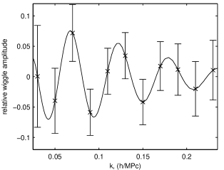
Figure 1: Baryon acoustic oscillations averaged over all directions. To show the BAO we plot the ratio of the full matter power spectrum to the wiggle-free power spectrum of Eisenstein and Hu (1998). The error bars represent projections of the sensitivity possible with 4000 hours observing time on GBT at $0.54<z<1.09$.

The ability to measure $A_{w}$ (which is zero in the absence of the BAO) represents the ability to detect the presence these wiggles. A measurement of $D$ allows one to associate a comoving distance to length scales on the sky. This gives a measurement of the angular diameter distance ($d_{A}$) for detections in the transverse direction, and the Hubble parameter ($H$) if the wiggles are detected in the longitudinal direction.

IV Forecasts

We present forecasts for the Green Bank Telescope and prototypes for two classes of telescope: cylindrical telescopes and SKA aperture arrays. The signal available for 21 cm experiments is proportional to the neutral hydrogen fraction and bias. For estimating telescope sensitivity we assume that the product of the bias and the neutral hydrogen density $\Omega_{\rm HI}b=0.0004$ todayChang et al. (2008), and that the neutral hydrogen fraction and bias do not evolve. These assumptions only affect the sensitivity of the telescopes and not the translation from uncertainty on $P^{s}_{\rm HI}$ to the uncertainty on $x_{\rm HI}$. Also, as in galaxy surveys, there is expected to stochastic shot noise component and we assume Poisson noise with an effective object number density $\bar{n}=0.03$ per cubic $h^{-1}\rm{Mpc}$. Note that stochastic noise at this level is negligible, as should be the case in practice.

The 21 cm intensity mapping technique is expected to be complicated by a variety of contaminating effects. These include diffuse foregrounds (predominantly galactic synchrotron), radio frequency interference and bright point sources. The degree to which these contaminants will limit future surveys has yet to be quantified, and here we simply ignore them. As such these forecasts are theoretical idealizations. Methods for dealing with these contaminants are discussed in Chang et al. (2008).

The Green Bank Telescope is a 100 m diameter circular telescope with a system temperature of 25 K. It has interchangeable single pixel receivers at the frequencies of interest with bandwidths of approximately 200 MHz. For extended surveys, multiple pixel receivers could be implemented. The construction of a four pixel receiver is within reason and would reduce the required telescope time by a factor of four. In planning a survey on GBT, it is important to choose an appropriate survey area. As illustrated in Figure 2, at fixed observing time, there is a survey area that best measures the desired parameters. For all results the survey area has been roughly optimized for the quantity being measured. The optimized areas are shown in Figure 3. Results are essentially insensitive to this area within a factor of 2 of the optimum.

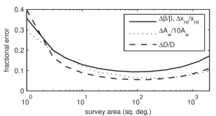
Figure 2: Ability of GBT to measure the BAO and redshift space distortions as a function of survey area at fixed observing time. Presented survey is between $z=0.54$ and $z=1.09$ and observing time is 1440 hours. A factor of 10 has been removed from the $A_{w}$ curve.

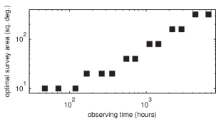
Figure 3: Roughly optimized survey area as a function of telescope time on GBT. Redshift range is between $z=0.54$ and $z=1.09$.

Prototyping for dedicated cylindrical telescopes is in its early stages. We present forecasts for a hypothetical not-too-far-off telescope, composed of two cylinders. The total array measures 40 m$\times$40 m with 300 dipole receivers with 200 MHz bandwidth, and a system temperature of 100 K. Such telescopes have no moving parts and point solely by the rotation of the earth. As such, the area of the survey is set by latitude, receiver spacing, and obstruction by foregrounds; we assume 15 000 square degrees. The survey area scales with the number of receivers leaving the noise per pixel unchanged. Thus the squared errors on measured quantities scale inversely with the number of receivers. Note that this is a slightly different scaling than the area optimized case of GBT, where it is the time axis that is scaled by the number of receivers. However, in the area optimized case variances also scale inversely with time as area optimization effectively fixes the noise per pixel. As such our results for GBT follow both scalings.

The forecasts for cylindrical telescopes are also applicable to pathfinder aperture arrays Faulkner et al. (2010). Where-as cylinders use optics to form a beam in one dimension and interferometry in the other, aperture arrays directly sample the incoming radio waves without optics. Interferometry is used in both dimensions, forming a two dimensional array of beams, instead of a two pixel wide strip for a two cylinder telescope. In principle it would be possible for an aperture array to monitor essentially the whole sky simultaneously, and thus form thousands of beams. In practise digitizing every antenna is costly and many antennas must be added in analogue in such a way that some beams are preserved but many are cancelled. We consider a compact aperture array that has the same area and resolution as the cylinder considered here. This is almost identical in scale as the proposed A3IV van Ardenne (2009). We assume preliminary A3IV specifications, with 700 effective receivers, 300 MHz bandwidth, and 50 K system temperature de Bruyn (2010). The aperture array could thus perform the same survey as the cylinder but a factor of $(300\,\mathrm{MHz}/200\,\mathrm{MHz})(700/300)(100\,\mathrm{K}/50\,\mathrm{K})^{2}=14$ faster. Note however, that for aperture arrays there is added freedom in which beams are preserved when antennas are added. It would be thus possible to optimize the area of the survey as in the GBT case.

Figures 4 and 5 show the obtainable fractional errors on RSD parameter $\beta$ and BAO parameters $A_{w}$, the amplitude of wiggles, and $D$ the overall dilation factor. $D$ is defined as a simultaneous dilation in both the longitudinal and transverse directions, i.e. both $H$ and $d_{A}$ are proportional to $D$. There is another “skew” parameter which trades one for the other, such that the Hubble parameter and the angular diameter distance can be independently determined, however, this parameter is generally not as precisely measured Padmanabhan and White (2008). $D$ is the mode that contains most of the information available in the BAO and we marginalize over the skew parameter. The marginalized error on $D$ is independent of the exact definition of the skew. Fractional errors on $H$ and $d_{A}$ are of order twice the fractional error on $D$.

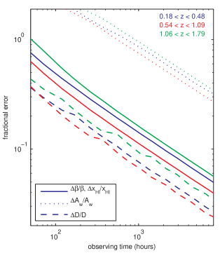
Figure 4: (Color online) Forecasts for fractional error on redshift space distortion and baryon acoustic oscillation parameters for intensity mapping surveys on the Green Bank Telescope (GBT). Frequency bins are approximately 200 MHz wide and correspond to available GBT receivers. Uncertainties on $D$ should not be trusted unless the uncertainty on $A_{w}$ is less than 50% (see text).

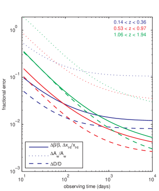
Figure 5: (Color online) Forecasts for fractional error on redshift space distortion and baryon acoustic oscillation parameters for intensity mapping surveys on a prototype cylindrical telescope. Frequency bins are 200 MHz wide corresponding to the capacity of the correlators which will likely be available. These result also apply to the aperture telescope but with the observing time reduced by a factor of 14. Uncertainties on $D$ should not be trusted unless the uncertainty on $A_{w}$ is less than 50% (see text). Observing time does not account for lost time due to foreground obstruction.

Referring to Figure 1 above, it can be seen intuitively that the parameters $D$ and $A_{w}$ are weakly correlated. Furthermore, since the signal is linear in the parameter $A_{w}$, our linear Fisher analysis applies even for large errors. This however cannot be said about $D$. Indeed any uncertainty on $D$, that brings the smallest scale peak we resolve more than $\sim\pi/2$ out of phase, cannot be trusted. It can be seen from Figure 1 that this corresponds to a fractional error of order 10%, which of course depends on resolution. For this reason, we require that the uncertainty on $A_{w}$ must be at most 50% (a 95% confidence detection of the BAO) before we have any faith in the uncertainty in $D$. We note that Fisher analysis is not the optimal tool for determining when an effect can first be measured; however, it applies for any cosmologically useful measurements of the BAO.

V Discussion

Typically measurements of the neutral hydrogen density at high redshift are made using damped Lyman-$\alpha$ (DLA) absorption lines; current measurement uncertainties being at the 25% statistical precision level in the $0.5<z<2$ redshift range Prochaska et al. (2005); Rao et al. (2006). However, it has been argued that these measurements are biased high Prochaska and Wolfe (2008) rendering the quantity effectively uncertain by a factor of 3. Hydrogen is the main baryonic component in the universe and it becomes neutral after falling into galaxies and becoming self shielded from ionizing radiation. As such, the abundance of neutral hydrogen is linked to the availability of fuel for star formation Wolfe et al. (1986); Pei and Fall (1995). Understanding how the neutral hydrogen evolves over cosmic time is key to understanding the star formation history and feedback processes in galaxy formation studies Wolfe et al. (2005); Shen et al. (2009). Additionally, the linear bias, and any scale dependence it might have, gives valuable information about how the gas is distributed. Finally, these quantities are crucial for estimating the sensitivity of future 21 cm redshift surveys since the signal is proportional to the product of the bias and the mean neutral density Chang et al. (2008).

We have shown that even with existing telescopes, it is possible to use 21 cm intensity mapping to make useful measurements of large scale structure at high redshift. As seen in Figure 4, a 4 $\sigma$ detection of redshift space distortions could be made at $z\approx 0.8$ with only 200 hours of telescope time at GBT. This would provide a 25% measurement of the neutral hydrogen fraction in the Universe using methods independent of DLA absorption lines. A longer survey using 1000 hours of telescope time could make $\sim$$12\%$ measurements.

Surveys extending to this level of precision become cosmologically useful. With 4000 observing hours on GBT (1000 hours with a four pixel receiver), the BAO overall distance scale could be measured to 3.5% precision at the same redshift. This is approaching the precision of the WiggleZ survey, which will make a $\sim$$2\%$ measurement of this scale over a similar redshift range Blake et al. (2009); Drinkwater et al. (2009). Because WiggleZ will make a similar measurement, such a survey would not have a dramatic effect on cosmological parameter estimations. However, it would provide an excellent verification of these measurements, using completely different methods, in different regions of the sky, and at low cost.

Prototypes for cylindrical telescopes could perform similar science to existing telescopes except—with dedicated resources—longer integration times would be feasible. This in part makes up for the limited resolution as for 40 m telescopes there is a substantial loss of information, and only the first wiggles are resolved. The measurements described here would constitute a proving ground for this technique. The success of these prototypes would be a clear indicator of the power and future success of full scale cylindrical telescopes.

The most powerful telescope considered is the aperture array, which would be capable of making sub present level BAO measurements with only a few weeks of dedicated observing. The design for demonstrator telescope A3IV has yet to be finalized but the proposed telescope is of nearly the same scale as the aperture array considered here. Depending on its eventual configuration, the A3IV could be a powerful probe of the Universe.

We have shown that 21 cm intensity mapping surveys could be employed in the short term to make useful measurements with large scale structure. With relatively small initial resource allocations, requisite techniques such as foreground subtraction can be tried and tested while performing valuable science. Such short term applications of this promising method will lay the trail for future dark energy surveys.