Krein Spaces in de Sitter Quantum Theories

Krein Spaces in de Sitter Quantum Theories

Jean-Pierre GAZEAU ^†, Petr SIEGL ^†‡ and Ahmed YOUSSEF ^†

J.-P. Gazeau, P. Siegl and A. Youssef

^† Astroparticules et Cosmologie (APC, UMR 7164), Université Paris-Diderot,
^† Boite 7020, 75205 Paris Cedex 13, France gazeau@apc.univ-paris7.fr, psiegl@apc.univ-paris7.fr, youssef@apc.univ-paris7.fr

^‡ Nuclear Physics Institute of Academy of Sciences of the Czech Republic,
^‡ 250 68 Řež, Czech Republic

Received October 19, 2009, in final form January 15, 2010; Published online January 27, 2010

Experimental evidences and theoretical motivations lead to consider the curved space-time relativity based on the de Sitter group $SO_{0}(1,4)$ or $Sp(2,2)$ as an appealing substitute to the flat space-time Poincaré relativity. Quantum elementary systems are then associated to unitary irreducible representations of that simple Lie group. At the lowest limit of the discrete series lies a remarkable family of scalar representations involving Krein structures and related undecomposable representation cohomology which deserves to be thoroughly studied in view of quantization of the corresponding carrier fields. The purpose of this note is to present the mathematical material needed to examine the problem and to indicate possible extensions of an exemplary case, namely the so-called de Sitterian massless minimally coupled field, i.e. a scalar field in de Sitter space-time which does not couple to the Ricci curvature.

de Sitter group; undecomposable representations; Krein spaces; Gupta–Bleuler triplet, cohomology of representations

81T20; 81R05; 81R20; 22E70; 20C35

1 Introduction

De Sitter and anti de Sitter space-times are, with Minkowski space-time, the only maximally symmetric space-time solutions in general relativity. Their respective invariance (in the relativity or kinematical sense) groups are the ten-parameter de Sitter $SO_{0}(1,4)$ and anti de Sitter $SO_{0}(2,3)$ groups. Both may be viewed as deformations of the proper orthochronous Poincaré group $\mathcal{P}^{1,3}\rtimes\,SO_{0}(1,3)$, the kinematical group of Minkowski space-time.

The de Sitter (resp. anti de Sitter) space-times are solutions to the vacuum Einstein’s equations with positive (resp. negative) cosmological constant $\Lambda$. This constant is linked to the (constant) Ricci curvature $4\Lambda$ of these space-times. The corresponding fundamental length is given by

$$R=\sqrt{\frac{3}{|\Lambda|}}=cH^{-1},$$ (1.1)

where $H$ is the Hubble constant.

Serious reasons back up any interest in studying Physics in such constant curvature spacetimes with maximal symmetry. The first one is the simplicity of their geometry, which makes us consider them as an excellent laboratory model in view of studying Physics in more elaborate universes, more precisely with the purpose to set up a quantum field theory as much rigorous as possible [19, 12, 32]. In this paper we are only interested in the de Sitter space-time. Indeed, since the beginning of the eighties, the de Sitter space, specially the spatially flat version of it, has been playing a much popular role in inflationary cosmological scenarii where it is assumed that the cosmic dynamics was dominated by a term acting like a cosmological constant. More recently, observations on far high redshift supernovae, on galaxy clusters, and on cosmic microwave background radiation suggested an accelerating universe. Again, this can be explained with such a term. For updated reviews and references on the subject, we recommend [22, 8] and [29]. On a fundamental level, matter and energy are of quantum nature. But the usual quantum field theory is designed in Minkowski spacetime. Many theoretical and observational arguments plead in favour of setting up a rigorous quantum field theory in de Sitter, and of comparing with our familiar minkowskian quantum field theory. As a matter of fact, the symmetry properties of the de Sitter solutions may allow the construction of such a theory (see [14, 6] for a review on the subject). Furthermore, the study of de Sitter space-time offers a specific interest because of the regularization opportunity afforded by the curvature parameter as a “natural” cutoff for infrared or other divergences.

On the other hand, some of our most familiar concepts like time, energy, momentum, etc, disappear. They really require a new conceptual approach in de Sitterian relativity. However, it should be stressed that the current estimate on the cosmological constant does not allow any palpable experimental effect on the level of high energy physics experiments, unless (see [15]) we deal with theories involving assumptions of infinitesimal masses like photon or graviton masses.

As was stressed by Newton and Wigner [27], the concept of an elementary system $($…$)$ is a description of a set of states which forms, in mathematical language, an irreducible representation space for the inhomogeneous Lorentz $({\simeq}$ Poincaré$)$ group. We naturally extend this point of view by considering elementary systems in the de Sitter arena as associated to elements of the unitary dual of $SO_{0}(1,4)$ or $Sp(2,2)$. The latter was determined a long time ago [31, 26, 11, 30] and is compounded of principal, complementary, and discrete series. Note that the de Sitter group has no unitary irreducible representation (UIR) analogous to the so-called “massless infinite spin” UIR of the Poincaré group. As the curvature parameter (or cosmological constant) goes to zero, some of the de Sitter UIR’s have a minskowskian limit that is physically meaningful, whereas the others have not. However, it is perfectly legitimate to study all of them within a consistent de Sitter framework, on both mathematical (group representation) and physical (field quantization) sides. It should be noticed that some mathematical questions on this unitary dual remain open, like the decomposition of the tensor product of two elements of the discrete series, or should at least be more clarified, like the explicit realization of representations lying at the lowest limit of the discrete series. Also, the quantization of fields for the latter representations is not known, at the exception of one of them, which is associated with the so-called “massless minimally coupled field” (mmc) in de Sitter [16, 17] and references therein.

The present paper is mainly concerned with this particular family of discrete series of representations. Their carrier spaces present or may display remarkable features: invariant subspace of null-norm states, undecomposable representation features, Gupta–Bleuler triplet, Krein space structure, and underlying cohomology [28]. In Section 2 is given the minimal background to make the reader familiar with de Sitter symmetries and the unitary dual of $Sp(2,2)$. In Section 3 we give a short account of the minkowskian content of elements of the unitary dual through group representation contraction procedures. Section 4 is devoted to the scalar representations of the de Sitter group and the associated wave equation. Then, in Section 5 we construct and control the normalizability of a class of scalar solutions or “hyperspherical modes” through de Sitter wave plane solutions [4, 6, 5] viewed as generating functions. The infinitesimal and global actions of the de Sitter group in its scalar unitary representations is described in Section 7. We then give a detailed account of the mmc case in Section 8. Finally a list of directions are given in Section 9 in view of future work(s). An appendix is devoted to the root system $B_{2}$ which corresponds to the de Sitter Lie algebra $so(1,4)$.

2 de Sitter space-time: geometric and quantum symmetries

We first recall that the de Sitter space-time is conveniently described as the one-sheeted hyperboloid embedded in a 4+1-dimensional Minkowski space, here denoted $\mathbb{M}_{5}$:

$$M_{H}\equiv\big{\{}x\in\mathbb{M}_{5};\ x^{2}:=x\cdot x=\eta_{\alpha\beta}x^{\alpha}x^{\beta}=-H^{2}\big{\}},$$

$$\alpha,\beta=0,1,2,3,4,\qquad\left(\eta_{\alpha\beta}\right)=\mathrm{diag}(1,-1,-1,-1,-1),$$

with the so-called ambient coordinates notations

$$x:=\big{(}x^{0},\vec{x},x^{4}\big{)}.$$

The following intrinsic coordinates

$$x=\big{(}x^{0}=H^{-1}\tan\rho,(H\cos\rho)^{-1}u\big{)},\qquad\rho\in\big{]}{-}\tfrac{\pi}{2},\tfrac{\pi}{2}\big{[},\qquad u\in S^{3}\,$$ (2.1)

are global. They are usually called “conformal”.

There exist ten Killing vectors in de Sitterian kinematics. They generate the Lie algebra $so(1,4)$, which gives by exponentiation the de Sitter group $SO_{0}(1,4)$ or its universal covering $Sp(2,2)$. In unitary irreducible representations of the latter, they are represented as (essentially) self-adjoint operators in Hilbert space of (spinor-) tensor valued functions on $M_{H}$, square integrable with respect to some invariant inner (Klein–Gordon type) product:

$$K_{\alpha\beta}\rightarrow L_{\alpha\beta}=M_{\alpha\beta}+S_{\alpha\beta},$$ (2.2)

where

$$M_{\alpha\beta}=-i(x_{\alpha}\partial_{\beta}-x_{\beta}\partial_{\alpha})$$

is the “orbital part”, and $S_{\alpha\beta}$ (spinorial part) acts on indices of functions in a certain permutational way.

There are two Casimir operators, the eigenvalues of which determine the UIR’s:

$$\mathcal{C}_{2}=-\tfrac{1}{2}L_{\alpha\beta}L^{\alpha\beta}\qquad(\mbox{quadratic}),$$

$$\mathcal{C}_{4}=-W_{\alpha}W^{\alpha},\qquad W_{\alpha}=-\tfrac{1}{8}\epsilon_{\alpha\beta\gamma\delta\eta}L^{\beta\gamma}L^{\delta\eta}\qquad(\mbox{quartic}).$$

In a given UIR, and with the Dixmier notations [11], these two Casimir operators are fixed as

$$\mathcal{C}_{2}=(-p(p+1)-(q+1)(q-2))\mathbb{I},$$ (2.3)

$$\mathcal{C}_{4}=(-p(p+1)q(q-1))\mathbb{I}$$ (2.4)

with specific allowed range of values assumed by parameters $p$ and $q$ for the three series of UIR, namely discrete, complementary, and principal.

“Discrete series” $\boldsymbol{\Pi^{\pm}_{p,q}}$

Parameter $q$ has a spin meaning. We have to distinguish between

• the scalar case $\Pi_{p,0}$, $p=1,2,\dots$. These representations lie at the “lowest limit” of the discrete series and are not square integrable,

• the spinorial case $\Pi^{\pm}_{p,q}$, $q>0$, $p=\frac{1}{2},1,\frac{3}{2},2,\dots$, $q=p,p-1,\dots,1$ or $\frac{1}{2}$. For $q=\frac{1}{2}$ the representations $\Pi^{\pm}_{p,\frac{1}{2}}$ are not square-integrable.

“Principal series” $\boldsymbol{U_{s,\nu}}$

$$q=\tfrac{1}{2}\pm i\nu.$$

$p=s$ has a spin meaning and the two Casimir are fixed as

$$\mathcal{C}_{2}=\big{(}\tfrac{9}{4}+\nu^{2}-s(s+1)\big{)}\mathbb{I},\qquad\mathcal{C}_{4}=\big{(}\tfrac{1}{4}+\nu^{2}\big{)}s(s+1)\mathbb{I}.$$

We have to distinguish between

• $\nu\in\mathbb{R}$, $s=1,2,\dots$, for the integer spin principal series,

• $\nu\neq 0$, $s=\frac{1}{2},\frac{3}{2},\frac{5}{2},\dots$, for the half-integer spin principal series.

In both cases, $U_{s,\nu}$ and $U_{s,-\nu}$ are equivalent. In the case $\nu=0$, i.e. $q=\frac{1}{2}$, $s=\frac{1}{2},\frac{3}{2},\frac{5}{2},\dots$, the representations are not irreducible. They are direct sums of two UIR’s belonging to the discrete series:

$$U_{s,0}=\Pi^{+}_{s,\frac{1}{2}}\bigoplus\Pi^{-}_{s,\frac{1}{2}}.$$

“Complementary series” $\boldsymbol{V_{s,\nu}}$

$$q=\tfrac{1}{2}\pm\nu.$$

$p=s$ has a spin meaning and the two Casimir are fixed as

$$\mathcal{C}_{2}=\big{(}\tfrac{9}{4}-\nu^{2}-s(s+1)\big{)}\mathbb{I},\qquad\mathcal{C}_{4}=\big{(}\tfrac{1}{4}-\nu^{2}\big{)}s(s+1)\mathbb{I}.$$

We have to distinguish between

• the scalar case $V_{0,\nu}$, $\nu\in\mathbb{R}$, $0<|\nu|<\frac{3}{2}$,

• the spinorial case $V_{s,\nu}$, $0<|\nu|<\frac{1}{2}$, $s=1,2,3,\dots$.

In both cases, $V_{s,\nu}$ and $V_{s,-\nu}$ are equivalent.

3 Contraction limits or de Sitterian physics
from the point of view of a Minkowskian observer

At this point, it is crucial to understand the physical content of these representations in terms of their null curvature limit, i.e., from the point of view of local (“tangent”) minkowskian observer, for which the basic physical conservation laws are derived from Einstein–Poincaré relativity principles. We will distinguish between those representations of the de Sitter group which contract to Poincaré massive UIR’s, those which have a massless content, and those which do not have any flat limit at all. Firstly let us explain what we mean by null curvature limit on a geometrical and algebraic level.

On a geometrical level:

$\lim\limits_{H\to 0}M_{R}=\mathbb{M}_{4}$, the Minkowski spacetime tangent to $M_{H}$ at, say, the de Sitter “origin” point $O\stackrel{{\scriptstyle\mathrm{def}}}{{=}}(0,\vec{0},H^{-1})$.

On an algebraic level:

• $\lim\limits_{R\to\infty}Sp(2,2)={\cal P}^{\uparrow}_{+}(1,3)=\mathbb{M}_{4}\rtimes SL(2,\mathbb{C})$, the Poincaré group.

• The ten de Sitter Killing vectors contract to their Poincaré counterparts $K_{\mu\nu}$, $\Pi_{\mu}$, $\mu=0,1,2,3$, after rescaling the four $K_{4\mu}\longrightarrow\Pi_{\mu}=HK_{4\mu}$.

3.1 de Sitter UIR contraction: the massive case

For what we consider as the “massive” case, principal series representations only are involved (from which the name “de Sitter massive representations”). Introducing the Poincaré mass $m=\nu/R$ [24, 13, 15], we have:

$$U_{s,\nu}\underset{R\to\infty,\nu\to\infty}{\longrightarrow}{c_{>}\cal P}^{>}(m,s)\oplus c_{<}{\cal P}^{<}(m,s),$$

where one of the “coefficients” among $c_{<}$, $c_{>}$ can be fixed to 1 whilst the other one vanishes and where ${\cal P}^{\stackrel{{\scriptstyle>}}{{<}}}(m,s)$ denotes the positive (resp. negative) energy Wigner UIR’s of the Poincaré group with mass $m$ and spin $s$.

3.2 de Sitter UIR contraction: the massless case

Here we must distinguish between

• the scalar massless case, which involves the unique complementary series UIR $V_{0,1/2}$ to be contractively Poincaré significant,

• and the helicity $s\neq 0$ case where are involved all representations $\Pi^{\pm}_{s,s}$, $s>0$ lying at the lower limit of the discrete series.

The arrows $\hookrightarrow$ below designate unique extension. Symbols ${\cal P}^{\overset{>}{<}}(0,s)$ denote the Poincaré massless representations with helicity $s$ and with positive (resp. negative) energy. Conformal invariance involves the discrete series representations (and their lower limits) of the (universal covering of the) conformal group or its double covering $SO_{0}(2,4)$ or its fourth covering $SU(2,2)$. These UIR’s are denoted by ${\cal C}^{\stackrel{{\scriptstyle>}}{{<}}}(E_{0},j_{1},j_{2})$, where $(j_{1},j_{2})\in\mathbb{N}/2\times\mathbb{N}/2$ labels the UIR’s of $SU(2)\times SU(2)$ and $E_{0}$ stems for the positive (resp. negative) conformal energy.

• Scalar massless case:

  $$\left.\begin{array}[]{ccccccc}&&{\cal C}^{>}(1,0,0)&&{\cal C}^{>}(1,0,0)&\hookleftarrow&{\cal P}^{>}(0,0)\\ V_{0,1/2}&\hookrightarrow&\oplus&\stackrel{{\scriptstyle R\to\infty}}{{\longrightarrow}}&\oplus&&\oplus\\ &&{\cal C}^{<}(-1,0,0)&&{\cal C}^{<}(-1,0,0)&\hookleftarrow&{\cal P}^{<}(0,0).\\ \end{array}\right.$$

• Spinorial massless case:

  $$\left.\begin{array}[]{ccccccc}&&{\cal C}^{>}(s+1,s,0)&&{\cal C}^{>}(s+1,s,0)&\hookleftarrow&{\cal P}^{>}(0,s)\\ \Pi^{+}_{s,s}&\hookrightarrow&\oplus&\stackrel{{\scriptstyle R\to\infty}}{{\longrightarrow}}&\oplus&&\oplus\\ &&{\cal C}^{<}(-s-1,s,0)&&{\cal C}^{<}(-s-1,s,0)&\hookleftarrow&{\cal P}^{<}(0,s),\\ \end{array}\right.$$

  $$\left.\begin{array}[]{ccccccc}&&{\cal C}(s+1,0,s)&&{\cal C}^{>}(s+1,0,s)&\hookleftarrow&{\cal P}^{>}(0,-s)\\ \Pi^{-}_{s,s}&\hookrightarrow&\oplus&\stackrel{{\scriptstyle R\to\infty}}{{\longrightarrow}}&\oplus&&\oplus\\ &&{\cal C}^{<}(-s-1,0,s)&&{\cal C}^{<}(-s-1,0,s)&\hookleftarrow&{\cal P}^{<}(0,-s).\\ \end{array}\right.$$

4 Scalar representations

In the present study, we are concerned with scalar fields only, for which the value of the quartic Casimir vanishes. Two cases are possible: $p=0$ for the principal and complementary series, and $q=0$ for the discrete series. In both cases, the fields carrying the representations are solutions of the scalar quadratic “wave equations” issued from equation (2.4):

$$\mathcal{C}_{2}\psi(x)\equiv Q_{0}\psi(x)=-(p-1)(p+2)\psi(x),$$ (4.1)

for the scalar discrete series, and

$$\mathcal{C}_{2}\psi(x)\equiv Q_{0}\psi(x)=-(q+1)(q-2)\psi(x),$$ (4.2)

for the scalar principal and complementary series. Let us define the symmetric, “transverse projector”

$$\theta_{\alpha\beta}=\eta_{\alpha\beta}+H^{2}x_{\alpha}x_{\beta}$$

which satisfies $\theta_{\alpha\beta}x^{\alpha}=\theta_{\alpha\beta}x^{\beta}=0$. It is the transverse form of the de Sitter metric in ambient space notations and it is used in the construction of transverse entities like the transverse derivative

$$\bar{\partial}_{\alpha}=\theta_{\alpha\beta}\partial^{\beta}=\partial_{\alpha}+H^{2}x_{\alpha}x.\partial.$$

With these notations, the scalar Casimir operator reads as $Q_{0}=-H^{-2}\bar{\partial}^{2}$ and equations (4.1) and (4.2) become

$$(Q_{0}+\sigma(\sigma+3))\psi(x)=-H^{-2}\bar{\partial}^{2}\psi(x)+\sigma(\sigma+3)\psi(x)=0,$$ (4.3)

where we have introduced the unifying complex parameter $\sigma$. As is shown in Fig. 1, $\sigma=p-1$ or $=-p-2$ for the scalar discrete series, $\sigma=-q-1=-3/2-i\nu$ for the scalar principal series, and $\sigma=-q-1=-3/2-\nu$ for the scalar complementary series. Actually, we will examine this equation for any complex value of the parameter $\sigma$, proceeding with appropriate restrictions when is necessary. Just note that the scalar discrete series starts with the so-called massless minimally coupled” (mmc) case, exactly there where the complementary series ends on its left.

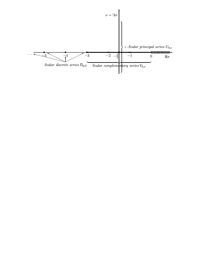
Figure 1: Indexing the set of scalar UIR with complex parameter $\sigma$. It should be remembered that representations $U_{0,\nu}$ and $U_{0,-\nu}$ with $\sigma=-3/2-i\nu$ in the principal series, and $V_{0,\nu}$ and $V_{0,-\nu}$ with $\sigma=-3/2-\nu$ in the complementary series (i.e. under symmetry $\sigma\mapsto-3-\sigma$) are equivalent. The “massless minimally coupled” representation corresponds to $\sigma=-3$. The “conformally invariant massless” scalar representation corresponds to $\sigma=-2$, or equivalently to $\sigma=-1$. The case $\sigma=0$ can be viewed as corresponding to the trivial representation.

5 de Sitter wave planes as generating functions

There exists a continuous family of simple solutions (“de Sitter plane waves”) to equation (4.3). These solutions, as indexed by vectors $\xi$ lying in the null-cone in $\mathbb{M}_{5}$:

$$\xi=(\xi^{0},\boldsymbol{\xi})\in\mathcal{C}\stackrel{{\scriptstyle\mathrm{def}}}{{=}}\left\{\xi\in\mathbb{M}_{5}:\xi^{2}=0\right\},$$

read

$$\psi(x)=(Hx\cdot\xi)^{\sigma}.$$

Putting $\boldsymbol{\xi}=\|\boldsymbol{\xi}\|v\in\mathbb{R}^{4}$, $v\in S^{3}$, and $|\xi^{0}|=\|\boldsymbol{\xi}\|$, we rewrite the dot product $Hx\cdot\xi$ as follows

$$Hx\cdot\xi=(\tan{\rho})\,\xi^{0}-\frac{1}{\cos{\rho}}u\cdot\boldsymbol{\xi}=\frac{\xi^{0}e^{i\rho}}{2i\,\cos{\rho}}\big{(}1+z^{2}-2zt\big{)}$$

$$\phantom{Hx\cdot\xi=}{}\mbox{with}\ z=ie^{-i\rho}\mathrm{sgn}\,{\xi^{0}},\qquad t=u\cdot v=:\cos{\varpi}.$$

By using the generating function for Gegenbauer polynomials,

$$\big{(}1+z^{2}-2zt\big{)}^{-\lambda}=\sum_{n=0}^{\infty}z^{n}\,C_{n}^{\lambda}(t),\qquad|z|<1,$$ (5.1)

we get the expansion

$$(Hx\cdot\xi)^{\sigma}=\left(\frac{\xi^{0}e^{i\rho}}{2i\,\cos{\rho}}\right)^{\sigma}\big{(}1+z^{2}-2zt\big{)}^{\sigma}=\left(\frac{\xi^{0}e^{i\rho}}{2i\,\cos{\rho}}\right)^{\sigma}\sum_{n=0}^{\infty}z^{n}C_{n}^{-\sigma}(t),\qquad\Re{\sigma}<\frac{1}{2}.$$ (5.2)

This expansion is actually not valid in the sense of functions since $|z|=1$. However, giving a negative imaginary part to the angle $\rho$ ensures the convergence. This amounts to extend ambient coordinates to the forward tube [6]:

$$\mathcal{T}^{+}=\big{\{}\mathbb{M}_{5}-i\overline{V}_{5}^{+}\cap M_{H}^{\scriptscriptstyle\mathbb{C}}\big{\}},\qquad\overline{V}_{5}^{+}=\big{\{}x\in\mathbb{M}_{5}:x^{2}\geq 0,x^{0}>0\big{\}}.$$

We now make use of two expansion formulas involving Gegenbauer polynomials [18] and $S^{3}$ normalized hyperspherical harmonics:

$$C_{n}^{\lambda}(t)=\frac{1}{\Gamma(\lambda)\Gamma(\lambda-1)}\sum_{k=0}^{\lfloor\frac{n}{2}\rfloor}c_{k}C_{n-2k}^{1}(t),$$

$$c_{k}=\frac{(n-2k+1)\Gamma(k+\lambda-1)\Gamma(\lambda+n-k)}{k!\Gamma(n-k+2)},$$ (5.3)

$$C_{L}^{1}(v\cdot v^{\prime})=\frac{2\pi^{2}}{L+1}\sum_{lm}\mathrm{Y}_{Llm}(v)\mathrm{Y}^{\ast}_{Llm}(v^{\prime}),\qquad v,v^{\prime}\in S^{3}.$$ (5.4)

We recall here the expression of the hyperspherical harmonics:

$$\mathrm{Y}_{Llm}(u)=\left(\frac{(L+1)(2l+1)(L-l)!}{2\pi^{2}(L+l+1)!}\right)^{\frac{1}{2}}2^{l}l!\left(\sin\alpha\right)^{l}C_{L-l}^{l+1}\left(\cos\alpha\right)Y_{lm}(\theta,\phi),$$ (5.5)

for $(L,l,m)\in\mathbb{N}\times\mathbb{N}\times\mathbb{Z}$ with $0\leq l\leq L$ and $-l\leq m\leq l$. In this equation the $Y_{lm}$’s are ordinary spherical harmonics:

$$Y_{lm}(\theta,\phi)=(-1)^{m}\left(\frac{(l-m)!}{(l+m)!}\right)^{\frac{1}{2}}P_{l}^{m}(\cos\theta)e^{im\phi},$$

where the $P_{l}^{m}$’s are the associated Legendre functions. With this choice of constant factors, the $\mathrm{Y}_{Llm}$’s obey the orthogonality (and normalization) conditions:

$$\int_{S^{3}}\mathrm{Y}_{Llm}^{*}(u)\mathrm{Y}_{L^{\prime}l^{\prime}m^{\prime}}(u)\,du=\delta_{LL^{\prime}}\delta_{ll^{\prime}}\delta_{mm^{\prime}}.$$

Combining (5.1), (5.3) and (5.4) we get the expansion formula:

$$\big{(}1+z^{2}-2zv\cdot v^{\prime}\big{)}^{-\lambda}=2\pi^{2}\sum_{Llm}z^{L}p^{\lambda}_{L}\big{(}z^{2}\big{)}\mathrm{Y}_{Llm}(v)\mathrm{Y}^{\ast}_{Llm}(v^{\prime}),$$ (5.6)

where

$$p^{\lambda}_{L}\big{(}z^{2}\big{)}=\frac{1}{(L+1)!}\frac{\Gamma(\lambda+L)}{\Gamma(\lambda)}{}_{2}F_{1}\big{(}L+\lambda,\lambda-1;L+2;z^{2}\big{)}$$

and the integral representation,

$$z^{L}p^{\lambda}_{L}\big{(}z^{2}\big{)}\mathrm{Y}_{Llm}(v)=\frac{1}{2\pi^{2}}\int_{S^{3}}\big{(}1+z^{2}-2zv\cdot v^{\prime}\big{)}^{-\lambda}\mathrm{Y}_{Llm}(v^{\prime})d\mu(v^{\prime}).$$

Let us apply the above material to the de Sitter plane waves $(Hx\cdot\xi)^{\sigma}$. In view of equations (5.2) and (5.6) with $\lambda=-\sigma$, we introduce the set of functions on the de Sitter hyperboloid:

$$\Phi_{Llm}^{\sigma}(x)=\frac{i^{L-\sigma}e^{-i(L-\sigma)\rho}}{(2\cos{\rho})^{\sigma}}p^{-\sigma}_{L}\big{(}{-}e^{-2i\rho}\big{)}\mathrm{Y}_{Llm}(u)$$

$$\phantom{\Phi_{Llm}^{\sigma}(x)}{}=\frac{i^{L-\sigma}e^{-i(L-\sigma)\rho}}{(2\cos{\rho})^{\sigma}}\frac{\Gamma(L-\sigma)}{(L+1)!\Gamma(-\sigma)}\,{}_{2}F_{1}\big{(}L-\sigma,-\sigma-1;L+2;-e^{-2i\rho}\big{)}\mathrm{Y}_{Llm}(u).\!\!$$ (5.7)

By using the well-known relation between hypergeometric functions [23],

$${}_{2}F_{1}(a,b;c;z)=(1-z)^{c-a-b}\,{}_{2}F_{1}(c-a,c-b;c;z),$$

we get the alternative form of (5.7)

$$\Phi_{Llm}^{\sigma}(x)=i^{L-\sigma}\,e^{-i(L+\sigma+3)\rho}(2\cos{\rho})^{\sigma+3}\frac{\Gamma(L-\sigma)}{(L+1)!\Gamma(-\sigma)}$$

$$\phantom{\Phi_{Llm}^{\sigma}(x)=}{}\times{}_{2}F_{1}\big{(}\sigma+2,L+\sigma+3;L+2;-e^{-2i\rho}\big{)}\mathrm{Y}_{Llm}(u).$$ (5.8)

We then have the expansion of the de Sitter plane waves:

$$(Hx\cdot\xi)^{\sigma}=2\pi^{2}\sum_{Llm}\Phi_{Llm}^{\sigma}(x)\big{(}\xi^{0}\big{)}^{\sigma}\big{(}\mathrm{sgn}\,{\xi^{0}}\big{)}^{L}\mathrm{Y}^{\ast}_{Llm}(v).$$

From the linear independence of the hyperspherical harmonics, it is clear that the functions $\Phi_{Llm}^{\sigma}(x)$ are solutions to the scalar wave equation (4.3) once one has proceeded with the appropriate separation of variables, a question that we examine in the next section. From the orthonormality of the set of hyperspherical harmonics we have the integral representation (“Fourier transform” on $S^{3}$),

$$\Phi_{Llm}^{\sigma}(x)=\frac{\big{(}\mathrm{sgn}\,{\xi^{0}}\big{)}^{L}}{2\pi^{2}(\xi^{0})^{\sigma}}\int_{S^{3}}d\mu(v)(Hx\cdot\xi)^{\sigma}\mathrm{Y}_{Llm}(v).$$

We notice that the functions $\Phi_{Llm}^{\sigma}(x)$ are well defined for all $\sigma$ such that $\Re\sigma<0$, so for all scalar de Sitter UIR, and are infinitely differentiable in the conformal coordinates $(\rho,u)$ in their respective ranges. At the infinite de Sitter “past” and “future”, i.e. at the limit $\rho=\pm\pi/2$, their behavior is ruled by the factor $(\cos{\rho})^{\sigma+3}$:

$$\Phi_{Llm}^{\sigma}(x)\simeq_{\rho\to\pm\pi/2}i^{L-\sigma}e^{-i(L+\sigma+3)\rho}(2\,\cos{\rho})^{\sigma+3}\frac{\Gamma(-2\sigma-1)}{(L+1)!\Gamma(-\sigma)\Gamma(-\sigma-1)}\mathrm{Y}_{Llm}(u),$$

where we have used the formula [23]

$${}_{2}F_{1}(a,b;c;1)=\frac{\Gamma(c)\Gamma(c-a-b)}{\Gamma(c-a)\Gamma(c-b)}$$

valid for $\Re(c-a-b)>0$ and $c\neq-1,-2,\dots$. The singularity that appears for $\Re\sigma<-3$, which is the case for the scalar discrete series with $p\geq 2$, is due to the choice of conformal coordinates in expressing the dot product $\xi\cdot x$.

We now ask the question about the nature of the above functions as basis elements of some specific vector space of solutions to equation (4.3). For that we first introduce the so-called Klein–Gordon inner product in the space of solutions to (4.3), defined for solutions $\Phi_{1}$, $\Phi_{2}$ by

$$\langle\Phi_{1},\Phi_{2}\rangle=i\int_{\Sigma}\Phi_{1}^{*}(x)\big{(}\overrightarrow{\partial}_{\mu}-\overleftarrow{\partial}_{\mu}\big{)}\Phi_{2}(x)\,d\sigma^{\mu}\equiv i\int_{\Sigma}\Phi_{1}^{*}\stackrel{{\scriptstyle\leftrightarrow}}{{\partial}}_{\mu}\Phi_{2}\,d\sigma^{\mu},$$ (5.9)

where $\Sigma$ is a Cauchy surface, i.e. a space-like surface such that the Cauchy data on $\Sigma$ define uniquely a solution of (4.3), and $d\sigma^{\mu}$ is the area element vector on $\Sigma$. This product is de Sitter invariant and independent of the choice of $\Sigma$. In accordance with our choice of global coordinate system, the Klein–Gordon product (5.9) reads as

$$\langle\Phi_{1},\Phi_{2}\rangle=\frac{i}{H^{2}}\int_{\rho=0}\Phi_{1}^{*}(\rho,u)\stackrel{{\scriptstyle\leftrightarrow}}{{\partial}}_{\rho}\Phi_{2}(\rho,u)\,du,$$

where $du=\sin^{2}\alpha\sin\theta\,d\alpha\,d\theta\,d\phi$ is the invariant measure on $S^{3}$. Due to the orthogonality of the hyperspherical harmonics, the set of functions $\Phi_{Llm}^{\sigma}(x)$ is orthogonal:

$$\langle\Phi_{L_{1}l_{1}m_{1}}^{\sigma},\Phi_{L_{2}l_{2}m_{2}}^{\sigma}\rangle=\delta_{L_{1}L_{2}}\delta_{l_{1}l_{2}}\delta_{m_{1}m_{2}}\|\Phi_{L_{1}l_{1}m_{1}}^{\sigma}\|^{2},$$

in case of normalizable states. Let us calculate this norm:

$$\|\Phi_{Llm}^{\sigma}\|^{2}=\frac{\pi\,2^{2-2L}}{H^{2}}e^{-\pi\Im\sigma}\left|\frac{(\Gamma(L-\sigma)}{(\Gamma(-\sigma)}\right|^{2}$$

$$\phantom{\|\Phi_{Llm}^{\sigma}\|^{2}=}{}\times\Re\left[\Gamma^{\ast}\left(\frac{L-\sigma+1}{2}\right)\Gamma\left(\frac{L-\sigma}{2}\right)\Gamma^{\ast}\left(\frac{L+\sigma+4}{2}\right)\Gamma\left(\frac{L+\sigma+3}{2}\right)\right]^{-1}.$$ (5.10)

For real values of $\sigma$, in particular for the complementary series and, with restrictions for the discrete series (see below), the norm simplifies to:

$$\|\Phi_{Llm}^{\sigma}\|^{2}=\frac{2^{3}}{H^{2}}\frac{\Gamma(L-\sigma)}{(\Gamma(-\sigma))^{2}\Gamma(L+\sigma+3)}.$$ (5.11)

We see that for the scalar principal and complementary series all these functions are normalizable and are suitable candidates for scalar fields in de Sitter space-time carrying their respective UIR.

For the discrete series, $\sigma=-p-2$, $p=1,2,\dots,$ the hypergeometric functions reduce to polynomials of degree $p$, ${}_{2}F_{1}(-p,L-p+1;L+2;-e^{-2i\rho})$, and the norm vanishes for states with $L=0,1,\dots,p-1$. We will interpret this invariant $N$-dimensional null-norm subspace, $N=p(p+1)(2p+1)/6$, as a space of “gauge” states, carrying the irreducible (non-unitary!) de Sitter finite-dimensional representation $(n_{1}=0,n_{2}=p-1)$ (with the notations of Appendix A), which is “Weyl equivalent” to the UIR $\Pi_{p,0}$, i.e. shares with it the same eigenvalue of the Casimir operator $\mathcal{C}_{2}$.

For the regular case $L\geq p$, one can re-express the $\rho$-dependent part of the functions $\Phi_{Llm}^{\sigma}\equiv\Phi_{p;Llm}$ in terms of Gegenbauer polynomials:

$$\Phi_{p;Llm}(x)=-i^{L+p}2^{1-p}\frac{(L+p+1)!(L-p)!}{(L!)^{2}(L+1)(p+1)}$$

$$\phantom{\Phi_{p;Llm}(x)=}{}\times e^{-i(L+1)\rho}(\cos{\rho})^{1-p}C^{L-p+1}_{p}(\sin{\rho})\mathrm{Y}_{Llm}(u).$$

In the allowed ranges of parameters, the normalized functions [9] are defined as:

$$\Psi_{Llm}^{\sigma}(x)=\mathcal{N}_{L}^{\sigma}i^{L-\sigma}e^{-i(L+\sigma+3)\rho}(\cos\rho)^{\sigma+3}\,{}_{2}F_{1}(\sigma+1,L+\sigma+3;L+2;-e^{-2i\rho})\mathrm{Y}_{Llm}(u),$$

$$\mathcal{N}_{L}^{\sigma}=\frac{H}{\sqrt{\pi}}2^{L+\sigma+2}e^{\frac{\pi}{2}\Im\sigma}\frac{\Gamma(L-\sigma)}{|\Gamma(L-\sigma)|}\frac{|\Gamma(-\sigma)|}{\Gamma(-\sigma)}\frac{1}{(L+1)!}$$

$$\phantom{\mathcal{N}_{L}^{\sigma}=}{}\times\left[\Re\left(\Gamma^{\ast}\left(\frac{L-\sigma+1}{2}\right)\Gamma\left(\frac{L-\sigma}{2}\right)\Gamma^{\ast}\left(\frac{L+\sigma+4}{2}\right)\Gamma\left(\frac{L+\sigma+3}{2}\right)\right)\right]^{1/2}.$$ (5.12)

In the complementary and discrete series, $\sigma$ is real and, due to the duplication formula for the gamma function, the expression between brackets reduces to $\pi 2^{2-2L-3}\Gamma(L-\sigma)\Gamma(L+\sigma+3)$. Then the normalization factor simplifies to:

$$\mathcal{N}_{L}^{\sigma}=H2^{\sigma+1/2}\frac{\sqrt{\Gamma(L-\sigma)\Gamma(L+\sigma+3)}}{(L+1)!}.$$

Finally, in the scalar discrete series, with $\sigma=-p-2$, one gets for $L\geq p$ the orthonormal system:

$$\Psi_{Llm}^{\sigma}(x)\equiv\Psi_{p;Llm}(x)=-\mathcal{N}_{p;L}i^{L+p}e^{-i(L+1-p)\rho}(\cos\rho)^{1-p}$$

$$\phantom{\Psi_{Llm}^{\sigma}(x)\equiv\Psi_{p;Llm}(x)=}{}\times{}_{2}F_{1}\big{(}-p,L+1-p;L+2;-e^{-2i\rho}\big{)}\mathrm{Y}_{Llm}(u),$$

$$\mathcal{N}_{p;L}=2^{-p-1/2}\frac{\sqrt{\Gamma(L-p+1)\Gamma(L+p+2)}}{(L+1)!},\qquad L\geq p.$$

As noticed above, those functions become singular at the limits $\rho=\pm\pi/2$ at the exception of the lowest case (“minimally coupled massless field”) $p=1$. Going back to the de Sitter plane waves as generating functions, one gets the expansion in terms of orthonormal sets for the scalar principal or complementary series:

$$(Hx\cdot\xi)^{\sigma}=2\pi^{2}\sum_{Llm}\|\Phi^{\sigma}_{Llm}\|\Psi^{\sigma}_{Llm}(x)\big{(}\xi^{0}\big{)}^{\sigma}\big{(}\mathrm{sgn}\,\xi^{0}\big{)}^{L}Y^{\ast}_{Llm}(v),$$

where $\|\Phi^{\sigma}_{Llm}\|$ is given by (5.10) (principal) and by (5.11) (complementary). For the scalar discrete series, we have to split the sum into two parts:

$$(Hx\cdot\xi)^{-p-2}=2\pi^{2}\sum_{L=0}^{p-1}\sum_{lm}\Phi_{p;Llm}(x)\big{(}\xi^{0}\big{)}^{-p-2}\big{(}\mathrm{sgn}\,{\xi^{0}}\big{)}^{L}\mathrm{Y}^{\ast}_{Llm}(v)$$

$$\phantom{(Hx\cdot\xi)^{-p-2}=}{}+2\pi^{2}\sum_{L=p}^{\infty}\sum_{lm}\|\Phi_{p;Llm}\|\Psi_{p;Llm}(x)\big{(}\xi^{0}\big{)}^{-p-2}\big{(}\mathrm{sgn}\xi^{0}\big{)}^{L}Y^{\ast}_{Llm}(v).$$

These formulae make explicit the “spherical” modes in de Sitter space-time in terms of de Sitter plane waves.

6 Wave equation for scalar de Sitter representations

Let us check how we recover the functions $\Phi^{\sigma}_{Llm}$ or $\Psi^{\sigma}_{Llm}$ by directly solving the wave equation. The scalar Casimir operator $Q_{0}$ introduced in (4.1) and (4.2) is just proportional to the Laplace–Beltrami operator on de Sitter space: $Q_{0}=-H^{-2}\square$. In terms of the conformal coordinates (2.1) the latter is given by

$$\square=\frac{1}{\sqrt{g}}\partial_{\nu}\sqrt{g}g^{\nu\mu}\partial_{\mu}=H^{2}\cos^{4}\rho\frac{\partial}{\partial\rho}\left(\cos^{-2}\rho\frac{\partial}{\partial\rho}\right)-H^{2}\cos^{2}\rho\Delta_{3},$$

where

$$\Delta_{3}=\frac{\partial^{2}}{\partial\alpha^{2}}+2\cot\alpha\frac{\partial}{\partial\alpha}+\frac{1}{\sin^{2}\alpha}\frac{\partial^{2}}{\partial\theta^{2}}+\cot\theta\frac{1}{\sin^{2}\alpha}\frac{\partial}{\partial\theta}+\frac{1}{\sin^{2}\alpha\sin^{2}\theta}\frac{\partial^{2}}{\partial\phi^{2}}$$

is the Laplace operator on the hypersphere $S^{3}$. Equation (4.2) can be solved by separation of variable [9, 21]. We put

$$\psi(x)=\chi(\rho)D(u),$$

where $u\in S^{3}$, and obtain

$$[\Delta_{3}+C]D(u)=0,$$ (6.1)

$$\left(\cos^{4}\rho\frac{d}{d\rho}\cos^{-2}\rho\frac{d}{d\rho}+C\cos^{2}\rho-\sigma(\sigma+3)\right)\chi(\rho)=0.$$ (6.2)

We begin with the angular part problem (6.1). For $C=L(L+2)$, $L\in\mathbb{N}$ we find the hyperspherical harmonics $D=\mathrm{Y}_{Llm}$ which are defined in (5.5).

For the $\rho$ dependent part, and for $\sigma$ we obtain the solutions in terms of Legendre functions on the cut

$$\chi_{\sigma;L}(\rho)=A_{L}(\cos\rho)^{\frac{3}{2}}\left[P^{\lambda}_{L+\frac{1}{2}}(\sin\rho)-\frac{2i}{\pi}Q^{\lambda}_{L+\frac{1}{2}}(\sin\rho)\right].$$

Here $\lambda=\pm(\sigma+3/2)$ and $A_{L}$ is given by

$$A_{L}=H\frac{\sqrt{\pi}}{2}\left(\frac{\Gamma\big{(}L-\lambda+\frac{3}{2}\big{)}}{\Gamma\big{(}L+\lambda+\frac{3}{2}\big{)}}\right)^{\frac{1}{2}}.$$

We then obtain the set of solutions

$$\Psi_{Llm}^{\sigma}(x)=\chi_{\lambda L}(\rho)\mathrm{Y}_{Llm}(u),\qquad x=(\rho,u)\in M_{H},$$

for the field equation $(\square-\sigma(\sigma+3))\psi=0$ Note that this family of solutions is orthonormal for the scalar complementary series and for the discrete series in the allowed range. In the discrete series and for $L\leq p-1$, the null-norm states $\Phi_{p;Llm}$’s are orthogonal to all other elements $\Phi_{p;L^{\prime}l^{\prime}m^{\prime}}$, whatever their normalizability. All elements satisfy also another orthogonality relation:

$$\langle\Phi_{L^{\prime}l^{\prime}m^{\prime}}^{\sigma},\left(\Phi_{Llm}^{\sigma}\right)^{*}\rangle=0.$$

The link with the hypergeometric functions appearing in (5.7) can be found directly from the explicit expansions of the Legendre functions in their arguments. It can be also found from the differential equation (6.1) through the change of variables $\rho\mapsto z=-e^{-2i\rho}$, $\chi(\rho)=h(z)$:

$$\left(z^{2}(1-z)^{2}\frac{d^{2}}{dz^{2}}+2z(1-z)\frac{d}{dz}-\frac{1}{4}L(L+2)(1-z)^{2}-z\sigma(\sigma+3)\right)h(z)=0,$$ (6.3)

Frobenius solutions in the neighborhood of $\boldsymbol{z=0}$.

The Frobenius indicial equation for solutions of the type $z^{c}\sum\limits_{n\geq 0}a_{n}z^{n}$ has two solutions: $c=c_{1}=L/2$, which corresponds to what we got in (5.7) or (5.8), and $c=c_{2}=-(L+1)/2$, i.e. a first solution is given by

$$h(z)=h_{1}(z)=z^{\frac{L}{2}}(1-z)^{\sigma+3}\,{}_{2}F_{1}(\sigma+2,L+\sigma+3;L+2;z).$$ (6.4)

Since $c_{1}-c_{2}=L+1\in\mathbb{N}$, we have to deal with to degenerate case, which means that a linearly independent solution has the form

$$h(z)=h_{2}(z)=(\log{z})h_{1}(z)+\sum_{n=-L-1}^{+\infty}b_{n}z^{n+L/2},$$ (6.5)

where coefficients $b_{n}$ are recurrently determined from (6.3). This second set of solutions takes all its importance in the discrete case when we have to deal with the finite dimensional space of null-norm solutions, as is shown in Section 8 for the simplest case $p=1$. The respective Klein–Gordon norms of these solutions are given by

$$\|h_{1}\|^{2}=\frac{2^{3}}{H^{2}}\frac{(L+1)!^{2}}{\Gamma(L-\sigma)\Gamma(L+\sigma+3)},$$ (6.6)

which corresponds to (5.10), and (for $b_{n}$ real)

$$\|h_{2}\|^{2}=\pi^{2}\|h_{1}\|^{2}+\frac{u}{H^{2}}\frac{\sqrt{\pi}2^{2-L}(L+1)!}{\Gamma\left(\frac{L-\sigma+1}{2}\right)\Gamma\left(\frac{L+\sigma+4}{2}\right)}+(-1)^{L}\frac{4uv}{H^{2}},$$ (6.7)

where we have introduced the following quantities

$$u=\sum_{n=-L-1}^{\infty}(-1)^{n}b_{n},\qquad v=\sum_{n=-L-1}^{\infty}(-1)^{n}(n+L/2)b_{n}.$$

We conjecture that in the cases $\sigma=-p-2$, $0\leq L\leq p-1$, the norms (6.7) vanish like the norms (6.6).

Frobenius solutions in the neighborhood of $\boldsymbol{z=1}$ for the discrete series.

The indicial equation for solutions of the type $(1-z)^{d}\sum\limits_{n\geq 0}c_{n}(1-z)^{n}$ to equation (6.3) has two solutions: $d=d_{1}=-\sigma=p+2$, and $d=d_{2}=\sigma+2=1-p$. The latter corresponds to what we got in (5.7) or (5.8). The former gives the following regular solution in the neighborhood of $z=1$:

$$w(z)=w_{1}(z)=z^{\frac{L}{2}}(1-z)^{p+2}\,{}_{2}F_{1}(p+1,L+p+2;L+2;1-z),$$

or, in term of hypergeometric polynomial,

$$w(z)=w_{1}(z)=z^{\frac{L}{2}-2p-1}(1-z)^{p+2}\,{}_{2}F_{1}(-p,L-p+1;L+2;1-z).$$

Since $d_{1}-d_{2}=2p+1\in\mathbb{N}$, we are again in presence of a degenerate case. A linearly independent solution is given by

$$w(z)=w_{2}(z)=\log{(1-z)}w_{1}(z)+\sum_{n=-2p-1}^{+\infty}e_{n}(1-z)^{n+p+2},$$

where coefficients $e_{n}$ are recurrently determined from (6.3) after change of variables $z\mapsto 1-z$.

7 de Sitter group actions

7.1 Infinitesimal actions

Let us express the infinitesimal generators (2.2) in terms of conformal coordinates.

The six generators of the compact $SO(4)$ subgroup, contracting to the Euclidean subalgebra when $H\to 0$, read as follows

$$M_{12}=-i\frac{\partial}{\partial\phi},$$

$$M_{32}=-i\left(\sin\phi\frac{\partial}{\partial\theta}+\cot\theta\cos\phi\frac{\partial}{\partial\phi}\right),$$

$$M_{31}=-i\left(\cos\phi\frac{\partial}{\partial\theta}+\cot\theta\sin\phi\frac{\partial}{\partial\phi}\right),$$

$$M_{41}=-i\left(\sin\theta\cos\phi\frac{\partial}{\partial\alpha}+\cot\alpha\cos\theta\cos\phi\frac{\partial}{\partial\theta}-\cot\alpha\frac{\sin\phi}{\sin\theta}\frac{\partial}{\partial\phi}\right),$$

$$M_{42}=-i\left(\sin\theta\sin\phi\frac{\partial}{\partial\alpha}+\cot\alpha\cos\theta\sin\phi\frac{\partial}{\partial\theta}+\cot\alpha\frac{\cos\phi}{\sin\theta}\frac{\partial}{\partial\phi}\right),$$

$$M_{43}=-i\left(\cos\theta\frac{\partial}{\partial\alpha}-\cot\alpha\sin\theta\frac{\partial}{\partial\theta}\right).$$

The four generators contracting to time translations and Lorentz boosts when $H\to 0$ read as follows

$$M_{01}=-i\left(\cos\rho\sin\alpha\sin\theta\cos\phi\frac{\partial}{\partial\rho}\right.$$

$$\left.\phantom{M_{01}=}{}+\sin\rho\cos\alpha\sin\theta\cos\phi\frac{\partial}{\partial\alpha}+\frac{\sin\rho\cos\theta\cos\phi}{\sin\alpha}\frac{\partial}{\partial\theta}\frac{\sin\rho\sin\phi}{\sin\alpha\sin\theta}\frac{\partial}{\partial\phi}\right),$$

$$M_{02}=-i\left(\cos\rho\sin\alpha\sin\theta\sin\phi\frac{\partial}{\partial\rho}\right.$$

$$\left.\phantom{M_{02}=}{}+\sin\rho\cos\alpha\sin\theta\sin\phi\frac{\partial}{\partial\alpha}+\frac{\sin\rho\cos\theta\sin\phi}{\sin\alpha}\frac{\partial}{\partial\theta}\frac{\sin\rho\cos\phi}{\sin\alpha\sin\theta}\frac{\partial}{\partial\phi}\right),$$

$$M_{03}=-i\left(\cos\rho\sin\alpha\cos\theta\frac{\partial}{\partial\rho}+\sin\rho\cos\alpha\cos\theta\frac{\partial}{\partial\alpha}-\frac{\sin\rho\sin\theta}{\sin\alpha}\frac{\partial}{\partial\theta}\right),$$

$$M_{04}=-i\left(\cos\rho\cos\alpha\frac{\partial}{\partial\rho}-\sin\rho\sin\alpha\frac{\partial}{\partial\alpha}\right).$$

The $O(1,4)$-invariant measure on $M_{H}$ is

$$d\mu=\sqrt{-g}\,dx^{0}dx^{1}dx^{2}dx^{3}=(\cos\rho)^{-4}d\rho\,du,$$

where $du$ is the $O(4)$-invariant measure on $S^{3}$.

7.2 de Sitter group

The universal covering of the de Sitter group is the symplectic $Sp(2,2)$ group, which is needed when dealing with half-integer spins. It is suitably described as a subgroup of the group of $2\times 2$ matrices with quaternionic coefficients:

$$Sp(2,2)=\left\{g=\begin{pmatrix}a&b\\ c&d\end{pmatrix};\ a,b,c,d\in\mathbb{H},\ g^{\dagger}\gamma^{0}g=\gamma^{0}\equiv\begin{pmatrix}1&0\\ 0&-1\end{pmatrix}\right\}.$$ (7.1)

We recall that the quaternion field as a multiplicative group is $\mathbb{H}\simeq\mathbb{R}_{+}\times SU(2)$. We write the canonical basis for $\mathbb{H}\simeq\mathbb{R}^{4}$ as $(1\equiv e_{4},e_{i}$ ($\simeq(-1)^{i+1}\sigma_{i})$ (in $2\times 2$-matrix notations), with $i=1,2,3$: any quaternion decomposes as $q=(q^{4},\vec{q})$ (resp. $q^{a}e_{a},a=1,2,3,4$) in scalar-vector notations (resp. in Euclidean metric notation). We also recall that the multiplication law explicitly reads in scalar-vector notation: $qq^{\prime}=(q^{4}{q^{\prime}}^{4}-\vec{q}\cdot\vec{q^{\prime}},{q^{\prime}}^{4}\vec{q}+{q}^{4}\vec{q^{\prime}}+\vec{q}\times\vec{q^{\prime}})$. The (quaternionic) conjugate of $q=(q^{4},\vec{q})$ is $\bar{q}=(q^{4},-\vec{q})$, the squared norm is $\|q\|^{2}=q\bar{q}$, and the inverse of a nonzero quaternion is $q^{-1}=\bar{q}/\|q\|^{2}$. In (7.1) we have written $g^{\dagger}=\bar{g}^{t}$ for the quaternionic conjugate and transpose of the matrix $g$.

Note that the definition (7.1) implies the following relations between the matrix elements of $g\in Sp(2,2)$:

$$g=\begin{pmatrix}a&b\\ c&d\end{pmatrix}\in Sp(2,2)$$

$$\Leftrightarrow\ g^{-1}=\begin{pmatrix}\overline{a}&-\overline{c}\\ -\overline{b}&\overline{d}\end{pmatrix}\Leftrightarrow\ \left\{\begin{array}[]{ll}\|a\|=\|d\|,&\|b\|=\|c\|,\\ \|a\|^{2}-\|b\|^{2}=1,&\overline{a}b=\overline{c}d\Leftrightarrow a\overline{c}=b\overline{d},\end{array}\right.$$

and we also note that $\|a\|=\|d\|>\|b\|=\|c\|$, and ${\det}_{4\times 4}g=1$ for all $g\in Sp(2,2)$ when the latter are viewed as $4\times 4$ complex matrices since $\mathbb{H}\simeq\mathbb{R}_{+}\times SU(2)$.

7.3 1+3 de Sitter Clifford algebra

The matrix

$$\gamma^{0}=\left(\begin{array}[]{cc}1&0\\ 0&-1\end{array}\right)$$

is part of the Clifford algebra defined by $\gamma^{\alpha}\gamma^{\beta}+\gamma^{\beta}\gamma^{\alpha}=2\eta^{\alpha\beta}\mathbb{I}$, the four other matrices having the following form in this quaternionic representation:

$$\gamma^{4}=\left(\begin{array}[]{cc}0&1\\ -1&0\\ \end{array}\right),\qquad\gamma^{k}=\left(\begin{array}[]{cc}0&e_{k}\\ e_{k}&0\end{array}\right),\qquad k=1,2,3.$$

These matrices allow the following correspondence between points of $\mathbb{M}_{5}$, or of the hyperboloid $M_{H}$, and $2\times 2$ quaternionic matrices of the form below:

$$\mathbb{M}_{5}\ \mbox{or}\ M_{H}\ni x\longrightarrow\not\!x\equiv x^{\alpha}\gamma_{\alpha}=\left(\begin{array}[]{cc}x^{0}&-{\cal P}\\ \overline{\cal P}&-x^{0}\\ \end{array}\right)\longleftrightarrow\mathcal{X}\equiv\begin{pmatrix}x^{0}&{\cal P}\\ \overline{\cal P}&x^{0}\end{pmatrix}=\not\!x\gamma^{0},$$

where ${\cal P}\equiv(x^{4},\vec{x})\in\mathbb{H}$. Note that we have

$$x\cdot x=\not\!x^{{\dagger}}\gamma^{0}\not\!x\gamma^{0},\qquad x^{\alpha}=\tfrac{1}{4}\mbox{tr}(\gamma^{\alpha}\not\!x),$$

$$x\cdot x^{\prime}=\tfrac{1}{4}\mbox{tr}(\not\!x\not\!x^{\prime}),\qquad{\det}_{4\times 4}\not\!x={\det}_{4\times 4}\mathcal{X}=(x\cdot x)^{2}.$$

7.4 1+3 de Sitter group action

Let $\Lambda\in SO_{0}(1,4)$ transform a wave plane as:

$$(Hx\cdot\xi)^{\sigma}\to(H(\Lambda^{-1}.x)\cdot\xi)^{\sigma}=(Hx\cdot\Lambda.\xi)^{\sigma}.$$ (7.2)

Now, the action of $SO_{0}(1,4)$ on 4+1 Minkowski $\mathbb{M}_{5}$ amounts to the following $Sp(2,2)$ action on the de Sitter manifold or on the positive or negative null cone $\mathcal{C}^{\pm}=\{\xi\in\mathcal{C}\mid\xi_{0}\gtrless 0\}$.

$$Sp(2,2)\ni g:\ \not\!x\mapsto\not\!x^{\prime}=g\not\!xg^{-1}\ \Leftrightarrow\ \mathcal{X}^{\prime}=g\mathcal{X}g^{{\dagger}},$$ (7.3)

and this precisely realizes the isomorphism $SO_{0}(1,4)\to Sp(2,2)/\mathbb{Z}_{2}$ through

$$SO_{0}(1,4)\ni\Lambda(g):\ x\mapsto x^{\prime}=\Lambda(g).x,\qquad\Lambda^{\alpha}_{\beta}=\tfrac{1}{4}\mbox{tr}\big{(}\gamma^{\alpha}g\gamma_{\beta}g^{-1}\big{)}.$$

Suppose $\det{\mathcal{X}}=0$, i.e. $x\equiv\xi\in\mathcal{C}$. To any $\xi=(\xi^{0},\vec{\xi},\xi^{4})\equiv(\xi^{0},\mathcal{P})\in\mathcal{C}$ there corresponds $v=v(\xi)\in S^{3}$ through:

$$v=\frac{\mathcal{P}}{\xi^{0}}.$$

Then the action (7.3) amounts to the following projective (or Euclidean conformal) action on the sphere $S^{3}$

$$SO_{0}(1,4)\ni\Lambda:\ \xi\mapsto\xi^{\prime}=\Lambda.\xi$$

$$\Leftrightarrow\ Sp(2,2)\ni g:\ \left\{\begin{array}[]{l}\xi^{0}\mapsto{\xi^{0}}^{\prime}=\xi^{0}\lVert cv+d\rVert^{2},\\ v\mapsto v^{\prime}=(av+b)(cv+d)^{-1}\equiv g.v,\end{array}\right.$$

and $\mathrm{sgn}(\xi^{\prime 0})=\mathrm{sgn}(\xi^{0})$.

Let us define matrix elements $\mathrm{T}^{-\sigma}_{L^{\prime}l^{\prime}m^{\prime},Llm}$ (resp. $\mathcal{T}^{-\sigma}_{L^{\prime}l^{\prime}m^{\prime},Llm}$) of the scalar (at least for the principal and complementary series) representations of $SO_{0}(1,4)$ (resp. $Sp(2,2)$) by

$$\Psi_{Llm}^{\sigma}(\Lambda^{-1}.x)=\sum_{L^{\prime}l^{\prime}m^{\prime}}\mathrm{T}^{-\sigma}_{L^{\prime}l^{\prime}m^{\prime},Llm}(\Lambda)\Psi_{L^{\prime}l^{\prime}m^{\prime}}^{\sigma}(x),$$ (7.4)

$$\lVert cv+d\rVert^{2\sigma}\mathrm{Y}_{Llm}(g^{-1}.v)=\sum_{L^{\prime}l^{\prime}m^{\prime}}\mathcal{T}^{-\sigma}_{L^{\prime}l^{\prime}m^{\prime},Llm}(g)\mathrm{Y}_{L^{\prime}l^{\prime}m^{\prime}}(v),\qquad g^{-1}=\begin{pmatrix}a&b\\ c&d\end{pmatrix}.$$ (7.5)

One can determine rather easily the matrix elements (7.5), and consequently the elements (7.4) through the two expansions of (7.2).

8 The massless minimally coupled field
as an illustration of a Krein structure

8.1 The “zero-mode” problem

We now turn our attention to the first element of the discrete series, which corresponds to $\sigma=-3$, namely the massless minimally coupled field case. For $L\neq 0$, we obtain the normalized modes $\Psi_{-3;Llm}$ that we write $\Psi_{Llm}$ for simplicity:

$$\Psi_{Llm}(x)=\chi_{L}(\rho)Y_{Llm}(\Omega),$$

with

$$\chi_{L}(\rho)=\frac{H}{2}[2(L+2)(L+1)L]^{-\frac{1}{2}}\big{(}Le^{-i(L+2)\rho}+(L+2)e^{-iL\rho}\big{)}.$$

As was already noticed, the normalization factor breaks down at $L=0$. This is the famous “zero-mode” problem, examined by many authors [2, 3, 16]. In particular, Allen has shown that this zero-mode problem is responsible for the absence of a de Sitter invariant vacuum state for the mmc quantized field. The non-existence, in the usual Hilbert space quantization, of a de Sitter invariant vacuum state for the massless minimally coupled scalar field was at the heart of the motivations of [16]. Indeed, in order to circumvent this obstruction, a Gupta–Bleuler type construction based on a Krein space structure was presented in [16] for the quantization of the mmc field. One of the major advantages of this construction is the existence of a de Sitter invariant vacuum state. This is however not a Hilbert space quantization, in accordance with Allen’s results. The rationale supporting the Krein quantization stems from de Sitter invariance requirements as is explained in the sequel. The space generated by the $\Psi_{Llm}$ for $L\neq 0$ is not a complete set of modes. Moreover this set is not invariant under the action of the de Sitter group. Actually, an explicit computation gives

$$(M_{03}+iM_{04})\Psi_{1,0,0}=-i\frac{4}{\sqrt{6}}\Psi_{2,1,0}+\Psi_{2,0,0}+\frac{3H}{4\pi\sqrt{6}},$$ (8.1)

and the invariance is broken due to the last term. As a consequence, canonical field quantization applied to this set of modes yields a non covariant field, and this is due to the appearance of the last term in (8.1). Constant functions are of course solutions to the field equation. So one is led to deal with the space generated by the $\Psi_{Llm}$’s and by a constant function denoted here by $\Psi_{g}$, this is interpreted as a “gauge” state. This space, which is invariant under the de Sitter group, is the space of physical states. However, as an inner-product space equipped with the Klein–Gordon inner product, it is a degenerate space because the state $\Psi_{g}$ is orthogonal to the whole space including itself. Due to this degeneracy, canonical quantization applied to this set of modes yields a non covariant field (see [10] for a detailed discussion of this fact).

Now, for $L=0$, as expected from equations (6.4) and (6.5), the equation (6.2) is easily solved. We obtain two independent solutions of the field equation, including the constant function discussed above:

$$\Psi_{g}=\frac{H}{2\pi}\qquad\mbox{and}\qquad\Psi_{s}=-i\frac{H}{2\pi}\left[\rho+\frac{1}{2}\sin 2\rho\right].$$

These two states are null norm. The constant factors have been chosen in order to have $\langle\Psi_{g},\Psi_{s}\rangle=1$. We then define $\Psi_{000}=\Psi_{g}+\Psi_{s}/2$. This is the “true zero mode” of Allen. We write $\Psi_{000}=\Psi_{0}$ in the following. With this mode, one obtains a complete set of strictly positive norm modes $\Psi_{Lml}$ for $L\geq 0$, but the space generated by these modes is not de Sitter invariant. For instance, we have

$$(M_{03}+iM_{04})\Psi_{0}=(M_{03}+iM_{04})\Psi_{s}$$

$$\phantom{(M_{03}+iM_{04})\Psi_{0}}{}=-i\tfrac{\sqrt{6}}{4}\Psi_{1,0,0}+-i\tfrac{\sqrt{6}}{4}\Psi_{1,0,0}^{*}-\tfrac{\sqrt{6}}{4}\Psi_{1,1,0}-\tfrac{\sqrt{6}}{4}\Psi_{1,0,0}^{*}.$$ (8.2)

Note the appearance of negative norm modes in (8.2): this is the price to pay in order to obtain a fully covariant theory. The existence of these non physical states has led authors of [16] to adopt what they also called Gupta–Bleuler field quantization. One of the essential ingredient of their procedure is the non vanishing inner products between $\Psi_{g}$, $\Psi_{s}$ on one hand and $\Psi_{Lml}$ and $(\Psi_{Llm})^{*}$ for $L>0$ on the other hand:

$$\langle\Psi_{Llm},\Psi_{Llm}\rangle=1,\qquad\langle\Psi_{Llm}^{*},\Psi_{Llm}^{*}\rangle=-1,\qquad L>0\qquad\mbox{and}\qquad\langle\Psi_{s},\Psi_{g}\rangle=1.$$

8.2 Gupta–Bleuler triplet and the mmc Krein structure

In order to simplify the previous notations, let $K$ be the set of indices for the positive norm modes, excluding the zero mode:

$$K=\{(L,l,m)\in\mathbb{N}\times\mathbb{N}\times\mathbb{Z};\ L\neq 0,\ 0\leq l\leq L,\ -l\leq m\leq l\},$$

and let $K^{\prime}$ be the same set including the zero mode:

$$K^{\prime}=K\cup\{0\}.$$

As illustrated by (8.1), the set spanned by the $\Psi_{k}$, $k\in K$ is not invariant under the action of the de Sitter group. On the other hand, we obtain an invariant space by adding $\Psi_{g}$. More precisely, let us introduce the space,

$$\mathcal{K}=\Bigg{\{}c_{g}\Psi_{g}+\sum_{k\in K}c_{k}\Psi_{k};\ c_{g},c_{k}\in\mathbb{C},\ \sum_{k\in K}|c_{k}|^{2}<\infty\Bigg{\}}.$$

Equipped with the Klein–Gordon-like inner product (5.9), $\mathcal{K}$ is a degenerate inner product space because the above orthogonal basis satisfies to

$$\langle\Psi_{k},\Psi_{k^{\prime}}\rangle=\delta_{kk^{\prime}}\quad\forall\,k,k^{\prime}\in K,\qquad\langle\Psi_{k},\Psi_{g}\rangle=0\quad\forall\,k\in K,\qquad\mbox{and}\qquad\langle\Psi_{g},\Psi_{g}\rangle=0.$$

It can be proved by conjugating the action (8.1) under the $SO(4)$ subgroup that $\mathcal{K}$ is invariant under the natural action of the de Sitter group. As a consequence, $\mathcal{K}$ carries a unitary representation of the de Sitter group, this representation is indecomposable but not irreducible, and the null-norm subspace ${\cal N}=\mathbb{C}\Psi_{g}$ is an uncomplemented invariant subspace.

Let us recall that the Lagrangian

$${\cal L}=\sqrt{|g|}g^{\mu\nu}\partial_{\mu}\Psi\partial_{\nu}\Psi$$

of the free minimally coupled field is invariant when adding to $\Psi$ a constant function. As a consequence, in the “one-particle sector” of the field, the space of “global gauge states” is simply the invariant one dimensional subspace ${\cal N}=\mathbb{C}\Psi_{g}$. In the following, the space $\mathcal{K}$ is called the (one-particle) physical space, but stricto sensu physical states are defined up to a constant and the space of physical states is $\mathcal{K}/{\cal N}$. The latter is a Hilbert space carrying the unitary irreducible representation of the de Sitter group $\Pi_{1,0}$.

If one attempts to apply the canonical quantization starting from a degenerate space of solutions, then one inevitably breaks the covariance of the field [10]. Hence we must build a non degenerate invariant space of solutions $\mathcal{H}$ admitting $\mathcal{K}$ as an invariant subspace. Together with ${\cal N}$, the latter are constituent of the so-called Gupta–Bleuler triplet ${\cal N}\subset\mathcal{K}\subset\mathcal{H}$. The construction of $\mathcal{H}$ is worked out as follows.

We first remark that the modes $\Psi_{k}$ and $\Psi_{g}$ do not form a complete set of modes. Indeed, the solution $\Psi_{s}$ does not belong to $\mathcal{K}$ nor $\mathcal{K}+\mathcal{K}^{*}$ (where $\mathcal{K}^{*}$ is the set of complex conjugates of $\mathcal{K}$): in this sense, it is not a superposition of the modes $\Psi_{k}$ and $\Psi_{g}$. One way to prove this is to note that $\langle\Psi_{s},\Psi_{g}\rangle=1\neq 0$.

So we need a complete, non-degenerate and invariant inner-product space containing $\mathcal{K}$ as a closed subspace. The smallest one fulfilling these conditions is the following. Let $\mathcal{H}_{+}$ be the Hilbert space spanned by the modes $\Psi_{k}$ together with the zero-mode $\Psi_{0}$:

$$\mathcal{H}_{+}=\Bigg{\{}c_{0}\phi_{0}+\sum_{k\in K}c_{k}\phi_{k};\ \sum_{k\in K}|c_{k}|^{2}<\infty\Bigg{\}}.$$

We now define the total space $\mathcal{H}$ by

$$\mathcal{H}=\mathcal{H}_{+}\oplus\mathcal{H}_{+}^{*},$$

which is invariant, and we denote by $U$ the natural representation of the de Sitter group on $\mathcal{H}$ defined by: $U_{g}\Psi(x)=\Psi(g^{-1}x)$. The space $\mathcal{H}$ is defined as a direct sum of an Hilbert space and an anti-Hilbert space (a space with definite negative inner product) which proves that $\mathcal{H}$ is a Krein space. Note that neither $\mathcal{H}_{+}$ nor $\mathcal{H}_{+}^{*}$ carry a representation of the de Sitter group, so that the previous decomposition is not covariant, although it is $O(4)$-covariant. The following family is a pseudo-orthonormal basis for this Krein space:

$$\Psi_{k},\ \ \Psi_{k}^{*}\ \ (k\in K),\ \ \Psi_{0},\ \ \Psi_{0}^{*},$$

for which the non-vanishing inner products are

$$\langle\Psi_{k},\Psi_{k}\rangle=\langle\Psi_{0},\Psi_{0}\rangle=1\qquad\mbox{and}\qquad\langle\Psi_{k}^{*},\Psi_{k}^{*}\rangle=\langle\Psi_{0}^{*},\Psi_{0}^{*}\rangle=-1.$$

Let us once more insist on the presence of non physical states in $\mathcal{H}$. Some of them have negative norm, but, for instance, $\Psi_{0}$ is not a physical state ($\Psi_{0}\not\in\mathcal{K}$) in spite of the fact that $\langle\Psi_{0},\Psi_{0}\rangle>0$: the condition of positivity of the inner product is not a sufficient condition for selecting physical states. Moreover some non physical states go to negative frequency states when the curvature tends to 0. Nevertheless mean values of observables are computed on physical states and no negative energy appears.

We end this section by some general comments on the use of Krein space structures in quantum field theory. Already at the flat space-time level, the usual Gupta–Bleuler treatment of gauge theories can be put into a Krein space setting [20]. For the two-dimensional massless scalar field in flat spacetime, which is a model that mimics some of the features of gauge theories, Strocchi et al. have also followed in [25] a Krein space approach. Indeed Krein structures can be viewed as a unified framework to treat gauge – and gauge-like – quantum field theories. Since a massless scalar field theory possesses a gauge-like invariance under the addition of a constant field, $\phi\rightarrow\phi+\textrm{const}$, our use of Krein structures to treat the “massless” scalar field on de Sitter space-time can be viewed as belonging to the same type of ideas used in the works cited above. Nevertheless, we apply the Krein space setting in a very different manner and the analogy ends here.

9 Outline of future work

The example of the mmc case is limpid: behind the Gupta–Bleuler and Krein structures lies the undecomposable nature of the involved de Sitter representation, the unitary irreducible $\Pi_{1,0}$ being realized on the coset $\mathcal{H}/\mathcal{N}$, the one-dimensional null-norm space $\mathcal{N}$ being trivially cancelled under the action of the differential operator $\partial_{\rho}$. This is the mark of an interesting cohomology accompanying the simple Lie group $Sp(2,2)$ [28]. It is naturally appealing to approach the mmc case with this algebraic point of view, and above all, to extend our analysis to all the elements of the scalar discrete series, with the hope that the obtained results will allow a complete covariant quantization of the corresponding fields.

Another interesting direction for future research is the question of determining localization properties for these field theories through the use of modular localization techniques. In fact it seems that the ideas developed in [7], render possible an effective exploration of the localization properties of the de Sitterian fields carrying the discrete series.

Appendix A Lie algebra $\boldsymbol{B_{2}}$: a minimal glossary

Definition.

$$sp(2,2)=\left\{\left.\left(\begin{array}[]{rr}\vec{v}&p\\ \tilde{p}&\vec{w}\end{array}\right)\right|(0,\vec{v}),(0,\vec{w}),p\in{\mathbb{H}}_{\mathbb{C}}\right\}.$$

Operations in $\boldsymbol{{\mathbb{H}}_{\mathbb{C}}}$:

• $p,q\in{\mathbb{H}}_{\mathbb{C}}$, $pq:=(p_{0}q_{0}-\vec{p}\vec{q},p_{0}\vec{q}+q_{0}\vec{p}+\vec{p}\times\vec{q})$,

• $z\in{\mathbb{H}}_{\mathbb{C}}$, $\tilde{z}:=(z_{0},-\vec{z})$,

• $z\in{\mathbb{H}}_{\mathbb{C}}$, $\|z\|^{2}:=z\tilde{z}=z_{0}^{2}+z_{1}^{2}+z_{2}^{2}+z_{3}^{2}$,

• $z\in{\mathbb{H}}_{\mathbb{C}}$, $z\neq 0$, $z^{-1}=\frac{1}{\|z\|^{2}}\tilde{z}$.

Cartan subalgebra $\boldsymbol{\mathfrak{h}={{\rm span}}\{H_{1},H_{2}\}}$.

$$H_{1}=\frac{1}{2}\left(\begin{array}[]{rr}0&1\\ 1&0\end{array}\right),\qquad H_{2}=\frac{i}{2}\left(\begin{array}[]{rr}e_{3}&0\\ 0&e_{3}\end{array}\right),$$

$$[H_{1},H_{2}]=0,\qquad N(\mathfrak{h})=\mathfrak{h},$$

$$\left[H_{1},X_{-1-1}\right]=-X_{-1-1},\qquad\left[H_{2},X_{-1-1}\right]=-X_{-1-1},$$

$$X_{-1-1}=\frac{1}{4}\left(\begin{array}[]{rr}e_{1}-ie_{2}&e_{1}-ie_{2}\\ -e_{1}+ie_{2}&-e_{1}+ie_{2}\end{array}\right),$$

$$\left[H_{1},X_{-10}\right]=-X_{-10},\qquad\left[H_{2},X_{-10}\right]=0,\qquad X_{-10}=\frac{1}{2}\left(\begin{array}[]{rr}e_{3}&e_{3}\\ -e_{3}&-e_{3}\end{array}\right),$$

$$\left[H_{1},X_{-11}\right]=-X_{-11},\qquad\left[H_{2},X_{-11}\right]=X_{-11},\qquad X_{-11}=\frac{1}{4}\left(\begin{array}[]{rr}e_{1}+ie_{2}&e_{1}+ie_{2}\\ -e_{1}-ie_{2}&-e_{1}-ie_{2}\end{array}\right),$$

$$\left[H_{1},X_{0-1}\right]=0,\qquad\left[H_{2},X_{0-1}\right]=-X_{0-1},\qquad X_{0-1}=\frac{1}{2}\left(\begin{array}[]{rr}e_{1}-ie_{2}&0\\ 0&e_{1}-ie_{2}\end{array}\right),$$

$$\left[H_{1},X_{01}\right]=0,\qquad\left[H_{2},X_{01}\right]=X_{01},\qquad X_{01}=\frac{1}{2}\left(\begin{array}[]{rr}e_{1}+ie_{2}&0\\ 0&e_{1}+ie_{2}\end{array}\right),$$

$$\left[H_{1},X_{1-1}\right]=X_{1-1},\qquad\left[H_{2},X_{1-1}\right]=-X_{1-1},\qquad X_{1-1}=\frac{1}{4}\left(\begin{array}[]{rr}e_{1}-ie_{2}&-e_{1}+ie_{2}\\ e_{1}-ie_{2}&-e_{1}+ie_{2}\end{array}\right),$$

$$\left[H_{1},X_{10}\right]=X_{10},\qquad\left[H_{2},X_{10}\right]=0,\qquad X_{10}=\frac{1}{2}\left(\begin{array}[]{rr}e_{3}&-e_{3}\\ e_{3}&-e_{3}\end{array}\right),$$

$$\left[H_{1},X_{11}\right]=X_{11},\qquad\left[H_{2},X_{11}\right]=X_{11},\qquad X_{11}=\frac{1}{4}\left(\begin{array}[]{rr}e_{1}+ie_{2}&-e_{1}-ie_{2}\\ e_{1}+ie_{2}&-e_{1}-ie_{2}\end{array}\right).$$

Root system $\boldsymbol{R}$.

$$\alpha_{ij}(H_{1})=i,\qquad\alpha_{ij}(H_{2})=j,$$

$$\alpha_{-1-1},\ \ \alpha_{-10},\ \ \alpha_{-11},\ \ \alpha_{0-1},\ \ \alpha_{01},\ \ \alpha_{1-1},\ \ \alpha_{10},\ \ \alpha_{11}.$$

Basis:

$B=(\beta_{1},\beta_{2})=(\alpha_{10},\alpha_{-1,1})$.

Simple roots:

$\beta_{1}$, $\beta_{2}$.

Roots in the basis $\boldsymbol{B}$:

$(\beta_{1})_{B}=(1,0)$, $(\beta_{2})_{B}=(0,1)$, $(\alpha_{0,1})_{B}=(1,1)$, $(\alpha_{1,1})_{B}=(2,1)$, $(\alpha_{-1,0})_{B}=(-1,0)$, $(\alpha_{1,-1})_{B}=(0,-1)$, $(\alpha_{0,-1})_{B}=(-1,-1)$, $(\alpha_{-1,-1})_{B}=(-2,-1)$.

Positive roots:

$\alpha_{-1,1}$, $\alpha_{1,0}$, $\alpha_{0,1}$, $\alpha_{1,1}$.

Highest root:

$\Theta=2\beta_{1}+\beta_{2}$.

$$\left[H,X_{\alpha}\right]=\alpha(H)X_{\alpha},$$

$$\left[X_{\alpha},X_{\beta}\right]=0\qquad{\rm if}\ \ \alpha+\beta\notin R\cup\{0\},$$

$$\left[X_{\alpha},X_{-\alpha}\right]=-H_{\alpha},$$

$$\left[X_{\alpha},X_{\beta}\right]=N_{\alpha\beta}X_{\alpha+\beta}\qquad{\rm if}\ \ \alpha+\beta\in R,$$

$$\alpha(H_{\alpha})=2,$$

$$H_{01}=2H_{2}=i\left(\begin{array}[]{rr}e_{3}&0\\ 0&e_{3}\end{array}\right),\qquad H_{0-1}=-2H_{2}=-i\left(\begin{array}[]{rr}e_{3}&0\\ 0&e_{3}\end{array}\right),$$

$$H_{10}=2H_{1}=\left(\begin{array}[]{rr}0&1\\ 1&0\end{array}\right),\qquad H_{-10}=-2H_{1}=-\left(\begin{array}[]{rr}0&1\\ 1&0\end{array}\right),$$

$$H_{11}=H_{1}+H_{2}=\frac{1}{2}\left(\begin{array}[]{rr}ie_{3}&1\\ 1&ie_{3}\end{array}\right),\qquad H_{-1-1}=-H_{1}-H_{2}=-\frac{1}{2}\left(\begin{array}[]{rr}ie_{3}&1\\ 1&ie_{3}\end{array}\right),$$

$$H_{1-1}=H_{1}-H_{2}=\frac{1}{2}\left(\begin{array}[]{rr}-ie_{3}&1\\ 1&-ie_{3}\end{array}\right),\qquad H_{-11}=-H_{1}+H_{2}=\frac{1}{2}\left(\begin{array}[]{rr}ie_{3}&-1\\ -1&ie_{3}\end{array}\right).$$

Killing form $\boldsymbol{K(x,y)}$ and duality.

Restricted to the Cartan subalgebra $\mathfrak{h}$

$$x=a_{1}H_{1}+a_{2}H_{2},\qquad y=b_{1}H_{1}+b_{2}H_{2},\qquad a_{1,2},b_{1,2}\in\mathbb{C},$$

$$K(x,y)|_{\mathfrak{h}\times\mathfrak{h}}=\sum_{\alpha\in R}{\alpha(x)\alpha(y)}=6a_{1}b_{1}+6a_{2}b_{2}.$$

Dual elements of $\mathfrak{h}$ corresponding to roots

$$\forall\,x\in B_{2}\qquad\alpha(x)=K(h_{\alpha},x),$$

$$h_{-1-1}=\tfrac{1}{6}H_{-1-1},\qquad h_{-10}=\tfrac{1}{12}H_{-10},\qquad h_{-11}=\tfrac{1}{6}H_{-11},\qquad h_{0-1}=\tfrac{1}{12}H_{0-1},$$

$$h_{11}=\tfrac{1}{6}H_{11},\qquad h_{10}=\tfrac{1}{12}H_{10},\qquad h_{1-1}=\tfrac{1}{6}H_{1-1},\qquad h_{0-1}=\tfrac{1}{12}H_{0-1}.$$

Root geometry.

Length of simple roots, angle between them:

$$\langle\alpha,\beta\rangle:=K(h_{\alpha},h_{\beta}),\qquad\alpha,\beta\in R,$$

$$\langle\beta_{1},\beta_{1}\rangle=\tfrac{1}{6},\qquad\langle\beta_{2},\beta_{2}\rangle=\tfrac{1}{3},\qquad\langle\beta_{1},\beta_{2}\rangle=-\tfrac{1}{6},$$

$$\cos\vartheta=\frac{\langle\beta_{1},\beta_{2}\rangle}{\sqrt{\langle\beta_{1},\beta_{1}\rangle}\sqrt{\langle\beta_{2},\beta_{2}\rangle}}=-\tfrac{\sqrt{2}}{2}\ \Rightarrow\ \vartheta=\tfrac{3}{4}\pi.$$

Cartan matrix:

$$A=\left(\begin{array}[]{rr}2&-1\\ -2&2\end{array}\right).$$

Fundamental weights:

$$\alpha^{\vee}:=\frac{2\alpha}{\langle\alpha,\alpha\rangle},\qquad\alpha\in R,\qquad\langle\beta_{i}^{\vee},\omega_{j}\rangle=\delta_{ij},$$

$$\omega_{1}=\beta_{1}+\tfrac{1}{2}\beta_{2},\qquad\omega_{2}=\beta_{1}+\beta_{2}.$$

Root system diagram.

See Fig. 2.

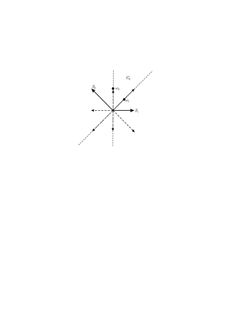
Figure 2: Root system of $B_{2}$ and fundamental weights.

Weyl orbit of a weight.

$(n_{1},n_{2})$ are coefficients in $\omega_{1}$, $\omega_{2}$ basis

$$(n_{1},n_{2}),\ \ (-n_{1},n_{1}+n_{2}),\ \ (n_{1}+2n_{2},-n_{2}),\ \ (-n_{1}-2n_{2},n_{1}+n_{2}),$$

$$(n_{1}+2n_{2},-n_{1}-n_{2}),\ \ (-n_{1}-2n_{2},n_{2}),\ \ (n_{1},-n_{1}-n_{2}),\ \ (-n_{1},-n_{2}).$$

Dimension of representation.

Weyl formula:

$$\dim V=\prod_{\alpha\in R}{\frac{\langle\lambda_{0}+\varrho,\alpha\rangle}{\langle\varrho,\alpha\rangle}},$$

where $\varrho=1/2\sum\limits_{\alpha\in R^{+}}\alpha=2\beta_{1}+3/2\beta_{2}$ and $\lambda_{0}$ is a dominant weight, i.e. the weight with non-negative integer coefficients in the basis of fundamental weights $\omega_{1,2}$, $\lambda_{0}=(n_{1}+n_{2})\beta_{1}+(n_{1}/2+n_{2})\beta_{2}$, $n_{1,2}\in\mathbb{N}_{0}$.

$$\dim V=\tfrac{1}{6}(n_{1}+1)(n_{2}+1)(n_{1}+2n_{2}+3)(n_{1}+n_{2}+2).$$

Eigenvalues of Casimir:

$$Q_{\lambda_{0}}(n_{1},n_{2})=-\tfrac{1}{2}\left(n_{1}^{2}+2n_{2}^{2}+2n_{1}n_{2}+4n_{1}+6n_{2}\right).$$ (A.1)

Weyl equivalence with UIR.

Two irreps are Weyl equivalent if they share same Casimir eigenvalue. Comparing (A.1) with (2.3) gives the possible solutions:

$$n_{1}=-2q,\qquad n_{2}=p+q-1,$$ (A.2)

$$n_{1}=2q-2,\qquad n_{2}=p-q,$$ (A.3)

$$n_{1}=q-1,\qquad n_{2}=-2p-2,$$

$$n_{1}=-2p-2,\qquad n_{2}=p-q.$$

Only (A.2) for $q=0$, $p\geq 1$, and (A.3) for $q\geq 1$, $p\geq 1$, yield possible Weyl equivalence between finite-dimensional irreps $(n_{1},n_{2})$ and UIR’s $\Pi_{p,q}^{\pm}$ in the discrete series.

Characters:

$$\xi=m_{1}\omega_{1}+m_{2}\omega_{2},$$

$$\chi_{n_{1},n_{2}}(m_{1},m_{2})=\frac{e^{\frac{1}{12}(-2m_{1}n_{1}-3m_{2}n_{1}-3m_{1}n_{2}-4m_{2}n_{2})}}{\big{(}-1+e^{m_{1}/12}\big{)}\big{(}-1+e^{m_{2}/6}\big{)}\big{(}-1+e^{\frac{m_{1}+m_{2}}{6}}\big{)}\big{(}-1+e^{\frac{1}{12}(m_{1}+2m_{2})}\big{)}}$$

$$\phantom{\chi_{n_{1},n_{2}}(m_{1},m_{2})=}{}\times\big{(}-e^{\frac{1}{12}((m_{1}+2m_{2})(3+2n_{1})+4m_{1}n_{2}+6m_{2}n_{2})}-e^{\frac{1}{12}(m_{1}+2(m_{1}+m_{2})(n_{1}+n_{2}))}$$

$$\phantom{\chi_{n_{1},n_{2}}(m_{1},m_{2})=}{}+e^{\frac{1}{12}(m_{1}+4m_{2}+2(m_{1}+2m_{2})(n_{1}+n_{2}))}+e^{\frac{1}{12}(2m_{2}(n_{1}+n_{2})+m_{1}(n_{1}+2n_{2}))}$$

$$\phantom{\chi_{n_{1},n_{2}}(m_{1},m_{2})=}{}+e^{\frac{1}{12}(3m_{1}+2m_{2}+2(m_{1}+m_{2})(n_{1}+2n_{2}))}-e^{\frac{1}{12}(2m_{2}+(m_{1}+2m_{2})(n_{1}+2n_{2}))}$$

$$\phantom{\chi_{n_{1},n_{2}}(m_{1},m_{2})=}{}+e^{\frac{1}{12}m_{1}(4+3n_{1}+4n_{2})}\big{(}-e^{\frac{1}{3}m_{2}(1+n_{1}+n_{2})}+e^{\frac{1}{6}m_{2}(3+2n_{1}+3n_{2})}\big{)}\big{)}.$$

Acknowledgements

P. Siegl appreciates the support of CTU grant No. CTU0910114 and MSMT project No. LC06002.

References

- [1]
- [2] Allen B., Vacuum states in de Sitter space, Phys. Rev. D 32 (1985), 3136–3149.
- [3] Allen B., Folacci A., Massless minimally coupled scalar field in de Sitter space, Phys. Rev. D 35 (1987), 3771–3778.
- [4] Bros J., Gazeau J.-P., Moschella U., Quantum field theory in the de Sitter universe, Phys. Rev. Lett. 73 (1994), 1746–1749.
- [5] Bros J., Epstein H., Moschella U., Analyticity properties and thermal effects for general quantum field theory on de Sitter space-time, Comm. Math. Phys. 196 (1998), 535–570, gr-qc/9801099.
- [6] Bros J., Moschella U., Two-point functions and quantum fields in de Sitter universe, Rev. Math. Phys. 8 (1996), 327–391, gr-qc/9511019.
- [7] Brunetti R., Guido D., Longo R., Modular localization and Wigner particles, Rev. Math. Phys. 14 (2002), 759–785, math-ph/0203021.
- [8] Caldwell R., Kamionkowski M., The physics of cosmic acceleration, Ann. Rev. Nucl. Part. Sci. 59 (2009), 397–429, arXiv:0903.0866.
- [9] Chernikov N.A., Tagirov E.A., Quantum theory of scalar fields in de Sitter space-time, Ann. Inst. H. Poincaré Sect. A (N.S.) 9 (1968), 109–141.
- [10] De Bièvre S., Renaud J., The massless quantum field on the 1+1-dimensional de Sitter space, Phys. Rev. D 57 (1998), 6230–6241.
- [11] Dixmier J., Représentations intégrables du groupe de De Sitter, Bull. Soc. Math. France 89 (1961), 9–41.
- [12] Fulling S.A., Aspects of quantum field theory in curved spacetime, London Mathematical Society Student Texts, Vol. 17, Cambridge University Press, Cambridge, 1989.
- [13] Garidi T., Huguet E., Renaud J., de Sitter waves and the zero curvature limit, Phys. Rev. D 67 (2003), 124028, 5 pages, gr-qc/0304031.
- [14] Gazeau J.-P., An introduction to quantum field theory in de Sitter space-time, in Cosmology and Gravitation: XIIth Brazilian School of Cosmology and Gravitation, AIP Conf. Proc., Vol. 910, Amer. Inst. Phys., Melville, NY, 2007, 218–269.
- [15] Gazeau J.-P., Novello M., The question of mass in (anti-) de Sitter spacetimes, J. Phys. A: Math. Theor. 41 (2008), 304008, 14 pages.
- [16] Gazeau J.-P., Renaud J., Takook M.V., Gupta–Bleuler quantization for minimally coupled scalar fields in de Sitter space, Classical Quantum Gravity 17 (2000), 1415–1434, gr-qc/9904023.
- [17] Gazeau J.-P., Youssef A., A discrete nonetheless remarkable brick in de Sitter: the “massless minimally coupled field”, in Proceedings of the XXVIIth International Colloquium on Group Theoretical Methods in Physics (Yerevan, 2008), Phys. Atomic Nuclei, to appear, arXiv:0901.1955.
- [18] Hua L.K., Harmonic analysis of functions of several complex variables in the classical domains, American Mathematical Society, Providence, R.I., 1963.
- [19] Isham C.J., Quantum field theory in curved space-times, a general mathematical framework, in Differential Geometrical Methods in Mathematical Physics II (Proc. Conf., Univ. Bonn, Bonn, 1977), Lecture Notes in Math., Vol. 676, Editors K. Bleuler et al., Springer, Berlin, 1978, 459–512.
- [20] Jakobczyk L., Strocchi F., Krein structures for Wightman and Schwinger functions, J. Math. Phys. 29 (1988), 1231–1235.
- [21] Kirsten K., Garriga J., Massless minimally coupled fields in de Sitter space: -symmetric states versus de Sitter-invariant vacuum, Phys. Rev. D 48 (1993), 567–577, gr-qc/9305013.
- [22] Linder E.V., Resource letter DEAU-1: dark energy and the accelerating universe, Amer. J. Phys. 76 (2008) 197–204, arXiv:0705.4102.
- [23] Magnus W., Oberhettinger F., Soni R.P., Formulas and theorems for the special functions of mathematical physics, Springer-Verlag, New York, 1966.
- [24] Mickelsson J., Niederle J., Contractions of representations of de Sitter groups, Comm. Math. Phys. 27 (1972), 167–180.
- [25] Morchio G., Pierotti D., Strocchi F., Infrared and vacuum structure in two-dimensional local quantum field theory models. The massless scalar field, J. Math. Phys. 31 (1990), 1467–1477.
- [26] Newton T.D., A note on the representations of the de Sitter group, Ann. of Math. (2) 51 (1950), 730–733.
- [27] Newton T.D., Wigner E.P., Localized states for elementary systems, Rev. Modern Phys. 21 (1949), 400–406.
- [28] Pinczon G., Simon J., Extensions of representations and cohomology, Rep. Math. Phys. 16 (1979), 49–77.
- [29] Schmidt H.J., On the de Sitter space-time – the geometric foundation of inflationary cosmology, Fortschr. Phys. 41 (1993), no. 3, 179–199.
- [30] Takahashi B., Sur les représentations unitaires des groupes de Lorentz généralisés, Bull. Soc. Math. France 91 (1963), 289–433.
- [31] Thomas L.H., On unitary representations of the group of de Sitter space, Ann. of Math. (2) 42 (1941), 113–126.
- [32] Wald R.M., Quantum fields theory in curved spacetime and black hole thermodynamics, Chicago Lectures in Physics, University of Chicago Press, Chicago, IL, 1994.