Università degli Studi di Catania
Scuola Superiore di Catania

Filippo Caruso

Storing Quantum Information
via Atomic Dark Resonances

diploma di licenza

Relatore:
	Chiar.mo Prof. F. S. Cataliotti

Anno Accademico 2004/2005

Introduction

It is now widely accepted that quantum mechanics allows for fundamentally new forms of communication and computation. Indeed recently many interesting new concepts in the field of quantum information such as quantum computation, quantum cryptography, quantum cloning and teleportation [1, 2, 3, 4] have left the theoretical domain to become commercial prototypes like quantum key distribution systems (QKD) [5]. In these protocols information is encoded in delicate quantum states, like the polarization state of single-photons, and subsequently it should be manipulated and transported [6] without being destroyed.

In this context on one hand atoms or similar systems like quantum dots represent reliable and long-lived storage and processing units. On the other hand photons are ideal carriers of quantum information [6, 7]: they are fast, robust but they are difficult to localize and process. Actually photons play a key role in network quantum computing [8], in long-distance, secure quantum communication and quantum teleportation [9, 10, 11, 12, 13]. As an example we can cite the application to teleportation which is of particular interest because of its potentials for quantum information processing with linear optical elements [14, 15]. Nevertheless, photons normally behave as non-interacting particles. This property ensures that information encoded in optical signals will be insensitive to environmental disturbances. For this reason optics has emerged as the preferred method for communicating information. In contrast, the processing of information requires interactions between signal carriers, that is, either between different photons or photons and electrons. Therefore one of the main challenges of nonlinear optical science is the “tailoring” of material properties to enhance such interactions, while minimizing the role of destructive processes such as photon absorption.

Therefore today’s challenge is to interface the photons to the atoms in order to realize a quantum network. One of the essential ingredients for this idea is a reliable quantum memory capable of a faithful storage and a prompt release of the quantum states of the photons. We need to develop a technique for coherent transfer of quantum information carried by light to atoms and vice versa and in order to achieve a unidirectional transfer (from field to atoms or vice versa) an explicit time dependent control mechanism is required.

Optical storage has been already investigated for classical data. Particularly interesting are techniques based on Raman photon echos [16] as they combine the long lifetime of ground-state hyperfine or Zeeman coherences for storage with data transfer by light at optical frequencies [17]. Nevertheless, while these techniques are very powerful for high-capacity storage of classical optical data, they cannot be used for quantum memory purposes; indeed they employ direct or dressed-state optical pumping and thus contain dissipative elements or have other limitations in the transfer process between light and matter. As a consequence they do not operate on the level of individual photons and cannot be applied to quantum information processes.

The conceptually simplest approach to a quantum memory for light is to “store” the state of a single photon in an individual atom. This approach involves a coherent absorption and emission of single photons by single atoms and it is very inefficient because the single-atom absorption cross-section is very small. A very elegant solution to this problem is provided by cavity QED [18]. Indeed placing an atom in a high-$Q$ resonator effectively enhances its cross-section by the number of photon round-trips during the ring-down time and thus makes an effective transfer possible [19]. Raman adiabatic passage techniques [20] with time-dependent external control fields can be used to implement a directed but reversible transfer of the quantum state of a photon to the atom (i.e. coherent absorption). However, despite the enormous experimental progress in this field [21], it is technically very challenging to achieve the necessary strong-coupling regime. In addition the single-atom system is by construction highly susceptible to the loss of atoms and the speed of operations is limited by the large $Q$-factor. On the other hand if atomic ensembles are used rather than individual atoms no such requirements exists and coherent and reversible transfer techniques for individual photon wavepackets [22, 23, 24, 25, 26, 27, 28] and cw light fields [29, 30, 31, 32] have been proposed and in part experimentally implemented.

Recently the authors in [23, 24, 33] have proposed a technique based on an adiabatic transfer of the quantum state of photons to collective atomic excitations (dark–state polaritons, DSP) using electromagnetically induced transparency (EIT) in three–level atomic schemes [34].

In this thesis we investigate how to obtain a quantum memory of a coherent state with atomic systems and we point out that it is possible to compensate the unavoidable losses using the amplification without inversion in the EIT regime. For this aim we analyze in detail the propagation of a coherent light pulse through a medium under the conditions for gain without inversion. Moreover we introduce a quantum memory for polarized photons with a four–level system and investigate the scattering of dark–state polaritons in a tripod configuration.

The layout of this thesis is as follows.

Chapter 1 shows a brief review of some concepts of Quantum Optics and, in particular, the essence of the electromagnetically induced transparency. We analyze a three–level system, interacting with two laser fields, in which destructive quantum interference appears and no atomic population is promoted to the excited states, leading to a vanishing light absorption. In these conditions, the narrow transparency resonance is accompanied by a very steep variation of the refractive index with frequency and therefore a strong variation of the group velocity in light propagation in an EIT medium. Then we summarize some results of classical electromagnetic theory and from the Scroedinger equation we derive expressions for density matrix, i.e. optical Bloch equations, and for the expression for the susceptibility.

Chapter 2 is devoted entirely to the propagation of a gaussian pulse along a cigar-shaped cloud of atoms in EIT regime; we derive expressions for the group velocity and we calculate the expectation value after transmission of the probe pulse normal-order Poynting vector. When the central frequency of the pulse is resonant with an atomic transition, we show that it is possible to amplify a slow propagating pulse without population inversion. We also analyze the regime of anomalous light propagation showing that it is possible to observe superluminal energy propagation. Particularly we show these results for both cold and hot atoms. In this last case we analyze a realistic system in a 10 cm long cell containing ⁸⁷Rb at a temperature of $35^{\circ}$C and with a density equal to $5.296\cdot 10^{7}$ $atoms/cm^{3}$.

Chapter 3 discusses how to imprint the information carried by the photons onto the atoms, specifically as a coherent pattern of atomic spins. The procedure is reversible and the information stored in the atomic spins can later be transferred back to the light field, reconstituting the original pulse. Therefore we analyze the propagation of a quantum field in an EIT medium sustaining “dark state polaritons” in a quasi-particle picture. Moreover we study the decoherence effects in this quantum memory for photons, by analyzing the fidelity of the quantum state transfer.

Chapter 4 discusses the emergence of parastatistics in the quasi-particle picture in gain medium. Indeed the dark–state polaritons obey generalized bosons commutation relations that describe the mapping from bosons to fermions during the stopping of light and vice verse in the release. A deformation boson scheme is connected to this mapping and the Pauli principle is described by an effective repulsive interaction between the dark–state polaritons.

Chapter 5 introduces a polarization quantum memory for photons by using a tripod atomic configuration in which two ideal EIT windows appear. Therefore we study the scattering of two dark–state polaritons (DSP) and we show that they present a solitonic behavior.

In Appendix A.1 we show an application of EIT effect, based on the possibility to lase without population inversion (LWI). Afterwards we emphasize the concept of lasing without inversion through an original approach; indeed, reviewing the Einstein theory about light-matter interaction, there is a important relation between the possibility of lasing without inversion and a symmetry breaking between the Einstein B coefficients. In Appendix A.2 we discuss causality in the regime of anomalous light propagation showing that no contradiction is present. In Appendix A.3 we recall an important concept of the quantum information theory, the fidelity, and finally in Appendix A.4 we show the proof of No-Cloning Theorem.

Chapter 1 Dark resonance in three–level atomic systems

1.1 The story of the “three–level system”

Three–level systems have been the object of extensive studies, both theoretically and experimentally, for the past thirty years. The reason for this prolonged interest must be searched in the fact that a three–level system is the test model for quantum interference effects to appear on a macroscopic scale. The possibility of completely changing the absorptive and dispersive characteristic of a medium at a given frequency by applying a coherent field at a different frequency is both intriguing and surprising.

As early as 1933 Weisskopf [35] used a three–level model to predict spectral narrowing and frequency shift of resonant fluorescence due to narrow-band optical pumping. No experimental confirmation was possible at that time given the absence of a narrow-band spectral source. In 1955 Autler and Townes [36] demonstrated that in presence of a strong coupling microwave field the resonant absorption of a probe field coupled to a different transition was split into a doublet (AC Stark splitting or Autler-Townes effect) [see Sec. 1.3].

In 1976 in Pisa, the group of A. Gozzini [37] observed a sudden drop of fluorescence in a sodium vapor where a three–level system with two ground and an excited level was irradiated by two modes of a dye laser. In the sodium cell an inhomogeneous magnetic field was applied almost along the laser propagation axis and the fluorescence drop appeared as a dark line in the fluorescent image. The effect was soon recognized to be due to optical pumping of atoms in a coherent superposition of the two ground states which was uncoupled from the laser light (Coherent Population Trapping (CPT) or Dark resonance) [38, 39]. The same effect was independently investigated first theoretically in a system where the three levels were arranged in cascade by Whitley and Stroud [40] then experimentally once again in sodium in a system with two ground and one excited level by Gray, Whitley and Stroud [41]. In the last eighties the Velocity Selective Coherent Population Trapping (VSCPT) [42] method took advantage of dark resonance to cool and trap atoms below the one-photon-recoil limit. Renewed interest was brought into the field in the same years when it was recognized that three–levels systems could provide amplification and eventually lasing without population inversion (AWI, LWI). In 1991 Harris [34] called “Electromagnetically Induced Transparency” (EIT) [43] the interference effect leading to a reduction in absorption in the center of an Autler-Townes doublet.

Today this physical system is at the basis of all the recent experiments on slow light propagation [44, 25, 26] and speculations about possible realizations of quantum memories [27], quantum phase gates [45] and photon–counters with unprecedented efficiency [46, 28].

1.2 EIT domain

Electromagnetically induced transparency (EIT) is a quantum interference effect that permits the propagation of light through an otherwise opaque atomic medium; a “coupling” laser is used to create the interference necessary to allow the transmission of resonant probe pulses.

In general let us recall that the strength of the interaction between light and atoms is a function of the wavelength or frequency of light. When the light frequency matches the frequency of a particular atomic transition, a resonance condition occurs and the optical response of the medium is greatly enhanced. Light propagation is then accompanied by strong absorption and dispersion, as the atoms are actively promoted into fluorescing excited states. [47]

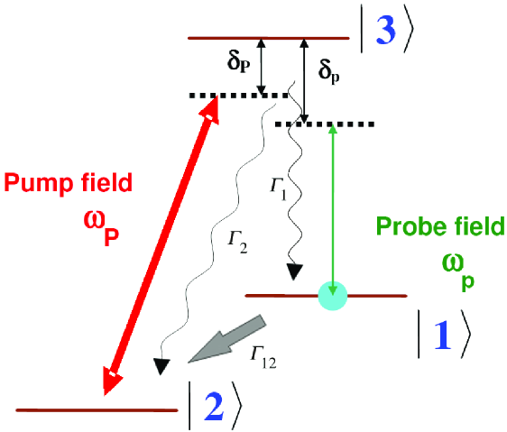
Figure 1.1: The three–level system interacting with two laser fields ($\Lambda$–configuration).

In order to understand in detail EIT effect, let us consider the situation in which the atoms have a pair of lower energy states ($|1\rangle$ and $|2\rangle$ in Fig. 1.1) in each of which the atoms can live for a long time. Such is the case for sublevels of different angular momentum (spin) within the electronic ground state of alkali atoms. In order to modify the propagation through this atomic medium of a light field (probe field) that couples the ground state $|1\rangle$ to an electronically excited state $|3\rangle$, one can apply a second “control” field (pump field) that is quasi resonant with the transition $|3\rangle\leftrightarrow|2\rangle$. Particularly in the scheme shown in Fig. 1.1 the states $\left.|3\right\rangle$ and $\left.|1\right\rangle$ are coupled by a weak probe beam at frequency $\omega_{p}$ while a stronger pump beam at frequency $\omega_{P}$ couples the states $\left.|2\right\rangle$ and $\left.|3\right\rangle$.

Such a system exhibits a new set of coherent phenomena mainly correlated with population trapping and quantum interference. For any combination of intensities of the two fields, there will be superpositions of the atomic states, $|1\rangle$ and $|2\rangle$, that is in counterphase with the field, such combination can not absorb light and is therefore called dark state (there is also an in-phase component which is named bright state). In other terms, the two possible pathways in which light can be absorbed by atoms ($|1\rangle\mapsto|3\rangle$ and $|2\rangle\mapsto|3\rangle$) can interfere and cancel each other. With such destructive quantum interference, none of the atoms are promoted to the excited states, leading to a vanishing light absorption.

From the theoretical point of view it is possible to write the free-Hamiltonian $\hat{H}_{0}$ and the atom-laser interaction Hamiltonian $\hat{H}_{I}$ as follows:

$$\hat{H_{0}}=\sum_{j=1}^{3}\hbar\omega_{j}|j\rangle\langle j|+\hbar\omega_{p}\hat{a}_{p}^{\dagger}\hat{a}_{p}+\hbar\omega_{P}\hat{a}_{P}^{\dagger}\hat{a}_{P}$$ (1.1)

$$\hat{H}_{I}=\hbar g_{p}\hat{a}_{p}|3\rangle\langle 1|+\hbar g_{P}\hat{a}_{P}|3\rangle\langle 2|+h.c.$$ (1.2)

where $\hat{a}$ and $\hat{a}^{\dagger}$ are the annihilation and creation operators for the two fields and $g$ are the relative coupling coefficients as shown in Sec. 1.5.

Now, let us consider the following two orthogonal linear combinations of the lower states ($|1\rangle$, $|2\rangle$):

$$|C\rangle=\frac{1}{(\Omega_{p}^{2}+\Omega_{P}^{2})^{1/2}}(\Omega_{p}|1\rangle+\Omega_{P}|2\rangle)$$ (1.3)

$$|NC\rangle=\frac{1}{(\Omega_{p}^{2}+\Omega_{P}^{2})^{1/2}}(\Omega_{P}|1\rangle-\Omega_{p}|2\rangle)$$ (1.4)

where $\Omega_{p}$ and $\Omega_{P}$ are coefficients proportional, respectively, to $\hbar g_{p}\langle\hat{a}_{p}\rangle$ and $\hbar g_{P}\langle\hat{a}_{P}\rangle$.

This defines the uncoupled and coupled states which have the property that, according to the atom-laser interaction Hamiltonian of Eq. (1.2), the transition matrix element between $|NC\rangle$ and $|3\rangle$ vanishes:

$$\langle 3|\hat{H}_{I}|NC\rangle=0$$ (1.5)

whereas

$$\langle 3|\hat{H}_{I}|C\rangle\neq 0$$ (1.6)

Consequently, an atom in the uncoupled state $|NC\rangle$ cannot absorb photons and cannot be excited to $|3\rangle$. Moreover for an atom prepared in the $|NC\rangle$ state, the Scroedinger equation under the Hamiltonian $\hat{H}_{0}+\hat{H}_{I}$ results in:

$$\frac{d}{dt}|NC\rangle=\frac{1}{i\hbar}(\hat{H}_{0}+\hat{H}_{I})|NC\rangle=0$$ (1.7)

Thus an atom prepared in $|NC\rangle$ remains in this state and can leave it neither by the free evolution (effect of the free Hamiltonian $\hat{H}_{0}$) nor by absorption of a laser photon (effect of the atom-laser interaction $\hat{H}_{I}$). Besides, because $|NC\rangle$ is a linear combination of the two ground states, and is radiatively stable, the atom cannot leave $|NC\rangle$ either by spontaneous emission. This is the essence of the riga nera [37] (dark resonance) or electromagnetically induced transparency (EIT).

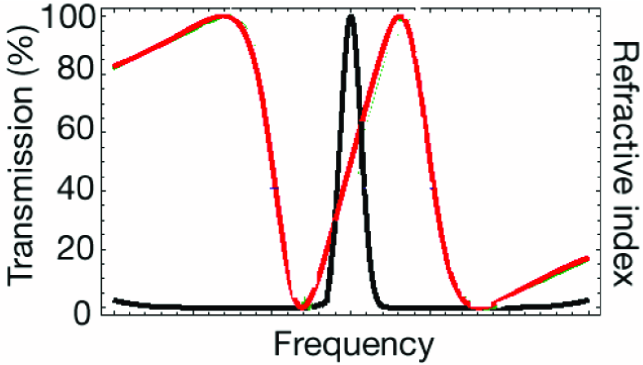
Figure 1.2: Spectrum of transmission and refractive index corresponding to EIT. Rapid variation of the refractive index (red curve) causes a reduction of group velocity. [44]

The reduction in the probe absorption can also be explained [34, 39] as due to a combination of AC-Stark splitting (see Sec. 1.3) and destructive quantum interference in the absorption of a probe photon from the two coherent superpositions of lower states to the excited state $\left.|3\right\rangle$. This interference is analogous to that seen if mutually coherent optical fields are interfered such as in the common Young interferometer. Yet another way to view this effect is in terms of the creation of a new class of laser dressed matter in which laser fields and atoms have become strongly coupled.

1.3 AC-Stark Effect

In general when the laser is resonant with an atomic transition two effects come into play: the Rabi oscillations and the AC Stark Effect or Autler-Townes Doublet [36].

First of all, because of coupling laser, the electrons cycle back and forth between the two levels: these are the Rabi oscillations and their characteristic frequency is the so–called Rabi frequency.

Due to this rapid oscillation the atom acquires an induced electric dipole that interacts with the laser electric field splitting both the upper and the lower level of the transition into two sub levels - one higher in energy the other lower. This splitting of the energy levels is caused by the oscillating electric field of the laser beam [48]: it is the AC Stark effect.

Both of these effects are dependent on the generalized Rabi frequency ($\Omega$) that gives us information concerning how effectively the laser can stimulate transitions in the atom and it is dependent on:

• Laser field strength ($\vec{E}$)

• Dipole moment of the transition ($\vec{\mu}$)

• Difference between the laser and the atomic transition frequencies, i.e. detuning($\delta$).

It is defined as:

$$\Omega_{R}=\sqrt{\left(\frac{\vec{\mu}\cdot\vec{E}}{\hbar}\right)^{2}+\delta^{2}}$$ (1.8)

The new levels are separated by $\Omega_{R}$ and with a population dependent on the laser detuning.

1.4 Macroscopic theory of absorption

Before considering the density-matrix approach to the three–level system, it is convenient to summarize the relevant results of classical electromagnetic theory [49]. Let us analyze a gas of atoms in a cavity as a dielectric medium: the presence of this dielectric leads to the generation of a polarization P by an applied electric field E. By definition, the polarization is equal to:

$$\textbf{P}=\frac{N}{V}\ \textbf{d}$$ (1.9)

where $\frac{N}{V}$ is the atomic density and d is the electric dipole moment. For electric fields that are not too strong, the polarization is proportional to the field,

$$\textbf{P}=\varepsilon_{0}\chi\textbf{E}$$ (1.10)

where $\chi$ is the linear electric susceptibility and $\varepsilon_{0}$ is the vacuum electric permittivity. The susceptibility is a function of the frequency $\omega$ of the applied field, whose form depends on the energy levels and wave functions of the atoms that make up the dielectric. Maxwell’s equations still have wavelike solutions, but the relation between frequency, $\omega$, and wavevector, $k$, has the following general expression:

$$\Big{(}\frac{kc}{\omega}\Big{)}^{2}=1+\chi$$ (1.11)

which reduces to known dispersion equation $\omega=kc$ in the free-space limit $\chi=0$; $c$ is the velocity of light in vacuum.

The quantity $1+\chi$ is known as the dielectric constant; of course, it is constant only in the sense of being independent of E but its magnitude is a function of the frequency. Moreover, the susceptibility is generally a complex quantity and we write

$$\chi=\chi^{\prime}+i\chi^{\prime\prime}$$ (1.12)

where $\chi^{\prime}$ and $\chi^{\prime\prime}$ are, respectively, the real and imaginary parts of $\chi$.

It is conventional to write the square root of Eq. (1.11) as

$$\frac{kc}{\omega}=\eta+i\kappa$$ (1.13)

where $\eta$ and $\kappa$, so defined, are, respectively, the refractive index and extinction coefficient. Comparison of the real and imaginary parts of Eq. (1.11) after substitution of Eq. (1.13) yields

$$\eta^{2}-\kappa^{2}=1+\chi^{\prime}$$

$$2\eta\kappa=\chi^{\prime\prime}$$ (1.14)

These equations will be used to determine the frequency dependence of $\eta$ and $\kappa$ once the frequency-dependent susceptibility is knows through a off-diagonal term of the density operator.

1.5 The Optical Bloch Equations (OBE)

Let us investigate in detail the scheme shown in Fig. 1.1. A generic atomic state can be written as a linear superposition of the atomic eigenstates

$$|\psi\rangle=C_{1}|1\rangle+C_{2}|2\rangle+C_{3}|3\rangle$$ (1.15)

and the density matrix operator, $\hat{\rho}$, is given by the outer product of two wave functions,

$$\hat{\rho}=|\psi\rangle\langle\psi|\Longrightarrow\left(\begin{array}[]{ccc}|C_{1}|^{2}&C_{1}C_{2}^{*}&C_{1}C_{3}^{*}\\ C_{2}C_{1}^{*}&|C_{2}|^{2}&C_{2}C_{3}^{*}\\ C_{3}C_{1}^{*}&C_{3}C_{2}^{*}&|C_{3}|^{2}\end{array}\right)=\left(\begin{array}[]{ccc}\rho_{11}&\rho_{12}&\rho_{13}\\ \rho_{21}&\rho_{22}&\rho_{23}\\ \rho_{31}&\rho_{32}&\rho_{33}\end{array}\right)$$

The diagonal terms give us the probability of finding the atom in one of the three levels while the transverse terms are proportional to the complex dipole moments. The off-diagonal elements are generally complex and they satisfy the following relations:

$$\rho_{21}=\rho_{12}^{*}\ \ \ \ \ \ \ \rho_{13}=\rho_{31}^{*}\ \ \ \ \ \ \ \rho_{23}=\rho_{32}^{*}$$ (1.16)

The expectation value of any operator ($\hat{A}$) can now be written in terms of $\rho$ as

$$\langle\hat{A}\rangle=Tr(\hat{A}\hat{\rho})=\sum_{i,j=1}^{3}\rho_{ij}A_{ij}$$ (1.17)

In our case, the hamiltonian operator of the three–level system is the following one:

$$\hat{H}=\hat{H_{0}}+\hat{H_{I}}$$

where the free- and interaction-hamiltonian are

$$\hat{H_{0}}=\sum_{j=1}^{3}\hbar\omega_{j}|j\rangle\langle j|+\hbar\omega_{p}\hat{a}_{p}^{\dagger}\hat{a}_{p}+\hbar\omega_{P}\hat{a}_{P}^{\dagger}\hat{a}_{P}$$ (1.18)

$$\hat{H}_{I}=\hbar g_{p}\hat{a}_{p}|3\rangle\langle 1|+\hbar g_{P}\hat{a}_{P}|3\rangle\langle 2|+h.c.$$ (1.19)

where the notation is the same as in Sec. 1.2.

Making a transformation to a rotating frame and performing the rotating wave approximation (RWA), which consists in neglecting the antiresonant term containing the sum frequency and therefore very rapidly oscillating, we obtain

$$\tilde{H}=\sum_{j=1}^{3}\hbar\omega_{j}|j\rangle\langle j|+(\hbar g_{p}e^{-i\omega_{p}t}\hat{a}_{p}|3\rangle\langle 1|+\hbar g_{P}e^{-i\omega_{P}t}\hat{a}_{P}|3\rangle\langle 2|+h.c.)$$

Note that the approximation is justified because the effect of the terms that oscillate at frequency $\omega_{p}+\omega_{P}$ is negligible compared to the effect of the terms that oscillate at frequency $\omega_{p}-\omega_{P}$ when $\omega_{P}$ is close to $\omega_{p}$.

For a set of classical fields (i.e. coherent states), we have

$$\hbar g_{p}\hat{a}_{p}\longrightarrow\hbar g_{p}\langle\hat{a}_{p}\rangle\equiv-\frac{\hbar}{2}\Omega_{p}e^{-i\phi_{p}}=\vec{p}_{31}\cdot\vec{E}=e\langle 3|\vec{x}|1\rangle\cdot\widehat{\epsilon}_{p}\ \epsilon_{p}$$ (1.20)

$$\hbar g_{P}\hat{a}_{P}\longrightarrow\hbar g_{P}\langle\hat{a}_{P}\rangle\equiv-\frac{\hbar}{2}\Omega_{P}e^{-i\phi_{P}}=\vec{p}_{32}\cdot\vec{E}=e\langle 3|\vec{x}|2\rangle\cdot\widehat{\epsilon}_{P}\ \epsilon_{P}$$ (1.21)

where $\vec{p}$ is the transition dipole moment, $\Omega_{p}$ and $\Omega_{P}$ are the Rabi frequencies (real), $\phi_{p}$ and $\phi_{P}$ are the relative phases, $e$ is the electron charge, $\widehat{\epsilon}_{p}$ and $\widehat{\epsilon}_{P}$ are the unit polarization vector and $\epsilon_{p}$ and $\epsilon_{P}$ are the electric field amplitudes. Then the hamiltonian operator is

$$\tilde{H}=\sum_{j=1}^{3}\hbar\omega_{j}|j\rangle\langle j|+\{-\frac{\hbar}{2}\Omega_{p}e^{-i\phi_{p}}e^{-i\omega_{p}t}|3\rangle\langle 1|-\frac{\hbar}{2}\Omega_{P}e^{-i\phi_{P}}e^{-i\omega_{P}t}|3\rangle\langle 2|+h.c.\}$$

In order to find the equation of motion for the density matrix elements, $\rho_{ij}$, starting from the Schrödinger equation, we consider the Liouville equation for $\rho$:

$$\dot{\hat{\rho}}=-\frac{i}{\hbar}[\tilde{H},\hat{\rho}]-\dot{\hat{\rho}}_{int}-\dot{\hat{\rho}}_{ext}$$ (1.22)

Generally it is possible to divide relaxation phenomena into two groups: in the first one the system relaxes towards external states $\dot{\hat{\rho}}_{ext}$ (external relaxation) and in the second one it relaxes towards internal states $\dot{\hat{\rho}}_{int}$ (internal relaxation). These rates are given by

$$\dot{\hat{\rho}}^{i\longrightarrow j}_{int}=-\frac{T_{ij}}{2}\{\left.|i\right\rangle\left\langle i|\right.,\hat{\rho}\}+T_{ij}\rho_{ii}\left.|j\right\rangle\left\langle j|\right.$$ (1.23)

$$\dot{\hat{\rho}}_{ext}=\frac{1}{2}\Big{\{}\sum_{i}{\zeta_{i}\left.|i\right\rangle\left\langle i|\right.},\hat{\rho}\Big{\}}$$ (1.24)

where $T_{ij}$ and $\zeta_{i}$ are, respectively, the internal and external decay rates; $\dot{\rho}^{i\longrightarrow j}_{int}$ represents the internal decay from level $\left.|i\right\rangle$ into level $\left.|j\right\rangle$. Note that in Fig. 1.1 we have $\Gamma_{1}=T_{31}$, $\Gamma_{2}=T_{32}$ and $\Gamma_{12}=T_{12}$ and we neglect the external decays. Actually there is no decay between two lower-states because they are meta-stable but we introduce an incoherent RF field that simulates a loss from $\left.|1\right\rangle$ and places population back into $\left.|2\right\rangle$ (as it will be clear in Sec. 2.7).

By treating this three–level system as closed, the equations of motion for the density matrix elements, $\rho_{ij}$, are:

$$\dot{\rho}_{31} = -[\frac{1}{2}(\Gamma_{1}+\Gamma_{2}+\Gamma_{12})+i\omega_{31}]\rho_{31}+\frac{i}{2}\Omega_{P}e^{-i\phi_{P}}e^{-i\omega_{P}t}\rho_{21}+$$

$$-\frac{i}{2}\Omega_{p}e^{-i\phi_{p}}e^{-i\omega_{p}t}(\rho_{33}-\rho_{11})$$

$$\dot{\rho}_{32} = -[\frac{1}{2}(\Gamma_{1}+\Gamma_{2})+i\omega_{32}]\rho_{32}+\frac{i}{2}\Omega_{p}e^{-i\phi_{p}}e^{-i\omega_{p}t}\rho_{12}+$$ (1.25)

$$-\frac{i}{2}\Omega_{P}e^{-i\phi_{P}}e^{-i\omega_{P}t}(\rho_{33}-\rho_{22})\ \ \ \ \ \ \ \ \$$

$$\dot{\rho}_{21} = -[\Gamma_{12}+i\omega_{21}]\rho_{21}+\frac{i}{2}\Omega_{P}e^{-i\phi_{P}}e^{-i\omega_{P}t}\rho_{31}-\frac{i}{2}\Omega_{p}e^{-i\phi_{p}}e^{-i\omega_{p}t}\rho_{23}$$

$$\dot{\rho}_{33} = (\frac{i}{2}\Omega_{p}e^{-i\phi_{p}}e^{-i\omega_{p}t}\rho_{13}+\frac{i}{2}\Omega_{P}e^{-i\phi_{P}}e^{-i\omega_{P}t}\rho_{23}+h.c.)-(\Gamma_{1}+\Gamma_{2})\rho_{33}$$

$$\dot{\rho}_{22} = (-\frac{i}{2}\Omega_{P}e^{-i\phi_{P}}e^{-i\omega_{P}t}\rho_{23}+h.c.)+\Gamma_{2}\rho_{33}+\Gamma_{12}\rho_{11}$$

$$\dot{\rho}_{11} = -\dot{\rho}_{22}-\dot{\rho}_{33}$$

These are known as Optical Bloch Equations (OBE). They are similar to equations derived by Bloch to describe the motion of a spin in an oscillatory magnetic field. The quantum mechanics of the three–level atom considered here is formally identical to that of a spin $1$ system. Indeed it is possible to draw many analogies between the influences of oscillatory fields on the two systems.

These equations can be solved without any further approximations. They represent a set of six simultaneous equations for the six independent elements of the atomic density matrix. After obtaining the steady state solution, we will be able to use the off-diagonals terms to calculate the susceptibility and therefore the frequency dependence of the refractive index and extinction coefficient; after these analytical calculations, it is possible to analyze in detail CPT (coherent population trapping) and EIT effects.

Let us now introduce the slowly varying variables: ($\Delta_{1}^{{}^{\prime}}$, $\Delta_{2}^{{}^{\prime}}$, $\Delta_{3}^{{}^{\prime}}$ $\longrightarrow$ free parameters)

$$\rho_{31}\equiv e^{i\Delta_{1}^{{}^{\prime}}t}\tilde{\rho}_{31}\ \ \ \ \ \rho_{32}\equiv e^{i\Delta_{2}^{{}^{\prime}}t}\tilde{\rho}_{32}\ \ \ \ \ \rho_{21}\equiv e^{i\Delta_{3}^{{}^{\prime}}t}\tilde{\rho}_{21}\ \ \ \ \$$ (1.26)

and so we can rewrite the optical Bloch equations as:

$$\dot{\tilde{\rho}}_{31} = -\tilde{\rho}_{31}[\frac{1}{2}(\Gamma_{1}+\Gamma_{2}+\Gamma_{12})+i\Delta_{1}^{{}^{\prime}}+i\omega_{31}]+\frac{i}{2}\Omega_{P}e^{-i\phi_{P}-i\omega_{P}t-i\Delta_{1}^{{}^{\prime}}t+i\Delta_{3}^{{}^{\prime}}t}\tilde{\rho}_{21}+$$

$$-\frac{i}{2}\Omega_{p}e^{-i\phi_{p}-i\omega_{p}t-i\Delta_{1}^{{}^{\prime}}t}(\rho_{33}-\rho_{11})$$

$$\dot{\tilde{\rho}}_{32} = -\tilde{\rho}_{32}[\frac{1}{2}(\Gamma_{1}+\Gamma_{2})+i\Delta_{2}^{{}^{\prime}}+i\omega_{32}]+\frac{i}{2}\Omega_{p}e^{-i\phi_{p}-i\omega_{p}t-i\Delta_{2}^{{}^{\prime}}t-i\Delta_{3}^{{}^{\prime}}t}\tilde{\rho}_{12}+$$ (1.27)

$$-\frac{i}{2}\Omega_{P}e^{-i\phi_{P}-i\omega_{P}t-i\Delta_{2}^{{}^{\prime}}t}(\rho_{33}-\rho_{22})$$

$$\dot{\tilde{\rho}}_{21} = -\tilde{\rho}_{21}[\Gamma_{12}+i\Delta_{3}^{{}^{\prime}}+i\omega_{21}]+\frac{i}{2}\Omega_{P}e^{i\phi_{P}+i\omega_{P}t-i\Delta_{3}^{{}^{\prime}}t+i\Delta_{1}^{{}^{\prime}}t}\tilde{\rho}_{31}+$$

$$-\frac{i}{2}\Omega_{p}e^{-i\phi_{p}-i\omega_{p}t-i\Delta_{3}^{{}^{\prime}}t-i\Delta_{2}^{{}^{\prime}}t}\tilde{\rho}_{23}$$

$$\dot{{\rho}}_{33} = (\frac{i}{2}\Omega_{p}e^{-i\phi_{p}-i\omega_{p}t-i\Delta_{1}^{{}^{\prime}}t}\tilde{\rho}_{13}+\frac{i}{2}\Omega_{P}e^{-i\phi_{P}-i\omega_{P}t-i\Delta_{2}^{{}^{\prime}}t}\tilde{\rho}_{23}+h.c.)-(\Gamma_{1}+\Gamma_{2})\rho_{33}$$

$$\dot{\rho}_{22} = (-\frac{i}{2}\Omega_{P}e^{-i\phi_{P}-i\omega_{P}t-i\Delta_{2}^{{}^{\prime}}t}\tilde{\rho}_{23}+h.c.)+\Gamma_{2}\rho_{33}+\Gamma_{12}\rho_{11}$$

$$\dot{\rho}_{11} = -\dot{\rho}_{22}-\dot{\rho}_{33}$$

The three free frequency parameters $\Delta^{{}^{\prime}}$ can be chosen to eliminate the oscillating exponentials:

$$\Delta_{1}^{{}^{\prime}}=-\omega_{p}\ \ \ \ \Delta_{2}^{{}^{\prime}}=-\omega_{P}\ \ \ \ \ \Delta_{3}^{{}^{\prime}}=\omega_{P}+\Delta_{1}^{{}^{\prime}}=\omega_{P}-\omega_{p}$$ (1.28)

and therefore one obtains:

$$\dot{\tilde{\rho}}_{31} = -(\gamma_{1}+\gamma_{3}+i\delta_{p})\tilde{\rho}_{31}+\frac{i}{2}\Omega_{P}e^{-i\phi_{P}}\tilde{\rho}_{21}-\frac{i}{2}\Omega_{p}e^{-i\phi_{p}}(\rho_{33}-\rho_{11})$$

$$\dot{\tilde{\rho}}_{32} = -(\gamma_{3}+i\delta_{P})\tilde{\rho}_{32}+\frac{i}{2}\Omega_{p}e^{-i\phi_{p}}\tilde{\rho}_{12}-\frac{i}{2}\Omega_{P}e^{-i\phi_{P}}(\rho_{33}-\rho_{22})$$

$$\dot{\tilde{\rho}}_{21} = -(\gamma_{1}+i\delta)\tilde{\rho}_{21}+\frac{i}{2}\Omega_{P}e^{-i\phi_{P}}\tilde{\rho}_{31}-\frac{i}{2}\Omega_{p}e^{-i\phi_{p}}\tilde{\rho}_{23}$$ (1.29)

$$\dot{\tilde{\rho}}_{33} = (\frac{i}{2}\Omega_{p}e^{-i\phi_{p}}\tilde{\rho}_{13}+\frac{i}{2}\Omega_{P}e^{-i\phi_{P}}\tilde{\rho}_{23}+h.c.)-2\gamma_{3}\rho_{33}$$

$$\dot{\tilde{\rho}}_{22} = (-\frac{i}{2}\Omega_{P}e^{-i\phi_{P}}\tilde{\rho}_{23}+h.c.)+\Gamma_{2}\rho_{33}+2\gamma_{1}\rho_{11}$$

$$\dot{\rho}_{11} = -\dot{\rho}_{22}-\dot{\rho}_{33}$$

where the detunings are

$$\delta_{p}=\omega_{31}-\omega_{p}\ \ \ \ \delta_{P}=\omega_{32}-\omega_{P}\ \ \ \ \delta=\omega_{21}+\omega_{P}-\omega_{p}=\delta_{p}-\delta_{P}$$

and $\gamma_{3}\equiv\frac{1}{2}(\Gamma_{1}+\Gamma_{2})$, $\gamma_{1}\equiv\frac{\Gamma_{12}}{2}$.

We calculate the steady-state solution for $\tilde{\rho}_{31}$, after fixing the populations (unsaturated-populations solution, see Sec. 1.6).
We obtain:

$$\dot{\tilde{\rho}}_{32}=0\ \ \text{yields}\ \ \tilde{\rho}_{32} = \frac{i\Omega_{p}e^{-i\phi_{p}}}{2(\gamma_{3}+i\delta_{P})}\tilde{\rho}_{12}-\frac{i\Omega_{P}e^{-i\phi_{P}}}{2(\gamma_{3}+i\delta_{P})}(\rho_{33}-\rho_{22})$$

$$\ \ \ \ \ \ \ \ \ \ \ \ \tilde{\rho}_{23} = \frac{-i\Omega_{p}e^{i\phi_{p}}}{2(\gamma_{3}-i\delta_{P})}\tilde{\rho}_{21}+\frac{i\Omega_{P}e^{i\phi_{P}}}{2(\gamma_{3}-i\delta_{P})}(\rho_{33}-\rho_{22})$$

$$\dot{\tilde{\rho}}_{21}=0\ \ \text{yields}\ \ \tilde{\rho}_{21} = \frac{i\Omega_{P}e^{i\phi_{P}}}{2(\gamma_{1}+i\delta)}\tilde{\rho}_{31}-\frac{i\Omega_{p}e^{-i\phi_{p}}}{2(\gamma_{1}+i\delta)}\tilde{\rho}_{23}\ \ \ \ \ \ \ \ \ \ \ \ \ \$$

$$\dot{\tilde{\rho}}_{31}=0\ \ \text{yields}\ \ \tilde{\rho}_{31} = \frac{i\Omega_{P}e^{-i\phi_{P}}}{2(\gamma_{1}+\gamma_{3}+i\delta_{p})}\tilde{\rho}_{21}-\frac{i\Omega_{p}e^{-i\phi_{p}}}{2(\gamma_{1}+\gamma_{3}+i\delta_{p})}(\rho_{33}-\rho_{11})\ \$$

If we put $\tilde{\rho}_{21}$ back in $\tilde{\rho}_{31}$, we get:

$$\tilde{\rho}_{31}=-\frac{\frac{i\Omega_{p}e^{-i\phi_{p}}}{2(\gamma_{1}+\gamma_{3}+i\delta_{p}))}}{1+\frac{\Omega_{P}^{2}(\gamma_{3}-i\delta_{P})}{(\gamma_{1}+\gamma_{3}+i\delta_{p})\Big{(}4(\gamma_{3}-i\delta_{P})(\gamma_{1}+i\delta)+\Omega_{p}^{2}\Big{)}}}\Bigg{\{}(\rho_{33}-\rho_{11})-$$ (1.30)

$$-\frac{\Omega_{P}^{2}}{4(\gamma_{3}-i\delta_{P})(\gamma_{1}+i\delta)+\Omega_{p}^{2}}(\rho_{33}-\rho_{22})\Bigg{\}}$$ (1.31)

Finally we are able to calculate the susceptibility for the transition $3\rightarrow 1$.
We have learnt in Sec. 1.4 that in a gas of atoms in a cavity, regarded as dielectric medium, there is a polarization P by an applied electric field E equal to:

$$\textbf{P}=\frac{N}{V}\ \langle d\rangle=\frac{N}{V}\Big{[}\tilde{\rho}_{31}X_{31}e^{-i\omega t}+\tilde{\rho}_{13}X_{13}e^{i\omega t}\Big{]}$$ (1.32)

where $\frac{N}{V}$ is the atomic density and $\langle d\rangle$ is the electric dipole moment calculated between the states $|1\rangle$ and $|3\rangle$ depending on a generic frequency $\omega$. For electric fields that are not too strong, the polarization is proportional to the field,

$$\textbf{P}=\chi\varepsilon_{0}\textbf{E}(t)=\frac{1}{2}\varepsilon_{0}\textbf{E}_{0}\Big{[}\chi(\omega)e^{-i\omega t}+\chi(-\omega)e^{i\omega t}\Big{]}$$ (1.33)

where $\chi$ is the linear electric susceptibility and $\textbf{E}(t)=\frac{1}{2}\textbf{E}_{0}\{e^{-i\omega t}+e^{i\omega t}\}$.
Comparing the two expressions for P, using the previous relation for $\rho_{13}$ and the approximation $\Omega_{P}\gg\Omega_{p}$, we obtain the following important expression for the susceptibility for the transition $3\rightarrow 1$:

$$\chi_{p} = 3\pi{\cal{N}}_{p}\Gamma_{1}\Big{[}\frac{(\delta_{p}-i\gamma_{1})}{(\delta_{p}-i\gamma_{3})(\delta_{p}-i\gamma_{1})-(\Omega_{P}/{2})^{2}}(\rho_{11}-\rho_{33})+$$ (1.34)

$${}-\frac{i}{\gamma_{3}}(\Omega_{P}/{2})^{2}\frac{(\rho_{33}-\rho_{22})}{(\delta_{p}-i\gamma_{3})(\delta_{p}-i\gamma_{1})-(\Omega_{P}/{2})^{2}}\Big{]}$$

where ${\cal{N}}_{p}$ is the scaled sample average density $\lambda_{p}^{3}N/V$, $\lambda_{p}$ is the probe resonant wavelength and $n_{i}$ is the normalized population of level $\left.|i\right\rangle$ ($\rho_{11}=n_{1},\ \rho_{22}=n_{2},\ \rho_{33}=n_{3}$). To be complete we had to include a factor $1/3$ to account for the integrals over space ($2/3$ for a dipole) and polarization ($1/2$ for linear polarization).

1.6 Analytical and numerical results

As showed above it is possible to find a closed form (without external and collisional relaxations) for the steady state solution and for susceptibility, after making some approximations.

There are two possible ways to achieve this result:

• Unsaturated-populations: we fix the populations and we look for the coherence terms (the off-diagonal elements) in the steady state case.

• Saturated-populations: we resolve the complete set of six simultaneous equations for the six independent elements of the atomic density matrix.

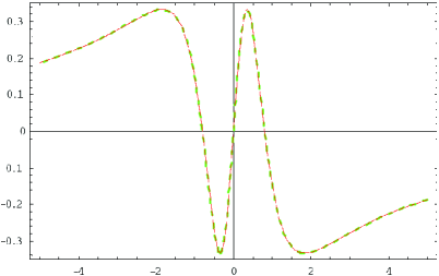
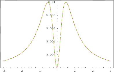
Figure 1.3: Real part (on the left) and imaginary part (on the right) of the atomic susceptibility from the full density matrix treatment as a function of the probe detuning $\delta_{p}$ (continuous line). Atomic susceptibility from equation (1.34) in unsaturated-population approximation when all population is placed in level $|{1}\rangle$ as a function of probe detuning $\delta_{p}$ (dashed line). In both cases the pump Rabi frequency was $0.8\gamma_{3}$.

We consider a density matrix which includes all relaxations channels (internal and external) and we solve it analytically in the saturated-populations form. However this analytic form is too tedious to be given here. Therefore we compare the relative solutions for the refractive index and for the extinction coefficient with the solutions of our approximated closed form. We note a perfect agreement in the EIT region, with probe detuning $\delta_{p}$ close to zero; so in this region we can analyze the refractive index, the absorption coefficient, the possibility of having amplification without inversion and the propagation of a gaussian pulse using the approximated solution to Eqs. (1.25), resolved in the unsaturated-populations form, considering negligible populations effects and all external and collisional decay rates.

This comparison is shown in Fig. 1.3 for the real and the imaginary part of the atomic susceptibility on the probe detuning $\delta_{p}$ between the exact saturated-populations solution and the unsaturated-populations approximation: the agreement is very good.

Chapter 2 Propagation in EIT media

Since the early work of Sommerfeld and Brillouin [50] on light pulse propagation, a great deal of attention has been devoted to the subject of anomalous propagation in absorbing media. In the anomalous dispersion region the group velocity $v_{g}$ may exceed the speed of light in vacuum $c$ or become even negative. Negative $v_{g}$’s require a group advance as first predicted by Garrett and McCumber [51] and then verified experimentally by Chu and Wong [52] for optical pulses propagating through layers of GaP:N. Group advances due to negative group velocities for other frequency domains have also been anticipated by Chiao and coworkers [53, 54, 55] to occur in the nearly transparent spectral region of an amplifying medium. In this chapter we will show how to obtain anomalous propagation in EIT domain but mainly we will focus on the possibility to slow light pulses, useful to realize quantum memory as will be shown in chapter 3.

Many of the important properties of EIT result from the fragile nature of quantum interference in a material that is initially opaque. Indeed the ideal transparency is attained only if the frequency difference between the two laser fields precisely matches the frequency separation between the two lower states. If matching is not perfect, the interference is not ideal and the medium becomes absorbing. Hence the transparency spike that appears in the absorption spectrum is typically very narrow. The tolerance to frequency mismatch can be increased by using stronger coupling fields, because then interference becomes more robust.

In an ideal EIT atoms are decoupled from the light fields, so the refractive index at resonance is nearly equal to unity. This means that the propagation velocity of a phase front (that is, the phase velocity) [see Sec. 2.1] is equal to that in vacuum. However, the narrow transparency resonance is accompanied by a very steep variation of the refractive index with frequency. As a result the envelope of a wavepacket propagating in the medium moves with a group velocity $v_{g}$ [47] that is much smaller than the speed of light in vacuum, $c$: so it is possible to slow light pulses. Actually $v_{g}$ depends on the control field intensity and the atomic density: decreasing the control power or increasing the atom density makes $v_{g}$ slower.

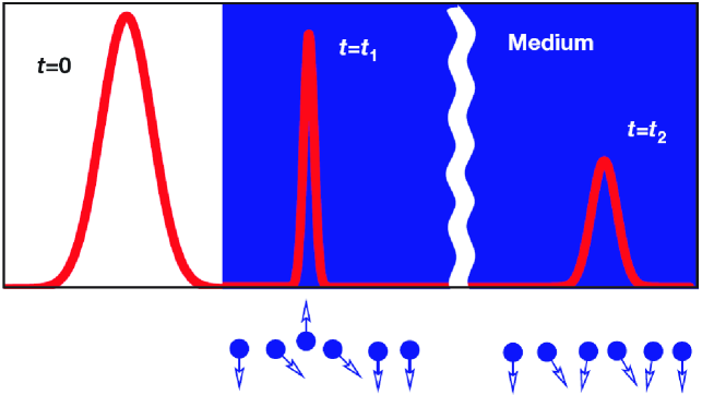
Figure 2.1: Schematic of spatial compression exhibited when a light pulse (red curve) enters the slow medium (blu). Photons are converted into flipped spins (blu arrowed circles) and the slow photonic and spin waves then propagate together. For long distance ($t_{2}\gg t_{1}$), the lossless propagation is limited by the spreading of the pulses owing to the narrow bandwidth of the transparency window. [44]

Figure 2.1 illustrates pictorially the dynamics of light retarded propagation in an EIT medium. Initially the pulse is outside the medium in which all atoms are in their ground states ($|1\rangle$). The front edge of the pulse then enters the medium and is rapidly decelerated. Because it is still outside the medium, the back edge propagates with vacuum speed c. Thus, upon entrance into the cell the spatial extent of the pulse is compressed by the ratio $\frac{c}{v_{g}}$, whereas its peak amplitude remains unchanged. Clearly the energy of the light pulse is much smaller when it is inside the medium. The rest of the photons are being expended to establish the coherence between the states $|1\rangle$ and $|2\rangle$, or in other words to flip atomic spins, with any excess energy carried away by the control field. The wave of flipped spins now propagates together with the light pulse. As the pulse exits the medium its spatial extent increases again and the atoms return to their original ground state; the pulse however, is delayed as a whole by $\Delta t=(1/v_{g}-1/c)L$ where $L$ is the length of the medium. For example, in the experiments by Hau [44] and collaborators, a pulse that is 760 m long in free space is compressed by a factor of $10^{7}$ to a length of 43 $\mu$m.

One might expect that the EIT technique could take the group velocity all the way to zero but it is not really true. Indeed to reduce the velocity more one first must make the coupling laser weaker, but reducing the coupling laser intensity also reduces the bandwidth, or frequency spread, of the incoming signal light that can be affected by. If the probe beam has a wider bandwidth, much of it will be absorbed by the atomic medium and not slowed. As the coupling intensity approaches zero - the condition for zero group velocity - the allowed bandwidth for the incoming signal beam is zero, and no light can propagate. Nevertheless we will see in the next chapter that it is possible to stop the probe field with an adiabatic control of the pump laser because in this case there is a simultaneous narrowing of transmission and pulse spectrum.

2.1 Definitions of wave velocity

In their classic treatment of the propagation of light in dispersive media, Sommerfeld and Brillouin [50] introduced five different kinds of wave velocities:

• The phase velocity, which is the speed at which the  zero crossings  of  the carrier wave move.

• The group velocity, at which the peak of a wave packet moves.

• The energy velocity, at which the energy is transported by the wave.

• The signal velocity, at which the half-maximum wave amplitude moves.

• The front velocity, at which the first appearance of a discontinuity moves.

All five velocities can differ from each other. In linear response dispersive media, the group, energy, signal, and front velocities coincide and are usually less than the phase velocity. However, recent experimental demonstrations that the group velocity of light can be reduced by 10-100 million compared with its phase velocity have fuelled many studies and exciting discussions. As noted before, these remarkable results are based on usage of very steep frequency dispersion in the vicinity of narrow resonance of electromagnetically induced transparency.

It is well known that any reactive medium leads to a delay of electromagnetic pulses and a system as simple as an infinite chain of RLC circuits can significantly reduce the speed of an electromagnetic pulse resonant within the circuit. Nevertheless from the RLC analogy it might seem that to have slow light one does not need any optical nonlinearity.

An interesting aspect of ultraslow light is that this essentially “linear” phenomenon appears in coherently driven atomic media with extremely nonlinear optical behavior where the usual optical laws concerning dispersion and absorption are no longer valid. Surprisingly, media prepared for the conditions giving raise to slow light provide new regimes of nonlinear interaction with highly increased efficiency even for very weak light fields. These media hold promise for high-precision spectroscopy and magnetometry. Besides the ability to manipulate single photon states is extremely important for the future telecommunications, as shown in this thesis.

2.2 A semi-classical approach

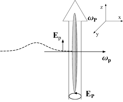
Figure 2.2: A gaussian and linearly polarized weak probe–pulse propagating along the radial $x$-axis of a cigar–shaped cloud of trapped atoms. A stronger pump–pulse right circularly polarized propagates along the longitudinal $z$-axis.

Let us calculate the effects of propagation of a gaussian pulse through a thin trapped “cloud” of atoms referring to a particular experiment on ${}^{87}Rb$ near Bose-Einstein condensation proposed in [56].

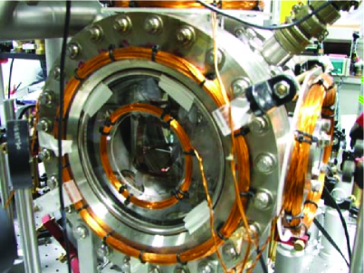
Figure 2.3: Experimental apparatus to confine ${}^{87}Rb$ atoms in a temporal dark SPOT (SPontaneous-force Optical Trap) in order to realize light propagation in cold atoms. This is a magneto-optical trap (MOT) where the repumping beam has been temporarily shut off. (Quantum Information Laboratory, Scuola Superiore di Catania)

We take the pulse to be gaussian in form and propagating across the radial width ($d=10\ \mu m$) of the cloud (see Fig. 2.2) whose optical thickness is much smaller than the incident pulse length $\cal{L}$. The medium is modelled by the square density profile of a “slab” having uniform density. In the EIT region reflection is almost vanishing [34] and the sharp boundaries of the slab of thickness $d$ don’t introduce substantial errors.

To analyze the pulse shape modifications, we assume a complex refractive index $n(\omega)$ that varies slowly over the frequency band-width $c/\cal{L}$ of the pulse so as to expand the optical wave vector around the pulse carrier frequency $\omega_{c}$,

$$k(\omega) = \frac{\omega\eta(\omega)}{c}+i\frac{\omega\kappa(\omega)}{c}\simeq k_{c}+(k^{\prime}_{cr}+ik^{\prime}_{ci})(\omega-\omega_{c})+$$ (2.1)

$$+\frac{1}{2}(k^{\prime\prime}_{cr}+ik^{\prime\prime}_{ci})(\omega-\omega_{c})^{2}$$

where $k_{c}=\omega_{c}n(\omega_{c})/c\equiv\omega_{c}(\eta_{c}+i\kappa_{c})/c$. Here $\eta(\omega)$ and $\kappa(\omega)$ denote respectively the real refractive index and the extinction coefficient while $\eta_{c}$ and $\kappa_{c}$ are their values at $\omega_{c}$. In the linear term the prime denotes the frequency derivative, which is divided into its real ($r$) and imaginary ($i$) parts, i.e. the dispersion of the real refractive index, which is related to the group velocity according to $k^{\prime}_{cr}=1/v_{g}$, and the dispersion $k^{\prime}_{ci}$ of the extinction coefficient. Moreover in the quadratic term the real part, $k^{\prime\prime}_{cr}$, characterizes the lowest order contribution to the $v_{g}$’s dispersion.

Defining $\Delta x$ the shift in the peak position relative to the position it would have in free-space, we note that for positive $v_{g}$’s which are smaller than c the peak position is retarded ($\Delta x<0$) with respect to the free–space value whereas peak position advances occur for positive $v_{g}$’s which are larger than c ($0<\Delta x<d$) or negative $v_{g}$’s ($\Delta x>d$) leading to apparent superluminal propagation.

We will derive the analytical expressions for the group velocity $v_{g}$, its dispersion $d_{g}$ and the probe transmission intensity $G_{T}$ specific to very cold alkali atomic vapors, as in the paper [56]. In Fig. 2.4 we show the level scheme for the ${}^{87}Rb$ $D_{1}$ line as concrete example of Fig. 1.1. In particular the excited state $|{3}\rangle$ can decay to the ground states $|{1}\rangle$ and $|{2}\rangle$ with rates $\Gamma_{1}$ and $\Gamma_{2}$ respectively, and the level $|{1}\rangle$ decays to levels outside those considered here with rate $\Gamma_{12}$.

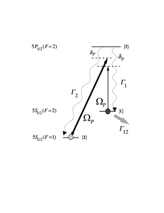
Figure 2.4: Level scheme for the ${}^{87}Rb$ $D_{1}$ line. The three levels are coupled by a pump laser with a Rabi frequency $\Omega_{P}$ and a probe field with a Rabi frequency $\Omega_{p}$. Only the hyperfine ground sub-levels $|{1}\rangle$ and $|{2}\rangle$ can be initially populated. The relevant linewidths are $\Gamma_{1}/2\pi\simeq\Gamma_{2}/2\pi\simeq\gamma_{3}/2\pi=5.75$ MHz while $\Gamma_{12}/2\pi\simeq 1$ KHz.

In Eq. (2.1) the group velocity $v_{g}$, its dispersion $d_{g}$ and the probe transmission intensity $G_{T}$ are represented by:

$$v_{g}=\frac{c}{\eta(\omega)+\omega\frac{\partial\eta(\omega)}{\partial\omega}}$$ (2.2)

$$d_{g}(\omega)=-\frac{v_{g}^{2}(\omega)}{c}\left(\omega\ \frac{\partial^{2}\eta(\omega)}{\partial\omega^{2}}+2\frac{\partial\eta(\omega)}{\partial\omega}\right)=-v_{g}^{2}(\omega)\frac{\cal{D}(\omega)}{\Gamma_{1}}$$ (2.3)

$$G_{T}(\omega)=|T(\omega)|^{2}=\Bigg{|}\frac{4n(\omega)e^{i\left[n(\omega)-1\right]\omega d/c}}{\left[n(\omega)+1\right]^{2}-\left[n(\omega)-1\right]^{2}e^{2in(\omega)\omega d/c}}\Bigg{|}^{\ 2}$$ (2.4)

where $\eta(\omega)$ is the real part of the refractive index $n(\omega)$, $d$ is the length of the atomic medium and $c$ the speed of light in vacuum. We have defined a group velocity dispersion function $\cal{D}(\omega)$ that has the dimension of a reciprocal velocity.

Now we use a density matrix treatment as in Sec. 1.5 and expand in powers of the probe Rabi frequency. For weak probe intensities the complex steady-state atomic susceptibility exhibited to the probe can be fully accounted for by the first order expansion,

$$\chi_{p} = 3\pi{\cal{N}}_{p}\Gamma_{1}\Big{[}\frac{(\delta_{p}-i\gamma_{1})}{(\delta_{p}-i\gamma_{3})(\delta_{p}-i\gamma_{1})-(\Omega_{P}/{2})^{2}}(n_{1}-n_{3})+$$ (2.5)

$${}-\frac{i}{\gamma_{3}}(\Omega_{P}/{2})^{2}\frac{(n_{3}-n_{2})}{(\delta_{p}-i\gamma_{3})(\delta_{p}-i\gamma_{1})-(\Omega_{P}/{2})^{2}}\Big{]}$$

where ${\cal{N}}_{p}$ is the scaled sample average density $(\lambda_{p}/2\pi)^{3}N/V$, $\lambda_{p}$ is the probe resonant wavelength and $n_{i}$ is the normalized population of level $i$. The overall dephasings $\gamma_{3}=(\Gamma_{1}+\Gamma_{2})/2$ and $\gamma_{1}=\Gamma_{12}/2$ of levels $|{3}\rangle$ and $|{1}\rangle$ are expressed in terms of the respective levels linewidths (see Fig. 2.4). We denote by $\delta_{p}=\omega_{31}-\omega_{p}$ the probe detuning while the pump beam is taken to be exactly at resonance ($\omega_{P}=\omega_{32}$). In equation (2.5) we also neglect contributions due to the atomic velocity distribution, since these can be eliminated by choosing a co–propagating pump and probe laser configuration.

In obtaining equation (2.5) we have assumed that the populations of the levels do not vary much with time. This assumption is justified since the Rabi frequency of the pump laser $\Omega_{P}$ is smaller than the excited state linewidth $\gamma_{3}$ ($\Omega_{P}<\gamma_{3}$) and the probe laser is taken to be much weaker than the pump. Furthermore, because the excited state $|{3}\rangle$ may decay to other atomic levels outside the two considered here, in all the following we will assume $n_{3}=0$. In order to check the validity of these assumption we have solved the full system of optical Bloch equations for an open three–level system including the possibility to pump population in any of the three levels and the possibility for the population to decay to levels outside those considered here from any of the three levels.

The dispersive behavior of the real refractive index $\eta_{p}$ fully determines the group velocity $v_{g}$ which acquires a positive minimum at resonance where the slope of $\eta_{p}$ is largest. We consider the case $n_{2}=n_{3}=0$ and $n_{1}=1$ analytically. With the help of Eq. (2.5) and a power expansion of $\eta_{p}$ around probe resonance we obtain for this minimum

$$\frac{c}{v_{g,min}^{(+)}}=1-\frac{3\pi{\cal{N}}_{p}}{2}\frac{\omega_{31}\Gamma_{1}}{\gamma_{3}^{2}}\frac{\gamma_{1}^{2}-\frac{\Omega_{P}^{2}}{4}}{\left(\gamma_{1}+\frac{\Omega_{P}^{2}}{4\gamma_{3}}\right)^{2}}$$ (2.6)

The group velocity exhibits inversion at points where the slope of $\eta_{p}$ vanishes. For small extinctions $\kappa_{p}$ this occurs approximately at the extrema of the real part of $\chi_{p}$ where, to the lowest order in $\gamma_{1}$, the probe detuning takes the value $\delta_{\infty}\simeq\pm(\gamma_{3}-\sqrt{\gamma_{3}^{2}+\Omega_{P}^{2}})/2$.

Under those experimental conditions in [56], minima of the negative group velocity occur at about twice $\delta_{\infty}$ and (in the lowest order in $\gamma_{1}$)

$$\frac{c}{v_{g,min}^{(-)}} = -\frac{3\pi{\cal{N}}_{p}}{2}\frac{\omega_{31}\Gamma_{1}}{\gamma_{3}^{2}}\left(1+\frac{\Omega_{P}^{2}}{4\ r^{2}\gamma_{3}^{2}}\right)\frac{1-r^{2}(1-\frac{\Omega_{P}^{2}}{4\ r^{2}\gamma_{3}^{2}})^{2}}{\left[1+r^{2}(1-\frac{\Omega_{P}^{2}}{4\ r^{2}\gamma_{3}^{2}})^{2}\right]^{2}}$$ (2.7)

where $r=1-\sqrt{1+(\Omega_{P}/\gamma_{3})^{2}}$ and the last factor on the right hand side of Eq. (2.7) is of the order of unity. In correspondence to these minima the group velocity dispersion in Eq. (2.3) vanishes and small group velocity deviations about $v_{g,min}^{(-)}$ are essentially determined by the dimensionless dispersion function $\cal{D}$.

Within the transparency region, for which $\eta_{p}\simeq 1$ and $\kappa_{p}\ll 1$, under these particular approximations, in terms of the detuning, Eq. (2.4) for the probe transmission intensity $G_{T}$ reduces to

$$G_{T}(\delta_{p})=e^{-2\kappa_{p}\omega_{31}d/c}\simeq e^{-\delta_{p}^{2}/2\Gamma_{G}^{2}}$$ (2.8)

The approximate expression on the right hand side holds only for appropriately small detunings ($\delta_{p}\lesssim\gamma_{3}$) since in this case $\kappa_{p}\simeq 24\pi{\cal{N}}_{p}(\gamma_{3}\Gamma_{1}\delta_{p}^{2}/\Omega_{P}^{4})$ to the lowest order in $\gamma_{1}$. The transmission bandwidth

$$\Gamma_{G}\simeq 0.06\times\frac{\Omega_{P}^{2}}{\sqrt{\gamma_{3}\Gamma_{1}}}\sqrt{\frac{c}{\omega_{31}d\ {\cal{N}}_{p}}}$$ (2.9)

increases with the pump intensity and with decreasing values of the atomic density and radial width $d$.

Let us make some remarks about the probe propagation in classical electromagnetic theory. In the presence of absorption the steady-state macroscopic atomic polarization, induced by a time-independent electric field amplitude, would simply radiate a field that cancels part of the incident field with a subsequent decrease in transmission. The situation changes for a field envelope that varies in time: during the leading half of the pulse the field amplitude rises which results into polarizations that are smaller than the steady-state value while the reverse takes place during the trailing half of the pulse. The macroscopic polarization is responsible for the absorption of energy from the probe so that the larger polarizations induced during the trailing half of the probe imply that more energy will be absorbed from the tail than from the front of the pulse. This asymmetric absorption of energy will reshape the incident gaussian pulse into a smaller, but practically undistorted, wavepacket whose peak appears to have moved faster than $c$, i.e. advanced with respect to the one that has travelled in vacuum.

Moreover, we will show that it is also possible that the peak of the pulse appears to have moved slower than $c$, i.e. retarded with respect to the one that has travelled in vacuum, when we consider zero detuning, as obtained experimentally by Hau and coworkers.

For our numerical analysis of pulse propagation across the atomic sample, we also calculate the expectation value after transmission of the probe pulse normal-order Poynting vector [57, 58], which is

$$S(x,t) = \left|\int_{0}^{\infty}d\omega_{p}\left(\frac{\hbar\omega_{p}}{2\pi S}\right)^{1/2}f(\omega_{p})T(\omega_{p})e^{i\omega_{p}(\frac{x}{c}-t)}\right|^{2}$$ (2.10)

$$\simeq \frac{S_{o}}{4\pi\sigma_{p}^{2}}\left|\int_{-\infty}^{\infty}d\delta_{p}T(\delta_{p})e^{-i\delta_{p}(\frac{x}{c}-t)}e^{-\frac{(\delta_{p}-\delta_{c})^{2}}{4\sigma_{p}^{2}}}\right|^{2}$$

where $S$ is a reference area in the $yz$-plane, $\delta_{c}=\omega_{31}-\omega_{c}$ and $S_{o}$ is the peak–power density of the incident pulse.

Here

$$f(\omega_{p})=\left(\frac{1}{2\pi\sigma_{p}^{2}}\right)^{1/4}exp\left\{{-\frac{(\omega_{p}-\omega_{c})^{2}}{4\sigma_{p}^{2}}}\right\}$$ (2.11)

denotes the frequency distribution of the incident gaussian wavepacket with carrier frequency $\omega_{c}$ and mean–square spatial length ${\cal{L}}_{p}^{2}=c^{2}/\sigma_{p}^{2}$ while $T(\omega_{p})$ is the exact transmission coefficient defined in (2.4). The transmitted average power density (2.10) is evaluated with the help of the transmission amplitude (2.4) and results are illustrated in the following sections, in which we integrate numerically this integral and we observe a reshaping and a shift of the propagated pulse, under different conditions.

2.3 Normal dispersion region

In the following figures, using the dependence of the real and imaginary parts of the optical coherence $\rho_{13}$ on the probe detuning $\delta_{p}$, we show the lineshapes of the index of refraction and of the absorption coefficient of the medium depending on $\delta_{p}$. Particularly, the gray line indicates the situation in which all population is in the level 1, the red lines show the cases in which there are the following populations:

• $n_{1}=0.9\ \ n_{2}=0.1\ \ n_{3}=0$

• $n_{1}=0.7\ \ n_{2}=0.3\ \ n_{3}=0$

• $n_{1}=0\ \ n_{2}=1\ \ n_{3}=0$ (complete inversion)

Note that for $n_{2}>n_{1}$ we have population inversion; of course, we impose the normalization of the populations, i.e. $n_{1}+n_{2}+n_{3}=1$.

Firstly, we consider the “normal” situation in which there is no pump field, no dark state and therefore there isn’t EIT.

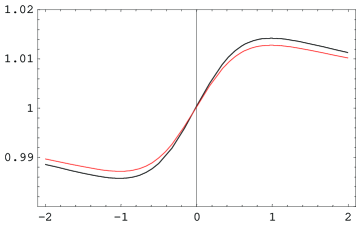
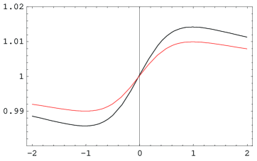
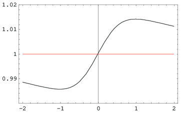
Figure 2.5: Refractive index vs detuning $\delta_{p}$ (in units of $\gamma_{3}$).

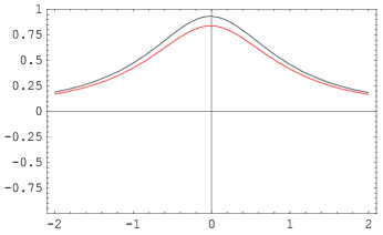
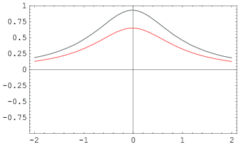
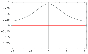
Figure 2.6: Absorption coefficient vs detuning $\delta_{p}$ (in units of $\gamma_{3}$). There is absorption, depending on $n_{1}$ (ground state), and if we take a gaussian pulse propagating across this medium with $n_{1}\neq 0$ it’s absorbed and disappears.

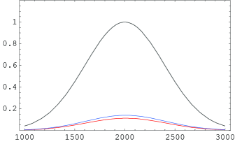
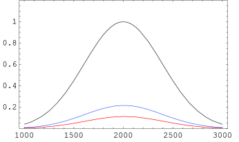
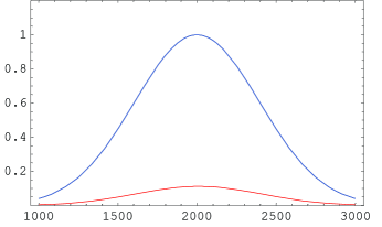
Figure 2.7: Power density $S(x,t)$ for a gaussian probe pulse in units of the incident peak power density $S_{0}(=1)$ with $x_{0}=2000$. The curves represent $S(x,t)$ as a function of x(m) after propagation in free-space (gray line) and across a cigar-shaped atomic cloud of radial width $d=10\ \mu m$ (blu lines $\rightarrow$ three different populations; red line $\rightarrow$ $n_{1}=1$). There is no coupling and the probe frequency detuning is $\delta_{p}=0$.

2.4 Anomalous dispersion region (EIT)

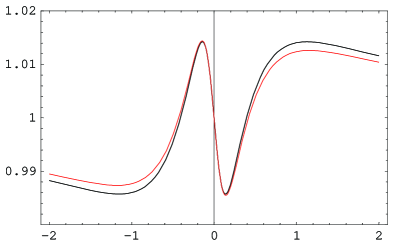
Figure 2.8: Refractive index vs detuning $\delta_{p}$ (in units of $\gamma_{3}$).

As noted before, the dependence of the real and imaginary parts of the optical coherence $\rho_{13}$ on the pump frequency $\delta_{p}$ determines the lineshapes of the index of refraction and of the absorption coefficient of the medium under coherent population-trapping resonance. We repeat the previous procedure but in the presence of coupling; in the following figures we will use the same color notation as in the previous section.

Figure 2.8 shows the lineshape of the refractive index for three fixed initial populations. We note that the central region of the detuning $\delta_{p}$ doesn’t depend on the populations, while there is this dependence for the side regions; this involves an analogous behavior for the group velocity.

In Fig. 2.9 we analyze the probe-frequency dependence of the absorption coefficient and we finally see the phenomenon of EIT with small detunings $\delta_{p}$ close to zero. Moreover we observe that with a few population ($30\ \%$) in the level 2 an amplification without inversion appears for the transition $1\leftrightarrow 3$. Indeed there is a change of sign of the absorption coefficient and with $n_{2}=0.3$ and $n_{1}=0.7$ we have a gain equal to $28\%$.

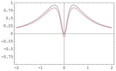
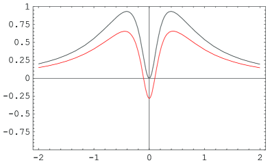
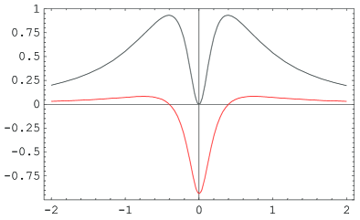
Figure 2.9: Absorption coefficient vs detuning $\delta_{p}$ (in units of $\gamma_{3}$).

We remember that $k=\omega n(\omega)/c\equiv\omega(\eta+i\kappa)/c$, where $\eta(\omega)$ and $\kappa(\omega)$ denote respectively the real refractive index and the extinction coefficient; the dispersion of the real refractive index is related to the group velocity according to $k^{\prime}_{r}=1/v_{g}$ while $k^{\prime\prime}_{cr}$ characterizes the lowest order contribution to the group velocity dispersion. Therefore we can obtain the probe-frequency dependence of the group velocity and of the relative dispersion.

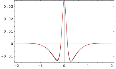
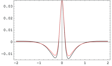
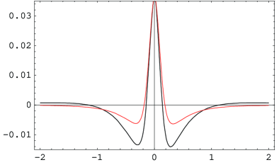
Figure 2.10: Reciprocal group velocity $(m/s)^{-1}$ vs detuning $\delta_{p}$ (in units of $\gamma_{3}$).

As noted above, the group velocity is independent of the difference of populations for detunings close to zero; in this region the group velocity is less than $c$ and then the pulse is retarded, i.e. this is the subluminal propagation. Instead, at the side regions there is a change of sign and the group velocity is negative, i.e. there is superluminal propagation, as we will note explicitly in the propagation of our gaussian pulse.

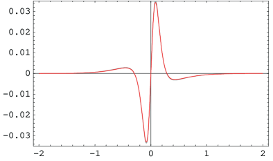
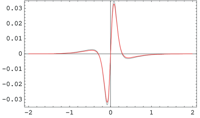
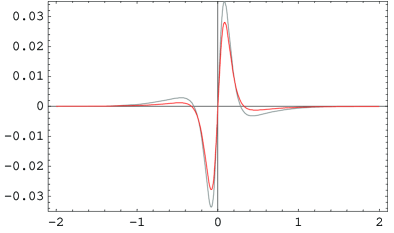
Figure 2.11: Group velocity dispersion, ${\cal D}$ $(m/s)^{-1}$, vs detuning $\delta_{p}$ (in units of $\gamma_{3}$).

Figure 2.11 shows the dispersion of group velocity. It has an important value because with zero detuning and in correspondence of minimum negative group velocity, there is no dispersion. Therefore, in these cases we analyze the propagation of a gaussian pulse in this dielectric medium.

2.5 Gain-assisted and retarded pulse

We choose the probe frequency detuning equal to zero and we observe the gain-assisted and retarded propagation of a gaussian pulse, with the usual previous values of populations.

In the following figures, the gray line represents the pulse propagating in vacuum, the red line refers to the case $n_{1}=1$, while the blue lines represent the three cases previously indicated. We note that, rising the population of the level 2, we have much more gain (we are realizing population inversion) and the group velocity is always less than $c$, i.e. retarded pulse. This behavior is in agreement with the frequency dependence of the absorption coefficient and the group velocity.

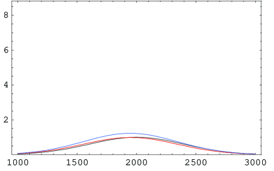
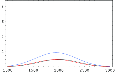
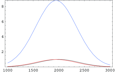
Figure 2.12: Power density $S(x,t)$ as in Fig. 2.7, but in EIT regime. The pump-beam is resonant while probe pulse has an initial frequency spread $\sigma_{p}=0.01\Gamma_{1}$ and a carrier frequency $\omega_{c}=\omega_{31}+\delta_{p}$, where $\delta_{p}=0$. The peak of the transmitted pulse has retarded by an amount $\Delta x\simeq 55m$. We note that, in second case ($n_{2}=0.3\ \ \text{and}\ \ n_{1}=0.7$), there is a peak amplification of $90\%$, while gain is $28\%$, i.e. a very slow propagation involves a very large amplification.

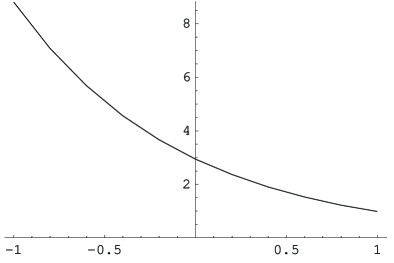
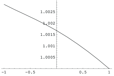
Figure 2.13: Plot of the dependence of the amplitude of the peak and of the center’s shift on the difference of the populations ($n_{1}-n_{2}$) with zero detuning. The shift’s values are normalized to that for $n_{1}=1$.

2.6 Anomalous propagation

Let us choose the probe frequency detuning corresponding to the minimum (negative) group velocity and we observe anomalous propagation. Note that the gray line represents the pulse propagating in vacuum, the red line refers to the case $n_{1}=1$, while the blue lines represent the following ones:

• $n_{1}=0.9\ \ n_{2}=0.1\ \ n_{3}=0$

• $n_{1}=0.7\ \ n_{2}=0.3\ \ n_{3}=0$

• $n_{1}=0.1\ \ n_{2}=0.9\ \ n_{3}=0$

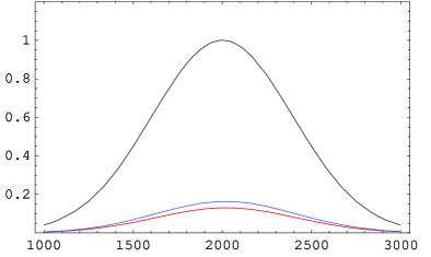
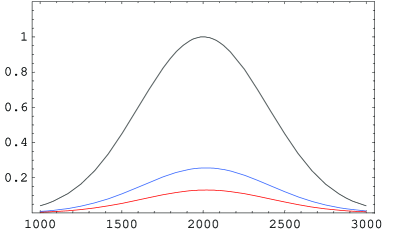
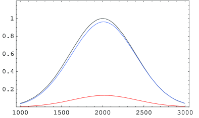
Figure 2.14: Power density $S(x,t)$ as in Fig. 2.12. The probe pulse has a carrier frequency $\omega_{c}=\omega_{31}+\delta_{min}$, where $\delta_{min}\simeq 0.28\gamma_{3}$ is the probe detuning at which $v_{g}$ reaches the smallest negative value. The peak of the transmitted pulse has advanced by an amount, respectively, $\Delta x=19.8,17.5$ and $10.6\ m$.

Now we have negative group velocity but there is absorption unless in the case of complete population inversion. In other words the propagated pulse advances one propagating in vacuum, but it is attenuated. However in the case $n_{1}=0\ \ n_{3}=0\ \ n_{2}=1$, the point of minimum negative group velocity falls inside the gain-region and it seems that we violate the principle of causality. We discuss this problem in Appendix A.2 and we note that the physics is safe.

Figure 2.16 shows that a gaussian wave packet that enters a gain medium at the entrance face at $z=0$ generates a transmitted wave packet at exit face at $z=d$ ($10\ \mu m$), whose peak leaves the exit face of the cell before the peak of the incident wave packet arrives at the entrance face.

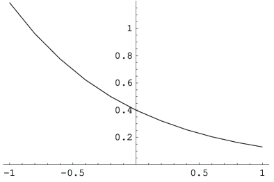
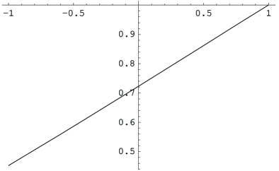
Figure 2.15: Plot of the dependence of the amplitude of the peak and of the center’s shift on the difference of the populations ($n_{1}-n_{2}$) with minimum negative group velocity. The shift’s values are normalized to the case $n_{1}=1$.

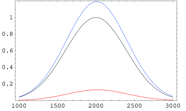
Figure 2.16: Power density $S(x,t)$ as in Fig. 2.14, with $n_{2}=1$. The peak of the transmitted pulse (blu line) has advanced by an amount $\Delta x=9.4\ m$ with a peak amplification equal to $19\%$.

2.7 A simpler system: hot atoms

Now we perform all the calculations above for a sample of a ⁸⁷Rb vapor at $35^{\circ}$C in a 10 cm long cell [59] and examine a realistic model to create the atomic population ratios needed for amplification without inversion introducing an incoherent loss rate from one of the ground levels.

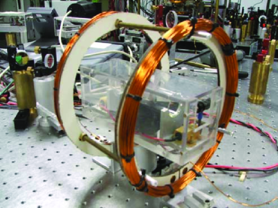
Figure 2.17: A 10 cm long cell containing ⁸⁷Rb at a temperature of $35^{\circ}$C and with density equal to $5.296\cdot 10^{7}atoms/cm^{3}$ [59]. (Quantum Information Laboratory, Scuola Superiore di Catania)

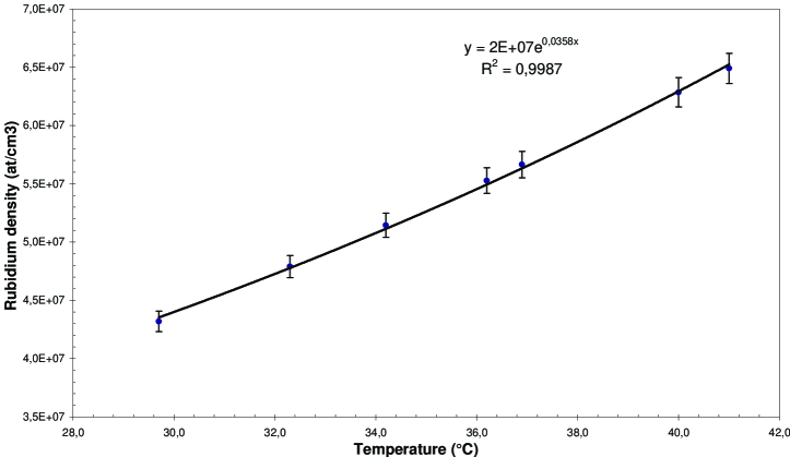
Figure 2.18: Rubidium density as function of the temperature in a 10 cm long cell containing ⁸⁷Rb.

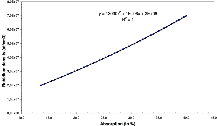
Figure 2.19: Rubidium density as function of absorption in a 10 cm long cell containing ⁸⁷Rb.

In Fig. 2.18 we report the experimental value of the Rubidium density, contained in a 10 cm long cell, at different temperatures. These results have been obtained in the Quantum Information Laboratory (Scuola Superiore di Catania) by measuring the absorption in the cell at different values of temperature. Indeed the Rubidium density is strictly connected to the absorption, as shown in Fig. 2.19.

In the same level scheme for the ⁸⁷Rb $D_{1}$ line as in Fig. 2.4 we consider the more realistic situation of a room temperature cell in which atomic populations are thermally distributed among all levels.

Therefore the initial configuration would be a nearly 50/50 distribution between the two ground states; in addition we introduce a loss mechanism from the level $|{1}\rangle$ while for level $|{3}\rangle$ we consider the correct branching ratios for ⁸⁷Rb. In Fig. 2.20 we show how the steady state population ratio between the two ground levels, even in presence of the laser beams, can indeed be varied this way while, at the same time, the amount of population placed in the excited level remains negligible. We note that a similar loss from the ground state can be easily implemented by an incoherent RF field stimulating a transition to any other ground sub–level. However this configuration has the disadvantage that while the population in level $|{2}\rangle$ increases so does the dephasing rate $\gamma_{1}$ of the ground states superposition. This strongly affects both the gain and the propagation of the pulse as discussed below.

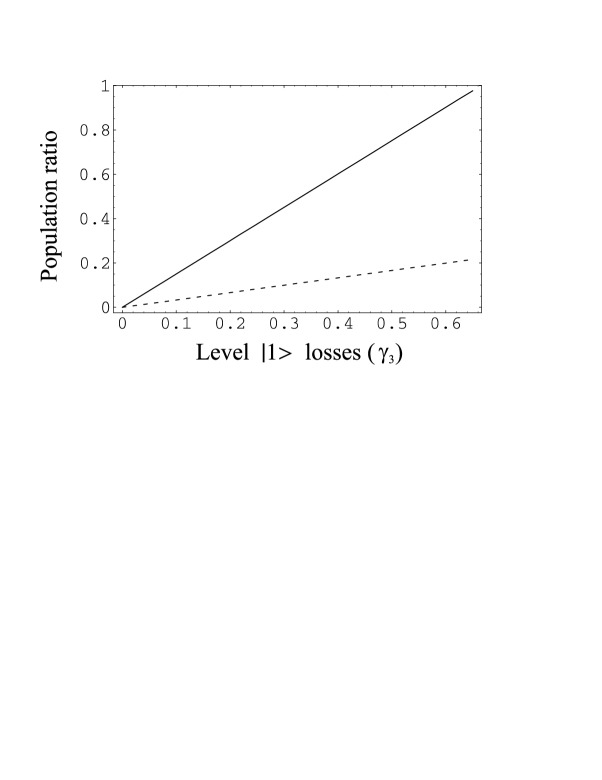
Figure 2.20: Population ratio between levels $|{2}\rangle$ and $|{1}\rangle$ (continuous line) and $|{3}\rangle$ and $|{1}\rangle$ (dashed line) as a function of the losses from level $|{1}\rangle$, $\gamma_{1}$ (in units of $\gamma_{3}$) [59].

Again we can check that the steady state atomic susceptibility computed from equation (2.5) is the same as the one computed from the full solution of the density matrix for the parameters considered here. This is shown in Fig. 2.21 left for a pump Rabi frequency of $0.8\gamma_{3}$ and $30\%$ of the atomic population in level $|{2}\rangle$. This corresponds to the situation where $\gamma_{1}=0.2\gamma_{3}$.

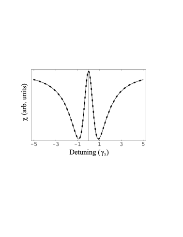
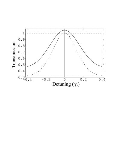
Figure 2.21: Left: Imaginary part of the atomic susceptibility from the full density matrix treatment for a loss rate from level $|{1}\rangle$ of $0.2\gamma_{3}$ as a function of the probe detuning $\delta_{p}$ (continuous line). Atomic susceptibility from equation (2.5) when $30\%$ of the population is placed in level $|{2}\rangle$ as a function of probe detuning $\delta_{p}$ (dashed line). In both cases the pump Rabi frequency was $0.8\gamma_{3}$. Right: Probe transmission as a function of probe detuning for a 10 cm long cell containing rubidium at $35^{\circ}$C, when all population is in level $|{1}\rangle$ (dashed line) and when $30\%$ of the population is in the level $|{2}\rangle$ (continuous line). In both cases the Rabi frequency of the pump laser is 0.8 $\gamma_{3}$ [59].

From equations (2.5) and (2.4) we obtain the transmission spectrum around the atomic resonance of the probe laser through a 10 cm long cell containing ⁸⁷Rb at a temperature of $35^{\circ}$C. This is reported in Fig. 2.21 right for a pump Rabi frequency of $0.8\gamma_{3}$. The transmission shows a peak in correspondence to the probe resonance, i.e. when the pump and probe lasers close a Raman transition between levels $|{1}\rangle$ and $|{2}\rangle$. This is precisely the electromagnetically induced transparency (EIT) in which the probe absorption at resonance is cancelled by destructive quantum interference between the two possible absorption paths for the probe laser, namely the two–step transition from $|{1}\rangle$ to level $|{2}\rangle$ through the excited level $|{3}\rangle$ and the Raman two–photon transition between levels $|{1}\rangle$ and $|{2}\rangle$ [48, 39]. The peak in the spectrum goes all the way to full transmission when all the atomic population is placed in level $|{1}\rangle$ (dashed line). On the contrary, when some population ($30\%$ in Fig. 2.21 right) is present in level $|{2}\rangle$ the transmission goes above unity indicating the presence of gain (continuous line). We should remark that, as shown in Fig. 2.20, no population inversion is present in the system therefore we are fulfilling the condition for gain without inversion [39]. In the situation considered here increasing the population of level $|{2}\rangle$ does not necessarily lead to extracting more gain. Indeed we are changing the population ratio by incoherently removing population from level $|{1}\rangle$, which in turn increases the dephasing rate $\gamma_{1}$ between the ground sublevels. When the dephasing increases the EIT effect is reduced and no gain is observed. In Fig. 2.22 we report the centerline gain as a function of the dephasing rate $\gamma_{1}$ with all the other experimental parameters fixed as in Fig. 2.21. As expected the gain increases to a maximum and then drops down to zero.

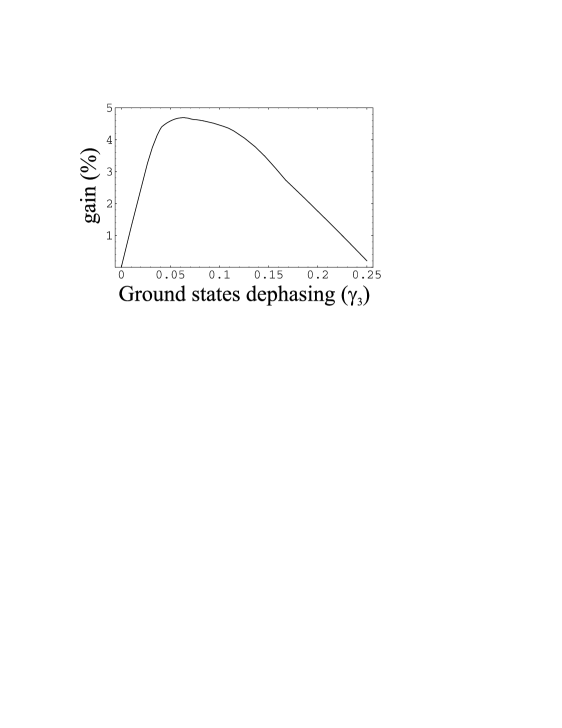
Figure 2.22: Percentage gain as function of the ground state dephasing $\gamma_{1}$ (in units of $\gamma_{3}$) for the same experimental conditions as in Fig. 2.21 [59].

Combining equations (2.2) e (2.3) with equation (2.5), we obtain the frequency dependence of the group velocity and its dispersion around the probe resonance for the same experimental parameters as before, as reported in Fig. 2.23. We note that there are three probe frequencies where the group velocity dispersion vanishes. These points correspond to frequency values where a suitable probe pulse can propagate through the medium without distortion. One of these points corresponds to the line center where we have retarded propagation. The other two, which are symmetrical with respect to the first point, correspond to anomalous propagation, i.e. a negative group velocity. We note that, when some population is placed in level $|{2}\rangle$, the positive minimum of the group velocity is increased. This is not an effect of population but of the increase in dephasing of the ground sub–levels. At the same time the negative minimum group velocity is also increased. This means that, under the conditions of gain without inversion, a propagating pulse will be slowed down while, at the same time, undergoing amplification whereas in the anomalous propagation region the pulse is advanced but not amplified, as shown for cold atoms in the previous sections. However both the pulse delay and the pulse advance are reduced with respect to normal EIT.

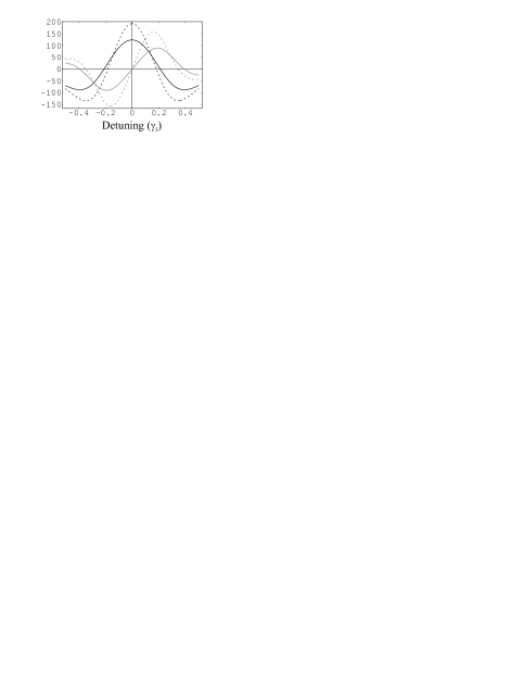
Figure 2.23: Reciprocal group velocity (black line) and group velocity dispersion function $\cal{D}$ (gray line) [(m/s)^-1] as a function of probe detuning $\delta_{p}$ (in unit of $\gamma_{3}$) for the same experimental conditions as in Fig. 2.21. Dashed lines correspond to the case when all population is in level $|{1}\rangle$, continuous lines correspond to the case when 30% of the population is in level $|{2}\rangle$. Gray curves are reduced by a factor of 10 [59].

In Fig. 2.24 we report the power density spectrum for a gaussian probe pulse propagating through a 10 cm long cell again for a pump Rabi frequency of $0.8\ \gamma_{3}$. On the left we show the resonant case where the pulse propagation is retarded. We have chosen the parameters to be at the maximum amplification (black line), in such a case the delay with respect to a pulse propagating in vacuum (grey line) is 12.2 m which amounts to a velocity of $\frac{c}{120}$ in the cell. In the normal EIT situation (dotted line) with all the population in level $|{1}\rangle$ and virtually no dephasing between the ground sublevels this delay is 18.9 m. As already mentioned, when we increase the decay rate from level $|{1}\rangle$, there is a reduction of the delay as a consequence of the larger dephasing between the ground levels. As reported in Fig. 2.25 (left) for our experimental parameters the delay is reduced below 5 m when the dephasing is equal to 0.25 $\gamma_{3}$. As reported in Fig. 2.22 at the same level of dephasing no amplification is observable.

Conversely the detuned case, shown in Fig. 2.24 right, exhibits a pulse advanced of 13.3 m with respect to the one propagating in vacuum, but the advanced propagation is accompanied by absorption. The absorption is reduced when some population is placed in level $|2\rangle$ but, at the same time, also the advance is reduced to 8.6 m. We note that the observed delay and advance can be greatly enhanced by reducing the pump Rabi frequency $\Omega_{P}$ but the effect of the levels population balance on the pulse advance is strongly suppressed. In the anomalous propagation regime, the pulse advance is decreased with respect to the normal EIT in a such way that the pulse edge never appears ahead of the edge of a pulse propagating in vacuum for the same distance. This effect is enhanced by the larger dephasing rate as shown in Fig. 2.25 (right) and the advance is below 3 m when the dephasing rate reaches 0.25 $\gamma_{3}$. We note that in the regime of population inversion the amplified pulse leading edge can indeed precede that of the vacuum propagating pulse. This is not surprising since, by inverting the atomic levels population, we are effectively storing energy in the medium [60].

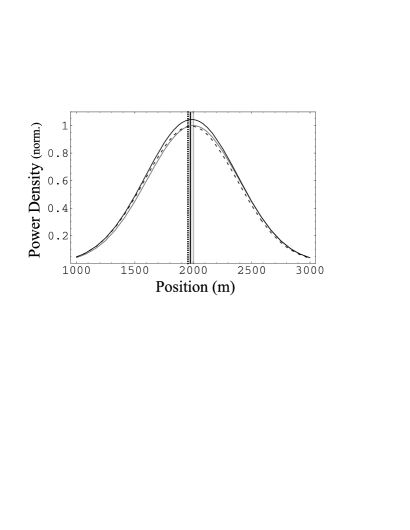
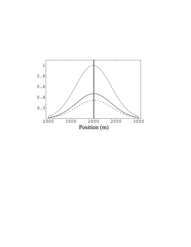
Figure 2.24: Power density for a gaussian probe pulse normalized to the pulse propagating in vacuum. On the left, the peak central frequency is on resonance resulting in retarded pulse propagation. The vertical lines in the plot indicate the center of masses of the pulses. On the right, the probe detuning corresponds to the negative minima of reciprocal group velocity showing advanced propagation. The gray line refers to the pulse propagating in vacuum, the dashed line to the case where all population is in the level $|{1}\rangle$ and the black continuous line to the case where $30\%$ of the population is in the level $|{2}\rangle$. Experimental parameters are the same as the Fig. 2.21 [59].

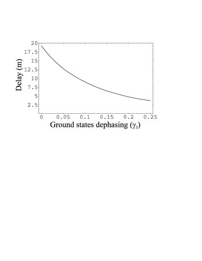
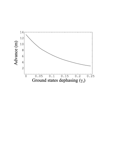
Figure 2.25: On the left pulse delay, on the right pulse advance as a function of the dephasing rate $\gamma_{1}$ (in units of $\gamma_{3}$) for the same experimental parameters as in Fig. 2.24 [59].

Finally this model is easily extendable to the case of weak coherent fields to study decoherence in quantum memories as well as to discuss amplification without inversion in connection with photon cloning. It will be object of the next chapters.

Chapter 3 Quantum memory for photons

3.1 Definition of Quantum Memory

A classical memory keeps a bit for a long time by using an huge redundancy for the two possible bit values, 0 and 1. When we consider a quantum bit or qubit this technique becomes more complicated, but still we can provide an appropriate definition of quantum memory:

• A quantum memory is a device where a quantum state can be kept for a long time and be fetched when desired with excellent fidelity.

Clearly, both “a long time” and “excellent fidelity” are determined by the desired task for which the state is kept. Indeed a quantum state develops in time according to some unitary operation and is inevitably exposed to interactions with the environment. If redundancy is added in a simple way as in the classical case, we might lose all the advantages of using quantum states. Thus, it is not easy to keep a quantum state unchanged for a long time and the same problem appears when we want to transmit a state over a long distance. However, with existing technology, one can talk about transmissions of quantum states (e.g. sending photons’ polarization states to a distance of 100 kilometers), while it does make much sense to discuss memories where a state can be kept for a few milliseconds. Let us consider a quantum bit (a two–level quantum system) in a state

$$\psi={\alpha\choose\beta}$$ (3.1)

If it changes according to some unitary transformation to a state

$$\tilde{\psi}={\tilde{\alpha}\choose\tilde{\beta}}$$ (3.2)

we may still be able to use it if we know the transformation, but if it decoheres due to interactions with other systems, in a way which we cannot reverse in time, the state is lost. As in the case of transmission over a long distance — one can choose some acceptable error rate, $P_{e}$, and agree to work with the experimental system as long as the estimated error rate $p_{e}$ does not exceed $P_{e}$. To estimate the error rate, one first does all effort to re-obtain the desired state (i.e. take the unitary transformation into consideration) and then one compares the expected state $\tilde{\psi}$ with the obtained state $\rho$ and defines the error rate as the percentage of failure. In theory, if we consider some irreversible change to the state (due to environment, or an eavesdropper, or any other reason) and we can calculate the obtained state, the error rate is

$$p_{e}=1-F(\tilde{\psi},\rho)=1-\langle\tilde{\psi}|\rho|\tilde{\psi}\rangle$$ (3.3)

where $\rho$ is the final state after the interactions and $F(\tilde{\psi},\rho)$ is the fidelity between the two states, $\tilde{\psi}$ and $\rho$ (see Appendix A.3).

The definition of quantum memory contains more that just the ability to preserve a quantum state for a long time. Other necessary conditions are the input/output abilities: one must be able to produce a known quantum state, to input an unknown state into the memory, to measure the state in some well defined basis. Moreover one needs to take it out of the memory (without measuring it) in order to perform any unitary transformation on it or alone or together with other quantum systems.

All these reasons are sufficient to understand that realizing a quantum memory is a very challenging task.

3.2 EIT in quantum information science

The propagation of the light in an EIT medium is associated with the existence of quasi-particles, which Fleischhauer [27] call dark–state polaritons (DSP). A dark–state polariton is a mixture of electromagnetic and collective atomic excitations of spin transitions (spin-wave).

Recently the authors in [23, 24, 33] have showed that it is possible to transfer adiabatically the quantum state of photons to collective atomic excitations in an EIT medium and recent experiments [26, 25] have already demonstrated the dynamic group velocity reduction and adiabatic following in the dark–state polaritons.

When a polariton propagates in an EIT medium [24], its properties can be modified simply by changing the intensity of the control beam and the polariton group velocity is proportional to the magnitude of its photonic component. As the control intensity is decreased the group velocity is slowed, which also implies that the contribution of photons in the polariton becomes purely atomic, and its group velocity is reduced to zero. At this point, quantum information originally carried by photons is mapped onto long-lived spin states of atoms. As long as the trapping process is sufficiently smooth (i.e. adiabatic), the entire procedure has no loss and is completely coherent. The stored quantum state can easily be retrieved by simply re-accelerating the stopped polariton.

In other terms, since the reduction of the group velocity happens in a linear way, the quantum state of a slowed light pulse can be preserved. Therefore a non-absorbing medium with a slow group velocity is a temporary “storage” device. However, in principle such a system has only limited “storage” capabilities; in particular the achievable ratio of storage time to pulse length can practically attain only values on the order of 10 to 100, because it depends on the square root of the medium opacity [61]. In other words this limitation originates from the fact that a small group velocity is associated with a narrow spectral acceptance window of EIT [62] and hence larger delay times require larger initial pulse length.

Figure 3.1 shows the evolution of the “signal” light pulse, spin coherence and polariton when the control beam is turned off and on. The amplitude of the signal pulse decreases as it is being decelerated whereas the spin coherence grows; the procedure is reversed when the control beam is turned back on. Besides during the adiabatic slowing the spectrum of the pulse becomes narrower in proportion to the group velocity (Fig. 3.2); so the limitations on initial spectral width or pulse length essentially disappear and very large ratios of storage time to initial pulse length can be achieved.

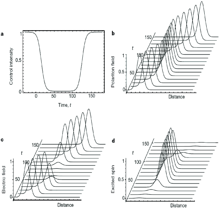
Figure 3.1: Dark–state polaritons. A dark–state polariton can be stopped and re-accelerating by ramping the control field intensity as shown in a. The coherent amplitudes of the polariton $\Psi$, the electric field $E$ and the spin components S are plotted in b to d. [27]

Figure 3.2: Simultaneous narrowing of transmission spectrum (top) and pulse spectrum (bottom) for time dependent variation of group velocity $v/c$ in units of the probe detuning $\delta_{p}$. [27]

We note here that the essential point of this technique is not to store the energy or momentum carried by photons but to store their quantum states (quantum memory). Indeed, in practice, almost no energy or momentum is actually stored in the EIT medium. Instead, both are being transferred into (or borrowed from) the control beam in such a way that an entire optical pulse is coherently converted into a low energy spin wave. After some storage time, other coupling photons are sent through the cell, the information stored in the spin excitations is transferred back to the radiation field and the original signal pulse is reconstituted. The information is transferred from purely photonic to purely atomic excitations under the control of the coupling laser. This is the key feature that distinguishes the EIT approach from earlier studies in optics or nuclear physics; it also makes possible applications in quantum information science. A different technique, to “freeze” light pulses, was suggested in [63].

Hau [44] compares the writing process to the formation of a holographic phase grating on the atomic medium; to read it out, they turn on the coupling laser and the original light pulse comes out. Marlan Scully of Texas A& M University suggests the analogy of quantum teleportation, in which an atom having a state vector at one point in space is reproduced at another point in space; in this case it would be a photon state reproduced at a later time.

Even though EIT has already made a major impact in nonlinear optical science, commercial applications have not yet emerged. One potential area is all-optical switching and signal processing in optical communication. The most serious roadblocks on this front are materials and speed issues. Good optical control requires long coherence times and for this reason the majority of experiments made use of atomic vapors that have relatively slow response. For practical communication systems, solid state devices are desirable because of their low cost and the possibility of integration with existing technologies. Photon-photon interactions enabled by EIT can fulfil the stringent requirements on precision and efficiency imposed by quantum information processing. In particular, optical materials with large nonlinearities and low loss could be indispensable for the controlled generation of entangled states and for quantum logic operations. Several avenues for using EIT in this area have already been explored.

Figure 3.3: Atom-photon quantum network. A selected atom inside the top optical cavity coherently transfers its internal qubit onto a single-photon qubit in the cavity through the application of a classical laser pulse represented by the coupling $\Omega(t)$. The coupling $g$ is between the single-photon field in the cavity and the atom. The single photon leaks out of the top cavity, only to be caught in the lower cavity by a time-reversed and synchronized classical laser pulse $\Omega(-t).$(H. J. Kimble, CalTech.)

Earlier proposals involved the use of a coherent medium to enhance photon-photon interactions in optical cavities. The key idea is that a single photon can shift the resonant frequency such that the following photon is out of resonance and is therefore reflected. The resulting “photon blockade” effect can form the basis of a quantum switch [64]. However, the requirement of a high-quality cavity is a disadvantage from a practical point of view. Subsequent work has predicted the efficient generation of entangled photons on the basis of resonant mixing of four waves. Using EIT-based phase modulation for two slowly propagating pulses, the possibility of generating macroscopic quantum states (so-called “Schroedinger’s cat” states) of light is predicted [65] but the application of this idea to quantum logic operations is complicated by the evolution of pulse envelopes in nonlinear process.

Nevertheless, a scheme for complete quantum teleportation using this technique has recently been proposed [66]. It is also possible to note that once a dark–state polariton is converted into a purely atomic excitation in a small-sized sample, logic operations can be accomplished by promoting atoms into excited states with strong atom-atom interactions. Here the ability to exchange quantum information between photons and atoms is essential for performing operations involving distant units and for the scalability of such systems. In other words it seems convenient to store and process quantum information in matter, that forms the nodes of a quantum network, and to communicate between these nodes using photons.

In the following sections we will show how to realize a quantum memory for photons and also how to obtain amplification without inversion, a typical phenomena of EIT effect. In this way we could provide a device in which is possible to register efficiently a quantum state by compensating the unavoidable losses of the transfer with the photon propagation in gain medium.

3.3 Quantum memory for a single-mode field

In order to understand the quantum state mapping transfer, first of all, as in [27], let us consider a single mode of the radiation field, i.e. a single mode optical cavity, as a quantum probe. Recall that in Sec. 1.5 we used a classical probe between a meta-stable state and the excited one, while here we quantize that field, by using a complete quantum approach.

Consider a collection of $N$ three–level atoms with two meta-stable lower states as shown in Fig. 3.4 interacting with two single-mode optical fields. The transition $|3\rangle\to|1\rangle$ of each of these atoms is coupled to a quantized radiation mode, while the transitions from $|3\rangle\to|2\rangle$ are resonantly driven by a classical control field of Rabi-frequency $\Omega_{P}$. Analogously to Sec. 1.5, the dynamics of this system is described by the interaction Hamiltonian:

$$\hat{H}=\hbar g\sum_{i=1}^{N}\hat{a}\hat{\rho}_{31}^{i}+\hbar\Omega_{P}(t){\rm e}^{-i\omega_{P}t}\sum_{i=1}^{N}\hat{\rho}_{32}^{i}+{\rm h.c.}$$ (3.4)

where $\hat{\rho}_{\mu\nu}^{i}=|\mu_{i}\rangle\langle\nu_{i}|$ is the flip operator of the $i$th atom between states $|\mu\rangle$ and $|\nu\rangle$, $\hat{a}$ is the annihilation operator for the quantum field, $\omega_{P}$ is the pump frequency and $g$ is the coupling constant between the atoms and the quantized field mode (vacuum Rabi-frequency) which for simplicity is assumed to be equal for all atoms.

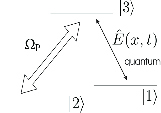
Figure 3.4: Three–level $\Lambda$-type medium resonantly coupled to a classical field with Rabi-frequency $\Omega_{P}$ and a quantum field $\hat{E}(x,t)$.

In analogy with Sec. 1.2, in this $\Lambda$–configuration, if the field is initially in a state with at most one photon, the simplest dark state is

$$|D,1\rangle = \cos\theta(t)\,|1,1\rangle-\sin\theta(t)\,|2,0\rangle$$ (3.6)

$$\tan\theta(t)=\frac{g\sqrt{N}}{\Omega(t)}$$

where $|D,1\rangle$ indicates a dark configuration with one photon.

By definition the dark states do not contain the excited state and are thus immune to spontaneous emission. In [18, 8, 23, 33] the authors show that families of dark states exist and then it is possible to transfer the quantum state of the single-mode field to collective atomic excitations. Indeed adiabatically rotating the mixing angle $\theta$ from $0$ to $\pi/2$ leads to a complete and reversible transfer of the photonic state to a collective atomic state if the total number of excitations $n$ is less than the number of atoms. This can be seen very easily in this way: If $\theta:0\to\pi/2$ one has for all $n\leq N$

$$|D,n\rangle:\,|1\rangle|n\rangle\longrightarrow|2^{n}\rangle|0\rangle$$ (3.7)

where in the final state there are $n$ atoms in the level $2$ and no photons.

Thus if the initial quantum state of the single-mode light field is in any mixed state described by a density matrix $\hat{\rho}=\sum_{n,m}\rho_{nm}\,|n\rangle\langle m|$, the transfer process generates a quantum state of collective excitations according to

$$\sum_{n,m}\rho_{nm}\,|n\rangle\langle m|\otimes|{1}\rangle\langle{1}|\longrightarrow|0\rangle\langle 0|\otimes\sum_{n,m}\rho_{nm}\,|{2}^{n}\rangle\langle{2}^{m}|$$ (3.8)

Let us point out that the quantum-state transfer does not necessarily constitute a transfer of energy from the quantum field to the atomic ensemble. Indeed in the Raman process the coherent “absorption” of a photon from the quantized mode is followed by a stimulated emission into the classical control field and then most of the energy is actually deposited in the latter field.

3.4 Propagation of a quantum field

Let us generalize to propagating fields, in three–level media under conditions of EIT, the adiabatic transfer of the quantum state from the radiation mode to collective atomic excitations, as in [27].

Consider a quantum field propagating along the radial $x$-axis of a 10 cm long cell containing rubidium at $35^{\circ}$C, as in Sec. 2.7. A quantized electromagnetic field with positive frequency part of the electric component $\hat{E}^{(+)}$ couples resonantly the transition between the ground state $|1\rangle$ and the excited state $|3\rangle$; $\omega_{p}=\omega_{31}$ is the carrier frequency of the optical field. The upper level $|3\rangle$ is furthermore coupled to the stable state $|2\rangle$ via a coherent control field with Rabi-frequency $\Omega_{P}$.

The interaction Hamiltonian reads

$$\hat{V} = -p_{31}\sum_{j}\Bigl{(}\hat{\rho}_{31}^{j}\,\hat{E}^{(+)}(x_{j})+h.c.\Bigr{)}$$ (3.9)

$$-\hbar\sum_{j}\Bigl{(}\hat{\rho}_{32}^{j}\,\Omega_{P}(x_{j},t)\,{\rm e}^{i(k^{\parallel}x_{j}-\omega_{P}t)}+h.c.\Bigr{)}$$

where $x_{j}$ denotes the position of the $j$th atom, $p_{31}$ denotes the dipole matrix element between the states $|3\rangle$ and $|1\rangle$, $\hat{\rho}_{\alpha\beta}^{j}\equiv|\alpha_{j}\rangle\langle\beta_{j}|$ defines the atomic flip operators and $k^{\parallel}=\vec{k}\cdot\vec{\rm e}_{x}=\frac{\omega_{P}}{c}\cos\vartheta$ is the projection of the wavevector of the control field to the propagation axis of the quantum field. Particularly we assume that the carrier frequencies $\omega_{p}$ and $\omega_{P}$ of the quantum and control fields coincide with the atomic resonances $\omega_{31}$ and $\omega_{32}$ respectively, i.e. we are on the EIT resonance.

Then we introduce slowly-varying variables according to

$$\hat{E}^{(+)}(x,t) = \sqrt{\frac{\hbar\omega_{p}}{2\varepsilon_{0}V}}\hat{\cal E}(x,t)\,{\rm e}^{i\frac{\omega_{p}}{c}(x-ct)}$$ (3.10)

$$\hat{\rho}_{\mu\nu}^{j}(t) = {\widetilde{\rho}}_{\mu\nu}^{j}(t)\,{\rm e}^{-i\frac{\omega_{\mu\nu}}{c}(x-ct)}$$ (3.11)

where $\varepsilon_{0}$ is the vacuum electric permittivity and $V$ is some quantization volume, which for simplicity was chosen to be equal to the interaction volume.

If the (slowly-varying) quantum amplitude does not change in a length interval $\Delta x$ which contains $N_{x}\gg 1$ atoms, we can introduce continuum atomic variables

$${\widetilde{\rho}}_{\mu\nu}(x,t)=\frac{1}{N_{x}}\sum_{x_{j}\in N_{x}}\,{\widetilde{\rho}}_{\mu\nu}^{j}(t)$$ (3.12)

and make the replacement $\sum_{j=1}^{N}\longrightarrow\frac{N}{L}\int{\rm d}x$, where $N$ is the number of atoms, and $L$ the length of the interaction volume in propagation direction of the quantized field. This yields the continuous form of the interaction Hamiltonian

$${\hat{V}}=-\int\!\!\frac{{\rm d}x}{L}\biggl{(}\hbar gN{\widetilde{\rho}}_{31}(x,t)\,\hat{\cal E}(x,t)+\hbar\Omega_{P}(x,t){\rm e}^{i\Delta kx}N(z){\widetilde{\rho}}_{32}(x,t)+h.c.\biggr{)}$$

(3.13)

where $g=p_{31}\sqrt{\frac{\omega_{p}}{2\hbar\epsilon_{0}V}}$ is the atom-field coupling constant and $\Delta k=k^{\parallel}-k=\frac{\omega_{32}}{c}\left(\cos\vartheta-1\right)$.

Therefore, in slowly varying amplitude approximation, the evolution of the Heisenberg operator corresponding to the quantum field can be described by the propagation equation

$$\left(\frac{\partial}{\partial t}+c\frac{\partial}{\partial x}\right)\hat{\cal E}(x,t)={i}gN{\widetilde{\rho}}_{13}(x,t)$$ (3.14)

On the other hand, the atomic evolution is governed by a set of Heisenberg-Langevin equations

$$\dot{{\widetilde{\rho}}}_{33} = -2\gamma_{3}{{\widetilde{\rho}}}_{33}-ig\Bigl{(}\hat{\cal E}^{\dagger}{{\widetilde{\rho}}}_{13}-h.c.\Bigr{)}-i\Bigl{(}\Omega_{P}^{*}{\rm e}^{-i\Delta kx}{{\widetilde{\rho}}}_{23}-h.c.\Bigr{)}+F_{3}$$

$$\dot{{\widetilde{\rho}}}_{11} = \Gamma_{1}{{\widetilde{\rho}}}_{33}-\Gamma_{12}\rho_{11}+ig\Bigl{(}\hat{\cal E}^{\dagger}{{\widetilde{\rho}}}_{13}-h.c.\Bigr{)}+F_{1}$$

$$\dot{{\widetilde{\rho}}}_{22} = \Gamma_{2}{{\widetilde{\rho}}}_{33}+\Gamma_{12}\rho_{11}+i\Bigl{(}\Omega_{P}^{*}{\rm e}^{-i\Delta kx}{{\widetilde{\rho}}}_{23}-h.c.\Bigr{)}+F_{2}$$ (3.15)

$$\dot{{\widetilde{\rho}}}_{13} = -(\gamma_{1}+\gamma_{3}){{\widetilde{\rho}}}_{13}+ig\hat{\cal E}\Bigl{(}{{\widetilde{\rho}}}_{11}-{{\widetilde{\rho}}}_{33}\Bigr{)}+i\Omega_{P}{\rm e}^{i\Delta kx}{{\widetilde{\rho}}}_{12}+F_{13}$$

$$\dot{{\widetilde{\rho}}}_{23} = -\gamma_{3}{{\widetilde{\rho}}}_{23}+i\Omega_{P}{\rm e}^{i\Delta kx}\Bigl{(}{{\widetilde{\rho}}}_{22}-{{\widetilde{\rho}}}_{33}\Bigr{)}+ig\hat{\cal E}{{\widetilde{\rho}}}_{21}+F_{23}$$

$$\dot{{\widetilde{\rho}}}_{12} = -\gamma_{1}{{\widetilde{\rho}}}_{12}+i\Omega_{P}^{*}{\rm e}^{-i\Delta kx}{{\widetilde{\rho}}}_{13}-ig\hat{\cal E}{{\widetilde{\rho}}}_{32}$$

where, as in Fig. 2.4, $\gamma_{3}=\frac{\Gamma_{1}+\Gamma_{2}}{2}$ and $\gamma_{1}=\frac{\Gamma_{12}}{2}$ are the overall dephasing, $\Gamma_{1}$ and $\Gamma_{2}$ are the respective levels linewidths and $F_{\mu}$ and $F_{\mu\nu}$ are $\delta$-correlated Langevin noise operators.

Using the configuration of fixed population as in Sec. 2.7 for weak quantum fields, we can assume

$${\widetilde{\rho}}_{11} = 1-\eta$$ (3.16)

$${\widetilde{\rho}}_{22} = \eta$$ (3.17)

$${\widetilde{\rho}}_{33} \simeq 0$$ (3.18)

where $\eta$ is fixed by a incoherent RF field stimulating a transition between the ground sub-levels. By using the steady-state solution to the rate equations, we find that $\eta\simeq 4\frac{\gamma_{1}}{\Omega_{P}}$ for $\eta\ll 1$.

Therefore one has for the coherence terms of the density operator:

$$\dot{{\widetilde{\rho}}}_{13} = -(\gamma_{1}+\gamma_{3}){{\widetilde{\rho}}}_{13}+ig\hat{\cal E}(1-\eta)+i\Omega_{P}{\rm e}^{i\Delta kx}{{\widetilde{\rho}}}_{12}+F_{13}$$

$$\dot{{\widetilde{\rho}}}_{23} = -\gamma_{3}{{\widetilde{\rho}}}_{23}+i\Omega_{P}{\rm e}^{i\Delta kx}\eta+ig\hat{\cal E}{{\widetilde{\rho}}}_{13}+F_{23}$$ (3.19)

$$\dot{{\widetilde{\rho}}}_{12} = -\gamma_{1}{{\widetilde{\rho}}}_{12}+i\Omega_{P}^{*}{\rm e}^{-i\Delta kx}{{\widetilde{\rho}}}_{13}-ig\hat{\cal E}{{\widetilde{\rho}}}_{32}$$

3.4.1 Low-intensity approximation

In order to solve the propagation problem, we now assume that the Rabi-frequency of the quantum field, $\Omega_{p}$, is much smaller than $\Omega_{P}$ and that the number density of photons in the input pulse is much less than the number density of atoms. In such a case the atomic equations can be treated perturbatively in $\hat{\cal E}$. By using Eqs. (3.19) and neglecting the first order terms in $\hat{\cal E}$, for $\gamma_{1}$ fixed, one obtains

$${\widetilde{\rho}}_{13}=-\frac{i}{\Omega_{P}^{*}}{\rm e}^{i\Delta kx}\big{[}\frac{\partial}{\partial t}{\widetilde{\rho}}_{12}+\gamma_{1}{\widetilde{\rho}}_{12}\Big{]}-i\frac{g}{\gamma_{3}}\eta\hat{\cal E}$$ (3.20)

Then the interaction of the probe pulse with the medium can be described by the amplitude of the probe electric field $\hat{\cal E}$ and the collective ground-state spin variable ${\widetilde{\rho}}_{12}$:

$$\left(\frac{\partial}{\partial t}+c\frac{\partial}{\partial x}\right)\hat{\cal E}(x,t)=gN\Big{\{}\frac{{\rm e}^{i\Delta kx}}{\Omega_{P}^{*}}\big{[}\frac{\partial}{\partial t}{\widetilde{\rho}}_{12}+\gamma_{1}{\widetilde{\rho}}_{12}\Big{]}+\frac{g}{\gamma_{3}}\eta\hat{\cal E}(x,t)\Big{\}}\ \ \$$ (3.21)

and

$${\widetilde{\rho}}_{12}= - \frac{g\hat{\cal E}}{B}{\rm e}^{-i\Delta kx}(1-\eta)-\frac{\gamma_{1}}{B\Omega_{P}^{*}}\frac{\partial}{\partial t}{\widetilde{\rho}}_{12}+$$

$$- \frac{i}{B}\left[\left(\frac{\partial}{\partial t}+(\gamma_{1}+\gamma_{3})\right)\left(-\frac{i}{\Omega_{P}^{*}}\frac{\partial}{\partial t}{\widetilde{\rho}}_{12}-i\frac{g}{\gamma_{3}}{\rm e}^{-i\Delta kx}\eta\hat{\cal E}\right)+{\rm e}^{-i\Delta kx}F_{13}\right]$$

where

$$B=\frac{\Omega^{2}+(\gamma_{1}+\gamma_{3})\gamma_{1}}{\Omega^{*}}.$$

3.4.2 Adiabatic limit

The propagation equations simplify considerably if we assume a sufficiently slow change of $\Omega_{P}$, i.e. adiabatic conditions [67, 61, 65].

Normalizing the time to a characteristic scale $T$ via $\tilde{t}=t/T$ and expanding the r.h.s. of (3.4.1) in powers of $1/T$ we find in lowest non-vanishing order

$${\widetilde{\rho}}_{12}(x,t)\simeq-g\frac{\hat{\cal E}(x,t)}{B}{\rm e}^{-i\Delta kx}$$ (3.22)

where we use also that $\gamma_{3}\simeq\gamma_{3}+\gamma_{1}$, because $\gamma_{1}\ll\gamma_{3}$.

We note that also the noise operator $F_{ba}$ gives no contribution in the adiabatic limit, since $\langle F_{x}(t)F_{y}(t^{\prime})\rangle\sim\delta(t-t^{\prime})=\delta(\tilde{t}-\tilde{t}^{\prime})/T$. Thus in the perturbative and adiabatic limit the propagation of the quantum light pulse is governed by the following equation

$$\left(\frac{\partial}{\partial t}+c\frac{\partial}{\partial x}\right)\hat{\cal E}(x,t) = -\frac{g^{2}N}{\Omega^{*}}\frac{\partial}{\partial t}\frac{\hat{\cal E}(x,t)}{B}+g^{2}N\Big{(}\frac{\eta}{\gamma_{3}}-\frac{\gamma_{1}}{\Omega^{*}B}\Big{)}\hat{\cal E}(x,t)$$

If $\Omega(x,t)=\Omega(x)$ is constant in time and the incoherent RF field frequency is constant, the term on the r.h.s. of the propagation equation (3.4.2) leads to a modification of the group velocity of the quantum field according to

$$v_{g}=v_{g}(x)=\frac{c}{1+n_{g}(x)}\ \ \ \ \ \ \ \ \ n_{g}(x)=\frac{g^{2}N}{\Omega_{P}^{*}B}=\frac{3}{8\pi^{2}}\frac{N}{V}\lambda_{13}^{3}\frac{kc\,\gamma}{\Omega_{P}^{*}B}$$ (3.24)

where $\frac{N}{V}$ is the atom density, $n_{g}$ is the group velocity index and $\lambda_{13}$ the resonant wavelength of the $3\to 1$ transition. In the next section we will analyze the propagation under time-dependent conditions.

3.5 Quasi-particle picture

Up to now we have considered the propagation of a quantum field in an EIT medium under stationary conditions, i.e. with a constant or only spatially varying control field. In these conditions, a coherent process that allows for an uni-directional transfer of the quantum state of a photon wavepacket to the atomic ensemble isn’t possible because the hamiltonian of the system is time-independent.

Now let us show how to realize this transfer by using a time-dependent control field. Indeed, for a spatially homogeneous but time-dependent control field, $\Omega_{P}=\Omega_{P}(t)$, the propagation problem can be solved in a very instructive way in a quasi-particle picture. As a consequence the population of the level 2 will vary in time also for effect of $\Omega_{P}(t)$, i.e. $\eta(t)\simeq 4\frac{\gamma_{1}}{\Omega_{P}(t)}$, when $\gamma_{1}$ is fixed.

Therefore we will introduce these quasi-particles, called dark–state polaritons by the authors in [24, 68], and we will show how it is possible to transfer the quantum state from the light to the matter.

3.5.1 Definition of dark- and bright-state polaritons

Let us consider the case of a time-dependent, spatially homogeneous and real control field $\Omega_{P}=\Omega_{P}(t)=\Omega_{P}(t)^{*}$.

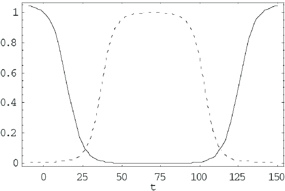
Figure 3.5: Control field (continuous line) $\Omega_{P}(t)/\Omega_{P}(0)$ as function of time according to $\Omega_{P}(t)=0.8(1-0.5\tanh[0.1(t-15)]+0.5\tanh[0.1(t-125)])$ (in units of $\gamma_{3}$). The mixed angle $\frac{\theta(t)}{\pi/2}$ (dashed line) is also reported. Parameters are $g^{2}N=1/100$.

The physically relevant variables are the electric field $\hat{\cal E}$ and the atomic spin coherence ${\widetilde{\rho}}_{12}$, so defining a rotation in the space of these variables, we can introduce two new quantum fields, $\hat{\Psi}(x,t)$ and $\hat{\Phi}(x,t)$

$$\hat{\Psi}(x,t) = \cos\theta(t)\,\hat{\cal E}(x,t)-\sin\theta(t)\,\sqrt{N}\,{\widetilde{\rho}}_{12}(x,t)\,{\rm e}^{i\Delta kx}$$ (3.25)

$$\hat{\Phi}(x,t) = \sin\theta(t)\,\hat{\cal E}(x,t)+\cos\theta(t)\,\sqrt{N}\,{\widetilde{\rho}}_{12}(x,t)\,{\rm e}^{i\Delta kx}$$ (3.26)

where the mixing angle $\theta(t)$ is such as

$$\tan^{2}\theta(t)=\frac{g^{2}N}{\Omega_{P}^{2}(t)}=n_{\rm g}(t)$$ (3.27)

Le us to point out that $\hat{\Psi}$ and $\hat{\Phi}$ are superpositions of electromagnetic ($\hat{\cal E}$) and collective atomic components ($\sqrt{N}{\widetilde{\rho}}_{12}$), whose admixture can be controlled through $\theta(t)$ by changing the strength of the external driving field.

Introducing a plain-wave decomposition $\hat{\Psi}(x,t)=\sum_{k}\hat{\Psi}_{k}(t)\,{\rm e}^{ikx}$ and $\hat{\Phi}(x,t)=\sum_{k}\hat{\Phi}_{k}(t)\,{\rm e}^{ikx}$ respectively, one finds that the mode operators obey the commutation relations

$$\Bigl{[}\hat{\Psi}_{k},\hat{\Psi}_{k^{\prime}}^{\dagger}\Bigr{]} = \delta_{k,k^{\prime}}\,\Bigl{[}\cos^{2}\theta+\sin^{2}\theta\frac{1}{N}\sum_{j}({\hat{\rho}}_{11}^{j}-{\hat{\rho}}_{22}^{j})\Bigr{]}$$ (3.28)

$$\Bigl{[}\hat{\Phi}_{k},\hat{\Phi}_{k^{\prime}}^{\dagger}\Bigr{]} = \delta_{k,k^{\prime}}\,\Bigl{[}\sin^{2}\theta+\cos^{2}\theta\frac{1}{N}\sum_{j}({\hat{\rho}}_{11}^{j}-{\hat{\rho}}_{22}^{j})\Bigr{]}$$ (3.29)

$$\Bigl{[}\hat{\Psi}_{k},\hat{\Phi}_{k^{\prime}}^{\dagger}\Bigr{]} = \delta_{k,k^{\prime}}\sin\theta\cos\theta\,\Bigl{[}1-\frac{1}{N}\sum_{j}({\hat{\rho}}_{11}^{j}-{\hat{\rho}}_{22}^{j})\Bigr{]}$$ (3.30)

In our case, ${\hat{\rho}}_{11}^{j}=1-\eta,{\hat{\rho}}_{22}^{j}=\eta$, the new fields possess the following commutation relations

$$\Bigl{[}\hat{\Psi}_{k},\hat{\Psi}_{k^{\prime}}^{\dagger}\Bigr{]} = \delta_{k,k^{\prime}}(1-2\eta\sin^{2}\theta)$$

$$\Bigl{[}\hat{\Phi}_{k},\hat{\Phi}_{k^{\prime}}^{\dagger}\Bigr{]} = \delta_{k,k^{\prime}}(1-2\eta\cos^{2}\theta)$$ (3.31)

$$\Bigl{[}\hat{\Psi}_{k},\hat{\Phi}_{k^{\prime}}^{\dagger}\Bigr{]} = 2\eta\delta_{k,k^{\prime}}\sin\theta\cos\theta\$$

Now we analyze the following two case: 1) $\eta=0$ ($\gamma_{1}=0$), 2) $\eta>0$ ($\gamma_{1}>0$).

• $\eta=0$ ($\gamma_{1}=0$)

  In this case [27] the quasi-particles satisfy bosonic commutation relations and therefore one immediately verifies that all number states created by $\hat{\Psi}_{k}^{\dagger}$,

  $$|n_{k}\rangle=\frac{1}{\sqrt{n!}}\Bigl{(}\hat{\Psi}_{k}^{\dagger}\Bigr{)}^{n}|0\rangle|1_{1}...1_{N}\rangle$$ (3.32)

  where $|0\rangle$ denotes the field vacuum, are dark–states [39, 23]. The states $|n_{k}\rangle$ do not contain the excited atomic state and are thus immune to spontaneous emission. Moreover, they are eigenstates of the interaction Hamiltonian with eigenvalue zero,

  $${\hat{V}}\,|n_{k}\rangle=0$$ (3.33)

  For these reasons the authors in [27] call these quasi-particles $\hat{\Psi}$ “dark–state polaritons”. Similarly one finds that the elementary excitations of $\hat{\Phi}$ correspond to the bright-states in three–level systems. Consequently these quasi-particles are called “bright-state polaritons”.

  Besides one can transform the equations of motion for the electric field and the atomic variables into the new field variables.

  First of all we write down $\hat{\cal E}$ and ${\widetilde{\rho}}_{12}$ in terms of the fields $\hat{\Phi}$ and $\hat{\Psi}$:

  $$\hat{\cal E} = \cos\theta\hat{\Psi}+\sin\theta\hat{\Phi}$$

  $${\widetilde{\rho}}_{12} = \frac{1}{\sqrt{N}}{\rm e}^{-i\Delta kx}(\cos\theta\hat{\Phi}-\sin\theta\hat{\Psi})$$ (3.34)

  By substituting these expressions in Eq. (3.4.2) with $\eta=0$ ($\gamma_{1}=0$), one finds

  $$\biggl{[}\frac{\partial}{\partial t}+c\cos^{2}\theta\frac{\partial}{\partial x}\biggr{]}\,\hat{\Psi}=-\dot{\theta}\,\hat{\Phi}-c\sin\theta\cos\theta\,\frac{\partial}{\partial x}\hat{\Phi}$$ (3.35)

  $$\hat{\Phi} = \frac{\sin\theta}{g^{2}N}\biggl{(}\frac{\partial}{\partial t}+\gamma_{3}\Bigr{)}\Bigl{(}\tan\theta\frac{\partial}{\partial t}\biggr{)}\Bigl{(}\sin\theta\,\hat{\Psi}-\cos\theta\,\hat{\Phi}\Bigr{)}-i\frac{\sin\theta}{g}F_{13}$$

  where one has to keep in mind that the mixing angle $\theta$ is a function of time.

• $\eta>0$ ($\gamma_{1}>0$)

  In this case the quasi–particles don’t satisfy bosonic commutation relations and the previous discussion about dark states is not possible. However, in chapter 4 from the statistical point of view we will examine this configuration because these generalized commutation relations play an important role in parastatistics.

  By using Eqs. (3.34) and by substituting these expressions in Eq. (3.4.2), we have

$$\biggl{[}\frac{\partial}{\partial t} + c\cos^{2}\theta\frac{\partial}{\partial x}-\frac{g^{2}N}{\gamma_{3}}\eta\cos^{2}\theta+\gamma_{1}\sin^{2}\theta\biggr{]}\,\hat{\Psi}=$$

$$= -\dot{\theta}\,\hat{\Phi}-c\sin\theta\cos\theta\,\frac{\partial}{\partial x}\hat{\Phi}+(\gamma_{1}+\frac{g^{2}N}{\gamma_{3}}\eta)\sin\theta\cos\theta\,\hat{\Phi}$$

$$\hat{\Phi} = \frac{1}{\cos^{2}\theta+\frac{\Omega_{P}}{B}\sin^{2}\theta}\Big{\{}(1-\frac{\Omega_{P}}{B})\sin\theta\cos\theta\hat{\Psi}+$$

$$- \frac{\gamma_{1}}{B\Omega_{P}^{*}}\cos\theta\frac{\partial}{\partial t}(\cos\theta\hat{\Phi}-\sin\theta\hat{\Psi})-\sin\theta\frac{\Omega_{P}}{B}\frac{\eta}{\gamma_{3}}\frac{\partial}{\partial t}(\cos\theta\hat{\Psi}+\sin\theta\hat{\Phi})+$$

$$+ \frac{\sin\theta}{g^{2}N}\biggl{(}\frac{\partial}{\partial t}+(\gamma_{1}+\gamma_{3})\Bigr{)}\Bigl{(}\tan\theta\frac{\partial}{\partial t}\biggr{)}\Bigl{(}\sin\theta\,\hat{\Psi}-\cos\theta\,\hat{\Phi}\Bigr{)}-i\frac{\sin\theta}{g}F_{13}\Big{\}}$$

3.5.2 Adiabatic limit

Introducing the adiabaticity parameter $\varepsilon\equiv\Bigl{(}g\sqrt{N}T\Bigr{)}^{-1}$ with $T$ being a characteristic time, one can expand the equations of motion in powers of $\varepsilon$. In lowest order, i.e. in the adiabatic limit, one finds

$$\hat{\Phi} \approx 0.$$ (3.38)

Consequently

$$\hat{\cal E}(x,t) = \enspace\cos\theta(t)\,\hat{\Psi}(x,t),$$ (3.39)

$$\sqrt{N}{\widetilde{\rho}}_{12} = -\sin\theta(t)\,\hat{\Psi}(x,t)\,{\rm e}^{-i\Delta kx}$$ (3.40)

Now let us consider the two cases, $\eta=0$ and $\eta>0$.

• $\eta=0$ ($\gamma_{1}=0$)

  In this case Eq. (3.35), in the adiabatic limit, reduces to the following very simple equation of motion of $\Psi$:

  $$\left[\frac{\partial}{\partial t}+c\cos^{2}\theta(t)\frac{\partial}{\partial x}\right]\hat{\Psi}(x,t)=0$$ (3.41)

  Eq.(3.41) describes a shape- and quantum-state preserving propagation with instantaneous velocity $v=v_{g}(t)=c\cos^{2}\theta(t)$:

  $$\hat{\Psi}(x,t)=\hat{\Psi}\biggl{(}x-c\int^{t}_{0}\!\!\!{\rm d}\tau\cos^{2}\theta(\tau),0\biggr{)}$$ (3.42)

  For $\theta\to 0$, i.e. for a strong external drive field $\Omega^{2}\gg g^{2}N$, the polariton has purely photonic character $\hat{\Psi}=\hat{\cal E}$ and the propagation velocity is that of the vacuum speed of light. In the opposite limit of a weak drive field $\Omega^{2}\ll g^{2}N$ such that $\theta\to\pi/2$, the polariton becomes spin-wave like $\hat{\Psi}=-\sqrt{N}{\widetilde{\rho}}_{12}{\rm e}^{i\Delta kx}$ and its propagation velocity approaches zero.

  This is the essence of the transfer technique of quantum states from photon wave-packets propagating at the speed of light to stationary atomic excitations (stationary spin waves). Adiabatically rotating the mixing angle from $\theta=0$ to $\theta=\pi/2$ decelerates the polariton to a full stop, changing its character from purely electromagnetic to purely atomic. Due to the linearity of Eq. (3.41) and the conservation of the spatial shape, the quantum state of the polariton is not changed during this process.

  Likewise the polariton can be re-accelerated to the vacuum speed of light; in this process the stored quantum state is transferred back to the field. This is illustrated in Fig. 3.6, where the coherent amplitude of the pulse field is showed during the storing and the following releasing.

• $\eta>0$ ($\gamma_{1}>0$)

  When there is population ($\eta$) in the level 2, $\hat{\Psi}$ obeys the following equation of motion

  $$\biggl{[}\frac{\partial}{\partial t} + c\cos^{2}\theta\frac{\partial}{\partial x}-\frac{g^{2}N}{\gamma_{3}}\eta\cos^{2}\theta+\sin^{2}\theta\gamma_{1}\biggr{]}\,\hat{\Psi}=0$$ (3.43)

  By varying the dephasing ($\gamma_{1}$) between the two lower-states, there is a balance between two $\gamma_{1}$-induced effects: the destruction of the EIT window at higher dephasings and the amplification without inversion produced by the population in the level 2. The situation is represented in Fig. 3.7 for different values of $\gamma_{1}$. In one case in Fig. 3.7, we have an amplification of dark–state polariton, that at least compensates the unavoidable losses in the process of storing and releasing.

  One could speculate that in this way it could be possible to obtain also a quantum cloning (continuous-variable) of a coherent state into the quantum memory described above. However this needs to be verified and it will not be treated in this thesis.

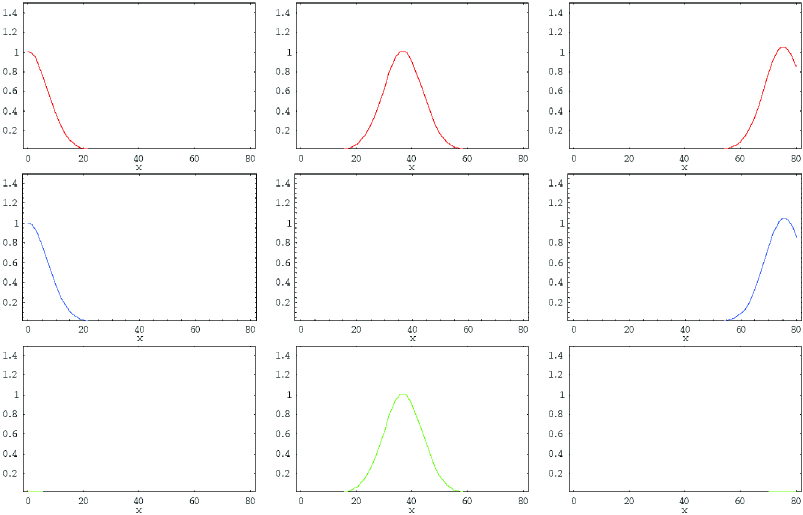
Figure 3.6: Propagation of a dark–state polariton with envelope $\exp\{-(x/10)^{2}\}$ for three time slices corresponding to $\theta(t)=0,\ \pi/2,\ 0$, in the case $\eta=0$ ($\gamma_{1}=0$), i.e. ideal EIT regime. The mixing angle is rotated from $0$ to $\pi/2$ and back according to $\cot\theta(t)=0.8(1-0.5\tanh[0.1(t-15)]+0.5\tanh[0.1(t-125)])$. The coherent amplitude of the polariton $\Psi=<\hat{\Psi}>$ (red line), the electric field $E=<\hat{E}>$ (blu line) and the matter components $|\rho_{12}|=|<\hat{\rho}_{12}>|$ (green line) are plotted. Through the dynamic rotation of the mixing angle, it is possible to obtain an adiabatic passage from a pure photon-like to a pure spin-wave polariton, i.e. decelerating the initial photon wavepacket to a full stop. Therefore the quantum state of the optical field is completely transferred to the atoms. Afterwards the photon wave-packet is regenerated by reversing the rotation. Hence the extension of EIT to a dynamic group-velocity reduction via adiabatic following in polaritons can be used as the basis of an effective quantum memory. Indeed the information stored in the spin excitations is transferred back to the radiation field and the original signal pulse shape is perfectly preserved. Parameters are $g^{2}N=1/10000$ and axes are in arbitrary units with $c=1$.

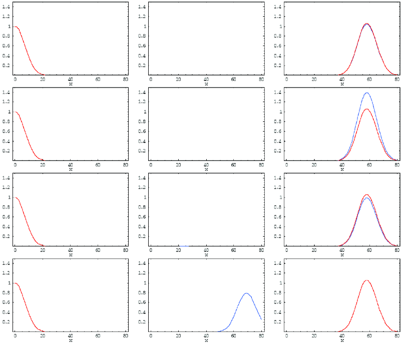
Figure 3.7: Propagation of the electric field $E=<\hat{E}>$ (blu line) with envelope $\exp\{-(x/10)^{2}\}$ for three time slices corresponding to $\theta(t)=0,\ \pi/2,\ 0$, in the case $\eta>0$ ($\gamma_{1}>0$), i.e. amplification without inversion regime; it is also reported the case $\eta=0$ (red line). The mixing angle is rotated from $0$ to $\pi/2$ and back according to $\cot\theta(t)=0.8(1-0.5\tanh[0.1(t-15)]+0.5\tanh[0.1(t-125)])$. By varying the dephasing ($\gamma_{1}$) between the two lower-states, there is a balance between two $\gamma_{1}$-induced effects: the destruction of the EIT window at higher dephasings and the amplification without inversion produced by the population in the level 2. This situation is represented for different values of $\gamma_{1}$ in the range $[0,1]$, in units of $\gamma_{3}$. In agreement with Fig. 2.22, for low values of $\gamma_{1}$ there are unavoidable losses in the process of storing and releasing; indeed the peak of pulse (blu line) is lower than one for $\eta=0$ (red line). For higher dephasing there is gain, that compensates the losses and give also the amplification of dark–state polariton. When increasing more and more $\gamma_{1}$, the dephasing destroy the EIT window, there is absorption and it is no more possible to stop the pulse. Parameters are $g^{2}N=1/100$ and axes are in arbitrary units with $c=1$.

3.6 Decoherence of quantum state transfer

In this section we report some results published in [69] regarding the decoherence effects in the transfer process of a quantum memory. It must be noted that an extension of these results to the case of gain without inversion would be necessary to discuss the possible application to quantum cloning. As already explained this would go beyond the scope of this thesis.

3.6.1 Random spin flips and dephasing

On the level on individual atoms the storage occurs within the two-state system consisting of $|1\rangle$ and $|2\rangle$. If we assume that all other atomic states including $|3\rangle$ are energetically much higher, we may safely neglect decoherence processes involving the excitation of those states. Then decoherence caused by individual and independent reservoir interactions can be described by the action of the two-level Pauli operators

$$X=\rho_{12}+\rho_{21},\enspace Z=\left[\rho_{12},\rho_{21}\right],\enspace Y=i\rho_{12}-i\rho_{21}$$ (3.44)

where $X$ describes a symmetric spin flip of the atom, $Z$ a phase flip, and $Y$ a combination of both. Any single-atom error can be expressed in terms of these and we will restrict the discussion here to the action of $X$ (symmetric spin flip), $X+iY$ (asymmetric spin flip) and $Z$ (phase flip).

Spin flip from $|1\rangle\to|2\rangle$

Consider a quantum memory initially in an ideal storage state, i.e. $\eta=0$. Suppose that an atom then undergoes a spin flip to the internal state $|2\rangle$ if it is initially in state $|1\rangle$. Such a spin flip process could mimic a stored photon.

The authors in [69] have calculated the fidelity of the quantum memory after a single spin flip error, which for the case of an initial pure state $\rho_{0}=|\psi_{0}\rangle\langle\psi_{0}|$ is defined as

$$f\Bigl{(}|\psi_{0}\rangle\Bigr{)}=\langle\psi_{0}|\rho_{1}|\psi_{0}\rangle=\textrm{Tr}\{\rho_{1}\rho_{0}\}$$ (3.45)

where $\rho_{1}$ represent the imperfect final state.

They find for a stored Fock-state $|n\rangle$ with $n\ll N$

$$f_{b\to c}\Bigl{(}|n\rangle\Bigr{)}=\frac{1-\frac{1}{N}}{1-\frac{n}{N}}=1-\frac{n+1}{N}+{\cal O}\left(\frac{1}{N^{2}}\right)$$ (3.46)

while for a coherent state $|\alpha\rangle$ they obtain

$$f_{b\to c}\Bigl{(}|\alpha\rangle\Bigr{)}=\frac{1-\frac{1}{N}+\frac{|\alpha|^{2}}{N}}{1+\frac{|\alpha|^{2}}{N}}=1-\frac{1}{N}+{\cal O}\left(\frac{1}{N^{2}}\right)$$ (3.47)

This reflects the general property of non-classical states to be more sensitive to decoherence than classical ones.

Symmetric spin flip

If instead of the asymmetric spin flip $\rho_{21}=X+iY$ a symmetric flip happens, the authors in [69] find that the fidelity of the memory reads for a stored Fock and coherent state

$$f_{b\leftrightarrow c}(|n\rangle) = 1-\frac{2n+1}{N}+{\cal O}\left(\frac{1}{N^{2}}\right)$$ (3.48)

$$f_{b\leftrightarrow c}(|\alpha\rangle) = 1-\frac{1}{N}+{\cal O}\left(\frac{1}{N^{2}}\right)$$ (3.49)

Phase flip

If after the preparation of an ideal storage state an atom undergoes a phase flip the fidelity is [69]

$$f_{\rm deph}(|\psi_{0}\rangle)=1-\frac{2\langle n\rangle}{N}+{\cal O}\left(\frac{1}{N^{2}}\right)$$ (3.50)

where $\langle n\rangle=\langle\Psi^{\dagger}\Psi\rangle$ is the average number of dark–state polaritons in the initial state. One recognizes that a phase flip of a single atom leads to a fidelity reduction which is of the order of $1/N$. The term $1/N$ again compensates for the fact that in an $N$-atom ensemble the likelihood that one arbitrary atom undergoes a phase flip is $N$ times the probability of a phase flip for a single atom. It is interesting to note that the fidelity only depends on the average dark–state polariton number, i.e. dephasing affects in lowest order of $1/N$ classical and nonclassical states in a similar way.

3.6.2 One-atom losses

Another important source of errors in a collective quantum memory is the loss of an atom from the ensemble.

The fidelity of the quantum memory for a Fock state $|n\rangle$ after loss of a single atom is given by [69]

$$f_{\rm loss}(|n\rangle)=1-\frac{n}{N}$$ (3.51)

The decrease of the fidelity again scales only as $1/N$. This result could of course have been expected as the $n$ excitations are equally distributed over all atoms. Thus removing one reduces the stored information only by the amount $n/N$.

For the case of a general state the fidelity after the loss of an atom reads [69]

$$f_{\rm loss}(|\psi_{0}\rangle)=1-\frac{1}{N}\Bigl{(}\langle\Psi^{\dagger}\Psi\rangle-\langle\Psi^{\dagger}\rangle\langle\Psi\rangle\Bigr{)}+{\cal O}\left(\frac{1}{N^{2}}\right)$$ (3.52)

If the initial storage state corresponds e.g. to a coherent state, the second and third term in (3.52) compensate each other and the fidelity differs from unity only in order $1/N^{2}$. Here again the robustness of classical states becomes apparent.

3.6.3 Atomic motion

Until now it has been assumed that the atoms used in the quantum memory are at a fixed position during the entire storage time. Since the coupling of the atoms to the quantum as well as control fields contains however a spatial phase, see Eq. (3.13), atomic motion results in an effective dephasing and will lead to a reduction of the fidelity. Recently Sun et al. have argued that inhomogeneities of the atom-light interaction strength or in the control field together with atomic motion lead to an increase of the characteristic decoherence rate by a factor $\sqrt{N}$ [70]. In this context the authors in [69] analyze the effect of atomic motion

To reduce the effect of motion in an atomic vapor one could either reduce the temperature or use a buffer gas of sufficient density. In the latter case, which has been used in room temperature gas-cell experiments [13, 25], the free motion is replaced by a diffusion. Therefore now we will restrict the discussion to this important case. Recall that the phase is given by

$$\Delta\phi_{j}(t)\equiv\Delta\vec{k}\cdot\vec{r}_{j}(t)$$ (3.53)

where $\vec{r}_{j}(t)$ denoting the position of the $j$th atom at time $t$ and $\Delta\vec{k}=\vec{k}_{1}-k_{0}\vec{e}_{x}$ is the wavevector difference between control field and quantized mode. The authors in [69] assume that this phase follows a Wiener diffusion process [71]:

$$\frac{{\rm d}}{{\rm d}t}\Delta\phi_{j}(t) = \mu_{j}(t)$$ (3.54)

$$\overline{\,\mu_{j}(t)\,} = 0,$$ (3.55)

$$\overline{\,\mu_{j}(t)\mu_{k}(t^{\prime})\,} = D\delta_{jk}\delta(t-t^{\prime})$$ (3.56)

with $D$ being a characteristic diffusion rate.

In this approach they find the following fidelity of the quantum memory for atomic motion

$$f_{\rm motion}\Bigl{(}|1\rangle\Bigr{)}=\frac{1}{N}\Bigl{(}1+(N-1){\rm e}^{-Dt}\Bigr{)}\sim{\rm e}^{-Dt}$$

A generalization to an arbitrary Fock state $|D,n\rangle$ leads to a fidelity decay proportional to $\exp\{-nDt\}$. One recognizes that the atomic motion causes a decay of the fidelity with a rate given only by the single-atom diffusion rate $D$. In contrast to the results of Sun, Yi and You [70] they find that there is no enhancement of the decay with increasing number of atoms.

All these results play a key role to determine the storage time of these quantum memories and the quantum state transfer fidelity, necessary to decide if that device is or not good for the desired task for which the quantum state is kept.

Chapter 4 Parastatistics in gain medium

4.1 Generalized physical statistics

The notion of statistics is related to the symmetry properties of the wave function of $N$ identical particles, $\psi(1,2,...,N)$, the bosons (fermions) corresponding to symmetric (antisymmetric) wave functions under the exchange of particles; besides in the second quantization scheme the annihilation and creation operators for bosons (fermions) obey the canonical (anti-)commutation relations.

Wigner was the first to remark that the canonical quantization was not the most general quantization scheme consistent with the Heisenberg equations of motions [72]. Parastatistics was so introduced by Green [73] as a general quantization method of quantum field theory different from the canonical Bose and Fermi quantization, by extending the Bose and Fermi statistics [74, 75, 76, 77]. Nevertheless for the long period of time the interest to it was rather academic even if it was closely related with the discovery of color in the context of the theory of strong interactions.

Recently it has found applications in the physics of fractional Hall effect and it probably is relevant to high-Tc superconductivity [78], so it draws more and more attentions from both theoretical and experimental physicists. Indeed the experiments on quantum Hall effect confirm the existence of fractionally charged excitations.

Since the pioneering work of Gentile and Green [73, 79], there have been many extensions beyond the standard statistics, among the others we may list the following: parastatistics, fractional statistics, quon statistics [80], anyon statistics [75, 76, 81] and quantum groups statistics. Note that in the literature there are two principal methods of introducing an intermediate statistical behavior. The first one is to deform the quantum algebra of the commutation-anticommutation relations thus deforming the exchange factor between permuted particles. The second method is based on modifying the number of ways of assigning particles to a collection of states and thus the statistical weight of the many-body system. Here we will refer to the first approach.

In particular in the parastatistics framework the standard bosonic or fermionic fields, which would create identical particles, are replaced by composite fields whose components commute with themselves and anticommute with each other for parabosons, or vice versa for parafermions. The number of components of the fields, $p$, defines the “order” of parastatistics. In general, one can put at most $p$ parafermions in a totally symmetric wavefunction, and at most $p$ parabosons in a totally antisymmetric one. Parastatistics in this approach has been well-studied [82, 83, 84, 85] and the simplest non-trivial representations arise for $p=1$ and coincide with the usual Bose (Fermi) Fock representations.

4.2 Parapolariton in EIT

Let us analyze in detail the effect of the population ($\eta$) in the level $\left.|2\right\rangle$, in the three–level scheme studied in the last chapter, on the commutation relations of the quasi-particles, i.e. on their statistics.

Recall Eq. (3.31) in which the dark–state polariton fields (in the same k-mode) possess the following commutation relations

$$\Bigl{[}\hat{\Psi},\hat{\Psi}^{\dagger}\Bigr{]}=1-2\eta\sin^{2}\theta$$ (4.1)

where $\eta$ is the population in level 2 and $\theta$ is the mixing angle of the polariton.

Eq. (4.1) describe a kind of deformed oscillator or paraboson, because it presents a deviation from the canonical bosonic commutation relations; we call them parapolaritons.

Many kinds of deformed oscillators (parabosons) have been introduced in the literature (see [86] for a list). All of them can be accommodated within the common mathematical framework of the generalized deformed oscillator [87, 88], which is defined as the algebra generated by the operators $\{\hat{1},\hat{a},\hat{a}^{\dagger},\hat{N}\}$ and the structure function $\Phi(x)$, satisfying the relations

$$[\hat{a},\hat{N}]=\hat{a}\qquad[\hat{a}^{\dagger},\hat{N}]=-\hat{a}^{\dagger}$$ (4.2)

$$\hat{a}^{\dagger}\hat{a}=\Phi(\hat{N})=[\hat{N}]\qquad\hat{a}\hat{a}^{\dagger}=\Phi(\hat{N}+\hat{1})=[\hat{N}+\hat{1}]$$ (4.3)

where $\Phi(x)$ is a positive analytic function with $\Phi(0)=0$ and $\hat{N}$ is the number operator. From Eq. (4.3) we conclude that

$$\hat{N}=\Phi^{-1}(\hat{a}^{\dagger}\hat{a})$$ (4.4)

and that the following commutation and anticommutation relations are obviously satisfied:

$$[\hat{a},\hat{a}^{\dagger}]=[\hat{N}+\hat{1}]-[\hat{N}]\qquad\{\hat{a},\hat{a}^{\dagger}\}=[\hat{N}+\hat{1}]+[\hat{N}]$$ (4.5)

The structure function $\Phi(x)$ is characteristic to the deformation scheme. In Table 4.1 the structure functions corresponding to different deformed oscillators are given.

It can be proved that the generalized deformed algebras possess a Fock space of eigenvectors $\left.|0\right\rangle,\left.|1\right\rangle,\ldots,\left.|n\right\rangle,\ldots$ of the number operator $\hat{N}$

$$\hat{N}\left.|n\right\rangle=n\left.|n\right\rangle\quad\langle n\left.|m\right\rangle=\delta_{nm}$$ (4.6)

if the vacuum state $\left.|0\right\rangle$ satisfies the following relation:

$$\hat{a}\left.|0\right\rangle=0$$ (4.7)

These eigenvectors are generated by the formula:

$$\left.|n\right\rangle{1\over\sqrt{[n]!}}{\left(\hat{a}^{\dagger}\right)}^{n}\left.|0\right\rangle$$ (4.8)

where

$$[n]!=\prod_{k=1}^{n}[k]=\prod_{k=1}^{n}\Phi(k)$$ (4.9)

The generators, $\hat{a}^{\dagger}$ and $\hat{a}$, are the creation and annihilation operators of this deformed oscillator algebra:

$$\hat{a}\left.|n\right\rangle=\sqrt{[n]}\left.|n-1\right\rangle\qquad\hat{a}^{\dagger}\left.|n\right\rangle=\sqrt{[n+1]}\left.|n+1\right\rangle$$ (4.10)

These eigenvectors are also eigenvectors of the energy operator

$$\hat{H}={\hbar\omega\over 2}(\hat{a}\hat{a}^{\dagger}+\hat{a}^{\dagger}\hat{a})$$ (4.11)

corresponding to the eigenvalues

$$E(n)={\hbar\omega\over 2}(\Phi(n)+\Phi(n+1))={\hbar\omega\over 2}([n]+[n+1])$$ (4.12)

For $\Phi(n)=n$ one obtains the results for the ordinary harmonic oscillator. Besides in this generalized framework we can define two new operators, $\hat{b}$ and $\hat{b}^{\dagger}$

$$\hat{b}=\hat{a}\sqrt{\frac{n}{\phi(n)}}\ \ \ \ \ \ \ \ \ \ \ \ \hat{b}^{\dagger}=\hat{a}^{\dagger}\sqrt{\frac{n}{\phi(n)}}$$ (4.13)

that obey the canonical bosonic commutation relations, as one can easily show; indeed $[\hat{b},\hat{b}^{\dagger}]=1$. According to Eq. (4.1), $\Phi(n)=n(1-2\eta\sin^{2}{\theta})$ with $0\leq\eta<1/2$; this restriction in $\eta$ is justified by the requirement that $\phi(x)$ is a positive analytic function. By this definition of $\phi$, we have

$$\Bigl{[}\hat{\Psi},\hat{\Psi}^{\dagger}\Bigr{]}=(1-2\eta\sin^{2}\theta)$$ (4.14)

and the eigenvalues are:

$$E(n)={\hbar\omega\over 2}(\Phi(n)+\Phi(n+1))=\hbar\omega\Big{(}n+\frac{1}{2}\Big{)}(1-2\eta\sin^{2}\theta)$$ (4.15)

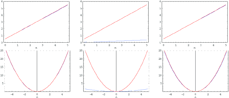
Figure 4.1: Top: the energy of the deformed boson oscillator (blu line), $E(n)$, as function of $n$ for three time slices corresponding to $\theta(t)\simeq 0,\ \pi/2,\ 0$, in units of $\hbar\omega$. During the stopping of light the ideal bosonic spectrum (red line) is compressed and when releasing the photon the bosonic energy width is recovered. There is a mapping from bosons to fermions described by the compression of bosonic energy spectrum to a fermionic 2-level one. The narrowing of energy spacing reflects the Pauli principle and an effective repulsive interaction that describes the mapping bosons–fermions. Bottom: the relative effective potential, $V(x)$, is reported according to the results above.

When a dark–state polariton propagates through a three–level atomic system, there is a mapping from bosons to fermions. Indeed, at the beginning, when the pump field $\Omega_{P}$ is turned on, the polariton has only a photonic component and it is a boson. Afterwards, when turning off the pump frequency, the quantum state encoded in photon is converted to spin eccitation of atoms. In other words, during the stopping of light, the dark–state polariton has only spin-atomic component and so it is a fermion. In the intermediate time the polariton obey to a particular parastatistics, as deformed harmonic oscillator.

In terms of energy, during the stopping of light the ideal bosonic spectrum is compressed and it recovers the original energy width during the release of photon. There is a mapping from bosons to fermions described by the compression of bosonic energy spectrum to a fermionic 2-level one. The narrowing of energy spacing reflects the Pauli principle and an effective repulsive interaction that describes the mapping bosons–fermions. In other words the commutation relations in Eq. (3.31) resemble bosonic commutation relations but in addition include corrections due to the presence of the Pauli principle.

Table 4.1: Structure functions of special deformation schemes

	$\Phi(x)$	Reference
i	$x$	harmonic oscillator, bosonic algebra
ii	${{q^{x}-q^{-x}}\over{q-q^{-1}}}$	$q$-deformed harmonic oscillator [91, 92]
iii	${{q^{x}-1}\over{q-1}}$	Arik–Coon, Kuryshkin, or $Q$-deformed oscillator [93, 94]
iv	${{q^{x}-p^{-x}}\over{q-p^{-1}}}$	2-parameter deformed oscillator [95, 96, 97]
v	$x(p+1-x)$	parafermionic oscillator [74]
vi	${\sinh(\tau x)\sinh(\tau(p+1-x))}\over{\sinh^{2}(\tau)}$	$q$-deformed parafermionic oscillator [98, 99]
vii	$x\cos^{2}(\pi x/2)+(x+p-1)\sin^{2}(\pi x/2)$	parabosonic oscillator [74]
viii	$\begin{array}[]{c}\frac{\sinh(\tau x)}{\sinh(\tau)}\frac{\cosh(\tau(x+2N_{0}-1))}{\cosh(\tau)}\cos^{2}(\pi x/2)+\\ +\frac{\sinh(\tau(x+2N_{0}-1))}{\sinh(\tau)}\frac{\cosh(\tau x)}{\cosh(\tau)}\sin^{2}(\pi x/2)\end{array}$	$q$-deformed parabosonic oscillator [98, 99]
ix	$\sin^{2}{\pi x/2}$	fermionic algebra [100]
x	$q^{x-1}\sin^{2}{\pi x/2}$	$q$-deformed fermionic algebra [101, 102, 103, 104, 105, 106]
xi	$\frac{1-(-q)^{x}}{1+q}$	generalized $q$-deformed fermionic algebra [107]
xii	$x^{n}$	[87]
xiii	${{sn(\tau x)}\over{sn(\tau)}}$	[87]

Chapter 5 Polarization quantum memory

Up to now we have analyzed a quantum memory for the number of photons. Indeed the information that is conserved in the quantum memory studied above is the number of photons, converted into the number of collective spin excitations. Actually in quantum information science many protocols need two–level quantum system or qubit and, because the most of implementations use the photons as ideal carriers of information, the quantum information is encoded in some physical freedom degrees of a photon, i.e its polarization. For example we can use the two polarizations, $\sigma_{+}$ and $\sigma_{-}$, to encode two orthogonal quantum states, i.e. to treat a photon as a qubit.

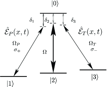
Figure 5.1: Energy level scheme for a tripod. Detunings $\delta_{j}=\omega_{0}-\omega_{j}-\omega_{j}^{(L)}$ denote the laser frequency ($\omega_{j}^{(L)}$) detunings from the respective transitions $|j\rangle\leftrightarrow|0\rangle$. States $|1\rangle$, $|2\rangle$ and $|3\rangle$ correspond to the states $|5S_{1/2},F=1,m=\{-1,0,1\}\rangle$ of ⁸⁷Rb, while state $|0\rangle=|5P_{3/2},F=0\rangle$. [108]

For this reason now we examine a four-level atomic tripod configuration in Fig. 5.1, already studied in [108] for quantum phase gate (off–resonance). This has often been used as an extension of a $\Lambda$ scheme, e.g. by Paspalakis who suggested its potential for nonlinear optical processes [109]. It should be mentioned that while Paspalakis considered the case of a single weak probe, the authors in [108] adopt a setup with two weak fields namely a $probe$ and a $trigger$ in the presence of a strong pump that creates EIT.

The advantage of this scheme is that the two probe, $\hat{\cal E}_{P}(x,t)$ and $\hat{\cal E}_{T}(x,t)$, have different polarization, i.e. $\sigma_{+}$ and $\sigma_{-}$. In such a way, we so introduced a quantum memory for polarized photons. This kind of quantum memory has been investigated only in cavity QED and proposed recently by Lukin and Fleischhauer in a different atomic scheme [23]. Then the proposal of this thesis would represent a new interesting polarization quantum memory for light, useful in different quantum information protocols.

5.1 EIT effect in a Tripod System

The energy level scheme of a tripod system is given in Fig. 5.1. Probe and trigger fields have Rabi frequencies $\Omega_{P}$ and $\Omega_{T}$ and polarizations $\sigma_{+}$ and $\sigma_{-}$. The pump Rabi frequency is $\Omega$.

Among the four eigenstates in the system two contain no contribution from the excited state $|0\rangle$ and hence they are dark states [110]. For the special case of atomic detunings $\delta_{j}=\delta=0$, these are

$$|e_{1}\rangle = \frac{\Omega_{T}|1\rangle-\Omega_{P}|3\rangle}{\sqrt{\Omega_{P}^{2}+\Omega_{T}^{2}}}$$ (5.1)

$$|e_{2}\rangle = \frac{\Omega\Omega_{P}|1\rangle+\Omega\Omega_{T}|3\rangle-\left(\Omega_{P}^{2}+\Omega_{T}^{2}\right)|2\rangle}{\sqrt{\left(\Omega_{P}^{2}+\Omega_{T}^{2}\right)\left(\Omega_{P}^{2}+\Omega^{2}+\Omega_{T}^{2}\right)}}$$ (5.2)

The two other states (bright states)

$$|e_{\pm}\rangle=\frac{\Omega_{P}|1\rangle\pm|0\rangle+\Omega_{T}|3\rangle+\Omega|2\rangle}{\sqrt{\Omega_{P}^{2}+\Omega^{2}+\Omega_{T}^{2}}}$$ (5.3)

contain $\left.|0\right\rangle$ and have energies $\pm\sqrt{\Omega_{P}^{2}+\Omega^{2}+\Omega_{T}^{2}}$.

The atomic evolution is governed by a set of Heisenberg-Langevin equations (including atomic spontaneous emission and dephasing)

$$i\dot{\rho}_{00} = -i(\gamma_{11}+\gamma_{22}+\gamma_{33})\rho_{00}+\Omega_{P}^{*}\rho_{10}-\Omega_{P}\rho_{01}$$

$$+\Omega^{*}\rho_{20}-\Omega\rho_{02}+\Omega_{T}^{*}\rho_{30}-\Omega_{T}\rho_{03}$$

$$i\dot{\rho}_{11} = i\gamma_{11}\rho_{00}+i\gamma_{12}\rho_{22}+i\gamma_{13}\rho_{33}+\Omega_{P}\rho_{01}-\Omega_{P}^{*}\rho_{10}$$

$$i\dot{\rho}_{22} = i\gamma_{22}\rho_{00}-i\gamma_{12}\rho_{22}+i\gamma_{23}\rho_{33}+\Omega\rho_{02}-\Omega^{*}\rho_{20}$$

$$i\dot{\rho}_{33} = i\gamma_{33}\rho_{00}-i(\gamma_{13}+\gamma_{23})\rho_{33}+\Omega_{T}\rho_{03}-\Omega_{T}^{*}\rho_{30}$$

$$i\dot{\rho}_{10} = -\Delta_{10}\rho_{10}+\Omega_{P}\rho_{00}-\Omega_{P}\rho_{11}-\Omega\rho_{12}-\Omega_{T}\rho_{13}$$ (5.4)

$$i\dot{\rho}_{20} = -\Delta_{20}\rho_{20}+\Omega\rho_{00}-\Omega\rho_{22}-\Omega_{P}\rho_{21}-\Omega_{T}\rho_{23}$$

$$i\dot{\rho}_{30} = -\Delta_{30}\rho_{30}+\Omega_{T}\rho_{00}-\Omega_{T}\rho_{33}-\Omega_{P}\rho_{31}-\Omega\rho_{32}$$

$$i\dot{\rho}_{12} = -\Delta_{12}\rho_{12}+\Omega_{P}\rho_{02}-\Omega^{*}\rho_{10}$$

$$i\dot{\rho}_{13} = -\Delta_{13}\rho_{13}+\Omega_{P}\rho_{03}-\Omega_{T}^{*}\rho_{10}$$

$$i\dot{\rho}_{23} = -\Delta_{23}\rho_{23}+\Omega\rho_{03}-\Omega_{T}^{*}\rho_{20}$$

where the decay rates $\gamma_{ij}$ describe decay of populations and coherences, $\Delta_{j0}=\delta_{j}+i\gamma_{j0}$ and $\Delta_{ij}=\delta_{j}-\delta_{i}-i\gamma_{ij}$, with $i,j=1,2,3$.

When all detunings $\delta_{j}$ are vanishing (on resonance), probe and trigger share a strong control field with Rabi frequency $\Omega$ and exhibit all effects associated with ideal EIT including strong group velocity reductions. In this regime the system behaves as a perfect polarization quantum memory for two independent pulses. Indeed if a probe (trigger) field propagates into this medium then the polarization $\sigma^{+}$ ($\sigma^{+}$) is mapped to atomic spin-excitation. Besides when a photon in any polarization state enters upon this memory, also this superposition of $\sigma^{+}$ and $\sigma^{-}$ is saved in this quantum register because, for perfectly equal detunings degeneracy, there is a common transparency window for both fields and our tripod system is linear [108]. Therefore, apart from the quantum memories analyzed in the last chapters, here with this four-level configuration any quantum state of a polarized photon is coherently memorized.

In order to verify this ideal EIT effect in presence of two fields, now we consider the steady state solutions to the Bloch equations. When $|\Omega|^{2}\gg|\Omega_{P,T}|^{2}$ and $\Omega_{P}\approx\Omega_{T}$, the steady-state population distribution will be symmetric with respect to the $1\leftrightarrow 3$ exchange, i.e. $\rho_{11}\approx\rho_{33}\approx\frac{1}{2}$, with vanishing population in the other two levels. This population assumption allows to decouple the equations for the populations from those of the coherences and to obtain the steady state solution. In the following we show the steady-state expression for $\rho_{10}$:

$$\frac{\left(\rho_{10}\right)_{ss}}{\Omega_{P}} = \left(1+\frac{1}{4}\frac{\left(\Delta_{12}\Delta_{23}/\Delta_{13}^{2}\right)|\Omega_{P}|^{2}|\Omega_{T}|^{2}}{\left(\Delta_{10}\Delta_{12}-|\Omega|^{2}\right)\left(\Delta_{30}^{*}\Delta_{23}-|\Omega|^{2}\right)}\right)^{-1}$$ (5.5a)

$$\times \left\{-\frac{1}{2}\frac{\Delta_{12}\Delta_{13}}{\Delta_{10}\Delta_{12}\Delta_{13}-\Delta_{13}|\Omega|^{2}-\Delta_{12}|\Omega_{T}|^{2}}\right.$$

$$\left.-\frac{1}{2}\frac{\Delta_{12}\Delta_{13}\Delta_{23}|\Omega_{T}|^{2}}{\Delta_{30}^{*}\Delta_{13}\Delta_{23}-\Delta_{13}|\Omega|^{2}-\Delta_{23}|\Omega_{P}|^{2}}\right\}$$

In Fig. 5.2 we report the real and imaginary part of $\rho_{10}$ when the pump field is on the resonance. When the trigger field is also on the resonance, the system is linear, there is no dephasing between the two field and an ideal EIT regime for both of pulses: in these conditions we propose the polarization quantum memory. Instead, when there is a mismatch between the detunings, an effective Kerr non-linearity appears [108].

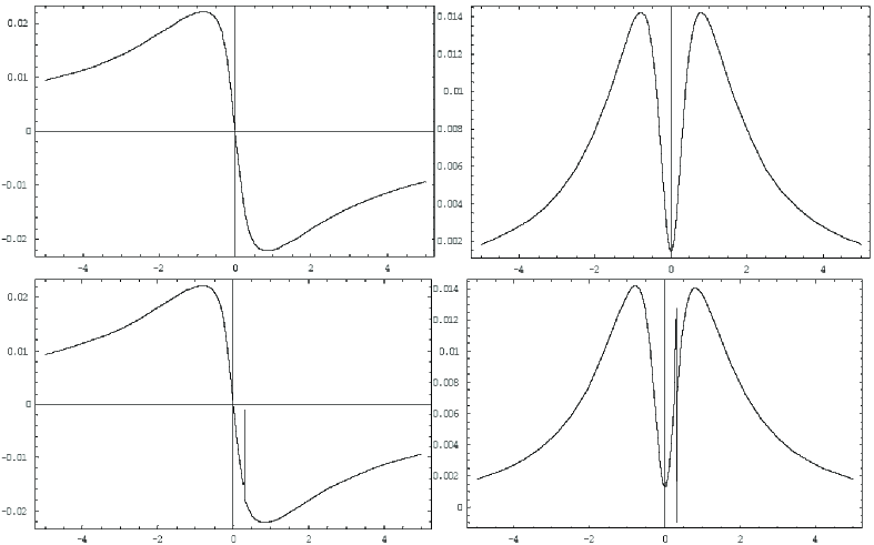
Figure 5.2: Real (left) and imaginary (right) part of $\rho_{10}$ are reported when the pump field is on the resonance. In the top the trigger field is also on the resonance and then the system is linear, there is no dephasing between the two field and an ideal EIT regime for both of pulses. In the bottom we analyze the situation in which there is a mismatch between the detunings and a cross-phase modulation appears [108]. Indeed the probe detuning dependence of $\rho_{10}$ is perturbed by this off–resonance Kerr non-linearity.

5.2 Scattering of dark–state polaritons

Let us consider the case in which probe and trigger are quantum fields. The pump is still considered much stronger than both of them so as to neglect its quantum fluctuations as for a classical field. We specifically adopt a recently developed formalism [65, 111, 27] and apply it to our tripod atomic configuration. The relevant interaction Hamiltonian is

$$H_{int} = -\int\frac{dz}{L}N\left[\hbar\delta_{1}\rho_{00}+\hbar(\delta_{1}-\delta_{2})\sigma_{22}+\hbar(\delta_{1}-\delta_{3})\rho_{33}\right.$$

$$+\hbar g_{P}\left(\hat{{\cal E}}_{P}\rho_{01}+\hat{{\cal E}}_{P}^{\dagger}\rho_{10}\right)+\hbar g_{T}\left(\hat{{\cal E}}_{T}\rho_{03}+\hat{{\cal E}}_{T}^{\dagger}\rho_{30}\right)\left.+\hbar\Omega(\rho_{02}+\rho_{20})\right]$$

where $L$ is the interaction length along the propagation axis $x$, $g_{P,T}$ denotes coupling strengths of probe and trigger fields $\hat{{\cal E}}_{P,T}$ to the respective atomic transitions, and $\rho_{ij}=\frac{1}{N}\sum_{k}\rho_{ij}^{(k)}$ are the collective operators for the atomic populations and transitions for $N$ atoms in a medium. The equations for probe and trigger pulses propagating along $x-$axis through the tripod-media are given by

$$\left(\frac{\partial}{\partial t}+c\frac{\partial}{\partial x}\right)\hat{{\cal E}}_{P}(x,t) = ig_{P}N\rho_{10}$$ (5.6)

$$\left(\frac{\partial}{\partial t}+c\frac{\partial}{\partial x}\right)\hat{{\cal E}}_{T}(x,t) = ig_{T}N\rho_{30}$$ (5.7)

while the equations for atomic transition operators (with all detunings vanishing) are

$$\dot{\rho}_{10} = -\gamma_{10}\rho_{10}+ig_{P}\hat{{\cal E}}_{P}(\rho_{11}-\rho_{00})+ig_{T}\hat{{\cal E}}_{T}\rho_{13}+i\Omega\rho_{12}$$

$$\dot{\rho}_{20} = -\gamma_{20}\rho_{20}+ig_{P}\hat{{\cal E}}_{P}\rho_{21}+ig_{T}\hat{{\cal E}}_{T}\rho_{23}+i\Omega(\rho_{22}-\rho_{00})$$

$$\dot{\rho}_{30} = -\gamma_{30}\rho_{30}+ig_{P}\hat{{\cal E}}_{P}\rho_{31}+ig_{T}\hat{{\cal E}}_{T}(\rho_{33}-\rho_{00})+i\Omega\rho_{32}$$ (5.8)

$$\dot{\rho}_{12} = -\gamma_{12}\rho_{12}-ig_{P}\hat{{\cal E}}_{P}\rho_{02}+i\Omega\rho_{10}$$

$$\dot{\rho}_{13} = -\gamma_{13}\rho_{13}-ig_{P}\hat{{\cal E}}_{P}\rho_{03}+ig_{T}\hat{{\cal E}}_{T}^{\dagger}\rho_{10}$$

$$\dot{\rho}_{23} = -\gamma_{23}\rho_{23}+ig_{T}\hat{{\cal E}}_{T}^{\dagger}\rho_{20}-i\Omega\rho_{03}$$

where $\gamma_{\mu\nu}$ are the relative dephasing between the levels $\left.|\mu\right\rangle$ and $\left.|\nu\right\rangle$.

We now proceed by assuming the low intensity probe and trigger, $g_{j}\langle\hat{{\cal E}}_{P,T}\rangle\ll\Omega$ and strong pump $|\Omega|^{2}/\gamma_{0j}\gamma_{ij}\gg 1$. The latter condition also implies that the EIT resonances for both, probe and trigger fields, are strongly saturated. Furthermore, if $g_{P}\sim g_{T}\sim g$, for a probe and trigger fields of equal mean amplitudes $\langle\hat{{\cal E}}\rangle$, we can assume $\langle\rho_{00}\rangle\approx\langle\rho_{22}\rangle\approx 0$ and $\langle\rho_{11}\rangle\approx\langle\rho_{33}\rangle\approx\frac{1}{2}$.

Besides, following the procedure in chapter 3, in the low-intensity approximation we have

$$\rho_{10}=-\frac{i}{\Omega}\frac{\partial}{\partial t}\rho_{12}$$ (5.9)

$$\rho_{30}=-\frac{i}{\Omega}\frac{\partial}{\partial t}\rho_{32}$$ (5.10)

Hence in the adiabatic limit one finds

$$\rho_{12}=-\frac{g}{\Omega}\Big{[}\frac{\hat{{\cal E}}_{P}}{2}+\hat{{\cal E}}_{T}\rho_{13}\Big{]}$$ (5.11)

$$\rho_{32}=-\frac{g}{\Omega}\Big{[}\frac{\hat{{\cal E}}_{T}}{2}+\hat{{\cal E}}_{P}\rho_{31}\Big{]}$$ (5.12)

Therefore one arrives at the equations for the pulse propagation

$$\left(\frac{\partial}{\partial t}+c\frac{\partial}{\partial x}\right)\hat{{\cal E}}_{P}(x,t) \cong -\frac{{g}^{2}N}{\Omega}\frac{\partial}{\partial t}\Big{[}\frac{\hat{{\cal E}}_{P}}{2\Omega}+\frac{\hat{{\cal E}}_{T}}{\Omega}\rho_{13}\Big{]}$$ (5.13)

$$\left(\frac{\partial}{\partial t}+c\frac{\partial}{\partial x}\right)\hat{{\cal E}}_{T}(x,t) \cong -\frac{{g}^{2}N}{\Omega}\frac{\partial}{\partial t}\Big{[}\frac{\hat{{\cal E}}_{T}}{2\Omega}+\frac{\hat{{\cal E}}_{P}}{\Omega}\rho_{31}\Big{]}$$ (5.14)

where

$$\rho_{13}=-\gamma_{13}\rho_{13}-\frac{\hat{{\cal E}}_{P}}{N}\left(\frac{\partial}{\partial t}+c\frac{\partial}{\partial x}\right)\hat{{\cal E}}_{T}(x,t)-\frac{\hat{{\cal E}}_{T}}{N}\left(\frac{\partial}{\partial t}+c\frac{\partial}{\partial x}\right)\hat{{\cal E}}_{P}(x,t)$$

Note that the Eqs. (5.13-5.14) emphasize the full symmetry between the probe and the trigger dynamics, a symmetry which is intimately linked with the atomic population being equally distributed between levels $\left.|1\right\rangle$ and $\left.|3\right\rangle$. Besides in the regime considered here the coupling between two fields is substantially zero. Therefore two field propagates through atomic system independently.

Let us introduce again a rotation in the space of physically relevant variables – the electric field $\hat{\cal E}$ and the atomic spin coherences – defining four new quantum fields $\hat{\Psi}_{1}(x,t)$, $\Phi_{1}(x,t)$ for the probe and $\Psi_{2}(x,t)$ and $\Phi_{2}(x,t)$ for the trigger field, as follows

$$\hat{\Psi}_{1}(x,t) = \cos\theta(t)\,\hat{\cal E}_{P}(x,t)-\sin\theta(t)\,\sqrt{N}\,\rho_{10}(x,t)\,{\rm e}^{i\Delta kx}$$ (5.15)

$$\hat{\Phi}_{1}(x,t) = \sin\theta(t)\,\hat{\cal E}_{P}(x,t)+\cos\theta(t)\,\sqrt{N}\,\rho_{10}(x,t)\,{\rm e}^{i\Delta kx}$$ (5.16)

$$\hat{\Psi}_{2}(x,t) = \cos\theta(t)\,\hat{\cal E}_{T}(x,t)-\sin\theta(t)\,\sqrt{N}\,\rho_{30}(x,t)\,{\rm e}^{i\Delta kx}$$ (5.17)

$$\hat{\Phi}_{2}(x,t) = \sin\theta(t)\,\hat{\cal E}_{T}(x,t)+\cos\theta(t)\,\sqrt{N}\,\rho_{30}(x,t)\,{\rm e}^{i\Delta kx}$$ (5.18)

where the mixing angle $\theta(t)$ is defined as

$$\tan^{2}\theta(t)=\frac{g^{2}N}{\Omega^{2}(t)}$$ (5.19)

In the low-intensity approximation and in the adiabatic limit, we obtain (as for one three–level system) these two PDE’s

$$\left[\frac{\partial}{\partial t}+c\cos^{2}\theta(t)\frac{\partial}{\partial x}\right]\hat{\Psi}_{1}(x,t)=0\qquad\left[\frac{\partial}{\partial t}+c\cos^{2}\theta(t)\frac{\partial}{\partial x}\right]\hat{\Psi}_{2}(x,t)=0$$

that describe the propagations of the two polaritons associated to two polarized photons, i.e. with $\sigma_{-}$ and $\sigma_{+}$ polarization.

Therefore it confirms that this system represents a good tool to realize a polarization quantum memory for photons. Moreover, as seen in chapter 3, by turning on two incoherent RF field ($\gamma_{1}^{(1)}$ and $\gamma_{1}^{(2)}$) we can put population in the level 2 and have amplification without inversion to compensate the unavoidable losses. So perhaps it would be possible to obtain also a quantum (continuous-variable) cloning of a quantum state of polarized photons into a quantum memory. However, the relative fidelity of cloning process will be less than one according to No-Cloning Theorem (see A.4).

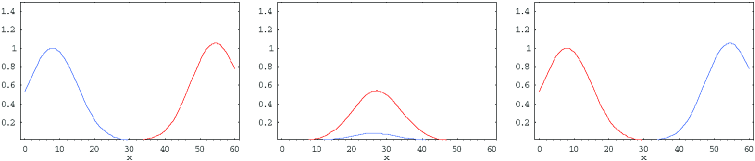
Figure 5.3: Scattering between two dark–state polaritons. Propagation of the electric fields, ${\cal E}_{P}=<\hat{\cal E}_{P}>$ (blu line) and ${\cal E}_{T}=<\hat{\cal E}_{T}>$ (red line), with envelope $\exp\{-(x/10)^{2}\}$ for three time slices corresponding to $\theta(t)=0,\ 3\pi/7,\ 0$, in ideal EIT regime. The mixing angle is rotated from $0$ to $\pi/2$ and back according to $\cot\theta(t)=0.8(1-0.5\tanh[0.1(t-15)]+0.5\tanh[0.1(t-125)])$. Parameters are $g^{2}N=1/100$ and axes are in arbitrary units with $c=1$.

In Fig. 5.3 we show the scattering between two DSP in this tripod configuration and we show that they present a solitonic behavior, i.e. they propagate unperturbed in polarization quantum memory. Let us point out that off-resonance and in presence of a detuning mismatch a relative phase between two dark state polaritons appears, as shown for polarization quantum phase gate in [108]. Then in different regimes this nice system behaves as or quantum phase gate or polarization quantum memory.

Conclusions and Outlook

In this thesis we have investigated some proposals for quantum memories by analyzing the propagation of a coherent light pulse through a three-level atomic system. Under particular conditions we have showed that it is possible to obtain anomalous and retarded light propagation and that a very slow propagation involves a very large amplification of a probe field. This achievement is based on the phenomenon of electromagnetically induced transparency (EIT), which leads to steep normal dispersion of the medium accompanied by vanishing absorption.
EIT happens for a weak probe field resonant or quasi-resonant with an atomic transition when a strong drive field is applied to an adjacent atomic transition under condition of two–photon resonance. Therefore ultraslow light propagation is possible when the two–photon atomic coherence decays much slower than one-photon coherence. This behavior is similar to that of a pulse propagating in any “two–level” dispersive medium and it can be explained in terms of polaritonic modes. However, unlike usual polaritons, almost no energy is stored in the coherent media where ultraslow light is observed. Instead, the coherent media work as a transducer between a slow light pulse and coupling electromagnetic wave.

Ultraslow light and atomic coherence have already found many important applications in low-intensity nonlinear optics and metrology. Novel applications in quantum nonlinear optics and quantum information processing seem to be feasible. Indeed, for example, the coherence allows one to store information about the probe light and transport it in space. It allows time reversing of the light and allows one to increase coupling between light fields such that it becomes possible to study the interaction between single photons. There are a lot of new applications of this coherence and the list is growing fast.

Here, in particular, we have discussed how to couple the light to an atomic system, i.e. a dense gas of three–level atoms, and to imprint the information carried by the photons onto the atoms, specifically as a coherent pattern of atomic spins. This procedure is reversible and the information stored in the atomic spins can later be transferred back to the light field, reconstituting the original pulse. In this context we have analyzed the propagation of a quantum field in an EIT medium sustaining “dark state polaritons” in the quasi-particle picture; then we have studied the decoherence effects in this quantum memory for photons, by recalling some results about the fidelity of the quantum state transfer. We have shown how it is possible to extend the DSP concept in presence of inversionless gain. In this novel regime we have also discussed the possibility of simulating parastatistics showing how the bosonic spectrum is compressed while being mapped onto a fermionic spin $1/2$ system.

Besides we have introduced a polarization quantum memory for photons in EIT regime, by using a four–level atomic configuration, and investigated the DSP solitonic behavior in the scattering of two dark–state polaritons in a tripod atomic configuration.

As regards the experimental implementations of these ideas, an intriguing question is whether EIT effects can be induced in solid state media. In general the high dephasing rates in solid state systems will prevent the development of strong coherence unless a large coupling, sufficiently large that it may risk causing optical damage to the medium, is employed. Given this limitation it remains to be seen how solid state EIT effects can be further developed. To an extent the beauty of EIT is that it leads to exceptionally high efficiency non-linear optical processes and potentially high gains (non-inverted) in a gas phase medium. The high nonlinear conversion efficiencies are of a magnitude normally associated with non-linear frequency mixing in optical crystals. Thus a renewed interest in gas phase non-linear optical devices, possessing unique capabilities (e.g. high conversion efficiencies into the XUV and far-IR), seems likely.

Important potential applications such as quantum communications over long distances might be implemented by combining an EIT-based memory with linear optical elements. Moreover quantum information processing with continuous variables represents an interesting alternative to the traditional qubit-based approach. Indeed, regarding quantum communication applications, as for example quantum teleportation [4] or quantum key distribution (QKD) [112], continuous variables (CV) are particularly promising. Another important feature of CV is the feasibility of the light-atoms quantum interface [113, 11], which unlike its qubit analogue does not require strongly coupled cavity QED regime for deterministic operations. For these reasons, the idea of a quantum memory for light with macroscopic atomic ensembles has been explored in the last years [30, 31, 32, 114]. Such a quantum memory is crucial for applications such as quantum repeaters or quantum secret sharing.

In this field macroscopic atomic ensemble could be also a good tool to realize an optimal cloning machine. We have mentioned that it could be possible realize a quantum cloning into a quantum memory, but in the same device, by using the amplification in an EIT medium.

Finally let us cite an other important application of a quantum memory: quantum cryptography. In the field of quantum information, quantum key distribution (QKD) is the application which is more developed, to the point that already commercial prototypes exist. This fact is a good indicator of just how much attention the subject has received in the last years. In this field it would be interesting implement experimentally an optimal eavesdropping strategy in a quantum channel between two communication agents, Alice and Bob [115]. If the cloning is used as an eavesdropping attack, then the eavesdropper, Eve, would like to store her clone in the memory while the second clone should be sent as a light pulse down the communication line. Afterwards Eve needs to transfer one of the clones from the atomic memory back to light in order to extract the maximal information by a von Neumann measurement of the quantum state, encoded in photon. In this context the quantum memory for polarized photons play a key role for implementing some QKD schemes and for testing the theoretical security of the quantum key distribution protocols, necessary in our global communication era.

Appendix A Appendix

A.1 Lasing without inversion

A laser is a light source that produces a beam of highly coherent and very nearly monochromatic light as result of cooperative emission from many atoms. The name laser is an acronym for light amplification by stimulated emission of radiation [116]. The main ingredients for a laser are an optical cavity and “gain medium”, i.e. a system capable of amplifying electromagnetical radiation. When we think of gain media, we automatically associate stimulated emission and population inversion with the lasing process. Both of these processes are considered necessary in order to accomplish “light amplification”; indeed all traditional laser systems require a population inversion because the probability of an initially unexcited atom absorbing a photon is equal to the probability of stimulated emission from an excited atom [A.1.1]. As a result we need to create a non-equilibrium situation in which the number of atoms in a higher-energy state is greater than the number in the lower-energy state, such a situation is called population inversion. Then the rate of energy radiation by stimulated emission can exceed the rate of absorption and the system acts as a net source of radiation. The photons being the result of stimulated emission have all the same frequency, phase, polarization and direction of propagation. Hence the resulting radiation is much more coherent than the light form ordinary sources. From this argument it would be acceptable to suggest that, without a population inversion, lasing would be impossible. Is it really true?

More to the point we need an atom that is more likely to emit radiation than absorb it. This is where the effect of EIT and the huge benefits of it come into play. Therefore it is possible to lase without population inversion (LWI) in EIT regime. Nevertheless it is noted that although lasing is achieved without requiring an inversion of the population, another laser has to be used in order to achieve this result. With relevance to existing experiments not a lot has been gained but, for the future, a number of exciting possibilities and opportunities have been opened up.

The advantages of lasing without inversion are

• Much lower power pump beams required.

• Transitions which normally shouldn’t lase can be made to lase.

• X-Ray and XUV resonant transitions can be made to lase.

Finally, one could make to laser transitions at short wavelengths, which is impossible with existing systems. This is due to the fact that it is very difficult to create population inversions at X-ray wavelengths (below 200nm) as result of the rapid decay of the excited states via spontaneous emission. However using EIT and quantum interference ideas an alternative may be discovered with the eventual goal of a conventional laser working at X-ray wavelengths.

A.1.1 Einstein’s coefficients

At the beginning of the century, the combination of Bohr’s atomic model with a stochastic conception of the light-matter interaction allowed Einstein to establish the existence of three basic processes in the interaction of light with matter: absorption, stimulated emission and spontaneous emission. In the context of black-body radiation and from thermodynamical arguments, Einstein determined (in terms referred to as Einstein A and B coefficients) the relationship between the rates of absorption and stimulated emission of light by a gas molecule possessing discrete energy levels and the spontaneous emission rate (given by the Einstein A coefficient). For a two-level system with ground level $|g\rangle$ and excited level $|e\rangle$ with unperturbed transition frequency $\omega$ probed by an electromagnetic field, the relationships between the Einstein coefficients read

$$B_{abs}=B_{est}$$ (A.1)

$$\frac{A}{B}=\frac{\hbar\omega^{3}}{\pi^{2}c^{3}}$$ (A.2)

with

$$A=\frac{\omega^{3}}{3\pi\epsilon_{0}\hbar c^{3}}|\mu|^{2}$$ (A.3)

where $\mu$ is the electric dipole moment of the two-level transition, $\hbar$ Planck’s constant, $\epsilon_{0}$ the vacuum electric permittivity, and $c$ the speed of light in vacuum. Thus, the rates of absorption and stimulated emission of light by an atomic/molecular medium will be proportional to the corresponding Einstein B coefficient times the population $\rho_{ii}\leavevmode\nobreak\ (i=g,e)$ of the initial state of the process. Then,

$$\frac{absorption\cdot rate}{stimulated\cdot emission\cdot rate}=\frac{B_{abs}}{B_{est}}\frac{\rho_{gg}}{\rho_{ee}}$$ (A.4)

From the above equations, it can be deduced straightforwardly that since $B_{abs}=B_{est}$, then population inversion, i.e. $\rho_{ee}>\rho_{gg}$, is a necessary condition for light amplification and it is not possible to invert a two-level system with, for instance, resonant light, since atomic excitation is always accompanied with de-excitation through the stimulated emission process. As a consequence, in order to create the required population inversion, laser systems operate on three- or more level configurations (i.e. the three–level configuration of the Ruby laser or the four-level configuration of the He-Ne laser), where the inversion is created by pumping to an excited level which rapidly decays to the upper level of the lasing transition.

In these schemes, in order to reach laser action, the incoherent pump power P should be strong enough to create a population inversion such that the associated gain overcomes cavity losses. A simple estimation of the lower bound $P_{th}$ for the pump power required to reach laser oscillation gives

$$P_{th}=\frac{\hbar\omega\Delta N_{th}}{\tau}$$ (A.5)

where $\Delta N_{th}>0$ is the population difference at the first laser threshold and $\tau$ the lifetime of the upper level of the lasing transition. This threshold population can be written as $\Delta N_{th}=\frac{2\kappa}{\hbar\omega B(\omega)}$, $\kappa$ being the cavity losses and $B(\omega)$ the Einstein $B$ coefficient at frequency $\omega$.

For a broadened atomic system with normalized spectral line given by $g(\omega)$ such that $B(\omega)=Bg(\omega)$, the above expression becomes:

$$P_{th}=\frac{2\kappa}{g(\omega)}\frac{A}{B}=\frac{2\kappa\hbar\omega^{3}}{\pi^{2}c^{3}g(\omega)}$$ (A.6)

where use of relation (A.2) has been made. In general, and due to the normalization of $g(\omega)$, one has $g(\omega)\cdot\Delta\omega\sim 1$. On the other hand, for natural broadening and using the Heisenberg principle one has $\Delta\omega\sim 1/\tau$ with $1/\tau=A$, while for Doppler broadening it is well known that $\Delta\omega$ scales with $\omega$ and does not depend on the electric dipole moment. Therefore, according to equation (A.6) the threshold pump power scales with $\omega^{6}$ and $|\mu|^{2}$ for natural broadening, while for Doppler broadening it scales with $\omega^{4}$ and does not depend on the dipole moment. All these arguments clearly show that as we increase the frequency of the laser transition it becomes harder to attain the required population inversion. Therefore, in continuous-wave x-ray lasing, the main obstacle for the achievement of coherent oscillation is the required pump power.

LWI (lasing without inversion) differs from conventional lasing in that the reciprocity between absorption and stimulated emission is broken. In LWI the absorption of light is reduced or even cancelled and lasing is possible even with a small fraction of the atoms in the upper level (less than in the lower level) of the lasing transition. Therefore, LWI is not subject to the limitations of conventional lasing, i.e. the required incoherent pump power can be drastically reduced and, in this sense, LWI opens a new way towards the generation of continuous-wave short-wavelength lasers.

A.1.2 Quantum-jump approach to LWI

The quantum-trajectory or quantum-jump formalism could be used in order to calculate the individual contribution of the different physical processes (one-photon and two-photon gain/loss processes) responsible for inversion-less amplification. This formalism gives the same results as the standard density-matrix formalism but provides new insights into the underlying physical mechanisms.

In this formalism, the time evolution of the atom plus lasers system is pictured as consisting of a series of coherent evolution periods separated by quantum-jumps occurring at random times, i.e. a so-called quantum trajectory . The quantum-jumps are determined by dissipative processes, such as spontaneous emission or incoherent pumping, while the continuous evolution is governed by the coherent laser fields. Thus, a one-photon gain (loss) process is a coherent evolution period between two consecutive quantum-jumps such that the probe field photon number increases (decreases) by one with no change in the driving field photon number. A two-photon gain process corresponds to a coherent evolution period for which the probe field photon number increases by one and the driving field photon number decreases by one in $V$ and $\Lambda$ schemes or increases by one in the cascade schemes.

Using this technique, Arimondo [117] and Cohen-Tannoudji et al. [118] revealed that AWI (amplification without inversion) in folded schemes results from the fact that, for appropriate parameter values, two-photon gain processes overcome one-photon and two-photon loss processes even without one-photon or two-photon inversion. By contrast the quantum-jump formalism shows that the one-photon gain is the physical process responsible for inversionless gain in cascade schemes.

One of the benefits of the quantum-jump formalism relies on the fact that the knowledge of the particular physical processes responsible for inversionless gain allows one to select appropriate probe and driving field detunings to stimulate these processes while at the same time preventing the unfavorable ones.

As discussed above, the population inversion requirement for conventional lasers to operate is a direct consequence of the symmetry between the Einstein B coefficients for one photon processes, in two-level lasers, and for two-photon processes, in Raman lasers. The quantum-jump formalism has been used very recently to define generalized Einstein B coefficients for one- and two-photon gain and loss processes [119]. Thus, it has been shown that in three–level systems coherently driven close to resonance there is a symmetry breaking between the Einstein $B$ coefficients for one-photon and two-photon processes.

A.2 Causality and Einstein’s relativity

Einstein’s theory of special relativity and the principle of causality imply that the speed of any moving object cannot exceed that of light in vacuum, $c$. Nevertheless, there exist various proposals for observing faster-than-c propagation of light pulses, using anomalous dispersion near an absorption line, nonlinear and linear gain lines, or tunnelling barriers. In particular, the group velocity of a laser pulse in EIT region exceeds c and can even become negative; in other words, the pulse appears at the exit side so much earlier than if it had propagated the same distance in vacuum that the peak of the pulse appears to leave the cell before entering it (while the shape of the pulse is preserved). However the observed superluminal light pulse propagation is not at odds with causality, being a direct consequence of the interference between its different frequency components in an anomalous dispersion region.

When a light pulse of frequency $\nu$ and bandwidth $\Delta\nu$ enters a dispersive linear medium of an optical refractive index $n(\nu)$, the light pulse propagates at the group velocity $v_{g}=\frac{c}{n_{g}}$, where $n_{g}=n(\nu)+\nu\frac{dn(\nu)}{\nu}$ is the group velocity index. If the group velocity index remains constant over the pulse bandwidth $\Delta\nu$, the light pulse maintains its shape during propagation. In recent experiments involving electromagnetically induced transparency (EIT), the group velocity index was greatly enhanced using the lossless normal dispersion region between two closely spaced absorption lines; thus the group velocity of light was dramatically reduced to as slow as $8\ m/s$ [44]. Conversely, between two closely spaced gain lines, an anomalous dispersion region appears where $\nu\frac{dn(\nu)}{\nu}$ is negative and its magnitude can become large. In this situation, the group velocity of a light pulse can exceed c and can even become negative [120].

A negative group velocity of light is counterintuitive but can be understood as follows. For a medium of a length $L$, it takes a propagation time $\frac{L}{v_{g}}=\frac{n_{g}L}{c}$ for a light pulse to traverse it. Compared with the propagation time for light to traverse the same distance in vacuum, that is the vacuum transit time $\frac{L}{c}$, the light pulse that enters the medium will exit at a moment that is delayed by a time difference $\Delta T=L/v_{g}-L/c=(n_{g}-1)L/c$. When $n_{g}<1$, the delay time $\Delta T$ is negative, resulting in an advancement. In other words, when incident on a medium with group velocity index $n_{g}<1$, a light pulse can appear on the other side sooner than if it had traversed the same distance in vacuum. Furthermore, in contradiction to traditional views that a negative group velocity of light has no physical meaning, when the group velocity index becomes negative, the pulse advancement $-\Delta T=(1-n_{g})L/c$ becomes larger than the vacuum transit time $L/c$. In other words, it appears as if the pulse is leaving the cell even before it enters. This counterintuitive phenomenon is a consequence of the wave nature of light.

In this thesis we have showed that in the classical theory of wave propagation in an anomalous dispersion region the interference between different frequency components produces this rather counterintuitive effect. Let us point out that the observed superluminal light pulse propagation is not at odds with causality or special relativity. Indeed the very existence of the lossless anomalous dispersion region is a result of the Kramers-Kronig relation which itself is based on the causality requirements of electromagnetic responses. Remarkably, the signal velocity of a light pulse, defined as the velocity at which the half point of the pulse front travels, also exceeds the speed of light in vacuum, $c$, as it is showed in the experiment in [121]. It has also been suggested that the true speed at which information is carried by a light pulse should be defined as the “front” velocity of a step-function-shaped signal which has been shown not to exceed c [50].

A.3 The fidelity

The fidelity measures the distance between two quantum states, $\rho$ and $\sigma$, in a Hilbert space. Uhlmann [122] defines it as follows:

$$F(\rho,\sigma)\equiv\Big{(}{\rm Tr}\left[\sqrt{\rho^{1/2}\sigma\rho^{1/2}}\right]\Big{)}^{2}$$ (A.7)

It assumes values in the range $[0,1]$ and, for example, when the fidelity is one then two quantum states are equal.

Let us restrict to two special cases in which it is possible to give the fidelity a more explicit form. The first one is when $\rho$ e $\sigma$ commute, i.e. diagonal in the same basis,

$$\rho=\sum_{i}{r_{i}\left.|i\right\rangle\left\langle i|\right.}\ \ \ \ \ \ \ \ \ \ \sigma=\sum_{i}{s_{i}\left.|i\right\rangle\left\langle i|\right.}$$ (A.8)

where $\{\left.|i\right\rangle\}$ is an orthonormal basis in the Hilbert space associated to a particular quantum system.

In this case the fidelity is

$$F(\rho,\sigma)=\Bigg{(}{\rm Tr}\left[\sqrt{\sum_{i}{r_{i}s_{i}\left.|i\right\rangle\left\langle i|\right.}}\right]\Bigg{)}^{2}=$$

$$=\Bigg{(}{\rm Tr}\left[\sum_{i}{\sqrt{r_{i}s_{i}}\left.|i\right\rangle\left\langle i|\right.}\right]\Bigg{)}^{2}=$$

$$=\Big{(}\sum_{i}{\sqrt{r_{i}s_{i}}}\Big{)}^{2}=F(r_{i},s_{i})$$ (A.9)

It is easy to show that this quantity is the classical fidelity, $F(r_{i},s_{i})$, between the distributions of eigenvalues, $r_{i}$ and $s_{i}$, respectively, of $\rho$ and $\sigma$. Indeed, if we consider two any classical probability distributions, $\{p_{x}\}$ and $\{q_{x}\}$, the classical fidelity is defined as:

$$F(p_{x},q_{x})\equiv\Big{(}\sum_{x}{\sqrt{p_{x}q_{x}}}\Big{)}^{2}$$ (A.10)

The second example, in which a more explicit form for the fidelity does exists, is represented by fidelity between a pure state, $\left.|\psi\right\rangle$, and a generic quantum state, $\rho$. In this circumstance we have

$$F(\left.|\psi\right\rangle,\rho)=\Big{(}{\rm Tr}\left[\sqrt{\left\langle\psi|\right.\rho\left.|\psi\right\rangle\left.|\psi\right\rangle\left\langle\psi|\right.}\right]\Big{)}^{2}=\left\langle\psi|\right.\rho\left.|\psi\right\rangle$$ (A.11)

that is the mean value of $\rho$ in the state $\left.|\psi\right\rangle$.

A.4 No-Cloning Theorem

Theorem (no-cloning) A.1

Quantum Mechanics forbids any device that clones perfectly any unknown quantum state; nevertheless cloning only orthogonal states is possible.

Proof

Consider a cloning machine with two slots labelled with $A$ and $B$, where $A$ is used for the unknown state, $\left.|\psi\right\rangle$, and in $B$ one will obtain the clone. Initially a certain pure state, $\left.|s\right\rangle$ (normalized), is in $B$ and therefore the initial state of the cloning machine is

$$\left.|\psi\right\rangle\otimes\left.|s\right\rangle\otimes\left.|a\right\rangle$$ (A.12)

where $\left.|a\right\rangle$ is a normalized state of a possible auxiliary system, i.e. ancilla.

In order to have a cloning, without loss of generality, we consider a generic unitary evolution, as follows

$$\left.|\psi\right\rangle\otimes\left.|s\right\rangle\otimes\left.|a\right\rangle\longrightarrow U(\left.|\psi\right\rangle\otimes\left.|s\right\rangle\otimes\left.|a\right\rangle)=\left.|\psi\right\rangle\otimes\left.|\psi\right\rangle\otimes\left.|a_{\psi}\right\rangle$$ (A.13)

where $\left.|a_{\psi}\right\rangle$ is the normalized final state of ancilla, eventually depending on $\left.|\psi\right\rangle$.

If this procedure does work for two particular normalized quantum states, $\left.|\psi\right\rangle$ and $\left.|\phi\right\rangle$, we have

$$U(\left.|\psi\right\rangle\otimes\left.|s\right\rangle\otimes\left.|a\right\rangle) = \left.|\psi\right\rangle\otimes\left.|\psi\right\rangle\otimes\left.|a_{\psi}\right\rangle$$

$$U(\left.|\phi\right\rangle\otimes\left.|s\right\rangle\otimes\left.|a\right\rangle) = \left.|\phi\right\rangle\otimes\left.|\phi\right\rangle\otimes\left.|a_{\phi}\right\rangle$$ (A.14)

If now we take the scalar products between these two equations, terms by terms, one obtains

$$\langle\psi\left.|\phi\right\rangle=(\langle\psi\left.|\phi\right\rangle)^{2}\ \langle a_{\psi}\left.|a_{\phi}\right\rangle$$ (A.15)

Therefore, if the two states, $\left.|\psi\right\rangle$ and $\left.|\phi\right\rangle$, are not orthogonal, the following equation is satisfied

$$1/\langle\psi\left.|\phi\right\rangle=\langle a_{\psi}\left.|a_{\phi}\right\rangle$$ (A.16)

that is wrong because, for the normalization of the states, $|\langle a_{\psi}\left.|a_{\phi}\right\rangle|<1$ while $|1/\langle\psi\left.|\phi\right\rangle|>1$.

So this theorem is proved; this result can be extended also to no-unitary transformations and to mixed states [123].

References

- [1] D. P. DiVincenzo, Science 270, 255 (1995); C. H. Bennett, Phys. Today 48, No. 10, 24 (1995); A. Ekert and R. Josza, Rev. Mod. Phys. 68, 733 (1996); J. I. Cirac and P. Zoller, Phys. Rev. Lett. 74, 4091 (1995).
- [2] C. H. Bennett and G. Brassard, Proc. of IEEE Int. Conf. on Comp. Systems and Signal Processing, Banglore India (IEEE, New York 1984); A. K. Ekert, Phys. Rev. Lett. 67, 661 (1991).
- [3] C. H. Bennett et al., Phys. Rev. Lett. 70, 1895 (1990); B. Bouwmeester et al., Nature 390, 575 (1997); D. Boschi et al., Phys. Rev. Lett. 80, 1121 (1998).
- [4] A. Furusawa, J. L. Sørensen, S. L. Braunstein, C. A. Fuchs, H. J. Kimble and E. S. Polzik, Science 282, 706 (1998).
- [5] http://www.iquantique.it, MagicQ.
- [6] D. P. DiVincenzo, Fortschr. Physik 48, 771 (2000).
- [7] P. Zoller, J. I. Cirac, L.-M. Duan, J. J. Garcia-Ripoll, quant-ph/0405025.
- [8] J. I. Cirac, P. Zoller, H. Mabuchi and H. J. Kimble, Phys.Rev.Lett. 78, 3221 (1997).
- [9] L.-M. Duan, J. I. Cirac, P. Zoller and E. S. Polzik, Phys. Rev. Lett. 85, 5643 (2000).
- [10] L.-M. Duan, M. D. Lukin, J. I. Cirac, P. Zoller, Nature 414, 413 (2001).
- [11] B. Julsgaard, A. Kozhekin and E. S. Polzik, Nature 413, 400 (2001).
- [12] A. Kuzmich, W. P. Bowen, A. D. Boozer, A. Boca, C. W. Chou, L.-M. Duan and H. J. Kimble, Nature 423, 731 (2003).
- [13] C. H. van der Wal, M. D. Eisaman, A. André, R. L. Walsworth, D. F. Phillips, A. S. Zibrov and M. D. Lukin, Science 10859461 (2003).
- [14] D. Gottesmann and I. L. Chuang, Nature 402, 390 (1999).
- [15] E. Knill, R. Laflamme and G. J. Milburn, Nature 409, 46 (2001).
- [16] K. P. Leung, T. W. Mossberg and S. R. Hartmann, Opt. Comm. 43, 145 (1982).
- [17] P. R. Hemmer, K. Z. Cheng, J. Kierstead, M. S. Shariar and M. K. Kim, Opt. Lett. 19, 296 (1994); B. S. Ham, M. S. Shariar, M. K. Kim and P. R. Hemmer, Opt. Lett. 22, 1849 (1997).
- [18] A. S. Parkins, P. Marte, P. Zoller and H. J. Kimble, Phys. Rev. Lett. 71, 3095 (1993); T. Pelizzari, S. A. Gardiner, J. I. Cirac, and P. Zoller, Phys. Rev. Lett. 75, 3788 (1995).
- [19] H. J. Briegel, J. I. Cirac, W. Dur, S. J. van Enk, H. J. Kimble, H. Mabuchi and P. Zoller, Lect. Notes Comput. Sci. 1509, 373 (1999).
- [20] K. Bergmann, H. Theuer and B. W. Shore, Rev. Mod. Phys. 70, 1003 (1998); N. V. Vitanov, M. Fleischhauer, B. W. Shore and K. Bergmann, Adv. Atom. Mol. Opt. Physics (2001) (in press).
- [21] H. J. Kimble, Physica Scripta 76, 127 (1998).
- [22] J. R. Csesznegi and R. Grobe, Phys. Rev. Lett. 79, 3162 (1997).
- [23] M. D. Lukin, S. F. Yelin and M. Fleischhauer, Phys. Rev. Lett. 84, 4232 (2000).
- [24] M. Fleischhauer and M. D. Lukin, Phys. Rev. Lett. 84, 5094 (2000).
- [25] D. F. Phillips, A. Fleischhauer, A. Mair, R. L. Walsworth and M. D. Lukin, Phys. Rev. Lett. 86, 783 (2001).
- [26] C. Liu, Z. Dutton, C. H. Behroozi and L. V. Hau, Nature 409, 490 (2001).
- [27] M. Fleischhauer and M. D. Lukin, Phys. Rev. A 65, 022314 (2002).
- [28] M. D. Lukin, Rev. Mod. Phys. 75, 457 (2003).
- [29] A. Kuzmich, K. Mølmer and E. S. Polzik, Phys. Rev. Lett. 79, 4782 (1997).
- [30] J. Hald, J. L. Sørensen, C. Schori and E. S. Polzik, Phys. Rev. Lett. 83, 1319 (1999).
- [31] A. Kuzmich and E. S. Polzik, Phys. Rev. Lett. 85, 5639 (2000).
- [32] C. Schori, B. Julsgaard, J. L. Sørensen and E. S. Polzik, Phys. Rev. Lett. 89, 057903 (2002); B. Julsgaard, C. Schori, J. L. Sørensen and E. S. Polzik, J. of Quantum Information and Computation 3, 518 (2003).
- [33] M. Fleischhauer, S. F. Yelin and M. D. Lukin, Opt. Comm. 179, 395 (2000).
- [34] S. E. Harris, Physics Today 50, 36 (1997) and ref.s therein.
- [35] Z. Weisskopf, Physik 85, 451 (1933).
- [36] S. H. Autler and C. H. Townes, Phys. Rev. 100, 707 (1955).
- [37] G. Alzetta, A. Gozzini, L. Moi and G. Orriols, Nuovo Cimento 36B, 5 (1976).
- [38] E. Arimondo and G. Orriols, Nuovo Cimento 17, 333 (1976).
- [39] E. Arimondo, Progress in Optics 35, 258-354 (1996).
- [40] R. M. Whitley, C. R. Stroud Jr, Phys. Rev. A 14, 1498 (1976).
- [41] H. R. Gray, R. M. Whitley, C. R. Stroud Jr, Optics Lett. 3, 218 (1978).
- [42] A. Aspect, E. Arimondo, R. Kaiser, N. Vasteenkiste and C. Cohen-Tannoudji, Phys. Rev. Lett. 61, 826 (1988).
- [43] K. J. Boller, A. Imamoglu, S. E. Harris, Phys. Rev. Lett. 66, 2593 (1991).
- [44] L. V. Hau, S. E. Harris, Z. Dutton, C. Behroozi, Nature 397, 594 (1999).
- [45] C. Ottaviani, D. Vitali, M. Artoni, F. Cataliotti and P. Tombesi, Phys. Rev. Lett. 90, 197902 (2003).
- [46] A. Imamoğlu, Phys. Rev. Lett. 89, 163602 (2002).
- [47] S. E. Harris, J. E. Field, A. Kasapi, Phys. Rev. A 46, R29 (1992).
- [48] F. S. Pavone, M. Artoni, G. Bianchini, P. Cancio, F. S. Cataliotti and M. Inguscio, European Physical Journal D 1, 85 (1998).
- [49] R. Loudon, The Quantum Theory of light (Clarendon Press - Oxford, 2000).
- [50] L. Brillouin, Wave propagation and group velocity (New York, Academic Press, 1960).
- [51] C. G. B. Garrett and D. E. McCumber, Phys. Rev. A 1, 305 (1970).
- [52] S. Chu and S. Wong, Phys. Rev. Lett. 48, 738 (1982).
- [53] E. L. Bolda, J. C. Garrison and R. Y. Chiao, Phys. Rev. A 49, 2938 (1994).
- [54] R. Y. Chiao, A. Kozhekin, G. Kurizki, Phys. Rev. Lett. 77, 1254 (1996).
- [55] G. Kurizki, A. Kozhekin and A. Kofman, Europhys. Lett. 42, 499 (1998).
- [56] M. Artoni, G. C. La Rocca, F. S. Cataliotti and F. Bassani, Phys. Rev. A 63, 023805-1 (2001).
- [57] M. Artoni and R. Loudon, Phys. Rev. A 55, 1347 (1997).
- [58] J. Jackson, Classical Electrodynamics (J. Wiley, 2nd Edition, New York, 1975).
- [59] F. Caruso, I. Herrera, S. Bartalini and F. S. Cataliotti, Europhysics Letters 69, 938-944 (2005).
- [60] M. Artoni and R. Loudon, Phys. Rev. A 57, 622 (1998).
- [61] S. E. Harris, L. V. Hau, Phys. Rev. Lett. 82, 4611 (1999).
- [62] M. D. Lukin, M. Fleischhauer, A. S. Zibrov, H. G. Robinson, V. L. Velichansky, L. Hollberg and M. O. Scully, Phys. Rev. Lett. 79, 2959 (1997).
- [63] O. Kocharovskaya, Y. Rostovtsev, M.O. Scully, Phys. Rev. Lett. 86, 628 (2001).
- [64] S. E. Harris and Y. Yamamoto, Phys. Rew. Lett. 81, 3611 (1998).
- [65] M. D. Lukin, A. Imamoğlu, Phys. Rev. Lett. 84, 1419 (2000).
- [66] D. Vitali, M. Fortunato and P. Tombesi, Phys. Rev. Lett. 85, 445 (2000).
- [67] M. Fleischhauer and A. S. Manka, Phys. Rev. A 54, 794 (1996).
- [68] I. E. Mazets and B. G. Matisov, JETP Lett. 64, 515 (1996) [Pisma, Zh. Exp. Teor. Fiz. 64, 473 (1996)].
- [69] C. Mewes and M. Fleischhauer, Phys. Rev. A 66, 033820 (2002).
- [70] C. P. Sun, S. Yi, L. You, Phys. Rev. A 67, 063815 (2003).
- [71] C. W. Gardiner, Handbook of Stochastic Methods, (Springer, Berlin 1983).
- [72] E. Wigner, Phys. Rev. 77, 711-712 (1950).
- [73] H. S. Green, Phys. Rev. 90, 270 (1953); D. V. Volkov, Sov. JETP 9, 1107 (1959); 9, 375 (1960); O. W. Greenberg, Phys. Rev. Lett. 13, 598 (1964); O. W. Greenberg and A. M. L. Messiah, Phys. Rev. B136, 248 (1964); B138 1155 (1965); A. B. Govorkov, Theor. Math. Phys. 54, 234 (1983).
- [74] Y. Ohnuki and S. Kamefuchi, Quantum Field Theory and Parastatistics (Springer Verlag, Berlin, 1982).
- [75] J. M. Leinaas, J. Myrheim, Nuovo Cimento 37B, 1 (1977); G. A. Goldin, R. Menikoff and D. H. Sharp, J. Math. Phys. 21, 650 (1980); 22, 1664 (1981); Phys. Rev. D28, 830 (1983).
- [76] F. Wilczek, Phys. Rev. Lett. 48, 1114 (1982); 49, 957 (1982).
- [77] A. P. Polychronakos, Les Houches Lectures, hep-th/9902157.
- [78] F. Wilczek, Fractional Statistics and Anyon Superconductivity, (Singapore, World Scientific, 1990).
- [79] G. Gentile, Nuovo Cimento 17, 493 (1940).
- [80] Chi-Keung Chow, O. W. Greenberg, Phys. Lett A283, 20 (2001); O. W. Greenberg, J. D. Delgado, Phys.Lett. A288, 139 (2001).
- [81] Y. S. Wu, Phys. Rev. Lett. 52, 2103 (1984).
- [82] O. Steinmann, Nuovo Cimento A755, 44 (1966).
- [83] P. V. Landshoff and H. P. Stapp, Ann. of Phys. 45, 72 (1967).
- [84] Y. Ohnuki and S. Kamefuchi, Phys. Rev. 170, 1279 (1968); Ann. of Phys. 51, 337 (1969).
- [85] S. Doplicher, R. Haag and J. Roberts, Comm. Math. Phys. 23, 199 (1971); 35, 49 (1974).
- [86] D. Bonatsos and C. Daskaloyannis, Phys. Lett. B 307, 100 (1993).
- [87] C. Daskaloyannis, J. Phys. A 24, L789 (1991).
- [88] C. Daskaloyannis and K. Ypsilantis, J. Phys. A 25, 4157 (1992).
- [89] A. Klein and E. R. Marshalek, Rev. Mod. Phys. 63, 375 (1991).
- [90] K. T. Hecht, The Vector Coherent State Method and its Application to Problems of Higher Symmetries, Lecture Notes in Physics 290 (Springer Verlag, Heidelberg, 1987).
- [91] L. C. Biedenharn, J. Phys. A 22, L873 (1989).
- [92] A. J. Macfarlane, J. Phys. A 22, 4581 (1989).
- [93] M. Arik and D. D. Coon, J. Math. Phys. 17, 524 (1976).
- [94] V. V. Kuryshkin, Ann. Fond. Louis de Broglie 5, 111 (1980).
- [95] G. Brodimas, A. Jannussis and R. Mignani, U. di Roma preprint N. 820 (1991).
- [96] A. Jannussis, G. Brodimas and R. Mignani, J. Phys. A 24, L775 (1991).
- [97] R. Chakrabarti and R. Jagannathan, J. Phys. A 24, L711 (1991).
- [98] R. Floreanini and L. Vinet, J. Phys. A 23, L1019 (1990).
- [99] K. Odaka, T. Kishi and S. Kamefuchi, J. Phys. A 24, L591 (1991).
- [100] A. Jannussis, G. Brodimas, D. Sourlas and V. Zisis, Lett. Nuovo Cimento 30, 123 (1981).
- [101] T. Hayashi, Commun. Math. Phys. 127, 129 (1990).
- [102] M. Chaichian and P. Kulish, Phys. Lett. B 234, 72 (1990).
- [103] L. Frappat, P. Sorba and A. Sciarrino, J. Phys. A 24, L179 (1991).
- [104] D. Gangopadhyay, Acta Physica Polonica B 22, 819 (1991).
- [105] A. Sciarrino, J. Phys. A 25, L219 (1992).
- [106] R. Parthasarathy and K. S. Viswanathan, J. Phys. A 24, 613 (1991).
- [107] K. S. Viswanathan, R. Parthasarathy and R. Janannathan, J. Phys. A 25, L335 (1992).
- [108] S. Rebić, D. Vitali, C. Ottaviani, P. Tombesi, M. Artoni, F. Cataliotti and R. Corbalàn, Phys. Rew. A 70, 032317 (2004).
- [109] E. Paspalakis and P. L. Knight, J. Opt. B: Quantum Semiclass. Opt. 4, S372 (2002); J. Mod. Opt. 49, 87 (2002); E. Paspalakis, N. J. Kylstra and P. L. Knight, Phys. Rev. A 65, 053808 (2002).
- [110] R. Unanyan, M. Fleischhauer, B. W. Shore and K. Bergmann, Opt. Commun. 155, 144 (1998).
- [111] D. Petrosyan and G. Kurizki, Phys. Rev. A 65, 033833 (2002).
- [112] F. Grosshans, G. Van Assche, J. Wenger, R. Brouri, N. J. Cerf and P. Grangier, Nature 421, 238 (2003).
- [113] A. Kuzmich and E.S. Polzik, in Quantum Information with Continuous Variables, edited by S.L. Braunstein and A.K. Pati (Kluwer Academic, 2003), pp. 231-265.
- [114] A. E. Kozhekin, K. Mølmer and E. S. Polzik, Phys. Rev. A 62, 033809 (2000).
- [115] F. Caruso, H. Bechmann-Pasquinucci and C. Macchiavello, submitted to Physical Review A (2005). Degree thesis of Filippo Caruso, “Strategie Ottimali di Spionaggio in Crittografia Quantistica” (Optimal Eavesdropping in Quantum Cryptography).
- [116] A. Schawlow, R. L. Townes, Phys. Rev. 112, 1940 (1958).
- [117] E. Arimondo, Proc. SPIE 1726, 484 (1992).
- [118] C. Cohen-Tannoudji, B. Zambon and E. Arimondo, J. Opt. Soc. Am. B 10, 2107 (1993).
- [119] J. Mompart and R. Corbálan, Phys. Rev. A 63, 063810 (2001).
- [120] A. M. Steinberg and R. Y. Chiao, Phys. Rev. A 49, 2071 (1994).
- [121] L. J. Wang, A. Kuzmich and A. Dogariu, Nature 406, 277 (2000).
- [122] A. Uhlmann, Rep. Math. Phys. 9, 273 (1976).
- [123] H. Barnum, C. M. Caves, C. A. Fuchs, R. Jozsa and B. Schumacher, Phys. Rev. Lett. 76, 2818 (1996).