Advanced modelling of the Planck-LFI radiometers

Abstract

The Low Frequency Instrument (LFI) is a radiometer array covering the 30-70 GHz spectral range on-board the ESA Planck satellite, launched on May 14th, 2009 to observe the cosmic microwave background (CMB) with unprecedented precision.

In this paper we describe the development and validation of a software model of the LFI pseudo-correlation receivers which enables to reproduce and predict all the main system parameters of interest as measured at each of the 44 LFI detectors. These include system total gain, noise temperature, band-pass response, non-linear response. The LFI Advanced RF Model (LARFM) has been constructed by using commercial software tools and data of each radiometer component as measured at single unit level.

The LARFM has been successfully used to reproduce the LFI behavior observed during the LFI ground-test campaign. The model is an essential element in the database of LFI data processing center and will be available for any detailed study of radiometer behaviour during the survey.

1 Introduction

The properties of the Cosmic Microwave Background (CMB) contain a wealth of information about physical conditions in the early universe and a great deal of effort has gone into measuring those properties since its discovery. Numerous ground based and balloon borne experiments, as well as space missions have been devised to obtain measurements of CMB spectrum, spatial anisotropies, and polarisation over a wide range of wavelengths and angular scales. Following the Cosmic Background Explorer (COBE) and the Wilkinson Microwave Anisotropy Probe (WMAP) satellites, launched by NASA in 1989 and 2001 respectively, Planck is an ESA space mission designed to extract essentially all information encoded in the temperature anisotropies and to measure CMB polarisation to high accuracy.

Planck, successfully launched on 2009 May, the 14th, will observe the entire sky from a Lissajous orbit around the second Lagrange point L2 of the Earth-Sun system. The focal plane formed by the 1.5 m off-axis telescope hosts two cryogenic instruments: the Low Frequency Instrument (LFI), covering 30-70 GHz in three bands Bersanelli et al. (2009), and the High Frequency Instrument (HFI) which covers the range 100 GHz to 857 GHz in six bands Lamarre et al. (2009). The two instruments operate at $20K$ and at $0.1K$ respectively. Such temperatures are achieved through a combination of passive radiative cooling and three active coolers Tauber et al. (2009). While LFI and HFI alone have unprecedented capabilities, it is the combination of data from the two instruments that gives Planck the imaging power, the redundancy and the control of systematic effects and foreground emissions needed to achieve the scientific goals of the mission.

The LFI has been designed to cover the low frequency portion of the Planck spectral range with three bands centred at 30, 44 and 70 GHz using pseudo-correlation receivers based on Indium Phosphide cryogenic high electron mobility transistors (HEMT) low noise amplifiers (LNA).

In order to support the radiometers design and testing phase as well as the study the instrument behaviour and potential systematic effects during the survey we have constructed a software model of the receivers, the LFI Advanced RF Model (LARFM). In this paper we describe the development and validation of the LARFM, which has been constructed by using commercial software tools. The model was developed in two stages: the first stage, the Analytical LARFM (section 3), is an analytical, parametric model built upon the requirements and specifications of the LFI receivers frequency by frequency. Its development started before the hardware was built and proved its usefulness in predicting radiometers performance and to provide first-order estimates of the expected impact of potential systematics.

The second stage is the Real-Data LARFM (section 4), implemented after the LFI was built, which includes the data of each radiometer component as measured at single unit level channel by channel. The model is capable of reproducing in detail the main system parameters of each of the 44 LFI channels “as built ”, including total gain, noise temperature, bandpasses, non-linearity of the response. The Real-Data LARFM has been successfully used to reproduce the LFI behaviour observed during the LFI ground-test campaign Mennella et al. (2009a); Villa et al. (2009). Currently, the Real-Data LARFM is an essential element in the database of LFI data processing centre and is available for detailed studies of radiometer behaviour during the Planck survey.

2 The Planck LFI design

2.1 The overall LFI configuration

LFI (Figure 1) is an array of 11 horns, each feeding 2 orthogonal linearly polarised channels centred at 30, 44 and 70 GHz, on the focal plane of an aplanatic gregorian telescope. The LFI radiometers include the Front End Unit (FEU) and the Back End Unit (BEU), connected via 44 rectangular waveguides. Such a division into FEU and BEU has been performed in order to minimise the effects of power dissipation in the critical focal plane area.

The Front End is cooled down to $20K$ by one of two Sorption Coolers, while the Back End, which is located in the body of the satellite, is at ambient temperature. The Front End Unit is the heart of the LFI instrument and it contains the feed array and associated OrthoMode Transducers (OMTs), hybrid couplers and amplifiers blocks. The Back End Unit comprises the Back End Modules (BEM) and the Data Acquisition Electronics.

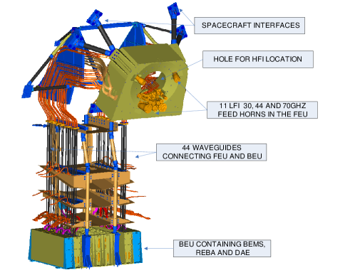
Figure 1: A drawing of the LFI with its spacecraft interfaces.

2.2 The LFI radiometer design

The LFI array is made up of eleven Radiometric Chain Assembly (RCA) (Figure 2) each incorporating the two radiometers connected to the feed horn. Each radiometer includes a pair of amplification/detection chains correlated through a pair of hybrid couplers, constituting a continuous-comparison device Bersanelli et al. (2009). In this scheme, the difference between the inputs to each of the chains (the signal from the telescope and that from a reference blackbody load, respectively) is continuously being taken. This scheme strongly suppresses 1/f noise generated by instabilities in the RF amplifiers, but not in the receiver elements following the second hybrid coupler. To remove this Back End 1/f, it is necessary to modulate the sign of the comparison using solid-state phase-shifters within the correlation section. The differencing receiver improves the stability at a cost of a factor of $\sqrt{2}$ in sensitivity compared with a total power scheme. Any difference between the sky and reference input signals can give rise to 1/f noise, in the LFI receivers this is further reduced by scaling one of the output data streams by a gain modulation factor "r". The blackbody reference itself must remain at a very stable temperature (see Valenziano et al. (2009)).

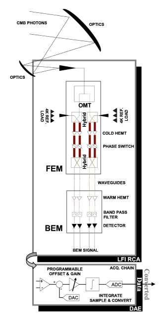
Figure 2: The Low Frequency Instrument Radiometric Chain Assembly (LFI RCA) with the Data Acquisition Electronics diagram.

The intensity $\Delta$T of the smallest detectable signal is given by the radiometer equation (from Skou (1989)):

$$\Delta T=\sqrt{2}\ \frac{T_{\mathrm{in}}+T_{\mathrm{noise}}}{\sqrt{B_{\mathrm{eff}}\cdot\tau}},$$ (1)

where $T_{\mathrm{in}}$ is the input temperature to the radiometer, $T_{\mathrm{noise}}$ is the radiometer noise temperature and $\tau$ is the integration time. Radiometers are characterised by a spectral response g($\nu$) through the radiometer band. The effective bandwidth is defined as:

$$B_{\mathrm{eff}}=\frac{\left[{\int\limits_{0}^{\infty}{g\left(\nu\right)d\nu}}\right]^{2}}{\int\limits_{0}^{\infty}{g^{2}\left(\nu\right)d\nu}}.$$ (2)

3 The analytical LFI Advanced RF model

The need to analyse the effect of LFI non-ideal response and to estimate the impact of systematic effects lead to the development of a radiometer system simulator Battaglia (2002), using the Agilent Advanced Design System (ADS) software. ADS provides Radio Frequency (RF) models for development of system specifications. It contains an RF simulator that predicts performance of complete RF systems and includes a set of block-level RF models for linear and non-linear components. The ADS Design Environment, Data Display, RF System Simulator and Models tools enable the graphic implementation of the receiver components and the possibility to obtain information about the RCA main properties, such as system gain and noise temperature.

3.1 Implementation

The radiometer model is built as a network whose electromagnetic properties can be expressed using scattering parameters, taking into account the losses and reflections of the input signal, when it passes through each network element.

For a generic multi-port network definition, it is assumed that each of the ports is allocated an integer n ranging from 1 to N, where N is the total number of ports. The insertion loss is the loss in load power due to the insertion of a component at some point in a transmission system. In measured insertion loss tables found in literature, the $\left|{S_{21}}\right|^{2}$ is given rather than the pure insertion loss value. In order to evaluate the pure insertion loss, the measured return loss has to be taken into account. The $\left|{S_{21}}\right|^{2}$ is measured experimentally, in decibel, as

$$\left|{S_{21}}\right|^{2}=\frac{{P_{out}}}{{P_{in}}}.$$ (3)

$S_{21}$ includes both the effect of the insertion and the return loss, in fact:

$$S_{21}=10^{\frac{{IL_{dB}}}{{20}}}\sqrt{1-10^{\frac{{RL_{dB}}}{{10}}}},$$ (4)

and the pure insertion loss is given by:

$$IL_{dB}=\;10\;Log_{10}\left({\frac{{\left|{S_{21}}\right|^{2}}}{{1-10^{\frac{{RL_{dB}}}{{10}}}}}}\right).$$ (5)

Return loss, instead, is given by:

$$RL_{dB}=\;10\;Log_{10}\;\left|{S_{11}}\right|^{2},$$ (6)

and total system gain is obtained by:

$$G\left({dB}\right)\ =10\;Log_{10}\left({\frac{{P_{out}}}{{K_{B}\;\Delta\nu\left({T_{noise}+T_{in}}\right)}}}\right),$$ (7)

where $T_{\mathrm{in}}$ is the input load temperature and $P_{\mathrm{out}}$ the corresponding power at detector output; $\Delta\nu$ is the effective bandwidth and $K_{\mathrm{B}}$ is the Boltzmann’s constant. $T_{\mathrm{noise}}$, the system noise temperature is the input load temperature necessary to generate, in a noiseless system, the same output voltage of the noisy device with zero input load.

3.1.1 Devices implementation

Figure 3 shows a schematic of the implementation of the Analytic LARFM. The elements that constitute the RCA receiver shown in Figure 2 have been modelled in ADS starting from n-port device models, amplifiers, hybrids, wave-guides models and equation-based models.

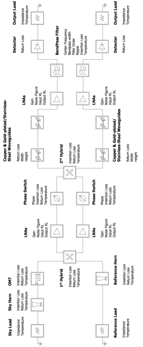
Figure 3: The Analytical LARFM graphical representation in the ADS design environment. Each component is a port device completely characterised by the parameters displayed in the figure.

Input Loads. The receiver input load is generated by the port component termination. It is a $50\Omega$ resistance at temperature $T_{ant}$ that produces a power noise equal to $P=K_{B}T_{ant}\Delta\nu$, where, in order to simulate the power absorbed by the sky and reference feed horns, $T_{ant}$ is the antenna temperature related to the thermodynamic temperature $T$ by:

$$T_{ant}=\frac{\frac{h\nu}{kT}}{e^{\frac{h\nu}{kT}}-1}T.$$ (8)

Feed Horn and OMT. The sky and reference feed horns, as well as the OMT, are modelled as two-port devices, completely characterised by their scattering parameters - expressed in terms of insertion loss and return loss - and by their physical temperature, taking into account the noise temperature $T_{noise}$ generated by the component itself into the network. Given an input signal $T_{in}$ at the input port of, e.g., a feed horn, the signal at the output of the element is given by:

$$T_{out}=\left|S_{21}\right|^{2}T_{in}+T_{noise}.$$ (9)

Hybrids. The hybrid is modelled be a four port S-parameter set of equations using two values of magnitude and phase. They are set to correctly reproduce the in-phase and anti-phase addition of the inputs. The hybrid model by default has a perfect port isolation, but we tested also the effect of a crosstalk between the two paths of the signal (that simulates a non-ideal isolation between the two channels of the radiometer). The hybrid, being a noisy component, is also characterised by the physical temperature of the device.

Front End and Back End Low Noise Amplifiers. The Low Noise Amplifier (LNA) is modelled using the amplifier component of the ADS object library. The LNA model uses scattering parameters for modelling the amplifier gain ($S_{21}$) and reflections at the input and output ports of the device ($S_{11}$ and $S_{22}$); minimum noise figure ($NF_{min}$) at optimum source reflection ($S_{opt}$) and equivalent noise resistance $R_{n}$ are used instead of noise figure to characterise the amplifier noise, providing also a correct return loss modelling response.

Phase Switch. The phase switch model is a two ports system. Scattering parameters are defined in polar coordinates, so that the change in phase is obtained by setting the $S_{21}$ parameter phase to 180 degrees. The temperature parameter characterises the noise properties of the phase switch model, as for the feed horn and OMT models.

Waveguides. The RCA waveguides are modelled into two parts, the copper waveguide model and the gold-plated/stainless-steel waveguide model. Given the high thermal conductivity of copper, the copper waveguide model consists in a single rectangular waveguide element at the same temperature of the Front End Module, i.e. 22K. At the input and output ports two impedance transformers play a double role: they enable the waveguide matching to the characteristic impedance of the network (50 $\Omega$) and they model the waveguide flanges return loss.
The gold-plated and stainless-steel waveguide model, although characterised by the same parameters, is more complex than the copper one, including several rectangular waveguide elements, taking into account the linear temperature gradient between the two flanges.

In fact the stainless steel section interfaces to two heat sinks at either end, one at 300 K and the other at 22 K. The thermal distribution along the stainless steel waveguide is critical due to its high electrical resistivity. So, with reference to Figure 4, the stainless steel section has been modelled so that the temperature at the flanges and shields (V-groove) interfaces is preserved. For the gold plated sections the value for gold resistivity has been used.

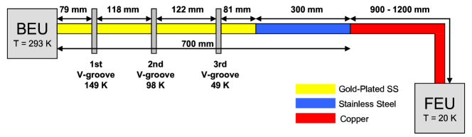
Figure 4: Schematic of the temperature distribution along the waveguides. V-grooves are thermal shields that isolate the cold Front End (22K) from the warm Back End Unit (293K).

By setting the dimensions (width and height) of the waveguides section, the temperatures at the interfaces and the return loss at the flanges, the model is able to reproduce a cryogenic response of the waveguides, in terms of the insertion loss in the simulated frequency band.

Bandpass filter. Its design is a Chebyshev response bandpass filter and its parameters (see Figure 3 for a complete list) completely constrain the insertion loss in the passband and the slope at the cut-off frequency. From the noise temperature analysis point of view, the band pass filter behaves like an attenuator, such as OMT and feed horns.

Detector. The detector has been modelled with a two ports system characterised by a return loss value. The power conversion and integration over the band are performed by an appropriate calculation envelope, available in ADS, so that the output voltage integrated over the frequency band $\Delta\nu$ of the radiometer is given by:

$$V_{out}=\int_{\Delta\nu}G\cdot P_{out}(\nu)~{}d\nu,$$ (10)

where G is a gain factor and $P_{out}(\nu)=V_{out}(\nu)^{2}/R$, being $V_{out}(\nu)$ the simulated output voltage as a function of the frequency and $R$ = 50 $\Omega$ the impedance of the network.

Running ADS simulations it is possible to calculate:

• scattering parameters over the band for the whole RCA model and component by component;

• output voltage over the band;

• integrated output voltage.

3.2 Model verification

The model is verified first at single component level and then at RCA level.

3.2.1 Component level verification

The functional consistency of each radiometer component is verified evaluating scattering parameters, output voltage and noise temperature. At single component level the S-parameters are verified by the ADS primitive models themselves, so that a verification of sub-groups of cascaded elements has been carried out, e.g. cascaded feed horn and OMT. The simulated scattering parameters exactly match with those calculated using the scattering matrix theory, giving confidence that ADS applies the same expressions to compute scattering parameters for a cascaded system.

Given the large quantity of cascaded elements, the validation of the waveguides model is performed by comparing the simulation results with the measured $S_{21}$ at room temperature. Then a prediction of their behaviour at cryogenic temperature is performed using the model, since no cryogenic measurements are available for the waveguides. Figure 5 show a comparison between simulation and measurements for the 30 GHz assembled waveguide (copper section and gold-plated/stainless steel section) at ambient temperature (300K).

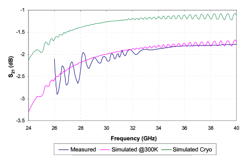
Figure 5: 30 GHz waveguide $S_{21}$ at ambient temperature (measured and simulated) and cryogenic temperature (simulated only). Ripples in measurements are due to reflections within the test set-up; those in simulations are due to the impedance mismatch at the flanges interfaces, since -30 dB return loss is set in this simulation.

Cryogenic simulation shows that the $S_{21}$ is about 1dB better than that measured and simulated at ambient temperature. The cryogenic model takes into account for the copper and gold-plated/stainless steel resistivity dependence on the temperature distribution along the waveguides.

To evaluate the reliability of the model, functional tests and performance tests have been performed. Functional test goals included calibration of the system and a check of the correct mechanism for phase switching.
The calibration factor, $G$, giving the conversion of the diode’s output signal (in volts) into physical units (in kelvins), is defined as:

$$G=\frac{T_{1}-T_{2}}{V_{1}-V_{2}}\equiv\frac{\Delta T}{\Delta V},$$ (11)

where $\Delta$T is the variation between two different input temperatures and $\Delta$V is the corresponding variation in the output voltages. From equation 11 it follows that the calibration factor $G$ is independent of the temperature of the reference load.
The following simulation set-up has been used to calculate the calibration factor:

• Reference load temperature is fixed to 4K;

• Sky load temperature is changed between 20K and 77K;

All Phase Switches conditions have been analysed: both radiometer branches with 0 degree lag; both branches with 180 degree lag; the intermediate status in which only one branch signal is 180 degree shifted (labelled (0, 180) and (180 , 0) in Figure 6). Note that the effect of the lag on a single branch of the radiometer is to reverse the sky and reference signal at the outputs of the radiometer. The simulation has been repeated by fixing the sky load temperature to 4K and varying the reference load between 20K and 77K. Figure 6 shows the calibration factor $G$ in the 30 GHz RCA frequency band, in any status of the two phase switches. Minor differences between the two results are due to asymmetries in the RCA (presence of the OMT in the sky input).

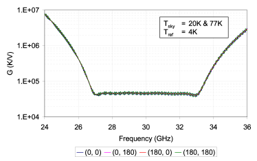
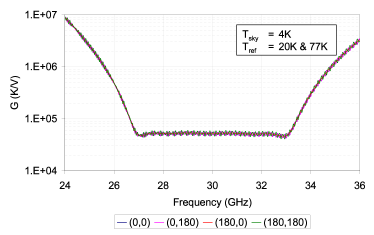
Figure 6: Calibration test results at 30 GHz. The factor $G$ is plotted in K/V versus frequency for fixed sky (left) and reference (right) load temperatures. The calibration factor is independent of phase switch status, labelled as ($Lag_{1}$, $Lag_{2}$).

3.2.2 System level verification

Performance tests have been conducted, including system gain and system noise temperature calculus in the LARFM. All components parameters are set to their nominal value as from the Planck LFI specifications and requirements. The case of an RCA characterised by the insertion loss only is simulated; then simulations are repeated by taking into account for the reflections of the input signal (return loss). (Figure 7) shows a generally good agreement with expected behaviour. Reflections cause a general fall of the system gain value and the formation of band ripples, which contribute to an effective bandwidth reduction. System noise temperature is also affected by the presence of reflections at the waveguides flanges, causing ripples; moreover its mean value in the frequency band increases to about 1.5%.

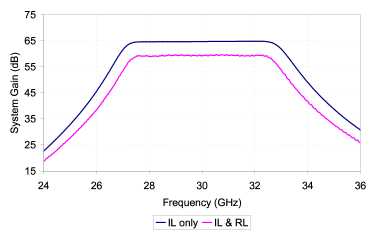
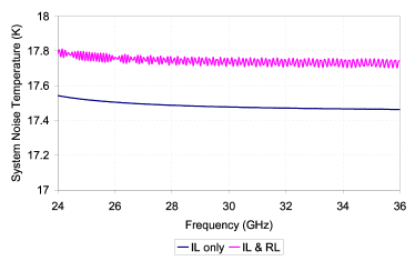
Figure 7: System Total Gain and System Noise Temperature of a 30 GHz RCA characterised by insertion loss only and both insertion loss and return loss. When reflections are calculated by the simulator, the total gain is reduced and the system noise temperature increases.

3.3 Applications

3.3.1 Instrument performances with two FEM prototypes

As a first application of the LARFM to the analysis of the instrument performances Franceschet (2004), we evaluated the system response in the frequency band in two different configurations including two prototypes of the Front End amplifiers at 44 GHz, whose performances, in terms of input/output return loss and total gain are measured in the frequency range 38–50 GHz (Figure 8). The LNA noise figure is given by the measurements on a third LNA and has not changed during the entire analysis of the prototypes; its profile is visible in System Noise Temperature simulation for the nominal case (see Figure 9, right).

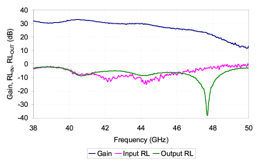
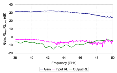
Figure 8: (Left) The first 44 GHz LNA prototype performances: input return loss, output return loss and gain measured at 293K. (Right) The second 44 GHz LNA prototype measurements at 295K.

In order to evaluate the effect of the Front End LNA performance on the system total gain, noise temperature and effective bandwidth, we set all RCA parameters, with the exception of those of the Front End amplifiers, to their nominal value at 44 GHz. The in-band performances of the two LNA prototypes are measured at ambient temperature (a worst case). The nominal case, with the LNA input return loss $RL_{in}$ = -5 dB, output return loss $RL_{out}$ = -6 dB and gain $G$ = 30 dB, is also simulated for a comparison.

Figure 9 shows that in both simulations including LNA prototypes, the total gain follows the shape of the corresponding prototype, with wide ripples for frequencies above 47 GHz, due to the effect of the input return loss. As expected, the RCA with the second LNA prototype exhibits better performance in terms of total system gain, in particular for frequencies above 44 GHz. Simulations show similar results for the system noise temperature: it rapidly diverges for frequencies above 48 GHz in the first prototype simulation; the input return loss of the LNA plays a leading role in this simulation, since nearly all incoming power is reflected at the LNA input port.

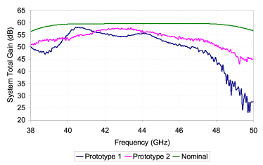
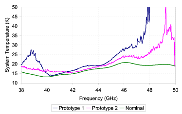
Figure 9: System Total Gain and Noise Temperature simulated for 44 GHz RCA’s including two LNA prototypes and the nominal case (LNA performances as from requirements).

The effective bandwidth, as calculated by the LARFM for all test cases is summarized in Table 1.

Frequency Range	38–50 GHz	39.6–48.4 GHz
$B_{eff}$ Prototype 1	6.93	6.28
$B_{eff}$ Prototype 2	8.94	7.45
$B_{eff}$ Nominal	11.75	8.84

Table 1: Effective bandwidth $B_{eff}$ in the measured data frequency range (38–50 GHz) and in the Planck LFI required frequency bandwidth (20% of the centre frequency).

This analysis shows that the LARFM is a useful tool to investigate the behaviour of the Planck LFI instrument when in band non idealities characterise the system components.

3.3.2 Effects of OMT asymmetry

If the OMT arms have different performance, in terms of loss and reflection in the frequency band, the two orthogonal components of the polar signal are affected differently, and will be confused with a real polarisation signal when processing the polarisation information. As an application of the LARFM, the impact of asymmetries, in terms of losses and reflections, in each one of the OMT arms on the in-band total system gain is studied. Simulations are performed by setting all RCA parameters to their nominal values, with the exception of the OMT insertion loss and return loss, measured on the Qualification Model (QM) of the 30 GHz OMT.

Simulation results in Figure 10 shows that the maximum gain mismatch between the arms of the radiometer is about 0.25% at 30 GHz.

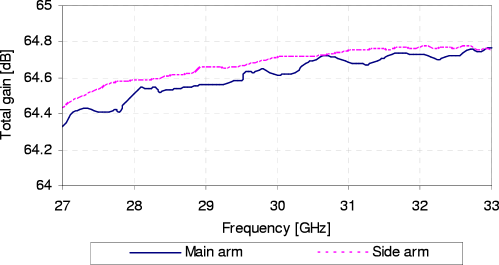
Figure 10: Effect of the OMT in band asymmetries on the total system gain of the 30 GHz RCA Qualification Model.

For a description of the impact of asymmetries between the two arms of the 30 GHz RCA on the CMB polarisation measurement, the following expression has to be evaluated:

$$\begin{array}[]{l}\Delta\left({\Delta T}\right)=\frac{1}{{\Delta\nu}}\left[{\int{G_{1}\left(\nu\right)T_{sky}\left(\nu\right)d\nu}-\int{G_{1}\left(\nu\right)r_{1}T_{ref}\left(\nu\right)d\nu}}\right]+\\ \quad\quad\quad-\frac{1}{{\Delta\nu}}\left[{\int{G_{2}\left(\nu\right)T_{sky}\left(\nu\right)d\nu}-\int{G_{2}\left(\nu\right)r_{2}T_{ref}\left(\nu\right)d\nu}}\right]\\ \end{array}$$ (12)

where $G_{1}(\nu)$ and $G_{2}(\nu)$ are the gain relevant to the two arms of the radiometer (Figure 10), $T_{sky}$ and $T_{ref}$ are the observed sky temperature and the reference load temperature and $r_{1}$ and $r_{2}$ are the gain modulation factors for both arms of the RCA. The sky signal is parametrised assuming a power-low behaviour for the sky temperature,

$$T_{sky}=\alpha\nu^{-\beta}$$ (13)

where $\alpha$ and $\beta$ are derived from WMAP foreground maps at 23, 33, 41, 61 and 94 GHz and the CMB signal expression,

$$T_{CMB}\left(\nu\right)=\frac{{{{h\nu}\mathord{\left/{\vphantom{{h\nu}{K_{B}T_{0}}}}\right.\kern-1.2pt}{K_{B}T_{0}}}}}{{e^{{{h\nu}\mathord{\left/{\vphantom{{h\nu}{K_{B}T_{0}}}}\right.\kern-1.2pt}{K_{B}T_{0}}}}-1}}T_{0}$$ (14)

where $T_{0}$ = 2.725 K, and $K_{B}$ is the Boltzmann’s constant. The K, Ka and Q band data fix the $\alpha$ and $\beta$ values in the ranges $\alpha\in[5\cdot 10^{3},6\cdot 10^{3}]$ and $\beta\in[0.25,0.35]$. The reference load temperature follows the frequency dependant 4.8K black-body curve for this analysis.
By calculating the integrals for the specified variation ranges of the normalisation parameter $\alpha$ and of the spectral index $\beta$, the difference between the two differenced output signals, i.e. the expression $\Delta(\Delta T)$, is plotted in Figure 11.

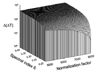
Figure 11: Difference, in mK, between the final output of the two branches of the radiometer.

4 The Real-Data LFI Advanced RF Model

During the qualification and performance tests, each component of the LFI radiometers was independently characterised in terms of frequency response. These hardware measurements replaced the parameters used in the analytical version of the LARFM with the objective of estimating the effective response of the 44 channels of the LFI flight hardware.

The new LARFM maintains the same implementation just for the waveguides simulator, while the other units are replaced by their measurements. Moreover, the main objective of the LARFM became the estimation of the bandpass response, see Zonca et al. (2009), due to the high impact of systematic effects on end-to-end bandpass measurements. The next sections explain the implementation and the results obtained with the LARFM.

4.1 Implementation

Figure 12 shows a schematic of the implementation of the Real-Data LARFM. In this model the pseudo-correlation strategy is not considered, see section 4.1.2, so each channel is completely independent from the other channel of the same radiometer. Moreover, the number of devices is strongly reduced because FEM and BEM devices where fully characterized after assembly.

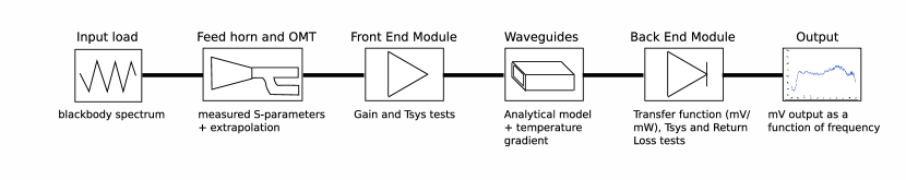
Figure 12: Model schematic for each LFI channel: feed horn and OMT are characterized by their S-parameters; FEM by gain and noise temperature; waveguides are simulated analytically; BEM by return loss, transfer function and integrated noise temperature.

4.1.1 Feed horn and OMT

Feed horn and OMT return losses were measured on their assembly, injecting the test signal from the OMT port to be connected to the FEM. Insertion losses, instead, are available for the OMT only, but the impact of the feed horn is negligible. Feed horn and OMT model is a single Sparameters passive component based on these data.

4.1.2 FEM

A FEM model considering the pseudo correlation strategy needs spectral response measurements of each component assembling the FEM:

• Hybrids

• Low Noise Amplifiers

• Phase switches

• Internal FEM waveguides

However, all these components when tightly assembled into the FEM change their response significantly due to mutual interactions. It is therefore more reliable to use the data from the tests of the complete FEM.

Each channel is simulated independently from the others using data from gain and noise temperature tests performed by the FEM producers. Each channel is considered as a total power radiometer frozen in the configuration of the phase switches states which connects it to the sky signal. Indeed, there are two phase switch state combinations where the same BEM channel is connected to the sky arm, but, after phase switch balancing, the responses match better than $\sim.1dB$.

In ADS, the FEM has been modelled as an amplifier with gain given by the performance tests on each FEM channel and noise figure computed by the system temperature as:

$$F=10\log_{10}\left({\frac{{T_{sys}}}{{290K+1}}}\right).$$ (15)

FEM $S_{11}$ could only be measured at ambient temperature, therefore the LARFM implements the mean expected value $S_{11}=-7dB$. The RCA is then studied in an ideal configuration, in which all four RCA channels are looking simultaneously to the sky signal.

4.1.3 BEM

The BEM model is made up of:

• Reflection only Sparameter component for return loss

• A noise generator for the noise temperature

• An equation object for the gain

In order to model the whole RCA, the RF signal coming from the FEM through the waveguides is summed with a noise generator based on the measured BEM noise temperature. This signal is then amplified by the measured spectral transfer function converting input power to output volts at a given frequency, which includes the effect of all the BEM components together.

The output is a bandpass response of the complete RCA which can then be integrated over frequency in order to compute the detector voltage output that can be compared with test results.

During the flight hardware test campaign, 30 and 44 GHz RCAs showed signal compression at BEM level, i.e. the BEM output doesn’t increase linearly with the input temperature. This effect has a big impact on system temperature calculation, because the data extrapolation process emphasises even a small non-linearity. Therefore, a parametric non linear analytic model was developed in Mennella et al. (2009b) in order to fit test data for extracting the overall RCA gain, system temperature and BEM compression factor. The model is based on the following equation:

$$V_{out}=G_{0}\cdot\left[{\frac{1}{{1+b\cdot G_{0}\cdot\left({T_{A}+T_{noise}}\right)}}}\right]\cdot\left({T_{A}+T_{noise}}\right),$$ (16)

where $T_{A}$ is the antenna temperature, $G_{0}$ is the linear gain and $b$ is the compression factor. The compression factor is a single scalar value per channel which represents the BEM gain dependence on the input power. BEM tests were performed at a power level where compression is expected. The first operation to perform then is to calculate the linear gain by using the known information on the compression factor measure in the relevant tests. The equation used is:

$$G_{lin}=\frac{{G_{test}}}{{1-b\cdot P_{in}\cdot G_{test}}},$$ (17)

where $G_{test}$ is the total BEM gain or transfer function (i.e. output voltage vs input power), $b$ is the scalar compression factor, $P_{in}$ is the input power for the BEM test and $G_{lin}$ is the computed linear gain. The last step is to substitute $G_{lin}$ for the gain parameter of the BEM and change the equation describing the BEM to:

$$V_{out}=\frac{{G\cdot P_{in}}}{{\left({1+b\cdot P_{in}\cdot G}\right)}}.$$ (18)

4.2 Results

The Real-Data LARFM outputs are the channel bandpasses, volt outputs, gains and noise temperatures either on the full RCA or in any section of it. These data are the basis of several analyses on the LFI radiometers, in the following paragraphs we are going to introduce the most interesting.

The most important result of the LARFM is bandpass estimation, see Zonca et al. (2009). Figure 13 shows a good agreement between LARFM bandpasses and end-to-end measurements, the end-to-end measurements are however affected by systematic effects and their quality is not sufficient for a quantitative analysis.

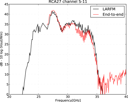
Figure 13: LFI27S-11 at 30 GHz. Comparison of LARFM bandpasses with end-to-end swept source measurements performed on WR28 nominal bandpass, between 26.5 and 40 GHz, see Zonca et al. (2009).

Figure 14 shows the output voltage as a function of input load temperature measured in a linearity test compared to the LARFM results assuming a linear BEM response and implementing the BEM non-linear model as explained in section 4.1.3. The compression parameter $b$ of Eq. 18 was measured using the test results and the comparison shows a good agreement between the non-linear model and the measurements.

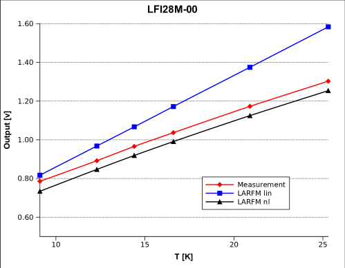
Figure 14: Output voltage versus temperature for a linearity test compared to the LARFM linear and non-linear BEM models.

The LARFM was also successfully applied to predict the impact on bandpasses of the substitution of a damaged FEM unit with a spare unit, to assess whether it would be acceptable to replace or necessary to repair the unit. Figure 15 shows the impact on the LARFM bandpasses of the eventual substitution of the flight FEM with the spare unit on RCA 24. The response of the spare FEM is more structured than the nominal unit and the bandwidth is reduced by about $20\%$ (see Zonca (2009)), the unit was successfully repaired.

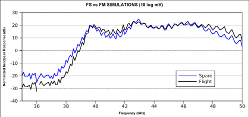
Figure 15: Comparison between LARFM bandpasses with nominal versus spare FEM on LFI24M-00

The RF model has been used also during the cryogenic test campaign to successfully investigate the saturation at the BEM diode, by modelling the RF power level at the diode input.

A more direct use of the model is foreseen in the unfortunate case of the radiometers working in non-nominal configurations, for example different thermal conditions. In this case it is possible to estimate the impact of these non-nominal conditions on each component and then make use of the LARFM to simulate the non-nominal behaviour in terms of bandpasses and output voltage.

5 Conclusions

We have described the LFI Advanced RF Model, based on commercial software tools and measurements of the radiometer component at single unit level. The LARFM provides a good description of the response of each of the 44 channels of the Planck-LFI array, such as radiometer response (including non-linear behaviour), system gain, noise temperature, spectral shape of the radiometers bands.

The measurements of the scattering parameters of the single units (i.e., feed horns, OrthoMode transducers, front-end modules, waveguides, back-end modules) are very precise (typically better than 0.1dB), while in some cases the end-to-end measurements of the integrated radiometer properties are more difficult. This is the case, for example, for the evaluation of the shape of the spectral bands, whose knowledge is particularly important for polarisation analysis. In these cases, the availability of the LARFM has proved particularly useful.

After being successfully used to support the Planck-LFI design and ground-test campaigns, the model is now incorporated in the LFI data processing centre to allow detailed studies of radiometer behaviour during the Planck survey. Similarly, future precision radiometric instruments will likely require similar models to be developed to support instrument development and data analysis. Our experience has shown the usefulness of such an RF software model and indicates a strategy and some technical tools that may be useful for other projects in the future.

References

- Battaglia [2002] P. Battaglia. Advanced software model of the planck low frequency instrument radiometer. Master’s thesis, Universita’ degli Studi di Milano, 2002.
- Bersanelli et al. [2009] M. Bersanelli et al. Planck pre-launch status: Design and description of the Low Frequency Instrument. A&A, accepted, 2009.
- Franceschet [2004] C. Franceschet. Application of the planck-lfi advanced simulator to performances assessments of the qualification models. Master’s thesis, Universita’ degli Studi di Milano, 2004.
- Lamarre et al. [2009] J.-M. Lamarre et al. Planck pre-launch status: the HFI instrument, from specification to actual performance. A&A, submitted, 2009.
- Mennella et al. [2009a] A. Mennella et al. Planck pre-launch status: Low Frequency Instrument calibration and scientific performance. A&A, accepted, 2009a.
- Mennella et al. [2009b] A. Mennella et al. The linearity response of the Planck-LFI flight model receivers. JINST, 4(12):T12011, 2009b. 10.1088/1748-0221/4/12/T12011. URL http:/stacks.iop.org/1748-0221/4/T12011.
- Skou [1989] N. Skou. Microwave Radiometer Systems: Design and Analysis. Artech House Inc., 1989.
- Tauber et al. [2009] J.A. Tauber et al. Planck pre-launch status: The Planck mission. A&A, submitted, 2009.
- Valenziano et al. [2009] L. Valenziano et al. Planck-LFI: Design and Performance of the 4 Kelvin Reference Load Unit. JINST, 4(12):T12006, 2009. 10.1088/1748-0221/4/12/T12006. URL http:/stacks.iop.org/1748-0221/4/T12006.
- Villa et al. [2009] F. Villa et al. Planck pre-launch status: calibration of LFI flight model radiometers. A&A, submitted, 2009.
- Zonca [2009] A. Zonca. Advanced modelling and combined data analysis of Planck focal plane instruments. PhD thesis, Universita’ degli Studi di Milano, 2009.
- Zonca et al. [2009] A. Zonca et al. Planck-LFI radiometers’ spectral response. JINST, 4(12):T12010, 2009. 10.1088/1748-0221/4/12/T12010. URL http:/stacks.iop.org/1748-0221/4/T12010.