The topology of Helmholtz domains

Abstract.

The goal of this paper is to describe and clarify as much as possible the 3–dimensional topology underlying the Helmholtz cuts method, which occurs in a wide theoretic and applied literature about Electromagnetism, Fluid dynamics and Elasticity on domains of the ordinary space ${\mathbb{R}}^{3}$. We consider two classes of bounded domains that satisfy mild boundary conditions and that become “simple” after a finite number of disjoint cuts along properly embedded surfaces. For the first class (Helmholtz), “simple” means that every curl–free smooth vector field admits a potential. For the second (weakly–Helmholtz), we only require that a potential exists for the restriction of every curl–free smooth vector field defined on the whole initial domain. By means of classical and rather elementary facts of 3–dimensional geometric and algebraic topology, we give an exhaustive description of Helmholtz domains, realizing that their topology is forced to be quite elementary (in particular, Helmholtz domains with connected boundary are just possibly knotted handlebodies, and the complement of any non–trivial link is not Helmholtz). The discussion about weakly–Helmholtz domains is a bit more advanced, and their classification appears to be a quite difficult issue. Nevertheless, we provide several interesting characterizations of them and, in particular, we point out that the class of links with weakly–Helmholtz complements eventually coincides with the class of the so–called homology boundary links, that have been widely studied in Knot Theory.

1. Introduction

Hodge decomposition is an important analytic structure occurring in a wide theoretic and applied literature on Electromagnetism, Fluid dynamics and Elasticity on domains of the ordinary space ${\mathbb{R}}^{3}$ (see a selection of titles in “Section A” of our References). In [6], one can find a friendly introduction to this topic. Helmholtz’s “cuts method” arised in this framework, as far as we understand, in order to obtain a more effective description of the Hodge decomposition of the space of $L^{2}$–vector fields on a given domain, which could also allow explicit numerical processings. These ideas can be incorporated in the notion of so–called Helmholtz domain. Roughly speaking, a Helmholtz domain is a bounded domain that becomes “simple” after a finite number of cuts along disjoint surfaces. It turns out that there is a bit of indeterminacy in the literature about the right meaning of “simple”. Requiring the domain to be simply connected certainly suffices. However, the (possibly weaker) condition consisting in the existence of potentials for curl–free smooth vector fields sounds more pertinent to the actual setting. Apparently, the relationship between such a priori different notions is not widely well established. In Section 16 of [6], one can find a historical account about the way embryonic forms of homotopy and homology groups of spatial domains had been introduced by Helmholtz, Thomson and reconsidered by Maxwell in the study of Electro and Fluid dynamics. Quoting from page 439:

“Thomson introduced an embryonic version of the one–dimensional homology $H_{1}(\Omega)$ in which one countes the number of “irreconcilable” closed paths inside the domain $\Omega$. This was subject to the standard confusion of the time between homology and homotopy of paths: homology was the appropriate notion in this setting, but the definitions were those of homotopy”.

One could say that such a confusion of the early times somehow propagated by internal paths till the present days (including true misunderstandings, see the discussion of Example 3.3 below).

On the other hand, spatial domains (whose study includes, for example, Knot Theory) represent a non–trivial specialization of 3–dimensional manifolds and, since Poincaré’s Analysis Situs (1895) ([36] provides an useful historical account), an important range of applications of the ideas and techniques of (3–dimensional) Geometric and Algebraic Topology developed time by time.

The first aim of the present largely expository paper is to completely clarify the topology of Helmholtz domains, just by applying a few classical results or rather elementary facts of 3–dimensional topology.

The first results we recognize (see Theorem 3.1, Corollary 3.2) show that, under mild assumptions on the boundary (e.g. when the boundary is locally Lipschitz, condition which is usually taken for granted in the literature on Helmholtz domains), the notions of “simplicity” mentioned above are indeed equivalent to each other. Moreover, it turns out that simple domains admit a clear and easy description: they are just the complement of a finite number of disjoint balls in a larger ball. In the case of polyhedral boundaries, this is due to Borsuk [23] (1934). The validity for more general (locally flat) topological boundaries depends on later deep results that we will recall in Theorem 2.8. The proof we will provide is based on elementary properties of the Euler–Poincaré characteristic of compact surfaces and 3–manifolds and (like in [23]) eventually reduces to the celebrated Alexander Theorem [20] (1924) asserting that every polyhedral (locally flat indeed) 2–sphere in ${\mathbb{R}}^{3}$ bounds a 3–ball. In [34] (1948), Fox obtained Borsuk’s Theorem as a corollary of his reimbedding theorem (see Section 4.1 below). However, Fox’s arguments are admittedly inspired by Alexander’s results and techniques.

Once simple domains have been completely described, it is rather easy to give an exhaustive characterization of general Helmholtz domains (see Theorem 4.5). In a sense, this is a disappointing result, as it shows that the topology of Helmholtz domains is forced to be quite elementary. For example, Helmholtz domains with connected boundary are just (possibly knotted) handlebodies, and the complement of any non–trivial link is not Helmholtz.

In Section 5, we introduce and discuss the strictly larger class of so–called weakly–Helmholtz domains. Roughly speaking, such a domain can be cut along a finite number of disjoint surfaces into subdomains on which curl–free smooth vector fields, that are defined on the whole original domain, admit potentials. We believe that this requirement naturally weakens the Helmholtz condition, thus allowing to apply the method of cuts to topologically richer classes of domains. Unlike in the case of Helmholtz domains, we are not able to give an exhaustive classification of weakly–Helmholtz ones. However, we will provide several interesting characterizations of weakly–Helmholtz domains. In particular and remarkably, we realize that the class of links with weakly–Helmholtz complements eventually coincides with the class of so–called homology boundary links. In particular, every knot and every classical boundary link has weakly–Helmholtz complement. Homology boundary links are very widely studied in Knot Theory, and it is a nice occurrence that the Helmholtz cut method leads to such a distinguished class of links.

Paper [11] is a sort of complement to the present one. It deals with an effective description of the Hodge decomposition of the space of $L^{2}$–vector fields on any bounded domain of ${\mathbb{R}}^{3}$ with sufficiently regular boundary, without making use of any cuts–type method.

We stress that, from the strict 3–dimensional topology viewpoint, the results of this paper are largely applications of classical and well–known facts of Differential/Algebraic/Geometric Topology, that are usually covered by basic courses on these subjects. This reflects upon “Section B” of our References, that contains well established books on these subjects, that are exhaustive for our needs. In order to make the exposition simpler for a reader not too familiar with such topics, instead of recalling these facts in one comprehensive section, we have preferred to do it time by time. As already said, the discussion about Helmholtz domains only needs simple facts about the Euler–Poincaré characteristic (see Section 3.3), together with Alexander’s Theorem. Very clear and accessible proofs of this last result are available (e.g. in [44]). The discussion about weakly–Helmholtz domains is a bit more advanced. More information on the algebraic topology of spatial domains is developed in Section 5.1, and we will make intensive use of duality.

On the other hand, we hope that this paper could be of some utility to people interested in research areas mentioned at the beginning of this introduction. The rôle of the (algebraic) topology of domains had already been stressed in [6] and [12] (for example in order to justify the dimension of the Hodge decomposition summands). Hopefully, the present work should integrate the papers just mentioned, by unfolding the 3–dimensional topology underlying the Helmholtz cuts method.

Aknowledgements. The first two authors like to thank R. Ghiloni for having “discovered” the Helmholtz domains literature, and involved them in the task of clarifying their topology. The third author thanks especially Alberto Valli, for having introduced him to these themes, and convinced him of the utility of such a task. He also thanks Ana Alonso Rodríguez, Annaliese Defranceschi, Domenico Luminati, and Valter Moretti for helpful conversations.

2. Domains

In what follows, smooth maps (whence, in particular, diffeomophisms) or manifolds will always assumed to be of class $C^{\infty}$.

First a few terminology. The terms “disk” and “ball” are often used indifferently, by specifying time by time if they are open or closed. We prefer here to profit of both terms by stipulating that a disk is closed and a ball is the open interior of a disk. More precisely, let $(x_{1},x_{2},x_{3})$ be the usual coordinates of ${\mathbb{R}}^{3}$ and let $D^{3}$ be the standard $3$–disk $\{(x_{1},x_{2},x_{3})\in{\mathbb{R}}^{3}\,|\,x_{1}^{2}+x_{2}^{2}+x_{3}^{2}\leq 1\}$ of ${\mathbb{R}}^{3}$. Identify ${\mathbb{R}}^{2}$ with the plane $x_{3}=0$ of ${\mathbb{R}}^{3}$ and denote by $D^{2}$ the standard $2$–disk defined by $D^{2}:=D^{3}\cap{\mathbb{R}}^{2}$.

Definition 2.1.

A subset $X$ of a manifold $M$ homeomorphic to ${\mathbb{R}}^{3}$ is a $($topological$)$ $3$–disk if, up to homeomorphism, the pair $(M,X)$ is equivalent to $({\mathbb{R}}^{3},D^{3})$, i.e. there exists a homeomorphism $\psi:M\longrightarrow{\mathbb{R}}^{3}$ such that $\psi(X)=D^{3}$. A $($topological$)$ $3$–ball of $M$ is the internal part of a $3$–disk. We say that a subset $Y$ of $M$ is a $($topological$)$ $2$–disk if, up to homeomorphism, the pair $(M,Y)$ is equivalent to $({\mathbb{R}}^{3},D^{2})$. Smooth disks or balls in a smooth $M$ diffeomorphic to ${\mathbb{R}}^{3}$ are defined in the same way by replacing “homeomorphism” with “diffeomorphism”. Disks and balls in an arbitrary 3–manifold $W$ are contained, by definition, in some chart $M$ homeo(diffeo)morphic to ${\mathbb{R}}^{3}$.

By a domain $\Omega$ in ${\mathbb{R}}^{3}$, we will mean a non–empty connected open set, which coincides with the interior of its closure in ${\mathbb{R}}^{3}$, i.e. ${\rm Int}\ \overline{\Omega}=\Omega$. Moreover, throughout the whole paper, domains will always assumed to be bounded, whence with compact closure.

Sometimes it is convenient to identify ${\mathbb{R}}^{3}$ with an open subset of the 3–sphere $S^{3}={\mathbb{R}}^{3}\cup\{\infty\}$ via the stereographic projection from the point “at infinity”. An open subset $\Omega\subset S^{3}$ is a domain if ${\rm Int}\ \overline{\Omega}=\Omega$. Of course every domain in $S^{3}$ has compact closure, and the stereographic projection induces a bijection between domains in ${\mathbb{R}}^{3}$ and domains in $S^{3}$ whose closure does not contain the added point $\infty$.

We denote by $\partial\Omega$ the usual (topological) boundary of $\Omega$, i.e. the set

$$\partial\Omega=\overline{\Omega}\setminus\Omega\,.$$

It turns out (see e.g. Remark 3.5) that domains with “wild” boundary can display pathological behaviours that we would like to exclude from our investigation. We will therefore concentrate our attention on domains with “tame” boundary, carefully specifying what “tame” means in our context.

2.1. Smooth surfaces.

We begin by defining the tamest class of domains one could consider. A smooth surface $S$ in ${\mathbb{R}}^{3}$ is a compact and connected subset of ${\mathbb{R}}^{3}$ such that the following condition holds: for every point $p\in S$, there exist a neighbourhood $U_{p}$ of $p$ in ${\mathbb{R}}^{3}$ and a diffeomorphism $\varphi:U_{p}\longrightarrow{\mathbb{R}}^{3}$ such that $\varphi(U_{p}\cap S)=P$, where $P$ is an affine plane. In other words, $S\subset{\mathbb{R}}^{3}$ is a smooth surface if the pair $({\mathbb{R}}^{3},S)$ is locally modeled, up to diffeomorphism, on the pair $({\mathbb{R}}^{3},{\mathbb{R}}^{2})$. For any system $(x_{1},x_{2},x_{3})$ of linear coordinates on ${\mathbb{R}}^{3}$, for $i=1,2,3$, set $H_{i}:=\{(x_{1},x_{2},x_{3})\in{\mathbb{R}}^{3}\,|\,x_{i}=0\}$. By the Inverse Function Theorem, $S$ is a smooth surface if and only if it is locally the graph of a real smooth function (defined on an open subset of some $H_{i}$).

Proposition 2.2.

Every smooth surface $S$ in ${\mathbb{R}}^{3}$ disconnects $S^{3}$ in two domains $\Omega(S)$ and $\Omega^{*}(S)$.

Let us sketch a proof of Proposition 2.2 that uses classical tools from Differential Topology (exhaustive references for our needs are, for instance, [56] and [46]). By the very definition of surface, if $p$ is a point of $S$, then $S$ disconnects small neighbourhoods of $p$ into two connected components. Together with the fact that $S$ is connected, this readily implies that $S^{3}\setminus S$ consists of at most two connected components. Suppose now, by contradiction, that $S^{3}\setminus S$ is connected. Then any closed interval transverse to $P$ in a local model can be completed in $S^{3}\setminus S$ to an embedded smooth circle $f_{0}:S^{1}\longrightarrow C_{0}\subset S^{3}$ that transversely intersects $S$ in exactly one point. Since $S^{3}$ is simply connected (see Subsection 2.6 for a brief discussion of such a notion), $f_{0}$ is smoothly homotopic to an embedded circle $f_{1}:S^{1}\longrightarrow C_{1}\subset S^{3}$ that does not intersect $S$. Moreover, we can assume that there exists a smooth homotopy $F:S^{1}\times[0,1]\longrightarrow S^{3}$ between $f_{0}$ and $f_{1}$, which is transverse to $S$. Then the set $F^{-1}(S)$ consists of a finite disjoint union of smooth circles or closed intervals having $F^{-1}(S)\cap(S^{1}\times\{0,1\})$ as set of end–points. In particular, $F^{-1}(S)\cap(S^{1}\times\{0,1\})$ should be given by an even number of points, while we know that it consists of just one point. This gives the desired contradiction.

Notation. From now on, whenever $S\subset{\mathbb{R}}^{3}\subset S^{3}$ is a smooth surface, we will denote by $\Omega(S)$ and $\Omega^{\ast}(S)$ the connected components of $S^{3}\setminus S$. We will also assume that $\infty\in\Omega^{\ast}(S)$, so $\Omega(S)$ is the unique bounded component of ${\mathbb{R}}^{3}\setminus S$, while $\Omega^{\prime}(S):=\Omega^{*}(S)\setminus\{\infty\}$ is the unique unbounded component of ${\mathbb{R}}^{3}\setminus S$. In particular, $\Omega(S)$ is a domain in ${\mathbb{R}}^{3}$ and $\partial\Omega(S)=S$. The local model of $(\Omega(S),S)$ at every boundary point is given by $(P_{+},P)$ where $P$ is an affine hyperplane as above, and $P_{+}\subset{\mathbb{R}}^{3}$ is a half–space bounded by $P$.

Definition 2.3.

A domain $\Omega$ in ${\mathbb{R}}^{3}$ has smooth boundary if $\partial\Omega$ consists of the disjoint union of a finite number of smooth surfaces.

It readily follows from the definitions that the closure of a domain with smooth boundary admits a natural structure of compact smooth manifold with boundary.

The following lemma is an immediate consequence of the previous discussion.

Lemma 2.4.

Let $\Omega$ be a domain with smooth boundary. Then we can order the boundary surfaces $S_{0},S_{1},\dots,S_{h}$ in such a way that:

1. The $\overline{\Omega(S_{j})}$’s, $j=1,\ldots,h$, are contained in $\Omega(S_{0})$ and are pairwise disjoint.

2. $\Omega$ is given by the following intersection:

   $$\Omega=\Omega(S_{0})\cap\bigcap_{j=1}^{h}\Omega^{*}(S_{j})\,.$$

2.2. Orientation and tubular neighbourhoods

Let $S\subset{\mathbb{R}}^{3}$ be a smooth surface. We claim that $S$ is orientable. In fact, if ${\mathbb{R}}^{3}$ is oriented by means of the equivalence class of its standard basis $(e_{1},e_{2},e_{3})$, then $S$ can be oriented as the boundary of $\Omega(S)$, via the rule “first the outgoing normal vector”. More explicitly, for each $p\in S$, one can consistently declare that a basis $(v_{1},v_{2})$ of the tangent space $T_{p}S$ of $S$ at $p$ is positively oriented if and only if $(n,v_{1},v_{2})$ is a positively oriented basis of ${\mathbb{R}}^{3}$, where $n$ is a vector orthogonal to $T_{p}S$ and pointing outward $\Omega(S)$.

For every $\epsilon>0$, let us define the $\epsilon$–neighbourhood $N_{\epsilon}(S)$ of $S$ in ${\mathbb{R}}^{3}$ by setting

$$N_{\epsilon}(S):=\{x\in{\mathbb{R}}^{3}\ |\ {\rm dist}(x,S)\leq\epsilon\}\,.$$

If $\epsilon$ is small enough, then the pair $(N_{\epsilon}(S),S)$ is diffeomorphic to $(S\times[-1,1],S\times\{0\})$. If $r:N_{\epsilon}(S)\longrightarrow S$ is the natural retraction such that $r(x)$ is the nearest point to $x$ (such a retraction is well–defined provided that $\epsilon$ is sufficiently small), then, for every $x\in S$, the set $r^{-1}(x)$ is a straight copy of $[-\epsilon,\epsilon]$. Moreover, $N_{\epsilon}(S)\cap\overline{\Omega(S)}$ is mapped onto $S\times[-1,0]$, hence it is a collar of $S$ in $\overline{\Omega(S)}$. Similarly for $N_{\epsilon}(S)\cap\overline{\Omega^{\prime}(S)}$. If $C$ is a smoothly embedded circle in ${\mathbb{R}}^{3}$ and $\epsilon$ is small enough, then $N_{\epsilon}(C)$ also is a tubular neighbourhood of $C$, diffeomorphic to a (closed) solid torus $D^{2}\times S^{1}$ and having $C$ as core.

2.3. Link complements.

A link $L=C_{0}\cup\ \dots\cup C_{h}$ in $S^{3}$ is the union of a finite family of smoothly embedded disjoint circles $C_{j}$. If $h=0$, then $L$ is called a knot. Suppose that $\infty\in C_{0}$, hence $A(L)=S^{3}\setminus L$ is a connected open set in ${\mathbb{R}}^{3}$. With our definitions, since $\overline{A(L)}={\mathbb{R}}^{3}$, the internal part of $\overline{A(L)}$ does not coincide with $A(L)$ and $A(L)$ is not a domain. However, to $L$ there is associated the domain $\mathsf{C}(L)=S^{3}\setminus U(L)$, where $U(L)$ is the union of small disjoint closed tubular neighbourhoods of the $C_{j}$’s. We call $\mathsf{C}(L)$ complement–domain of $L$. The boundary component of $\mathsf{C}(L)$ corresponding to $C_{j}$ is a smooth torus $T_{j}$ and, with the above notations, $\Omega^{*}(T_{0})$ and $\Omega(T_{j})$, $j=1,\dots,h$, are open solid tori. It is clear that $\mathsf{C}(L)$ is homotopically equivalent to $A(L)$ (see e.g. [43] for the definition of homotopy equivalence), hence $\mathsf{C}(L)$ and $A(L)$ share all the homotopy type invariants (like the fundamental group). A knot $C=C_{0}$ is unknotted if also $\Omega(T_{0})$ is a solid torus or, equivalently, if $C$ bounds a 2–disk of $S^{3}$. A link has geometrically unlinked components if its components are contained in pairwise disjoint 3–disks of $S^{3}$. A link is trivial if it has geometrically unlinked unknotted components.

Suppose now that $\infty\not\in L$, i.e. consider $L$ as a link of ${\mathbb{R}}^{3}$. We use the symbol $U(L)$ again to indicate the union of small disjoint closed tubular neighbourhoods of the $C_{j}$’s in ${\mathbb{R}}^{3}$. Choose a smooth $3$–ball $B$ of ${\mathbb{R}}^{3}$ containing $U(L)$ and define $\mathsf{B}(L):=B\setminus U(L)$. We call $\mathsf{B}(L)$ box–domain of $L$. Any rigid motion of $S^{3}$ that takes $L$ onto a link $L^{\prime}$ containing the point at infinity establishes a diffeomorphism between the box–domain $\mathsf{B}(L)$ and the complement–domain $\mathsf{C}(L^{\prime})$ with a $3$–disk removed.

The reader observes that the complement– and the box–domains of a link are well–defined, up to diffeomorphism (up to ambient isotopy indeed).

2.4. Cutting along surfaces.

Let $\Omega$ be a domain with smooth boundary. A properly embedded surface $\Sigma$ in $(\overline{\Omega},\partial\Omega)$ is a compact and connected subset of $\overline{\Omega}$ such that:

1. On $\Sigma\setminus\partial\Omega$, $\Sigma$ has the same local model of a smooth surface.

2. If $\Sigma\cap\partial\Omega\neq\emptyset$, then at every point of this intersection, up to local diffeomorphism, the triple $(\overline{\Omega},\partial\Omega,\Sigma)$ is equivalent to the local model $(P_{+},P,T_{+})$, where $(P_{+},P)$ are as in Subsection 2.1, and $T_{+}=T\cap P_{+}$, $T$ being a plane orthogonal to $P$. It follows that $\Sigma$ is a smooth surface with boundary $\partial\Sigma=\Sigma\cap\partial\Omega$. This boundary is a (not necessarily connected) smooth curve embedded in $\partial\Omega$.

3. $(\Sigma,\partial\Sigma)$ admits a bicollar in $(\overline{\Omega},\partial\Omega)$, i.e. there exists a closed neighbourhood $U$ of $\Sigma$ in $\overline{\Omega}$ such that $(U,U\cap\partial\Omega)$ is diffeomorphic to $(\Sigma\times[-1,1],(\partial\Sigma)\times[-1,1])$, via a diffeomorphism sending each point $x\in\Sigma$ into $(x,0)\in\Sigma\times\{0\}$. It is not hard to see that the existence of a bicollar is equivalent to the fact that $\Sigma$ is orientable. Any orientation on $\Sigma$ induces an orientation on $\partial\Sigma$, via the rule “first the outgoing normal vector” mentioned above.

Let $\Sigma$ be properly embedded in $(\overline{\Omega},\partial\Omega)$. Then the result $\Omega_{C}(\Sigma)$ of the cut/open operation along $\Sigma$ consists in taking the internal part in ${\mathbb{R}}^{3}$ of the complement in $\overline{\Omega}$ of a bicollar of $(\Sigma,\partial\Sigma)$. In general, $\Omega_{C}(\Sigma)$ is not connected. However, every connected component of $\Omega_{C}(\Sigma)$ is a domain. The boundary of $\Omega_{C}(\Sigma)$ is no longer smooth, because some corner lines arise along $\partial\Sigma$. However, by means of a standard “rounding the corners” procedure, we can assume that the class of domains with smooth boundary is closed under the cut/open operation.

Remark 2.5.

A more direct way to cut should be by taking $A(\Sigma)=\Omega\setminus\Sigma$. The components of $A(\Sigma)$ are not domains in general. On the other hand, each component of $\Omega_{C}(\Sigma)$ is contained in and is homotopically equivalent to one component of $A(\Sigma)$. This establishes a bijection between these two sets of components, and corresponding components of $A(\Sigma)$ and $\Omega_{C}(\Sigma)$ share all the homotopy type invariants.

Example 2.6.

Given a knot $K$ in $S^{3}$, a Seifert surface of $K$ is a connected orientable smoothly embedded surface $S$ with boundary equal to $K$. Every knot has a Seifert surface (see [61]). Given the domain $\mathsf{C}(K)$ as in Subsection 2.3, we can assume that such a surface $S$ is transverse to the boundary torus along a preferred longitude parallel to $K$ (it is well-known that the isotopy class of this preferred longitude does not depend on the chosen Seifert surface – see Remark 5.7). Hence, $\Sigma:=S\cap\mathsf{C}(K)$ is properly embedded in $\mathsf{C}(K)$ and the corresponding cut/open domain $(\mathsf{C}(K))_{C}(\Sigma)$, being connected, is a domain.

2.5. Locally flat boundary

In order to perform constructions and develop arguments which use tools from Differential Topology, it is very convenient to work with smooth boundaries. Such a choice allows us, for instance, to exploit the powerful notion of transversality. We have already used such a notion in the proof of Proposition 2.2 sketched above. Moreover, using transversality, we will be able to approach in an elementary, geometric and quite “primitive” way some fundamental results about duality (such results are usually established in more general settings by using more sophisticated tools from Algebraic Topology). On the other hand, people dealing with Helmholtz domains usually work with boundaries of weaker classes of regularity, in particular with boundary that are local graphs of Lipschitz functions. In this case, the domain is said to have Lipschitz boundary. A natural way to deal with more general topological boundaries, keeping nevertheless the same qualitative local pictures, consists in considering triples $(\overline{\Omega},\partial\Omega,\Sigma)$ that admit everywhere the same (suitable) local models of the smooth case, providing that we replace “up to local diffeomorphism” with “up to local homeomorphism”. Such topological triples are called locally flat. Note that, according to these definitions, our topological disks in 3–manifolds are locally flat. The following lemma is immediate.

Lemma 2.7.

A compact connected subset of ${\mathbb{R}}^{3}$, which is locally the graph of continuous functions, is a locally flat surface.

Several deep fundamental results of 3–dimensional Geometric Topology [58, 22, 25] imply that, up to homeomorphism, there is not a real difference between the smooth and the locally flat topological case:

Theorem 2.8.

For every locally flat triple $(\overline{\Omega},\partial\Omega,\Sigma)$, the following statements hold.

• Triangulation. There is a homeomorphism $t:{\mathbb{R}}^{3}\longrightarrow{\mathbb{R}}^{3}$ that maps the given triple onto a polyhedral triple $($i.e. the piecewise linear realization in ${\mathbb{R}}^{3}$ of a finite simplicial complex with distinguished subcomplexes$)$.

• Smoothing. There is a homeomorphism $s:{\mathbb{R}}^{3}\longrightarrow{\mathbb{R}}^{3}$ that maps the given triple onto a smooth one.

Summarizing:

In order to study the geometric topology of arbitrary locally flat topological triples, it is not restrictive to consider only smooth ones. Moreover, if useful, we can use also tools from $3$–dimensional Polyhedral (PL) Geometry.

2.6. Isotopy, homotopy and homology

Before entering the main part of our work, we would like to give a brief and intuitive description of some concepts that will be extensively used throughout the paper (they will be treated a bit more formally in Sections 3.3 and 5.1). Let $M$ be a smooth connected $n$–manifold with (possibly empty) boundary (for our purposes, it is sufficient to consider the cases in which $M$ is a 3–dimensional domain as above or the whole spaces ${\mathbb{R}}^{3},S^{3}$, or a smooth surface). Two smooth simple oriented loops $C_{0},C_{1}\subset M$ are isotopic if they are related by a smooth isotopy, i.e. by a smooth map $F\colon S^{1}\times[0,1]\longrightarrow M$ such that, if $F_{t}:=F(\cdot,t)\colon S^{1}\longrightarrow M$, then $F_{0},F_{1}$ are oriented parameterizations of $C_{0},C_{1}$ respectively, and $F_{t}$ is a smooth embedding for every $t\in[0,1]$. In other words, $C_{0}$ is isotopic to $C_{1}$ if it can be smoothly deformed into $C_{1}$ without crossing itself.

A homotopy between $C_{0}$ and $C_{1}$ is just the same as an isotopy, provided that we do not require $F_{t}$ to be an embedding for every $t$. More precisely, if $C_{0},C_{1}$ are continuous (possibly non–injective) loops of $M$, we say that $C_{0}$ is homotopic to $C_{1}$ if it can be taken into $C_{1}$ by a continuous deformation along which non–injectivity phenomena such as self–crossings are allowed. In particular, $C_{0}$ is homotopically trivial if it is homotopic to a constant loop, or, equivalently, if a parametrization of $C_{0}$ can be extended to a continuous map from the $2$–disk $D^{2}$ to $M$ (where we are identifying $S^{1}$ with $\partial D^{2}$). The manifold $M$ is simply connected if (it is connected and) every loop in $M$ is homotopically trivial. It is well–known (and very easy) that ${\mathbb{R}}^{3}$ and $S^{3}$ are simply connected, while by the very definition non–trivial knots in $S^{3}$ provide examples of loops that are not isotopic to the unknot. Recall that unknotted knots can be characterized as those knots which bound a $2$–disk.

More in general, let us define a $1$–cycle (with integer coefficients) in $M$ as the union $L$ of a finite number of (not necessarily embedded nor disjoint) oriented loops in $M$. We say that $L$ is a boundary if there exist an oriented (possibly disconnected) surface with boundary $S$ and a continuous map $f\colon S\longrightarrow M$ such that the restriction of $f$ to the boundary of $S$ defines an orientation–preserving parameterization of $L$ (the orientation of $S$ canonically induces an orientation of $\partial S$ also in the topological setting): with a slight abuse, in this case, we say that $L$ bounds $f(S)$. Of course, knots and links in $S^{3}$ are particular instances of $1$–cycles in $S^{3}$, and every knot is a boundary, since it bounds a (possibly singular) $2$–disk, or a Seifert surface. If $L,L^{\prime}$ are $1$–cycles in $M$ and $-L^{\prime}$ is the $1$–cycle obtained by reversing all the orientations of the loops of $L^{\prime}$, we say that $L$ is homologous to $L^{\prime}$ if the $1$–cycle $L\cup-L^{\prime}$ is a boundary, and that $L$ is homologically trivial if it bounds or, equivalently, if it is homologous to the empty $1$–cycle. It readily follows from the definitions that homotopic loops define homologous $1$–cycles. The space of equivalence classes of $1$–cycles is called singular $1$–homology module of $M$ (with integer coefficients) and it is usually denoted by $H_{1}(M;{\mathbb{Z}})$. The union of cycles induces a sum on $H_{1}(M;{\mathbb{Z}})$, which is therefore an Abelian group. It is not difficult to show that, since $M$ is connected, every $1$–cycle in $M$ is homologous to a single loop, and this readily implies that, if $M$ is simply connected, then $H_{1}(M;{\mathbb{Z}})=0$. The converse statement is not true in general (see Remark 3.6), but turns out to hold for tame domains in ${\mathbb{R}}^{3}$ (see Corollary 3.2). Note, however, that even if $M=\Omega$ is a domain in $S^{3}$ with locally flat boundary, then there may exists a loop of $M$ which is homologically trivial, but not homotopically trivial: if $K\subset S^{3}$ is a non–trivial knot with complement–domain $\mathsf{C}(K)$, then a Seifert surface $\Sigma$ for $K$ defines a preferred longitude $\gamma=\Sigma\cap\partial\mathsf{C}(K)\subset\partial\mathsf{C}(K)$. Such a longitude bounds the surface with boudary $\Sigma\cap\overline{\mathsf{C}(K)}$ and is therefore homologically trivial in $\overline{\mathsf{C}(K)}$. However, as a consequence of the classical Dehn’s Lemma (see [61, p. 101]), if $\gamma$ were homotopically trivial in $\overline{\mathsf{C}(K)}$, it would bound a (embedded locally flat) $2$–disk in $\overline{\mathsf{C}(K)}$, and this would imply in turn that $K$ is trivial, a contradiction.

The singular $2$–homology module of $M$ can be described in a similar way as the set of equivalence classes of maps of compact smooth oriented (possibly disconnected) surfaces in $M$, up to 3–dimensional “bordism”. A nice, non–trivial fact in the situations of our interest, is that every 1– or 2–homology class can be represented by submanifolds (i.e the above maps are embeddings), and that also the bordisms between homologically equivalent submanifolds can be realized by submanifolds. In the polyhedral setting, this is a consequence of Kneser’s method (1924) for eliminating singularities (see [38, p. 32]). By Theorem 2.8 (or even by classical results within the smooth framework), this holds also in the smooth case.

3. Simple domains

Let $\Omega$ be a domain. In theoretic and applied literature about Helmholtz domains, two main notions are employed in order to specify the way $\Omega$ is “simple”:

(a) $\Omega$ is simply connected (i.e. has trivial fundamental group).

(b) Every curl–free smooth vector field on $\Omega$ is the gradient of a smooth function on $\Omega$.

Other related conditions will be considered in Corollary 3.2.

It is widely well–known (see anyway the corollary just mentioned) that

$${\rm(a)}\Longrightarrow{\rm(b)}\,.$$

We are going to discuss presently the converse implication, which seems to have risen some misunderstandings (see Example 3.3 below).

3.1. Vector fields, differential forms and de Rham cohomology.

We begin by reformulating condition (b) more conveniently in terms of differential forms. It is well–known from Linear Algebra that every non–degenerate scalar product $\langle\ ,\,\rangle$ on a finite dimensional real vector space $V$ determines an isomorphism $\psi:V\longrightarrow V^{*}$ between $V$ and its dual space $V^{*}:={\rm Hom}(V,{\mathbb{R}})$, by the formula $\psi(v)(w)=\langle v,w\rangle$, for every $v,w\in V$. A Riemannian metric on a smooth manifold $M$ is just a smooth field $\{\langle\ ,\,\rangle_{p}\}_{p\in M}$ of positive definite (hence non–degenerate) scalar products on the tangent spaces $T_{p}M$. The same formula applied pointwise at every point $p$ of $M$ determines a canonical isomorphism between the space of smooth tangent vector fields and the space of smooth 1–forms on $M$ (from now on, even when not explicitly stated, differential forms will always assumed to be smooth). Let us apply this general fact to the standard flat Riemannian metric $ds^{2}=dx_{1}^{2}+dx_{2}^{2}+dx_{3}^{2}$ on ${\mathbb{R}}^{3}$ (and to its restriction to any domain). In practice, if $V=(V_{1},V_{2},V_{3})$ is a smooth vector field on a domain $\Omega$, then $\omega:=\sum_{j=1}^{3}V_{j}dx_{j}$ is the associated 1–form. The differential of $\omega$ is the 2–form

$$d\omega=\left(-\frac{\partial V_{2}}{\partial x_{3}}+\frac{\partial V_{3}}{\partial x_{2}}\right)\,dx_{2}\wedge dx_{3}-\left(\frac{\partial V_{1}}{\partial x_{3}}-\frac{\partial V_{3}}{\partial x_{1}}\right)\,dx_{1}\wedge dx_{3}+\left(-\frac{\partial V_{1}}{\partial x_{2}}+\frac{\partial V_{2}}{\partial x_{1}}\right)\,dx_{1}\wedge dx_{2}\,.$$

Since

$${\rm curl}(V)=\left(-\frac{\partial V_{2}}{\partial x_{3}}+\frac{\partial V_{3}}{\partial x_{2}},\,\frac{\partial V_{1}}{\partial x_{3}}-\frac{\partial V_{3}}{\partial x_{1}},\,-\frac{\partial V_{1}}{\partial x_{2}}+\frac{\partial V_{2}}{\partial x_{1}}\right)\,,$$

$V$ is curl–free if and only if $d\omega=0$.

If $f\colon\Omega\longrightarrow{\mathbb{R}}$ is a smooth function, the differential of $f$ is the 1–form

$$df=\sum_{j=1}^{3}\frac{\partial f}{\partial x_{j}}\,dx_{j}\,.$$

By the very definitions, the gradient $\nabla f$ corresponds to $df$, via the above canonical isomorphism determined by $ds^{2}$.

A 1–form is closed if its differential vanishes, and it is exact if it is the differential of a smooth function. Since $d(df)=0$ for every smooth function $f$ (or, equivalently, every gradient field is curl–free), every exact 1–form is closed. If $\Omega$ is a domain, then the first de Rham cohomology group $H^{1}_{DR}(\Omega)$ is defined as the quotient vector space of closed 1–forms defined on $\Omega$ modulo exact 1–forms defined on $\Omega$. Condition (b) above is then equivalent to condition

($\rm b^{\prime}$) Every closed $1$–form on $\Omega$ is exact, i.e. $H^{1}_{\rm DR}(\Omega)=0$.

This already shows that condition $\rm(b^{\prime})$ only depends on the differential structure of $\Omega$, and it is not necessary to drag the Riemannian metric in, like one actually does in (b). Moreover, as a very particular case of de Rham’s Theorem (see e.g. [24]), we know that

$$H^{1}_{\rm DR}(\Omega)\cong H^{1}(\Omega;{\mathbb{R}})\,,$$

where the vector space on the right–hand side is the singular $1$–cohomology module with real coefficients, which is a topological (homotopic type indeed) invariant. Hence, we have a new reformulation of (b) in terms of basic notions taken from Algebraic Topology (an exhaustive reference for our needs is [43]):

$\rm(b^{\prime\prime})$ $H^{1}(\Omega;{\mathbb{R}})=0$.

We are now ready to state the main result of this section, which provides an easy characterization of simple domains in ${\mathbb{R}}^{3}$. We keep notations from Lemma 2.4 and defer the proof to Subsection 3.4.

Theorem 3.1.

Let $\Omega$ be a domain of ${\mathbb{R}}^{3}$ with locally flat boundary such that $H^{1}(\Omega;{\mathbb{R}})=0$. Then, for every $j\in\{0,1,\dots,h\}$, both $\Omega(S_{j})$ and $\Omega^{*}(S_{j})$ are $3$–balls of $S^{3}$ bounded by the locally flat $2$–sphere $S_{j}$. In particular, $\Omega$ is simply connected.

Such a result can be rephrased as follows:

Every domain of ${\mathbb{R}}^{3}$ with locally flat boundary and with $H^{1}(\Omega;{\mathbb{R}})=0$ consists of an “external” $3$–ball with some $($a finite number indeed$)$ “internal” pairwise disjoint $3$–disks removed.

Singular homology and singular cohomology with real and integer coefficients are closely related to each other by the Universal Coefficient Theorem (see  e.g. [43]). We now list two easy consequences of this classical result, which will prove useful for establishing the equivalence between the different definitions of simple domain described in the following corollary. More details can be found in Subsections 3.3 and 5.1.

Let $X$ be any topological space. Denote by $H_{1}(X;{\mathbb{R}})$ the singular 1–homology module of $X$ with real coefficients, and recall that $H_{1}(X;{\mathbb{Z}})$ is the singular 1–homology module of $X$ with integer coefficients. Then the Universal Coefficient Theorem provides the following canonical isomorphisms

$$H^{1}(X;{\mathbb{R}})\cong{\rm Hom}(H_{1}(X;{\mathbb{R}}),{\mathbb{R}}),\qquad H_{1}(X;{\mathbb{R}})\cong H_{1}(X;{\mathbb{Z}})\otimes{\mathbb{R}}\,.$$

Corollary 3.2.

Let $\Omega$ be a domain with locally flat boundary. Then the following properties are equivalent:

• $\Omega$ is simply connected.

• Every curl–free smooth vector field on $\Omega$ is the gradient of a smooth function.

• $H^{1}(\Omega;{\mathbb{R}})=0$.

• $H_{1}(\Omega;{\mathbb{Z}})=0$.

• $H_{1}(\Omega;{\mathbb{R}})=0$.

• For every curl–free smooth vector field $V$ and every divergence–free smooth vector field $W$ on $\Omega$ with compact support, the integral $\int_{\Omega}V\bullet W\,dx$ is null, where $V\bullet W:=\sum_{j=1}^{3}V_{j}\cdot W_{j}$ if $V=(V_{1},V_{2},V_{3})$ and $W=(W_{1},W_{2},W_{3})$.

Moreover, if $\Omega$ has Lipschitz boundary, then we can add the following equivalent condition to the list:

• Every vector field in $(L^{2}(\Omega))^{3}$ with null distributional curl is the weak gradient of a function in the Sobolev space $H^{1}(\Omega)$ $($here $H^{1}(\Omega)$ denotes the set of all elements of $L^{2}(\Omega)$ having weak gradient in $(L^{2}(\Omega))^{3})$.

Proof. As observed in Subsection 2.6, if $\Omega$ is simply connected, then every $1$–cycle in $\Omega$ is a boundary, so $H_{1}(\Omega;{\mathbb{Z}})=0$. As a consequence of the Universal Coefficient Theorem, we have then $H_{1}(\Omega;{\mathbb{R}})=0$ and $H^{1}(\Omega;{\mathbb{R}})=0$. We have thus proved that

$${\rm(a)}\Longrightarrow{\rm(c)}\Longrightarrow{\rm(d)}\Longrightarrow{\rm(b^{\prime\prime})}\ \left(\Longleftrightarrow{\rm(b)}\right)\,.$$

On the other hand, Theorem 3.1 ensures that $\rm(b^{\prime\prime})$ implies (a). We have thus proved that the first five conditions are equivalent to each other.

If (b) holds, then (e) follows immediately from the Green formula. Suppose now that (e) holds, let $V$ be a curl–free smooth vector field on $\Omega$ and let $\omega$ be the $1$–form corresponding to $V$ via the duality described above. Let now $\varphi$ be any fixed compactly supported closed $2$–form on $\Omega$. As a direct consequence of Stokes’ Theorem, the map which associates to every class $[\psi]\in H^{1}_{DR}(\Omega)$ the real number

$$\int_{\Omega}\psi\wedge\varphi$$

is well–defined and determines therefore a linear map $f_{\varphi}\colon H^{1}_{DR}(\Omega)\longrightarrow{\mathbb{R}}$. Now a classical result in de Rham Cohomology Theory (see e.g. [24, p. 44]) ensures that every linear map $H^{1}_{DR}(\Omega)\longrightarrow{\mathbb{R}}$ arises in this way, i.e. it is of the form $f_{\varphi}$ for some closed compactly supported 2–form $\varphi$. Therefore condition (e) translates into the fact that every linear map $H^{1}_{DR}(\Omega)\longrightarrow{\mathbb{R}}$ vanishes on the cohomology class $[\omega]$ of $\omega$, and this readily implies that $[\omega]=0$, i.e. $\omega$ is exact. This is in turn equivalent to the fact that $V$ is the gradient of a smooth function.

Finally, $\rm(b^{\prime\prime})\Longleftrightarrow(f)$ is immediate from the version of de Rham’s Theorem given in [17, Assertion (11.7), p. 85]. $\Box$

3.2. A fallacious counterexample

Before going into the proof of Theorem 3.1, we discuss a fake counterexample to (b)$\Longrightarrow$(a).

Example 3.3.

This is a fallacious example given by A. Vourdas and K. J. Binns in their response to R. Kotiuga in the correspondence [16, p. 232] (see also [5], [13, Subsection 2.1] and [14, Section 1]). We refer to Remark 2.5, Subsections 2.3 and 2.6. Let $C$ be the oriented trefoil knot of ${\mathbb{R}}^{3}$ and let $\Sigma$ be the Seifert surface of $C$ drawn in Figure 1 (on the left). Denote by $\Omega_{C}(\Sigma)$ the domain of ${\mathbb{R}}^{3}$ obtained by applying to the complement–domain $\mathsf{C}(C)$ of $C$ the cut/open operation along $\Sigma$.

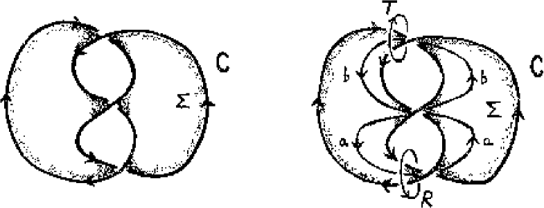
Figure 1. The trefoil knot with one of its Seifert surfaces.

In [16, p. 232], the authors assert that $H_{1}(S^{3}\setminus\Sigma;{\mathbb{R}})=0$ (equivalently $H_{1}(\Omega_{C}(\Sigma);{\mathbb{R}})=0$), but that $S^{3}\setminus\Sigma$ (equivalently, $\Omega_{C}(\Sigma)$) is not simply connected. The first claim is wrong. In fact, consider the two oriented loops $a$ and $b$ contained in $\Sigma$ and the two oriented loops $R$ and $T$ contained in $\Omega_{C}(\Sigma)$ drawn in Figure 1 (on the right). The surface $\Sigma$ is homeomorphic to a torus minus an open $2$–ball, and the homology classes of $a$ and of $b$ in $\Sigma$ form a basis of $H_{1}(\Sigma;{\mathbb{R}})$ (see also Figure 8.12 of [4, p. 243] to visualize these facts). Lefschetz Duality Theorem immediately implies that the homology classes of $R$ and of $T$ form a basis of $H_{1}(\Omega_{C}(\Sigma);{\mathbb{R}})$. In particular, this last space is non–trivial. Moreover, the trefoil knot is an example of fibred knot having the given Seifert surface as a fibre (this is carefully described in [61, p. 327])). Hence, $\Omega_{C}(\Sigma)$ is homeomorphic to $(\Sigma\setminus\partial\Sigma)\times(0,1)$ and has therefore the same homotopy type of $\Sigma$. Note that this fact confirms the above claim that $H_{1}(\Omega_{C}(\Sigma);{\mathbb{R}})$ and $H_{1}(\Sigma;{\mathbb{R}})$ are isomorphic.

The first argument above can be rephrased in a more physical fashion. Suppose $a$ is an ideally thin conductor, carrying a current of unitary intensity. Let ${\bf H}_{a}$ be the corresponding magnetic field. The restriction ${\bf H}^{\prime}_{a}$ of ${\bf H}_{a}$ to $S^{3}\setminus\Sigma$ is a curl–free smooth vector field, which does not have any scalar potential. In fact, the circulation of ${\bf H}^{\prime}_{a}$ along $R$ is $1$. In particular, by Stokes’ Theorem, the homology class of $R$ in $S^{3}\setminus\Sigma$ is not null. Similar considerations can be repeated for $b$ and $T$.

We believe that the following observation contains a possible source of this mistake. In Figure 2, it is drawn a compact connected orientable surface $B$ of ${\mathbb{R}}^{3}$ with boundary $R$ contained in $S^{3}\setminus C$ (see also Figure 8.13 of [4, p. 244]). The existence of such a surface implies that $R$ represents the null homology class in $H_{1}(S^{3}\setminus C;{\mathbb{R}})$. Then the restriction to $S^{3}\setminus\Sigma$ of any curl–free smooth vector field defined on the whole of $S^{3}\setminus C$ has null circulation along $R$. On the other hand, not every curl–free smooth vector fields on $S^{3}\setminus\Sigma$ can be extended to $S^{3}\setminus C$. Note also that the surface $B$ intersects in an essential way the Seifert surface $\Sigma$. These facts explain why the homology class of $R$ in $S^{3}\setminus C$ is null, while the homology class of $R$ in $S^{3}\setminus\Sigma$ is not. We will elaborate this remark in Section 5 below.

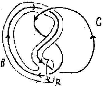
Figure 2. A null homologous cycle.

Example 3.4.

In their discussion about the relationship between homotopy and homology, Vourdas and Binns also consider the case of the Whitehead link (see Figure 3 above on the left). With notations as in Figure 3, they claim that the loop $R$ is homologically trivial and homotopically non–trivial in the complement of $C$ (see [5]). On the contrary, the sequence of moves described in Figure 3 shows that $R$ is homotopic (in the complement of $C$) to a loop $R^{\prime}$ which is clearly null–homotopic. In fact, as discussed in Subsection 2.6, since $R,R^{\prime}$ are loops in ${\mathbb{R}}^{3}\setminus C$ and $R$ can be continuosly deformed into $R^{\prime}$ without crossing $C$ (but crossing itself!), then $R$ and $R^{\prime}$ are homotopic in ${\mathbb{R}}^{3}\setminus C$. This implies, in particular, that $R$ bounds a singular $2$–disk in ${\mathbb{R}}^{3}\setminus C$. In fact, since $R$ and $C$ are not geometrically unlinked, $R$ cannot bound an embedded locally flat $2$–disk in ${\mathbb{R}}^{3}\setminus C$. As a consequence, it can be shown that $R$ and $R^{\prime}$ are not isotopic in ${\mathbb{R}}^{3}\setminus C$.

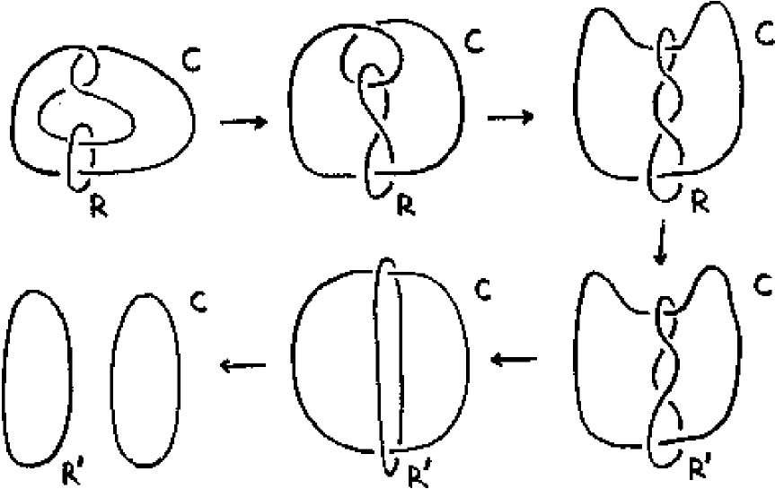
Figure 3. Homotoping $R$ to a trivial knot in ${\mathbb{R}}^{3}\setminus C$.

3.3. Elementary results about the algebraic topology of domains

Let $M$ be a compact smooth manifold. We say that $M$ is closed if its boundary is empty. By the classical Morse theory (see [54], [46]), if $M$ is closed, then it has the homotopy type of a finite CW complex of dimension $m={\rm dim}\ M$, which can be constructed by means of any Morse function on $M$. If $M$ is connected with non–empty boundary, then it has the homotopy type of a CW complex of dimension $<m$. This can be realized by means of any Morse function $f:(M,\partial M)\longrightarrow([0,1],\{1\})$ without local maxima. The same facts hold if $M$ is polyhedral. One can get a unified treatment by reformulating Morse theory in terms of handle decompositions theory, which makes sense also in the polyhedral setting (see [55], [62]). By Theorem 2.8, in our favourite case of spatial domains, we can adopt both points of view.

Since ${\mathbb{R}}$ is a field, an easy application of the Universal Coefficient Theorem for cohomology shows that, for every $k\in\mathbb{N}$, the singular $k$–cohomology module $H^{k}(M;{\mathbb{R}})$ of $M$ with coefficients in ${\mathbb{R}}$ is isomorphic to the dual space ${\rm Hom}(H_{k}(M;{\mathbb{R}}),{\mathbb{R}})$ of the corresponding singular homology module $H_{k}(M;{\mathbb{R}})$. Moreover, compactness of $M$ implies that, for every $k\in\mathbb{N}$, the $k$–th Betti number $b_{k}(M):=\dim H_{k}(M;{\mathbb{R}})$ of $M$ is finite, whence equal to $\dim H^{k}(M;{\mathbb{R}})$. In fact, by using the fundamental isomorphism between cellular (or simplicial) and singular homologies, it follows that $\dim H_{k}(M;{\mathbb{R}})$ is finite and vanishes for every $k>\dim M$. Similar results also hold for homology and cohomology with integer coefficients: $H_{n}(M;{\mathbb{Z}})$ and $H^{n}(M;{\mathbb{Z}})$ are finitely generated for every $n\in\mathbb{N}$ and trivial for $n>\dim M$. Hence, if we denote by $T_{n}(M)$ the submodule of finite–order elements of $H_{n}(M,{\mathbb{Z}})$, then $T_{n}(M)$ is finite and

$$H_{n}(M;{\mathbb{Z}})=\big{(}H_{n}(M;{\mathbb{Z}})/T_{n}(M)\big{)}\oplus T_{n}(M)\,.$$

Being finitely generated and torsion–free, the quotient $H_{n}(M;{\mathbb{Z}})/T_{n}(M)$ is isomorphic to ${\mathbb{Z}}^{r}$ for some $r\geq 0$; such a $r$ will be called the rank of $H_{n}(M;{\mathbb{Z}})$ and will be denoted by $r_{n}(M)$.

Since ${\mathbb{R}}$ is a field, the Universal Coefficient Theorem for homology ensures that $H_{n}(M;{\mathbb{R}})=H_{n}(M;{\mathbb{Z}})\otimes{\mathbb{R}}$, and this implies in turn that $r_{n}(M)=b_{n}(M)$. Let us now recall the definition of the Euler–Poincaré characteristic $\chi(M)$ of $M$:

$$\chi(M):=\sum_{n=0}^{\dim M}(-1)^{n}b_{n}(M)\,.$$

It is well–known that, if $c_{n}$ is the number of $n$–cells ($n$–simplexes) of any finite CW complex homotopy equivalent to (any triangulation of) $M$, then $\chi(M)$ admits the following combinatorial description:

$$\chi(M)=\sum_{n=0}^{\dim M}(-1)^{n}c_{n}\,.$$

We now list some elementary results that will prove useful later.

(1) Assume that $M$ is connected. Then $b_{0}(M)=1$. If $\dim M=m$ and $M$ has non–empty boundary, then $b_{m}(M)=0$. The last claim follows from the above–mentioned fact that $M$ has the homotopy type of a CW complex of stricly smaller dimension.

(2) If $M$ is a closed manifold of odd dimension $m=2n+1$, then $\chi(M)=0$. In fact, by using the “dual” CW complexes associated to $f$ and $-f$, where $f$ is a suitable Morse function on $M$, one realizes that the respective numbers of cells verify the relations $c_{i}=c^{*}_{m-i}$, and hence the result easily follows from the combinatorial formula for the characteristic. If $M$ is triangulated, one can use the dual cell decomposition of a given triangulation. This is a primitive manifestation of the Poincaré duality on $M$.

(3) If $M$ is a connected manifold with non–empty boundary $\partial M$, then we can construct the double $D(M)$ of $M$, by glueing two copies of $M$ along their boundaries via the identity map. Then $D(M)$ is closed and

$$\chi(D(M))=2\chi(M)-\chi(\partial M)\,.$$

In the case of triangulable manifolds (like spatial domains), the latter equality follows easily by considering a triangulation of $(M,\partial M)$, that induces a triangulation of the double, and by using the combinatorial formula for $\chi$. Hence, if $\dim M$ is odd, then $\chi(\partial M)=2\chi(M)$ is even. Moreover, we observe that

$$\chi(\partial M)=\sum_{i}\chi(S_{i})\,,$$

where the $S_{i}$’s are the boundary components of $M$.

Let us now specialize to domains.

(4) As already mentioned, if $\Omega\subset{\mathbb{R}}^{3}$ is a domain with smooth boundary, then $\Omega$ is homotopically equivalent to $\overline{\Omega}$, so $b_{n}(\Omega)=b_{n}(\overline{\Omega})$ for every $n\in\mathbb{N}$. Since $\overline{\Omega}$ is a compact smooth $3$-manifold with non–empty boundary, we deduce from point (1) above that

$$\chi(\Omega)=\chi(\overline{\Omega})=1-b_{1}(\Omega)+b_{2}(\Omega)\,.$$

(5) If $M=S$ is a smooth surface in ${\mathbb{R}}^{3}$, then $b_{0}(S)=1=b_{2}(S)$, and $S$ bounds $\overline{\Omega(S)}$. In particular, by point (3) above, $b_{1}(S)=2-\chi(S)$ is even. The non–negative integer

$$g(S):=\frac{b_{1}(S)}{2}$$

is called genus of $S$. A basic classification theorem of orientable surfaces (see [46]) says that two compact orientable surfaces are diffeomorphic if and only if they have the same genus. In particular, $S$ is a smooth 2–sphere if and only if $g(S)=0$.

(6) If $\Omega\subset{\mathbb{R}}^{3}$ is a domain whose boundary consists of the disjoint union of smooth surfaces $S_{0},\ldots,S_{h}$, then, by points (3) and (5) above, it holds:

$$\chi(\Omega)=\frac{\chi(\partial M)}{2}=\frac{1}{2}\sum_{i=0}^{h}\chi(S_{i})=\frac{1}{2}\sum_{i=0}^{h}\big{(}2-2g(S_{i})\big{)}=h+1-\sum_{i=0}^{h}g(S_{i})\,.$$

3.4. Proof of Theorem 3.1

Let $\Omega$ be a domain with locally flat boundary such that $H^{1}(\Omega;{\mathbb{R}})=0$. We know that it is not restrictive to assume that $\Omega$ has smooth boundary. We denote by $S_{0},\ldots,S_{h}$ the boundary components of $\partial\Omega$, keeping notations from Lemma 2.4.

Let us set $b_{1}:=b_{1}(\Omega)$, $b_{2}:=b_{2}(\Omega)$. As a consequence of the Universal Coefficient Theorem, our hypothesis is exactly equivalent to say that $b_{1}=0$. By point (4) above, this is equivalent to $\chi(\Omega)=1+b_{2}$ as well. Together with the equality $\chi(\Omega)=h+1-\sum_{i=0}^{h}g(S_{i})$ proved above, this implies that

(1) $$h-\sum_{i=0}^{h}g(S_{i})=b_{2}\geq 0\ .$$

The proof proceeds now by induction on $h\geq 0$. If $h=0$, then we have $-g(S_{0})\geq 0$, so $g(S_{0})=0$ and $S_{0}$ is a smooth 2–sphere embedded in $S^{3}$. Hence, in this case, our theorem reduces to the celebrated Alexander Theorem (1924) [20] (see also [44] for a very accessible proof in the case of smooth spheres, rather than polyhedral ones as in the original paper by Alexander). If $h\geq 1$, then equation (1) implies that $g(S_{j_{0}})=0$ for at least one $j_{0}\in\{0,\ldots,h\}$. Suppose $j_{0}\geq 1$. Let us denote by $\Omega^{0}$ the domain $\Omega^{0}=\Omega\cup\overline{\Omega(S_{j_{0}})}$ obtained by capping–off the boundary sphere $S_{j_{0}}$ of $\Omega$ with the 3–disk $\overline{\Omega(S_{j_{0}})}$. An elementary application of the Mayer–Vietoris Theorem (see e.g. [43]) shows that $\Omega^{0}$ is a domain with $(h-1)$ boundary components such that $H^{1}(\Omega^{0};{\mathbb{R}})=0$, and this allows us to conclude by induction. If $j_{0}=0$, then the same proof applies, after defining $\Omega^{0}$ as the domain obtained by filling $\Omega$ (in $S^{3}$) with the 3–disk $\overline{\Omega^{*}(S_{0})}$.  $\Box$

Remark 3.5.

Theorem 3.1 does not hold in general if we don’t assume $\Omega$ to have locally flat boundary. In fact, on one hand, the Jordan–Brower Separation Theorem (which is more sophisticated than Proposition 2.2, see [25]) establishes that every topological 2–sphere $S$ embedded in $S^{3}$ disconnects $S^{3}$ in two domains each of which has trivial singular $1$–homology module. On the other hand, Alexander again ([19, 21], see also [61, p. 76 and p. 81]) produced celebrated examples of non–locally flat topological 2–spheres whose complement in $S^{3}$ consists of domains one of which (or even both of which) is not simply connected.

Remark 3.6.

A smooth compact connected $3$–manifold $M$ with non–empty boundary is a ${\mathbb{Z}}$–homology disk (resp. ${\mathbb{R}}$–homology disk) if its homology modules with coefficients in ${\mathbb{Z}}$ (resp. in ${\mathbb{R}}$) are trivial, except that in dimension 0 (so a ${\mathbb{Z}}$–homology disk is necessarily a ${\mathbb{R}}$–homology disk). Non–simply connected ${\mathbb{R}}$–homology disks are easily constructed by removing a small genuine $3$–ball from closed $3$–manifolds with finite (but non–trivial) fundamental group such as the projective space $\mathbb{P}^{3}({\mathbb{R}})$ or any lens space $L(p,q)$ (see [61, p. 233]). In the same spirit, a non–simply connected ${\mathbb{Z}}$–homology disk can be obtained by removing a genuine $3$–ball from a closed non–simply connected $3$–manifold having trivial 1–dimensional ${\mathbb{Z}}$–homology. The first example of such a manifold is due to Poincaré. Theorem 3.1 implies that non–simply connected ${\mathbb{R}}$–homology disks cannot be embedded in $S^{3}$.

Remark 3.7.

Even in the locally flat case, the conclusions of Theorem 3.1 are no longer true when dealing with domains in higher dimensional Euclidean space. For example, the projective plane $\mathbb{P}^{2}({\mathbb{R}})$ can be emdedded in ${\mathbb{R}}^{4}$, and a tubular neighbourhood of the image of such an embedding is a 4–dimensional ${\mathbb{R}}$–homology disk with fundamental group isomorphic to ${\mathbb{Z}}/2{\mathbb{Z}}$.

We end this section with an open question (as far as we know):

Question 3.8.

Let $\Omega$ be a not necessarily bounded domain with smooth boundary. Assume that $H^{1}(\Omega;{\mathbb{R}})=0$. Does it hold anyway that $\Omega$ is simply connected?

4. Helmholtz domains

Let us give a definition that covers many current instances in the literature about Helmholtz cuts method (see also Remark 4.6).

Definition 4.1.

A domain $\Omega\subset{\mathbb{R}}^{3}$ with locally flat boundary is Helmholtz if there exists a finite family ${\mathcal{F}}=\{\Sigma_{i}\}$ (called cut–system for $\Omega$) of disjoint properly embedded (connected) surfaces in $(\overline{\Omega},\partial\Omega)$, such that every connected component $\Omega^{0}$ of $\Omega_{C}({\mathcal{F}})$ (i.e. the disjoint union of domains obtained by cut/open simultaneouosly along all the $\Sigma_{i}$’s) satisfies $H^{1}(\Omega^{0};{\mathbb{R}})=0$.

We are going to provide an exhaustive and simple characterization of Helmholtz domains (and of their cut–systems). We say that a cut–system for $\Omega$ is minimal if it does not properly contain any cut–system for $\Omega$. Of course, every cut–system contains a minimal cut–system.

Lemma 4.2.

Suppose ${\mathcal{F}}$ is a minimal cut–system for $\Omega$. Then $\Omega_{C}({\mathcal{F}})$ is connected. In particular, every surface of ${\mathcal{F}}$ has non–empty boundary.

Proof.

Let $\Omega_{1},\ldots,\Omega_{k}$ be the connected components of $\Omega_{C}({\mathcal{F}})$ and suppose by contradiction $k\geq 2$. Then we can find a connected surface $\Sigma_{0}\in{\mathcal{F}}$ which lies “between” two distinct $\Omega_{i}$’s. We will now show that the family ${\mathcal{F}}^{\prime}={\mathcal{F}}\setminus\{\Sigma_{0}\}$ is a cut–system for $\Omega$, thus obtaining the desired contradiction.

Up to reordering the $\Omega_{i}$’s, we may suppose that (parallel copies of) $\Sigma_{0}$ lie in the boundary of both $\Omega_{k-1}$ and $\Omega_{k}$, so that $\Omega_{C}({\mathcal{F}}^{\prime})=\Omega^{\prime}_{1}\cup\ldots\cup\Omega^{\prime}_{k-1}$, where $\Omega^{\prime}_{i}=\Omega_{i}$ for every $i\in\{1,\ldots,k-2\}$, $\Sigma_{0}$ is properly embedded in $\Omega^{\prime}_{k-1}$ and $\Omega_{k-1}\cup\Omega_{k}$ is obtained by cutting $\Omega^{\prime}_{k-1}$ along $\Sigma_{0}$. Since ${\mathcal{F}}$ is a cut–system for $\Omega$, the modules $H^{1}(\Omega_{k-1};{\mathbb{R}})$ and $H^{1}(\Omega_{k};{\mathbb{R}})$ are null. By Theorem 3.1, it follows that $\Omega_{k-1}$ and $\Omega_{k}$ are simply connected. But $\Sigma_{0}$ is connected, so an easy application of Van–Kampen’s Theorem (see e.g. [43]) ensures that $\Omega^{\prime}_{k-1}$ is also simply connected, whence $H^{1}(\Omega^{\prime}_{k-1};{\mathbb{R}})=0$. Therefore ${\mathcal{F}}^{\prime}$ is a cut–system for $\Omega$.

We have thus proved the first statement of the lemma. Now the conclusion follows from the fact that every smooth surface $S\subset\overline{\Omega}$ without boundary disconnects $S^{3}$ (see Proposition 2.2), whence a fortiori $\Omega$. ∎

Definition 4.3.

A 3–dimensional $1$–handle is a $3$–manifold $M$ homeomorphic to $D^{2}\times[0,1]$ on which there is fixed a distinguished subspace $A\subset M$ such that the pair $(M,A)$ is homeomorphic to the pair $(D^{2}\times[0,1],D^{2}\times\{0,1\})$. The connected components of $A$ are the attaching $2$–disks of $M$, while if $B\subset M$ corresponds to $D^{2}\times\{1/2\}$ under a homeomorphism $(M,A)\cong(D^{2}\times[0,1],D^{2}\times\{0,1\})$, then $B$ is a co–core of $M$. A handlebody $\overline{H}$ in $S^{3}$ is the closure of a domain $H\subset S^{3}$ with connected locally flat boundary (called an open handlebody), which decomposes as the disjoint union of $3$–disks (the $0$–handles of $\overline{H}$) together with a disjoint union of 1–handles embedded in $S^{3}$ in such a way that the following conditions hold: the internal part of every $1$–handle is disjoint from the internal part of every $0$–handle, every attaching $2$–disk of every $1$–handle lies on the spherical boundary of some $0$–handle, and there are no further intersections between $0$– and $1$– handles (in the smooth case some “rounding the corners” procedure is understood).

Remark 4.4.

It is readily seen that a subset $\overline{H}$ of $S^{3}$ is a handlebody if and only if it is equal to a regular neighbourhood of a finite connected spatial graph $\Gamma$ (i.e. a 1–dimensional compact connected polyhedron) in $S^{3}$. $\Gamma$ is called a spine of $\overline{H}$.

Every open handlebody $H$ is Helmholtz: a cut–system ${\mathcal{M}}$ for $H$ is easily contructed by taking one co–core for every $1$–handle of $\overline{H}$, since in this case the result $H_{C}({\mathcal{M}})$ of cutting $H$ along ${\mathcal{M}}$ is just the family of the internal parts of the $0$–handles of $\overline{H}$, that are 3–balls. It is not hard to see that, for suitable subfamilies of these co–cores, the result of cut/open consists of just one 3–ball. We will refer to such a subfamily of co–cores as a minimal system of meridian $2$–disks for $H$. An easy argument using the Euler–Poincaré characteristic shows that the number $g(\overline{H})$ of $2$–disks in a minimal system of meridian $2$–disks for $H$ equals the genus $g(\partial H)$ of $\partial H$, and is, in particular, independent from the handle–decomposition of $\overline{H}$. We will call $g(\overline{H})$ the genus of $\overline{H}$. Via “handle sliding”, it can be easily shown that two handlebodies are (abstractly) homeomorphic if and only if they have the same genus. Recall that 3–disks are the handlebodies of genus $0$.

We are now ready to state the main result of this section. We denote by $\Omega$ a domain of ${\mathbb{R}}^{3}$ with locally flat boundary and by $S_{0},\ldots,S_{h}$ the connected components of $\partial\Omega$, ordered as in Lemma 2.4.

Theorem 4.5.

$\Omega$ is a Helmholtz domain if and only if the following two conditions hold:

• The domains $\Omega(S_{0})$ and $\Omega^{*}(S_{j})$, $j=1,\dots,h$, are open handlebodies in $S^{3}$.

• Every $\Omega(S_{j})$, $j=1,\dots,h$, is contained in a $3$–disk of $S^{3}$, embedded in $\Omega(S_{0})$, and these $3$–disks are pairwise disjoint.

Moreover, if $\Omega$ is Helmholtz, then there exists a cut–system ${\mathcal{F}}$ for $\Omega$ such that each element of ${\mathcal{F}}$ is a properly embedded $2$–disk in $(\overline{\Omega},\partial\Omega)$, and $\Omega_{C}({\mathcal{F}})$ consists of one “external” $3$–ball with some “internal” pairwise disjoint $3$–disks removed. In particular, $\Omega_{C}({\mathcal{F}})$ is connected $($whence simply connected$)$.

Proof. We can suppose as usual that $\Omega$ has smooth boundary. Assume that $\Omega$ verifies $(1)$ and $(2)$. Thanks to these conditions, it is possible to choose a minimal system ${\mathcal{M}}_{0}$ of meridian $2$–disks for $\Omega(S_{0})$ and, for every $i\in\{1,\ldots,h\}$, a minimal system ${\mathcal{M}}_{i}$ of meridian $2$–disks for $\Omega^{\ast}(S_{i})$ in such a way that $2$–disks belonging to distinct ${\mathcal{M}}_{i}$’s, $i=0,1,\ldots,h$, are pairwise disjoint. It is now readily seen that $\bigcup_{i=0}^{h}{\mathcal{M}}_{i}$ provides the cut–system required in the last statement of the theorem. In particular, $\Omega$ is Helmholtz.

Let us concentrate on the converse implication. Denote by ${\mathcal{F}}$ an arbitrary cut–system for the Helmholtz domain $\Omega$. Accordingly to the definition of the cut/open operation along ${\mathcal{F}}$, we have $\Omega_{C}({\mathcal{F}})=\Omega\setminus\bigcup_{\Sigma\in{\mathcal{F}}}U_{\Sigma}$, where each $U_{\Sigma}$ is a bicollar of $(\Sigma,\partial\Sigma)$ in $(\overline{\Omega},\partial\Omega)$, and these bicollars are pairwise disjoint. Hence $\overline{\Omega}$ can be reconstructed starting from $\overline{\Omega_{C}({\mathcal{F}})}$ by attaching to its boundary the $U_{\Sigma}$’s along the surfaces $\Sigma^{+}$ and $\Sigma^{-}$ corresponding to $\Sigma\times\{\pm 1\}$ in $\Sigma\times[-1,1]\cong U_{\Sigma}$. By Theorem 3.1, every component of $\Omega_{C}({\mathcal{F}})$ consists of an “external” 3–ball with some “internal” pairwise disjoint 3–disks removed, so the boundary components of $\Omega_{C}({\mathcal{F}})$ are spheres. It follows that every surface $\Sigma$ is planar, whence homeomorphic either to the $2$–sphere or to $D^{2}_{k}$ for some non–negative integer $k$, where $D^{2}_{k}$ is the closure in ${\mathbb{R}}^{2}$ of a $2$–disk $D^{2}$ with $k$ disjoint $2$–disks removed from its interior.

We will conclude the proof of the theorem in two steps. We will first assume that all the surfaces of a given cut–system ${\mathcal{F}}$ of the Helmholtz domain $\Omega$ are $2$–disks. Next we will show how every arbitrarily given cut–system ${\mathcal{F}}$ can be eventually replaced with one consisting of $2$–disks only.

Step 1. Suppose that ${\mathcal{F}}$ is a cut–system for $\Omega$ consisting of $2$–disks only. By Lemma 4.2, up to replacing ${\mathcal{F}}$ with a minimal cut–system contained in ${\mathcal{F}}$, we may suppose that $\Omega_{C}({\mathcal{F}})$ is connected, so that it consists of just one “external” $3$–ball $B_{0}$ with some “internal” pairwise disjoint $3$–disks removed. Observe that we can reconstruct $\overline{\Omega}$ starting from $\overline{\Omega_{C}({\mathcal{F}})}$ simply by attaching to $\overline{\Omega_{C}({\mathcal{F}})}$ one $1$–handle for each $2$–disk in ${\mathcal{F}}$: the attached $1$–handle just coincides with the removed tubular neighbourhood $D^{2}\times[0,1]$ of such a $2$–disk in $\overline{\Omega}$, in such a way that the attaching $2$–disks are identified with $D^{2}\times\{0,1\}$. Let us consider first the $1$–handles attached to $\overline{B}_{0}$. By the very definitions, the internal part $\Omega(S_{0})$ of the union of $\overline{B}_{0}$ with such $1$–handles is an open handlebody. Let $T_{1},\ldots,T_{h}$ be the internal boundary spheres of $\Omega_{C}({\mathcal{F}})$ and, for each $j\in\{1,\ldots,h\}$, let $B_{j}$ be the internal part of the $3$–disk $D_{j}$ bounded by $T_{j}$. Now $\overline{\Omega}$ is obtained by attaching to each $T_{j}$ some 1–handles contained in the corresponding $D_{j}$. This description provides a realization of each $\Omega^{*}(S_{j})$, $j=1,\dots,h$, as an open handlebody. Note that every $\Omega(S_{j})$, $j=1,\dots,h$, is contained in the corresponding $B_{j}$. Moreover, ${\mathcal{F}}$ coincides with the family obtained by taking one co–core $2$–disk for each added $1$–handle. This completes the proof in the special case.

Step 2. Denote by ${\mathcal{F}}$ an arbitrary cut–system for the Helmholtz domain $\Omega$. Let us show that it is possible to replace ${\mathcal{F}}$ with a cut–system containing only $2$–disks.

Up to replacing ${\mathcal{F}}$ with a minimal cut–system, we may assume that every element of ${\mathcal{F}}$ is homeomorphic to $D^{2}_{k}$ for some non–negative $k$, and that $\Omega_{C}({\mathcal{F}})$ is connected, so that it consists of just one external $3$–ball $B_{0}$ with some internal pairwise disjoint $3$–disks $D_{1},\ldots,D_{l}$ removed. We denote by $T_{0}$ the $2$–sphere bounding $B_{0}$ and by $T_{i}$ the $2$–sphere bounding $D_{i}$, $i=1,\ldots,l$, and we observe that, under the above assumptions, for every surface $\Sigma\in{\mathcal{F}}$, there exists $i\in\{0,\ldots,l\}$ such that both $\Sigma^{+}$ and $\Sigma^{-}$ are contained in $T_{i}$.

We will now show that, if $\Sigma\in{\mathcal{F}}$ is homeomorphic to $D^{2}_{k}$ for some $k\geq 1$, then we can obtain a new cut–system ${\mathcal{F}}^{\prime}$ from ${\mathcal{F}}$ by replacing $\Sigma$ with two properly embedded $2$–disks. Such a cut–system will contain a minimal cut–system ${\mathcal{F}}^{\prime\prime}$ with a smaller number (with respect to ${\mathcal{F}}$) of non–diskal surfaces. Together with an obvious inductive argument, this will easily imply that, if $\Omega$ is Helmholtz, then it admits a cut–system consisting of $2$–disks only, whence the conlusion. So let $T_{i}$ be the component of $\partial\Omega_{C}({\mathcal{F}})$ containing $\Sigma^{+}$ and $\Sigma^{-}$, choose a boundary component $\gamma$ of $D^{2}_{k}$ and denote by $\gamma^{+}$, $\gamma^{-}$ the curves on $T_{i}$ corresponding to $\gamma\times\{-1\}$, $\gamma\times\{1\}$ under the identification of $\Sigma\times\{\pm 1\}$ with $\Sigma^{+}\subset T_{i}$ and $\Sigma^{-}\subset T_{i}$. Now if $D_{{\gamma}^{+}}$ is the $2$–disk on $T_{i}$ bounded by $\gamma^{+}$ and containing $\Sigma^{+}$,we slightly push the internal part of $D_{\gamma^{+}}$ into $\Omega_{C}({\mathcal{F}})$ thus obtaining a $2$–disk $D^{+}$ properly embedded in $\Omega_{C}({\mathcal{F}})$ such that $\partial D^{+}=\gamma^{+}$ (see Figure 4). The same procedure applies to $\gamma^{-}$ providing a $2$–disk $D^{-}$ properly embedded in $\Omega_{C}({\mathcal{F}})$, and of course we may also assume that $D^{+}$ and $D^{-}$ are disjoint. Also observe that by construction both $D^{+}$ and $D^{-}$ are disjoint from every surface in ${\mathcal{F}}$.

We now set ${\mathcal{F}}^{\prime}=({\mathcal{F}}\setminus\{\Sigma\})\cup\{D^{+},D^{-}\}$. It is easy to see that $\Omega_{C}({\mathcal{F}}^{\prime})$ is given by the disjoint union of a domain homeomorphic to $\Omega_{C}({\mathcal{F}})$ and a domain $\Omega^{\prime}$ homeomorphic to the internal part of

$$\left(D^{2}\times[-1,-1+\varepsilon]\right)\cup\left(D^{2}_{k}\times[\varepsilon,1-\varepsilon]\right)\cup\left(D^{2}\times[1-\varepsilon,1]\right)\ .$$

Now $\Omega^{\prime}$ is homeomorphic to a $3$–ball with $k$ pairwise disjoint $3$–disks removed, and is therefore simple (in the sense of Theorem 3.1). Together with the fact that $\Omega_{C}({\mathcal{F}})$ is simple, this implies that ${\mathcal{F}}^{\prime}$ is a cut–system for $\Omega$. $\Box$

Figure 4. Diskal vs planar co–cores: the dashed lines represent $\Sigma$, $\Sigma^{+}$ and $\Sigma^{-}$, while the thickened strings represent the “holes” of $D_{k}^{2}\times[-1,1]$ (here $k=2$).

Remark 4.6.

Bearing in mind the proof of Theorem 4.5, we can now list some equivalent reformulations of the Helmholtz condition for spatial domains.

$(1)$ A domain $\Omega$ of ${\mathbb{R}}^{3}$ with locally flat boundary is Helmholtz if and only if there exists a finite family ${\mathcal{S}}=\{S_{i}\}$ of simple domains of ${\mathbb{R}}^{3}$ $($in the sense of Theorem 3.1$)$, whose closures are pairwise disjoint, such that $\overline{\Omega}$ can be constructed starting from the union of the closures of the $S_{i}$’s, by attaching some pairwise disjoint $1$–handles to the boundary spheres of such a union. In addition $($and equivalently$)$, one may suppose that ${\mathcal{S}}$ consists of a single simple domain.

$(2)$ A domain $\Omega$ of ${\mathbb{R}}^{3}$ with locally flat boundary is Helmholtz if there exists a finite family $D_{i}$, $i=1,\ldots,\ell$, of properly embedded $2$–disks in $(\overline{\Omega},\partial\Omega)$ such that $\Omega\setminus\bigcup_{i=1}^{\ell}D_{i}$ is simply connected. In particular, as already mentioned in Lemma 4.2, we would get an equivalent definition of Helmholtz domains if we admitted only cutting surfaces with non–empty boundary.

$(3)$ Suppose that $\Omega$ is Helmholtz. Then $\Omega$ is weakly–Helmholtz, and every cut–system for $\Omega$ is a weak cut–system for $\Omega$ (see Section 5 for the definitions of weakly–Helmholtz domain and weak cut–system). In particular, Proposition 5.18 implies that every cut–system for $\Omega$ contains at least $b_{1}(\Omega)$ surfaces. On the other hand, if ${\mathcal{F}}=\{D_{1},\ldots,D_{\ell}\}$ is a cut–system for $\Omega$ consisting of properly embedded $2$–disks in $(\overline{\Omega},\partial\Omega)$ such that $\Omega\setminus\bigcup_{i=1}^{\ell}D_{i}$ is simply connected, then an easy application of the Mayer–Vietoris Theorem implies that $\ell$ is equal to $b_{1}(\Omega)$. Therefore $b_{1}(\Omega)$ provides the optimal lower bound on the number of surfaces contained in the cut–systems for $\Omega$.

In Figure 5, it is drawn a “typical example” of Helmholtz domain: each big circle containing smaller circles represents an “external” $3$–ball with some “internal” pairwise disjoint $3$–disks removed, and the remaining bands represent the attached $1$–handles.

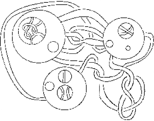
Figure 5. A Helmholtz domain.

In some sense, Theorem 4.5 should be considered a negative result, as it shows that the topology of Helmholtz domains is forced to be very simple. The following corollary provides an evidence for this claim. Its proof follows immediately from Theorem 4.5 and the discussion in Subsection 2.3. For simplicity, we say that a link $L$ of $S^{3}$ is Helmholtz if its complement–domain $\mathsf{C}(L)$ is.

Corollary 4.7.

Given a link $L$ in $S^{3}$, the following assertions are equivalent:

• $L$ is Helmholtz.

• $L$ is trivial.

• $\mathsf{B}(L)$ is Helmholtz.

The trefoil knot $L$ is not trivial, so the associated box–domain $\mathsf{B}(L)$, drawn in Figure 6, is a simple example of a domain of ${\mathbb{R}}^{3}$ with smooth boundary, which is not Helmholtz.

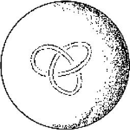
Figure 6. A box–domain of a trefoil knot is not Helmholtz.

4.1. Unknotting reimbedding

The handlebodies occurring in Theorem 4.5 are in general knotted. Let us make precise this notion. A handlebody $\overline{H}$ is unknotted if, up to ambient isotopy, it admits a planar spine (in the sense of Remark 4.4) contained in ${\mathbb{R}}^{2}\subset{\mathbb{R}}^{3}\subset S^{3}$. Thanks to a celebrated theorem of Waldhausen [71, 64], this is equivalent to the fact that also the complementary domain in $S^{3}$ is a handlebody: in fact, a decomposition of $S^{3}$ into complementary handlebodies is a so–called Heegaard splitting of $S^{3}$, and the Heegaard splitting of the sphere has been proved to be unique up to isotopy. By extending the notions of Subsection 2.3, we define a link of handlebodies in $S^{3}$ to be the union of a finite family of disjoint handlebodies. Such a link is trivial if all handlebodies of the family are unknotted and geometrically unlinked, that is contained in pairwise disjoint 3–disks of $S^{3}$.

Every (possibly knotted) handlebody can be reimbedded in $S^{3}$ onto an unknotted one. We can apply separately this fact to the handlebodies $\Omega(S_{0})$ and $\Omega^{*}(S_{j})$, $j=1,\ldots,h$, of Theorem 4.5 and get the following:

Corollary 4.8.

A domain $\Omega$ of ${\mathbb{R}}^{3}$ with locally flat boundary is Helmholtz if and only if it can be reimbedded in $S^{3}$ onto a domain $\Omega^{\prime}$, which is the complement of a trivial link of handlebodies.

As an exercise one can see how to realize such an unknotted reimbedding of the domain of Figure 5, just by changing some (over/under) crossings of the bands representing the $1$–handles.

By comparing the previous corollary with the following general (and non–trivial) reimbedding theorem due to Fox [34], we have a further evidence of the topological simplicity of Helmholtz domains.

Theorem 4.9 (Fox reimbedding Theorem).

Every domain $\Omega$ of $S^{3}$ with locally flat boundary can be reimbedded in $S^{3}$ onto a domain $\Omega^{\prime}$, which is the complement of a link of handlebodies.

5. Weakly–Helmholtz domain

In this section, we propose and discuss a strictly weaker notion of “domains that simplify after suitable cuts”. We believe that the notion we are introducing captures the substance of the philosophy of Helmholtz cuts, with the advantage of covering a much wider range of topological models.

In order to save words, from now on, if $M$ is a compact oriented 3–manifold with locally flat boundary, we call system of surfaces in $M$ any finite family ${\mathcal{F}}=\{\Sigma_{i}\}$ of disjoint oriented connected surfaces properly embedded in $M$. We stress that every element of a system of surfaces is connected and oriented, and that the elements of such a system are pairwise disjoint. We begin with a definition in the spirit of condition (b) of Section 3 (see also Remark 5.20).

Definition 5.1.

A domain $\Omega$ with locally flat boundary is weakly–Helmholtz if it admits a system of surfaces ${\mathcal{F}}$ (called a weak cut–system for $\Omega$) such that, for every connected component $\Omega^{0}$ of $\Omega_{C}({\mathcal{F}})$, the following condition holds: the restriction to $\Omega^{0}$ of every curl–free smooth vector field defined on the whole of $\Omega$ is the gradient of a smooth function on $\Omega^{0}$.

It readily follows from the preceding definition and from Theorem 4.5 that every Helmholtz domain is weakly–Helmholtz.

Just as we did in Section 3, let us give some topological reformulations of the above definition. As usual, it is not restrictive to work in the framework of domains with smooth boundary. So let $\Omega$ be a domain with smooth boundary, let ${\mathcal{F}}$ be a system of surfaces in $\overline{\Omega}$ and let $\Omega_{1},\ldots,\Omega_{k}$ be the connected components of $\Omega_{C}({\mathcal{F}})$. For $j\in\{1,\ldots,k\}$, let also $i_{j}:\Omega_{j}\longrightarrow\Omega$ be the inclusion. Then ${\mathcal{F}}$ is a weak cut–system for $\Omega$ if and only if one of the following equivalent conditions hold:

($\beta_{1}$) For every $j\in\{1,\ldots,k\}$, the image of $i_{j}^{*}:H^{1}_{DR}(\Omega)\longrightarrow H^{1}_{DR}(\Omega_{j})$ vanishes.

($\beta_{2}$) For every $j\in\{1,\ldots,k\}$, the image of $i_{j}^{*}:H^{1}(\Omega;{\mathbb{R}})\longrightarrow H^{1}(\Omega_{j};{\mathbb{R}})$ vanishes.

($\beta_{3}$) For every $j\in\{1,\ldots,k\}$, the image of $(i_{j})_{*}:H_{1}(\Omega_{j};{\mathbb{R}})\longrightarrow H_{1}(\Omega;{\mathbb{R}})$ vanishes.

The fact that ${\mathcal{F}}$ is a weak cut–system for $\Omega$ if and only if $(\beta_{1})$ holds is a consequence of the canonical isomorphism between vector fields and 1–forms, the equivalence between $(\beta_{1})$ and $(\beta_{2})$ follows from the naturality of de Rham’s isomorphism, and the equivalence between $(\beta_{2})$ and $(\beta_{3})$ depends on the duality between cohomology and homology.

5.1. More results about the algebraic topology of domains

Before studying weakly–Helmholtz domains, it is convenient to develop a bit more of information about the algebraic topology of an arbitrary domain. While Theorem 4.5 provides an exhaustive description of Helmholtz domains, the classification of weakly–Helmholtz domains appears to be a quite difficult issue. In order to obtain some partial results in this direction, we will use less elementary (but still “classical”) tools such as relative homology and Lefschetz Duality Theorem. In what follows, we will assume that the reader has some familiarity with such notions and results, which are exhaustively described for instance in [43]. However, in order to preserve as much as possible the geometric (rather than algebraic) flavour of our arguments, we will often describe algebraic notions in terms of geometric ones via an extensive use of transversality. More precisely, we will often exploit the fact that, if $M$ is a smooth oriented $n$–dimensional manifold with (possibly empty) boundary $\partial M$, where $n=2,3$, then every $k$–dimensional (relative) homology class in $(M,\partial M)$ with integer coefficients can be geometrically represented by a smooth oriented closed $k$–manifold (properly) embedded in $M$. Moreover, the algebraic intersection between a $k$–dimensional and a $(n-k)$–dimensional class (which plays a fundamental rôle in several duality theorems) can be realized geometrically by taking transverse geometric representatives of the classes involved and counting the intersection points with suitable signs depending on orientations.

We now fix a domain $\Omega\subset{\mathbb{R}}^{3}$ with smooth boundary. Define $B:=S^{3}\setminus\overline{\Omega}$ and observe that $\partial\Omega=\overline{\Omega}\cap\overline{B}$ is the common smooth boundary of $\Omega$ and $B$. Since $\partial\Omega$ admits a bicollar, we may apply the Mayer–Vietoris machinery to the splitting $S^{3}=\overline{\Omega}\cup\overline{B}$, obtaining the short exact sequences

(2) $$H_{2}(\partial\Omega;{\mathbb{Z}})\longrightarrow H_{2}(\overline{\Omega};{\mathbb{Z}})\oplus H_{2}(\overline{B};{\mathbb{Z}})\longrightarrow H_{2}(S^{3};{\mathbb{Z}})=0$$

and

(3) $$0=H_{2}(S^{3};{\mathbb{Z}})\longrightarrow H_{1}(\partial\Omega;{\mathbb{Z}})\longrightarrow H_{1}(\overline{\Omega};{\mathbb{Z}})\oplus H_{1}(\overline{B};{\mathbb{Z}})\longrightarrow H_{1}(S^{3};{\mathbb{Z}})=0\ .$$

As an immediate consequence, we get the following lemma.

Lemma 5.2.

The maps $i_{\ast}\colon H_{1}(\partial\Omega;{\mathbb{Z}})\longrightarrow H_{1}(\overline{\Omega};{\mathbb{Z}})$ and $i_{\ast}\colon H_{2}(\partial\Omega;{\mathbb{Z}})\longrightarrow H_{2}(\overline{\Omega};{\mathbb{Z}})$, induced by the inclusion $i\colon\partial\Omega\hookrightarrow\overline{\Omega}$, are surjective.

Remark 5.3.

We sketch here a further geometric and more intuitive proof of the last lemma. Every class in $H_{1}(\overline{\Omega};{\mathbb{Z}})$ can be represented by a knot $C$ embedded in $\Omega$. Let $S\subset S^{3}$ be a Seifert surface for $C$, which we can assume to be transverse to $\partial\Omega$. Then $S\cap\overline{\Omega}$ realizes a cobordism between $C$ and a smooth curve contained in $\partial\Omega$, thus proving that $C$ is homologous to a $1$–cycle in $\partial\Omega$.

Every class in $H_{2}(\overline{\Omega};{\mathbb{Z}})$ can be represented by the disjoint union of a finite number of compact smooth orientable surfaces embedded in $\Omega$. Every such surface necessarily separates $S^{3}$ (see Proposition 2.2), whence $\Omega$, and is therefore homologically equivalent to a linear combination of boundary components.

Recall that, if we denote by $T_{n}(\overline{\Omega})$ the submodule of finite–order elements of $H_{n}(\overline{\Omega},{\mathbb{Z}})\cong H_{n}(\Omega;{\mathbb{Z}})$, then $T_{n}(\overline{\Omega})$ is finite for every $n\in\mathbb{N}$ and trivial for every $n>2$.

Lemma 5.4 (see also [12]).

It holds: $T_{n}(\overline{\Omega})=0$ for every $n\in\mathbb{N}$.

Proof. Of course, it is sufficient to consider the cases $n=0,1,2$. Since the $0$–dimensional homology module of any topological space is free, we have $T_{0}(\overline{\Omega})=0$. Moreover, the short exact sequence (3) implies that $H_{1}(\overline{\Omega};{\mathbb{Z}})$ is isomorphic to a submodule of the free ${\mathbb{Z}}$–module $H_{1}(\partial\Omega;{\mathbb{Z}})$, and is therefore free. Finally, by the Lefschetz Duality Theorem, we have

$$H^{3}(\overline{\Omega};{\mathbb{Z}})\cong H_{0}(\overline{\Omega},\partial\Omega;{\mathbb{Z}})=0\,,$$

while the Universal Coefficient Theorem for cohomology gives

$$H^{3}(\overline{\Omega};{\mathbb{Z}})\cong\left(H_{3}(\overline{\Omega};{\mathbb{Z}})/T_{3}(\overline{\Omega})\right)\oplus T_{2}(\overline{\Omega})\,,$$

so $T_{2}(\overline{\Omega})=0$. $\Box$

Lemma 5.4 implies that the natural morphism $H_{1}(\overline{\Omega};{\mathbb{Z}})\longrightarrow H_{1}(\overline{\Omega};{\mathbb{Z}})\otimes{\mathbb{R}}\cong H_{1}(\overline{\Omega};{\mathbb{R}})$ is injective. Therefore, keeping notations from the beginning of Section 5, we obtain that $(\beta_{3})$ is equivalent to condition

$(\beta_{4})$ For every $j\in\{1,\ldots,k\}$, the image of $(i_{j})_{*}:H_{1}(\Omega_{j};{\mathbb{Z}})\longrightarrow H_{1}(\Omega;{\mathbb{Z}})$ vanishes.

Lemma 5.4 allows to describe the Lefschetz Duality Theorem completely in terms of intersection of cycles. In fact, since $T_{0}(\overline{\Omega})=0$, the Universal Coefficient Theorem for cohomology provides a canonical identification $H^{1}(\overline{\Omega};{\mathbb{Z}})\cong{\rm Hom}(H_{1}(\overline{\Omega};{\mathbb{Z}}),{\mathbb{Z}})$ and it turns out that, under the Lefschetz duality isomorphism

$$H_{2}(\overline{\Omega},\partial\Omega;{\mathbb{Z}})\cong H^{1}(\overline{\Omega};{\mathbb{Z}})\cong{\rm Hom}(H_{1}(\overline{\Omega};{\mathbb{Z}}),{\mathbb{Z}})\,,$$

a class $[\alpha]\in H_{2}(\overline{\Omega},\partial\Omega;{\mathbb{Z}})$ is identified with the homomorphism which sends every $[\gamma]\in H_{1}(\overline{\Omega};{\mathbb{Z}})$ to the algebraic intersection between $[\alpha]$ and $[\gamma]$. Moreover, since $T_{1}(\overline{\Omega})=0$, a $1$–cycle $\gamma$ in $\overline{\Omega}$ is homologically trivial if and only if its algebraic intersection with every $2$–cycle in $H_{2}(\overline{\Omega},\partial\Omega;{\mathbb{Z}})$ is null.

The following lemma will prove useful later.

Lemma 5.5.

Let ${\mathcal{F}}=\{\Sigma_{1},\ldots,\Sigma_{r}\}$ be a system of surfaces in $\overline{\Omega}$ and let $\gamma$ be a $1$–cycle $($with integer coefficients$)$ in $\overline{\Omega}$ whose algebraic intersection with every $\Sigma_{i}$ is null. Then $\gamma$ is homologous to a $1$–cycle $\gamma^{\prime}$ supported in $\overline{\Omega}\setminus\bigcup_{i=1}^{r}\Sigma_{i}$.

Proof. Up to homotopy, we may assume that $\gamma$ is the disjoint union of a finite number of embedded disjoint loops which transversely intersect $\Sigma_{1}\cup\ldots\cup\Sigma_{r}$ in $k$ points $p_{1},\ldots,p_{k}\in\Omega$. By an obvious induction argument, it is sufficient to prove that, if $k>0$, then $\gamma$ is homologous to a $1$–cycle $\gamma^{\prime}$ intersecting $\Sigma_{1}\cup\ldots\cup\Sigma_{r}$ in $(k-2)$ points.

Up to reordering the $\Sigma_{i}$’s, we may assume that $\gamma\cap\Sigma_{1}\neq\emptyset$. Moreover, since the algebraic intersection between $\gamma$ and $\Sigma_{1}$ is null, up to reordering the $p_{i}$’s, we may suppose that $\gamma\cap\Sigma_{1}=\{p_{j},\,1\leq j\leq h\}$ for some $2\leq h\leq k$, and that $\gamma$ intersects $\Sigma_{1}$ in $p_{1}$ and $p_{2}$ with opposite orientations.

Let us choose $\epsilon$ small enough in such a way that $\gamma$ intersects the tubular neighbourhood $N_{\epsilon}(\Sigma_{1})$ of $\Sigma_{1}$ (in $\overline{\Omega}$) in $h$ small segments $\gamma_{1},\ldots,\gamma_{h}$ with $p_{i}\in\gamma_{i}$ for every $i$. Since $\Sigma_{1}$ is connected, if $\alpha$ is a path on $\Sigma_{1}$ connecting $p_{1}$ and $p_{2}$, then we can define $\gamma^{\prime}$ by removing $\gamma_{1}$, $\gamma_{2}$ from $\gamma$ and inserting the paths obtained by pushing $\alpha$ on the boundary components of $N_{\epsilon}(\Sigma_{1})$ in $\Omega$. Using the fact that $\gamma$ intersects $\Sigma_{1}$ in $p_{1}$ and $p_{2}$ with opposite orientations, it follows immediately that $\gamma^{\prime}$ is the disjoint union of a finite number of embedded loops which can be oriented in such a way that $[\gamma^{\prime}]=[\gamma]$ in $H_{1}(\overline{\Omega};{\mathbb{Z}})$. This concludes the proof. $\Box$

Assumption: Unless otherwise specified, from now on we only consider homology and cohomology with integer coefficients.

Let us now consider the following portion of the homology exact sequence of the pair $(\overline{\Omega},\partial\Omega)$:

(4) $$\lx@xy@svg{\hbox{\raise 0.0pt\hbox{\kern 19.95033pt\hbox{\ignorespaces\ignorespaces\ignorespaces\hbox{\vtop{\kern 0.0pt\offinterlineskip\halign{\entry@#!@&&\entry@@#!@\cr&&&&&\crcr}}}\ignorespaces{\hbox{\kern-19.95033pt\raise 0.0pt\hbox{\hbox{\kern 0.0pt\raise 0.0pt\hbox{\hbox{\kern 3.0pt\raise 0.0pt\hbox{$\textstyle{H_{2}(\partial\Omega)\ignorespaces\ignorespaces\ignorespaces\ignorespaces}$}}}}}}}\ignorespaces\ignorespaces\ignorespaces\ignorespaces{}{\hbox{\lx@xy@droprule}}\ignorespaces{\hbox{\kern 43.95033pt\raise 0.0pt\hbox{\hbox{\kern 0.0pt\raise 0.0pt\hbox{\lx@xy@tip{1}\lx@xy@tip{-1}}}}}}{\hbox{\lx@xy@droprule}}{\hbox{\lx@xy@droprule}}{\hbox{\kern 43.95033pt\raise 0.0pt\hbox{\hbox{\kern 0.0pt\raise 0.0pt\hbox{\hbox{\kern 3.0pt\raise 0.0pt\hbox{$\textstyle{H_{2}(\overline{\Omega})\ignorespaces\ignorespaces\ignorespaces\ignorespaces}$}}}}}}}\ignorespaces\ignorespaces\ignorespaces\ignorespaces{}{\hbox{\lx@xy@droprule}}\ignorespaces\ignorespaces\ignorespaces{\hbox{\kern 85.3186pt\raise 4.97223pt\hbox{{}\hbox{\kern 0.0pt\raise 0.0pt\hbox{\hbox{\kern 3.0pt\hbox{\hbox{\kern 0.0pt\raise-1.04167pt\hbox{$\scriptstyle{\pi_{\ast}}$}}}\kern 3.0pt}}}}}}\ignorespaces{\hbox{\kern 98.65312pt\raise 0.0pt\hbox{\hbox{\kern 0.0pt\raise 0.0pt\hbox{\lx@xy@tip{1}\lx@xy@tip{-1}}}}}}{\hbox{\lx@xy@droprule}}{\hbox{\lx@xy@droprule}}{\hbox{\kern 98.65312pt\raise 0.0pt\hbox{\hbox{\kern 0.0pt\raise 0.0pt\hbox{\hbox{\kern 3.0pt\raise 0.0pt\hbox{$\textstyle{H_{2}(\overline{\Omega},\partial\Omega)\ignorespaces\ignorespaces\ignorespaces\ignorespaces}$}}}}}}}\ignorespaces\ignorespaces\ignorespaces\ignorespaces{}{\hbox{\lx@xy@droprule}}\ignorespaces\ignorespaces\ignorespaces{\hbox{\kern 152.77895pt\raise 5.43056pt\hbox{{}\hbox{\kern 0.0pt\raise 0.0pt\hbox{\hbox{\kern 3.0pt\hbox{\hbox{\kern 0.0pt\raise-2.43056pt\hbox{$\scriptstyle{\partial}$}}}\kern 3.0pt}}}}}}\ignorespaces{\hbox{\kern 171.99821pt\raise 0.0pt\hbox{\hbox{\kern 0.0pt\raise 0.0pt\hbox{\lx@xy@tip{1}\lx@xy@tip{-1}}}}}}{\hbox{\lx@xy@droprule}}{\hbox{\lx@xy@droprule}}{\hbox{\kern 171.99821pt\raise 0.0pt\hbox{\hbox{\kern 0.0pt\raise 0.0pt\hbox{\hbox{\kern 3.0pt\raise 0.0pt\hbox{$\textstyle{H_{1}(\partial\Omega)\ignorespaces\ignorespaces\ignorespaces\ignorespaces}$}}}}}}}\ignorespaces\ignorespaces\ignorespaces\ignorespaces{}{\hbox{\lx@xy@droprule}}\ignorespaces\ignorespaces\ignorespaces{\hbox{\kern 216.39362pt\raise 5.77362pt\hbox{{}\hbox{\kern 0.0pt\raise 0.0pt\hbox{\hbox{\kern 3.0pt\hbox{\hbox{\kern 0.0pt\raise-1.84306pt\hbox{$\scriptstyle{i_{\ast}}$}}}\kern 3.0pt}}}}}}\ignorespaces{\hbox{\kern 235.89888pt\raise 0.0pt\hbox{\hbox{\kern 0.0pt\raise 0.0pt\hbox{\lx@xy@tip{1}\lx@xy@tip{-1}}}}}}{\hbox{\lx@xy@droprule}}{\hbox{\lx@xy@droprule}}{\hbox{\kern 235.89888pt\raise 0.0pt\hbox{\hbox{\kern 0.0pt\raise 0.0pt\hbox{\hbox{\kern 3.0pt\raise 0.0pt\hbox{$\textstyle{H_{1}(\overline{\Omega})\ignorespaces\ignorespaces\ignorespaces\ignorespaces}$}}}}}}}\ignorespaces\ignorespaces\ignorespaces\ignorespaces{}{\hbox{\lx@xy@droprule}}\ignorespaces{\hbox{\kern 290.60167pt\raise 0.0pt\hbox{\hbox{\kern 0.0pt\raise 0.0pt\hbox{\lx@xy@tip{1}\lx@xy@tip{-1}}}}}}{\hbox{\lx@xy@droprule}}{\hbox{\lx@xy@droprule}}{\hbox{\kern 290.60167pt\raise 0.0pt\hbox{\hbox{\kern 0.0pt\raise 0.0pt\hbox{\hbox{\kern 3.0pt\raise 0.0pt\hbox{$\textstyle{H_{1}(\overline{\Omega},\partial\Omega)}$}}}}}}}\ignorespaces}}}}\ignorespaces\,. \textstyle{H_{2}(\partial\Omega)\ignorespaces\ignorespaces\ignorespaces\ignorespaces} \textstyle{H_{2}(\overline{\Omega})\ignorespaces\ignorespaces\ignorespaces\ignorespaces} \scriptstyle{\pi_{\ast}} \textstyle{H_{2}(\overline{\Omega},\partial\Omega)\ignorespaces\ignorespaces\ignorespaces\ignorespaces} \scriptstyle{\partial} \textstyle{H_{1}(\partial\Omega)\ignorespaces\ignorespaces\ignorespaces\ignorespaces} \scriptstyle{i_{\ast}} \textstyle{H_{1}(\overline{\Omega})\ignorespaces\ignorespaces\ignorespaces\ignorespaces} \textstyle{H_{1}(\overline{\Omega},\partial\Omega)} \textstyle{H_{2}(\partial\Omega)\ignorespaces\ignorespaces\ignorespaces\ignorespaces} \textstyle{H_{2}(\overline{\Omega})\ignorespaces\ignorespaces\ignorespaces\ignorespaces} \scriptstyle{\pi_{\ast}} \textstyle{H_{2}(\overline{\Omega},\partial\Omega)\ignorespaces\ignorespaces\ignorespaces\ignorespaces} \scriptstyle{\partial} \textstyle{H_{1}(\partial\Omega)\ignorespaces\ignorespaces\ignorespaces\ignorespaces} \scriptstyle{i_{\ast}} \textstyle{H_{1}(\overline{\Omega})\ignorespaces\ignorespaces\ignorespaces\ignorespaces} \textstyle{H_{1}(\overline{\Omega},\partial\Omega)}$$

Let $S_{0},\dots,S_{h}$ be the boundary components of $\partial\Omega$.

Lemma 5.6.

We have the short exact sequence of free modules:

Moreover, ${\rm rank}\,H_{2}(\overline{\Omega},\partial\Omega)={\rm rank}\,{\rm Ker}(i_{*})=b_{1}(\overline{\Omega})=\sum_{j=0}^{h}g(S_{j})$.

Proof. By Lemma 5.2, the map $\pi_{\ast}$ in sequence (4) is trivial, so $\partial$ is injective. Surjectivity of $i_{\ast}$ and the fact that $i_{\ast}\partial=0$ follow respectively by Lemma 5.2 and by the exactness of sequence (4). Moreover, we already know that $H_{1}(\partial\Omega)$ and $H_{1}(\overline{\Omega})$ are free, so the sequence splits and $H_{2}(\overline{\Omega},\partial\Omega)$ is also free.

As a consequence of the exactness of the sequence in the statement, we have

$${\rm rank}\,H_{2}(\overline{\Omega},\partial\Omega)={\rm rank}\,{\rm Ker}(i_{*}),\quad{\rm rank}\,H_{1}(\partial\Omega)={\rm rank}\,H_{2}(\overline{\Omega},\partial\Omega)+{\rm rank}\,H_{1}(\overline{\Omega})\,.$$

Moreover, the Lefschetz Duality Theorem and the Universal Coefficient Theorem give the isomorphisms $H_{2}(\overline{\Omega},\partial\Omega)\cong H^{1}(\overline{\Omega})\cong H_{1}(\overline{\Omega})$, so ${\rm rank}\,H_{2}(\overline{\Omega},\partial\Omega)=b_{1}(\overline{\Omega})$ and hence ${\rm rank}\,H_{1}(\partial\Omega)=2\,{\rm rank}\,H_{1}(\overline{\Omega})$, i.e. $b_{1}(\partial\Omega)=2b_{1}(\overline{\Omega})$. But homology is additive with respect to disjoint union of topological spaces, so $b_{1}(\partial\Omega)=2\sum_{j=0}^{h}g(S_{j})$, whence the conclusion. $\Box$

Remark 5.7.

Let $K\subset S^{3}$ be a knot with complement–domain $\Omega=\mathsf{C}(K)$. Lemma 5.6 implies that the kernel of the map $i_{\ast}\colon H_{1}(\partial\Omega)\to H_{1}(\overline{\Omega})$ is freely generated by the class $[\gamma]$ of a non–trivial loop on $\partial\Omega$. Let $S$ be a Seifert surface for $K$ intersecting $\partial\mathsf{C}(K)$ in a simple loop $\alpha$ parallel to $K$. Since $\alpha$ bounds the surface $S\cap\overline{\Omega}$ properly embedded in $\Omega$, the class $[\alpha]$ is a multiple of $[\gamma]$, and using that $\alpha$ is simple and not homologically trivial it is not difficult to show that in fact $[\alpha]=\pm[\gamma]$. Finally, two simple closed loops on a torus define the same homology class if and only if they are isotopic, so we can conclude that the isotopy class of the loop obtained as the transverse intersection of $\partial\Omega$ with a Seifert surface for $K$ does not depend on the chosen surface, as claimed in Example 2.6.

5.2. Cut number and corank

It turns out that the property of being weakly–Helmholtz admits characterizations in terms of classical properties of manifolds and of their fundamental group. We begin with the following definitions, which in the case of closed manifolds date back to [68] (see also [42] and [65]).

Definition 5.8.

Let $M$ be a (possibly non–orientable) smooth connected compact $3$–manifold with (possibly empty) boundary. The cut number $c(M)$ of $M$ is the maximal number of disjoint properly embedded (bicollared connected) surfaces $\Sigma_{1},\ldots,\Sigma_{k}$ in $(M,\partial M)$ such that $M\setminus\bigcup_{i=1}^{k}\Sigma_{i}$ is connected.

Definition 5.9.

For each non–negative integer $r$, we denote by ${\mathbb{Z}}^{\ast r}$ the $r^{\rm th}$–free power of ${\mathbb{Z}}$. Given a group $\Gamma$, the corank of $\Gamma$ is the maximal non–negative integer $r$ such that ${\mathbb{Z}}^{\ast r}$ is isomorphic to a quotient of $\Gamma$.

Let $M$ be as in Definition 5.8. It is not difficult to show that ${\rm corank}\,(\pi_{1}(M))\leq b_{1}(M)$ (see e.g. Corollary 5.12 and Remark 5.13). It was first observed by Stallings that $c(M)={\rm corank}\,(\pi_{1}(M))$. For the sake of completeness, in Proposition 5.11 below, we will give a proof of such an equality in the case we are interested in, i.e. when $M=\overline{\Omega}$ for some domain $\Omega$ with smooth boundary. Our proof of Proposition 5.11 follows closely Stallings’ original proof (see also [65]) and can therefore be easily adapted to deal with the general case.

Before going on, we recall that the elements $a_{1},\ldots,a_{r}$ of a ${\mathbb{Z}}$–module $A$ are said to be linearly independent if whenever $c_{1},\ldots,c_{r}\in{\mathbb{Z}}$ are such that $\sum_{i=1}^{r}c_{i}a_{i}=0$, then $c_{i}=0$ for every $i$ (in particular, a set of linearly independent elements do not contain torsion elements). We say that a finite set $a_{1},\ldots,a_{r}$ is a basis of $A$ if, for every $a\in A$, there exists a unique $r$–uple of coefficients $(c_{1},\ldots,c_{r})\in{\mathbb{Z}}^{r}$ such that $a=\sum_{i=1}^{r}c_{i}a_{i}$ or, equivalently, if the $a_{i}$’s are linearly independent and generate $A$. Of course, if $A$ admits a basis $a_{1},\ldots,a_{r}$, then $A$ is free of rank $r$. A submodule $\Lambda$ of $A$ is full if it is not a proper finite–index submodule of any other submodule of $A$. Recall that, if $\Lambda$ is a submodule of $A$, then $\Lambda$ has finite–index in $A$ if and only if ${\rm rank}\,\Lambda={\rm rank}\,A$. Therefore, if $\Lambda$ is full and ${\rm rank}\,\Lambda={\rm rank}\,A$, then $\Lambda=A$.

Let now $\Omega\subset{\mathbb{R}}^{3}$ be a domain with smooth boundary. We define $d(\overline{\Omega})$ as the maximal number of disjoint oriented connected surfaces with non–empty boundary, properly embedded in $(\overline{\Omega},\partial\Omega)$, which define linearly independent elements in $H_{2}(\overline{\Omega},\partial\Omega)$.

We begin with the following result.

Lemma 5.10.

Let ${\mathcal{F}}=\{\Sigma_{1},\ldots,\Sigma_{r}\}$ be a system of surfaces in $\overline{\Omega}$ and let $[\Sigma_{i}]\in H_{2}(\overline{\Omega},\partial\Omega)$ be the class represented by $\Sigma_{i}$, $i=1,\ldots,r$. Then the following conditions are equivalent:

• The $[\Sigma_{i}]$’s are linearly independent in $H_{2}(\overline{\Omega},\partial\Omega)$.

• The $[\Sigma_{i}]$’s are linearly independent and generate a full submodule of $H_{2}(\overline{\Omega},\partial\Omega)$.

• The set $\Omega_{C}({\mathcal{F}})$ is connected.

Proof. $(1)\Longrightarrow(3)$ Let $\Omega^{\prime}:=\overline{\Omega}\setminus\bigcup_{i=1}^{r}\Sigma_{i}$. Since $\overline{\Omega_{C}({\mathcal{F}})}$ is a strong deformation retract of $\Omega^{\prime}$, it is sufficient to show that $\Omega^{\prime}$ is connected. Suppose by contradiction that $\Omega^{\prime}$ is disconnected and let $\Omega^{0}$ be a connected component of $\Omega^{\prime}$ with $\partial\overline{\Omega^{0}}\setminus\partial\Omega=(\Sigma_{j_{1}}\cup\ldots\cup\Sigma_{j_{l}})\setminus\partial\Omega$ (where $j_{h}\neq j_{k}$ if $h\neq k$). Then $[\Sigma_{j_{1}}]+\ldots+[\Sigma_{j_{l}}]=0$ in $H_{2}(\overline{\Omega},\partial\Omega)$, a contradiction.

$(3)\Longrightarrow(2)$ Recall that, under the Lefschetz duality isomorphism

$$H_{2}(\overline{\Omega},\partial\Omega)\cong H^{1}(\overline{\Omega})\cong{\rm Hom}(H_{1}(\overline{\Omega}),{\mathbb{Z}})\,,$$

the class $[\Sigma_{j}]\in H_{2}(\overline{\Omega},\partial\Omega)$ is identified with the linear map $f_{j}\colon H_{1}(\overline{\Omega})\longrightarrow{\mathbb{Z}}$ which sends every $[\gamma]\in H_{1}(\overline{\Omega})$ to the algebraic intersection between $\Sigma_{j}$ and $\gamma$. Now, since $\Omega_{C}({\mathcal{F}})$ is connected, for every $i\in\{1,\ldots,r\}$, we can construct a loop $\gamma_{i}\subset\Omega$ which intersects $\Sigma_{i}$ transversely in one point and is disjoint from $\Sigma_{j}$ for every $j\neq i$. It readily follows that, if $\sum_{j=1}^{r}c_{j}f_{j}=0$, then, for every $i\in\{1,\ldots,r\}$, we have that $c_{i}=(\sum_{j=1}^{r}c_{j}f_{j})(\gamma_{i})=0$, so the $[\Sigma_{i}]$’s are linearly independent. Let now $\Lambda$ be the submodule of ${\rm Hom}(H_{1}(\overline{\Omega}),{\mathbb{Z}})$ generated by the $f_{j}$’s and suppose that $\Lambda^{\prime}$ is a submodule of ${\rm Hom}(H_{1}(\overline{\Omega}),{\mathbb{Z}})$ with $\Lambda\subset\Lambda^{\prime}$. Also suppose that $\Lambda$ has finite–index in $\Lambda^{\prime}$, and take an element $f\in\Lambda^{\prime}$. Our assumptions imply that there exists $n\in{\mathbb{Z}}\setminus\{0\}$ such that $n\cdot f$ lies in $\Lambda$ and is therefore a linear combination $\sum_{i=1}^{r}c_{i}f_{i}$ of the $f_{i}$’s. For every $i\in\{1,\ldots,r\}$, it follows therefore that $c_{i}=nf(\gamma_{i})$, so $c_{i}=nc^{\prime}_{i}$ for some $c^{\prime}_{i}\in{\mathbb{Z}}$ and $f=\sum_{i=1}^{r}c^{\prime}_{i}f_{i}\in\Lambda$. We have thus proved that $\Lambda$ is full.

$(2)\Longrightarrow(1)$ is obvious. $\Box$

The following proposition relates to each other the notions just introduced.

Proposition 5.11.

It holds:

$$d(\overline{\Omega})=c(\overline{\Omega})={\rm corank}\,(\pi_{1}(\overline{\Omega}))\,.$$

Proof. The equality $d(\overline{\Omega})=c(\overline{\Omega})$ is an immediate consequence of Lemma 5.10. In order to prove the proposition, we will now prove the inequalities $c(\overline{\Omega})\leq{\rm corank}(\pi_{1}(\overline{\Omega}))\leq d(\overline{\Omega})$.

So let ${\mathcal{F}}=\{\Sigma_{1},\ldots,\Sigma_{r}\}$ be a system of surfaces in $\overline{\Omega}$ such that $\overline{\Omega}\setminus\bigcup_{i=1}^{r}\Sigma_{i}$ is connected and let $B_{r}$ be the wedge of $r$ copies $S^{1}_{1},\dots,S^{1}_{r}$ of the unitary circle, with base point $x_{0}$. Also recall that the fundamental group $\pi_{1}(B_{r},x_{0})$ is freely generated by the (classes of the) loops $\gamma_{1},\ldots,\gamma_{r}$, where $\gamma_{j}\colon[0,1]\longrightarrow S^{1}_{j}$ is a generator of $\pi_{1}(S^{1}_{j},x_{0})$ (in particular, $\gamma(0)=\gamma(1)=x_{0}$). By a classical Pontryagin–Thom construction (see [56]), we can construct a continuous map

$$f=f_{\mathcal{F}}\colon\overline{\Omega}\longrightarrow B_{r}$$

as follows. Consider a system of disjoint closed bicollars $U_{j}$ of the $\Sigma_{j}$’s in $\overline{\Omega}$ and fix diffeomorphic identifications $U_{j}\cong\Sigma_{j}\times[0,1]$, $j=1,\ldots,r$. Then, if $(x,t)\in U_{j}$, we set $f(x,t)=\gamma_{j}(t)$, while, for $q\in M\setminus\bigcup_{j=1}^{r}U_{j}$, we set $f(q)=x_{0}$. Since $\overline{\Omega}\setminus\bigcup_{j=1}^{r}U_{j}$ is connected, it is easily seen that, if $p$ is any basepoint in $\overline{\Omega}\setminus\bigcup_{j=1}^{r}U_{j}$, then the map $f_{\ast}\colon\pi_{1}(\overline{\Omega},p)\longrightarrow\pi_{1}(B_{r},x_{0})$ is surjective. We have thus shown that $c(\overline{\Omega})\leq{\rm corank}(\pi_{1}(\overline{\Omega}))$.

In order to prove that ${\rm corank}(\pi_{1}(\overline{\Omega}))\leq d(\overline{\Omega})$, we can invert the construction just described as follows. Let $r={\rm corank}(\pi_{1}(\overline{\Omega}))$ and take a surjective homomorphism $\phi:\pi_{1}(\overline{\Omega})\longrightarrow{\mathbb{Z}}^{\ast r}$. As $B_{r}$ is a $K({\mathbb{Z}}^{\ast r},1)$ space with contractible universal covering (see [43]), there exists a continuous surjective map $f:\overline{\Omega}\longrightarrow B_{r}$ such that $\phi=f_{*}$. Up to homotopy, we can assume that the restriction of $f$ to $f^{-1}(B_{r}\setminus\{x_{0}\})$ is smooth. By the Morse–Sard Theorem (see [56, 46]), we can select a regular value $x_{j}\in S^{1}_{j}\setminus\{x_{0}\}$ and define $N_{j}:=f^{-1}(x_{j})$ for every $j\in\{1,\ldots,r\}$. Then $N_{j}$ is a finite union of disjoint properly emdedded surfaces in $\overline{\Omega}$. Moreover, if we fix an orientation on every $S^{1}_{j}$, then we can define an orientation on $N_{j}$ by the usual “first the outgoing normal vector” rule, where a vector $v$ is outgoing in $q\in N_{j}$ if $df(v)$ is positively oriented as a vector of the tangent space to $S^{1}_{j}$ in $f(q)$. Let now $p$ be a basepoint in $f^{-1}(x_{0})\subset\overline{\Omega}$ and let $\alpha_{j}$ be a loop in $\Omega$ based at $p$ whose homotopy class $[\alpha_{j}]\in\pi_{1}(\overline{\Omega},p)$ is mapped by $\phi=f_{\ast}$ onto a generator of $\pi_{1}(S^{1}_{j},x_{0})<\pi_{1}(B_{r},x_{0})$. Up to homotopy, we may suppose that the intersection between $\alpha_{j}$ and $N_{j}$ is transverse. Moreover, by the very construction of $\alpha_{j}$, the algebraic intersection between $\alpha_{j}$ and $N_{k}$ is equal to $1$ if $j=k$ and to $0$ otherwise. In particular, there exists a connected component $\Sigma_{j}$ of $N_{j}$ such that the algebraic intersection of $\alpha_{j}$ with $\Sigma_{k}$ is not null if and only if $k\neq j$. By Lefschetz Duality Theorem, this readily implies that $\Sigma_{1},\ldots,\Sigma_{r}$ represent linearly independent elements of $H_{2}(\overline{\Omega},\partial\Omega)$. This gives in turn the inequality ${\rm corank}\,(\pi_{1}(\overline{\Omega}))\leq d(\overline{\Omega})$. $\Box$

Since $d(\overline{\Omega})\leq{\rm rank}\,H_{2}(\overline{\Omega},\partial\Omega)={\rm rank}\,H_{1}(\overline{\Omega})$, Proposition 5.11 immediately implies the following result.

Corollary 5.12.

It holds: $c(\overline{\Omega})={\rm corank}\,(\pi_{1}(\overline{\Omega}))\leq b_{1}(\overline{\Omega})$.

Remark 5.13.

As mentioned above, the relations $c(M)={\rm corank}\,(\pi_{1}(M))\leq b_{1}(M)$ hold in general, i.e. even when $M$ is any (possibly non–orientable) manifold. In fact, the proof of Proposition 5.11 can be easily adapted to show that $c(M)={\rm corank}\,(\pi_{1}(M))$. Moreover, if ${\rm corank}\,(\pi_{1}(M))=r$, then there exists a surjective homomorphism from $\pi_{1}(M)$ to the Abelian group $\mathbb{Z}^{r}$. As a consequence of the classical Hurewicz Theorem (see e.g. [43]), such a homomorphism factors through $H_{1}(M)$, whose rank is therefore at least $r$. This readily implies the inequality ${\rm corank}\,(\pi_{1}(M))\leq b_{1}(M)$.

5.3. Topological characterizations of weakly–Helmholtz domains

The following lemma shows that, just as in the case of Helmholtz domains, every weakly–Helmholtz domain admits a non–disconnecting cut–system. So let $\Omega\subset{\mathbb{R}}^{3}$ be a domain with smooth boundary.

Lemma 5.14.

If $\Omega$ is weakly–Helmholtz, then it admits a weak cut–system whose surfaces do not disconnect $\Omega$. More precisely, every weak cut–system ${\mathcal{F}}$ for $\Omega$ contains a weak cut–system ${\mathcal{F}}^{\prime}$ for $\Omega$ such that $\Omega_{C}({\mathcal{F}}^{\prime})$ is connected.

Proof. Let ${\mathcal{F}}$ be a weak cut–system for $\Omega$, let $\Omega_{1},\ldots,\Omega_{k}$ be the connected components of $\Omega_{C}({\mathcal{F}})$ and suppose $k\geq 2$. Then we can find a connected surface $\Sigma_{0}\in{\mathcal{F}}$ which lies “between” two distinct $\Omega_{i}$’s. Let us set ${\mathcal{F}}^{\prime}={\mathcal{F}}\setminus\{\Sigma_{0}\}$ and show that ${\mathcal{F}}^{\prime}$ is a weak cut–system for $\Omega$. By repeating this procedure $k-1$ times, we will be left with the desired weak cut–system that does not disconnect $\Omega$.

Up to reordering the $\Omega_{i}$’s, we may suppose that (parallel copies of) $\Sigma_{0}$ lie in the boundary of both $\Omega_{k-1}$ and $\Omega_{k}$, so that $\Omega_{C}({\mathcal{F}}^{\prime})=\Omega^{\prime}_{1}\cup\ldots\cup\Omega^{\prime}_{k-1}$, where $\Omega^{\prime}_{i}=\Omega_{i}$ for every $i\in\{1,\ldots,k-2\}$, $\Sigma_{0}$ is properly embedded in $\Omega^{\prime}_{k-1}$ and $\Omega_{k-1}\cup\Omega_{k}$ is obtained by cutting $\Omega^{\prime}_{k-1}$ along $\Sigma_{0}$. We now claim that every $1$–cycle in $\Omega^{\prime}_{k-1}$ decomposes, up to boundaries, as the sum of a $1$–cycle supported on $\Omega_{k-1}$ and a cycle supported in $\Omega_{k}$. In fact, since $\Sigma_{0}$ disconnects $\Omega^{\prime}_{k-1}$, the homology class represented by $\Sigma_{0}$ in $H_{2}(\Omega^{\prime}_{k-1},\partial\Omega^{\prime}_{k-1})$ is null. This implies that the algebraic intersection between $\Sigma_{0}$ and any $1$–cycle in $\Omega_{k-1}^{\prime}$ is null, and the claim now follows from Lemma 5.5.

The claim just proved implies that the image of $(i^{\prime}_{k-1})_{\ast}:H_{1}(\Omega_{k-1}^{\prime})\longrightarrow H_{1}(\Omega)$ equals the sum of the images of $(i_{k-1})_{\ast}\colon H_{1}(\Omega_{k-1})\longrightarrow H_{1}(\Omega)$ and of $(i_{k})_{\ast}\colon H_{1}(\Omega_{k})\longrightarrow H_{1}(\Omega)$, which are both trivial, because of ${\mathcal{F}}$ satisfies condition ($\beta_{4}$). Therefore the image of $(i^{\prime}_{j})_{\ast}$ vanishes for every $j\in\{1,\ldots,k-1\}$, so ${\mathcal{F}}^{\prime}$ is a weak cut–system for $\Omega$. $\Box$

Lemma 5.15.

Let ${\mathcal{F}}=\{\Sigma_{1},\ldots,\Sigma_{r}\}$ be a system of surfaces in $\overline{\Omega}$ and let $\Lambda\subset H_{2}(\overline{\Omega},\partial\Omega)$ be the submodule generated by the classes $[\Sigma_{1}],\ldots,[\Sigma_{r}]$ represented by the $\Sigma_{i}$’s. The system ${\mathcal{F}}$ is a weak cut–system if and only if ${\rm rank}\,\Lambda=b_{1}(\overline{\Omega})$.

Proof. We claim that ${\mathcal{F}}$ is a weak cut–system for $\Omega$ if and only if the following condition holds:

• if $[\gamma]\in H_{1}(\overline{\Omega})$ has null algebraic intersection with every $[\Sigma_{i}]$, $i=1,\ldots,r$, then $[\gamma]=0$ in $H_{1}(\overline{\Omega})$.

In fact, suppose ${\mathcal{F}}$ is a weak cut-system and let $[\gamma]\in H_{1}(\overline{\Omega})$ have null algebraic intersection with every $[\Sigma_{i}]$, $i=1,\ldots,r$. Then, by Lemma 5.5, we can suppose that $[\gamma]$ is represented by a $1$–cycle supported in $\Omega_{C}({\mathcal{F}})$. This implies that, if $\Omega_{1},\ldots,\Omega_{k}$ are the connected components of $\Omega_{C}({\mathcal{F}})$, then $[\gamma]=\sum_{i=1}^{k}[\gamma_{i}]$ in $H_{1}(\overline{\Omega})$, where the $1$–cycle $\gamma_{i}$ is supported in $\Omega_{i}$ for every $i$. But, by condition $(\beta_{4})$, if ${\mathcal{F}}$ is a weak cut–system, we have $[\gamma_{i}]=0$ in $H_{1}(\overline{\Omega})$ for every $i$, so $[\gamma]$ is homologically trivial in $\Omega$. On the other hand, if the inclusion $i_{j}\colon\Omega_{j}\longrightarrow\overline{\Omega}$ induces a non–trivial homomorphism $(i_{j})_{\ast}\colon H_{1}(\Omega_{j})\longrightarrow H_{1}(\overline{\Omega})$, then every non–null class $[\gamma]$ in ${\rm Im}\,(i_{j})_{\ast}$ has null algebraic intersection with every $[\Sigma_{i}]$, $i=1,\ldots,r$. This concludes the proof of the claim.

For every $j\in\{1,\ldots,r\}$, let now $f_{j}\colon H_{1}(\overline{\Omega})\longrightarrow{\mathbb{Z}}$ be the linear map corresponding to $[\Sigma_{j}]$ under the identification

$$H_{2}(\overline{\Omega},\partial\Omega)\cong{\rm Hom}\,(H_{1}(\overline{\Omega}),{\mathbb{Z}})\,.$$

The claim above shows that ${\mathcal{F}}$ is a weak cut–system for $\Omega$ if and only if

$$\bigcap_{i=1}^{r}{\rm Ker}(f_{i})=\{0\}\,.$$

It is now a standard fact of Linear Algebra that this last condition is satisfied if and only if the $f_{i}$’s generate a finite–index submodule of ${\rm Hom}\,(H_{1}(\overline{\Omega}),{\mathbb{Z}})$, whence the conclusion. $\Box$

Corollary 5.16.

Every weak cut–system for $\Omega$ contains at least $b_{1}(\overline{\Omega})$ surfaces.

We can now summarize the results obtained so far in the following Proposition 5.18 and Theorem 5.19, which provide a characterization of weakly–Helmholtz domains and of their weak cut–systems. We begin with the following definition.

Definition 5.17.

A weak cut–system ${\mathcal{F}}$ for $\Omega$ is minimal if every proper subset of ${\mathcal{F}}$ is not a weak cut–system for $\Omega$.

It follows by the definitions that every system of surfaces containing a weak cut–system is itself a weak cut–system, so a system of surfaces is a weak cut–system if and only if it contains a minimal weak cut–system.

Proposition 5.18.

Let ${\mathcal{F}}=\{\Sigma_{1},\ldots,\Sigma_{r}\}$ be a system of surfaces in $\overline{\Omega}$, and let $[\Sigma_{i}]\in H_{2}(\overline{\Omega},\partial\Omega)$ be the class represented by $\Sigma_{i}$, $i=1,\ldots,r$. Then the following conditions are equivalent.

• ${\mathcal{F}}$ is a minimal weak cut–system for $\Omega$.

• $r=b_{1}(\overline{\Omega})$ and $\Omega_{C}({\mathcal{F}})$ is connected.

• The $[\Sigma_{i}]$’s provide a basis of $H_{2}(\overline{\Omega},\partial\Omega)$.

• $r=b_{1}(\overline{\Omega})$ and the $[\Sigma_{i}]$’s are linearly independent elements in $H_{2}(\overline{\Omega},\partial\Omega)$.

Proof. Let us denote by $\Lambda$ the submodule of $H_{2}(\overline{\Omega},\partial\Omega)$ generated by the $[\Sigma_{i}]$’s.

$(1)\Longrightarrow(2)$ By Lemma 5.14, the minimality of ${\mathcal{F}}$ implies that $\Omega_{C}({\mathcal{F}})$ is connected. Moreover, by Lemmas 5.10 and 5.15, $\Lambda$ is freely generated by the $[\Sigma_{i}]$’s and $r=b_{1}(\overline{\Omega})$.

$(2)\Longrightarrow(3)$ By Lemma 5.10, since $\Omega_{C}({\mathcal{F}})$ is connected, $\Lambda$ is full and freely generated by the $[\Sigma_{i}]$’s. The assumption $r=b_{1}(\overline{\Omega})={\rm rank}\,H_{2}(\overline{\Omega},\partial\Omega)$ easily implies that $\Lambda$ has finite–index in $H_{2}(\overline{\Omega},\partial\Omega)$. Being full, $\Lambda$ is then equal to the whole $H_{2}(\overline{\Omega},\partial\Omega)$, and the $[\Sigma_{i}]$’s provide therefore a basis of $H_{2}(\overline{\Omega},\partial\Omega)$.

$(3)\Longrightarrow(4)$ is obvious.

$(4)\Longrightarrow(1)$ Condition (4) readily implies that ${\rm rank}\,\Lambda={\rm rank}\,H_{2}(\overline{\Omega},\partial\Omega)$, so $\Lambda$ has finite–index in $H_{2}(\overline{\Omega},\partial\Omega)$. Thanks to Lemma 5.15, ${\mathcal{F}}$ is a weak cut–system for $\Omega$. Moreover, ${\mathcal{F}}$ is minimal by Corollary 5.16. $\Box$

As a consequence of Propositions 5.11 and 5.18, we obtain the following characterization of weakly–Helmholtz domains.

Theorem 5.19.

Let $\Omega\subset{\mathbb{R}}^{3}$ be a domain with locally flat boundary and let $r:=b_{1}(\overline{\Omega})$. Then the following conditions are equivalent:

• $\Omega$ is weakly–Helmholtz.

• There exists a system of surfaces ${\mathcal{F}}=\{\Sigma_{1},\dots,\Sigma_{r}\}$ in $\overline{\Omega}$ such that $\overline{\Omega}\setminus\bigcup_{i=1}^{r}\Sigma_{i}$ is connected.

• There exists a basis of $H_{2}(\overline{\Omega},\partial\Omega)$ represented by a system of surfaces in $\overline{\Omega}$.

• $c(\overline{\Omega})=d(\overline{\Omega})={\rm corank}\,(\pi_{1}(\overline{\Omega}))=r$.

• There exists a surjective homomorphism from $\pi_{1}(\Omega)$ onto ${\mathbb{Z}}^{\ast r}$.

Remark 5.20.

$(1)$ By the preceding theorem, it is possible to give an equivalent definition of weakly–Helmholtz domain as follows: “a domain $\Omega$ of ${\mathbb{R}}^{3}$ is weakly–Helmholtz if there exists a finite family $\{\Sigma_{i}\}$ of disjoint properly embedded (connected) surfaces in $(\overline{\Omega},\partial\Omega)$, with non–empty boundary, such that $\Omega^{*}:=\Omega\setminus\bigcup_{i}\Sigma_{i}$ is connected and the restriction to $\Omega^{*}$ of every curl–free smooth vector field defined on the whole of $\Omega$ is the gradient of a smooth function on $\Omega^{*}$”.

$(2)$ As in the case of Helmholtz domains, one can obtain other equivalent definitions of weakly–Helmholtz domain starting from Definition 5.1 or from the definition given in the preceding point $(1)$ by admitting only cutting surfaces with non–empty boundary.

Let $L$ be a link in $S^{3}$. We say that $L$ is weakly–Helmholtz if the complement–domain $\mathsf{C}(L)$ of $L$ is (see Subsection 2.3). We have the following easy:

Lemma 5.21.

The link $L$ is weakly–Helmholtz if and only if its box–domain $\mathsf{B}(L)$ is.

Proof. Recall that $\mathsf{B}(L)$ is obtained by removing a small $3$–disk $D$ from $\mathsf{C}(L)$. An easy application of the Mayer–Vietoris machinery now implies that the modules $H_{1}({\mathsf{C}(L)})$ and $H_{1}({\mathsf{B}(L)})$ are isomorphic, so $b_{1}({\mathsf{C}(L)})=b_{1}({\mathsf{B}(L)})$. On the other hand, an easy application of Van Kampen’s Theorem (see e.g. [43]) ensures that the fundamental groups $\pi_{1}({\mathsf{C}(L)})$ and $\pi_{1}({\mathsf{B}(L)})$ are also isomorphic, so $b_{1}({\mathsf{C}(L)})={\rm corank}\,(\pi_{1}({\mathsf{C}(L)}))$ if and only if $b_{1}({\mathsf{B}(L)})={\rm corank}\,(\pi_{1}({B(L)}))$. Now the conclusion follows from Theorem 5.19. $\Box$

As a consequence of Corollary 4.7, we know that a knot in $S^{3}$ is Helmholtz if and only if it is trivial. On the contrary, every knot is weakly–Helmholtz as we see in the next result.

Corollary 5.22.

The following statements hold.

• Every knot in $S^{3}$ is weakly–Helmholtz.

• The box–domain of any knot in $S^{3}$ is weakly–Helmholtz.

Proof. Let $S$ be a Seifert surface of a knot $K$ in $S^{3}$. Since $S$ does not disconnect the complement–domain $\mathsf{C}(K)$ of $K$, the equivalence $(1)\Longleftrightarrow(4)$ in Theorem 5.19 immediately implies that $K$ is weakly–Helmholtz. Therefore $(1)$ is proved, and $(2)$ now follows from Lemma 5.21. $\Box$

Remark 5.23.

The box–domain of a trefoil knot, drawn in above Figure 6, is a simple example of weakly–Helmholtz, but not Helmholtz, domain.

5.4. The intersection form on surfaces

Let $S$ be a connected compact orientable surface. If $\alpha,\beta$ are $1$–cycles on $S$, up to homotopy, we can suppose that $\alpha$ and $\beta$ transversely intersect in a finite number of points, and define the algebraic intersection between $\alpha$ and $\beta$ as the difference between the number of points in which they intersect “positively” and the number of points in which they intersect “negatively”, with respect to the fixed orientation on $S$. It is not difficult to show that the algebraic intersection defines a bilinear skew–symmetric product on the space of $1$–cycles, and that the algebraic intersection between a boundary and any $1$–cycle is null. It follows that such a bilinear product descends to homology, thus defining a bilinear skew–symmetric intersection form

$$\langle\ \cdot\ ,\ \cdot\ \rangle\colon H_{1}(S)\times H_{1}(S)\longrightarrow{\mathbb{Z}}\,.$$

Being a particular instance of the general Lefschetz Duality Theorem just recalled, such an intersection form induces an isomorphism between $H_{1}(S)$ and ${\rm Hom}\,(H_{1}(S),{\mathbb{Z}})\cong H^{1}(S)$. In particular, $H_{1}(S)$ admits a symplectic basis, i.e. a free basis $\alpha_{1},\beta_{1},\ldots,\alpha_{g},\beta_{g}$ such that $\langle\alpha_{i},\alpha_{j}\rangle=\langle\beta_{i},\beta_{j}\rangle=0$ and $\langle\alpha_{i},\beta_{j}\rangle=\delta_{ij}$ for every $i,j\in\{1,\ldots,g\}$, where $g=g(S)$ is the genus of $S$.

A submodule $A$ of $H_{1}(S)$ is said to be Lagrangian if the intersection form of $S$ identically vanishes on $A\times A$.

5.5. An obstruction to be weakly–Helmholtz

As usual, let $\Omega$ be a domain with smooth boundary and let $S_{0},\ldots,S_{h}$ be the connected components of $\partial\Omega$. Since homology is additive with respect to the disjoint union of topological spaces, we have a canonical isomorphism $H_{1}(\partial\Omega)\cong\bigoplus_{j}H_{1}(S_{j})$, which allows us to define canonical projections $p_{j}\colon H_{1}(\partial\Omega)\longrightarrow H_{1}(S_{j})$, $j=0,\ldots,h$. If $i_{\ast}\colon H_{1}(\partial\Omega)\longrightarrow H_{1}(\overline{\Omega})$ is the homomorphism induced by the inclusion, we set

$$P_{j}:=p_{j}({\rm Ker}(i_{\ast}))\subset H_{1}(S_{j}),\qquad j=0,\ldots,h\,.$$

Lemma 5.24.

If $\Omega$ is weakly–Helmholtz, then $P_{j}$ is a Lagrangian submodule of $H_{1}(S_{j})$ for every $j\in\{0,\ldots,h\}$.

Proof. By Theorem 5.19, we can choose a basis of $H_{2}(\overline{\Omega},\partial\Omega)$ represented by a system of surfaces ${\mathcal{F}}=\{\Sigma_{1},\ldots,\Sigma_{r}\}$. By Lemma 5.6, we have that ${\rm Ker}(i_{\ast})={\rm Im}\,\partial$, where $\partial\colon H_{2}(\overline{\Omega},\partial\Omega)\longrightarrow H_{1}(\overline{\Omega})$ is the usual “boundary map” of the sequence of the pair $(\overline{\Omega},\partial\Omega)$. This readily implies that, for every $j\in\{0,\ldots,h\}$, the module $P_{j}$ is generated by a set of classes which are represented by pairwise disjoint $1$–cycles, whence the conclusion. $\Box$

Example 5.25.

As an application of the previous lemma, one can see that the open tubular neighbourhood (homeomorphic to $S\times(0,1)$) of a smooth surface $S$ of genus $g>0$ is not weakly–Helmholtz. In fact, if $\gamma$ is any simple loop on $S\times\{1\}$, then the cycle $(\gamma\times\{1\})\sqcup(-\gamma\times\{0\})$ bounds the annulus $\gamma\times[0,1]$, so the class $[\gamma\times\{1\}]-[\gamma\times\{0\}]$ lies in ${\rm Im}\,\partial={\rm Ker}(i_{\ast})$. After setting $S_{i}=S\times\{i\}$, $i=0,1$, we have then $P_{i}=H_{1}(S_{i})$, and $P_{i}$ is not Lagrangian. In Figure 7, it is drawn an open tubular neighbourhood of a torus in ${\mathbb{R}}^{3}$ corresponding to the case $g=1$: such a domain is not weakly–Helmholtz.

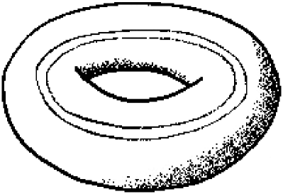
Figure 7. An open solid torus with a coaxial smaller closed solid torus removed is not weakly–Helmholtz.

The following lemma shows that, if $\partial\Omega$ is connected, then Lemma 5.24 does not provide any effective obstruction to be weakly–Helmhlotz.

Lemma 5.26.

If the boundary $\partial\Omega=S_{0}$ is connected, then ${\rm Ker}(i_{*})\subset H_{1}(S_{0})$ is a maximal Lagrangian submodule of $H_{1}(S_{0})$.

Proof. Lemma 5.6 implies that ${\rm Ker}(i_{\ast})$ is a direct summand of $H_{1}(S_{0})$ with ${\rm rank}\,{\rm Ker}(i_{*})=g(S_{0})=\frac{{\rm rank}\,H_{1}(S_{0})}{2}$, so it is enough to show that ${\rm Ker}(i_{\ast})$ is Lagrangian.

So let $\alpha$ be a $1$–cycle in ${\rm Ker}(i_{\ast})$ represented by a smooth loop $C_{1}\subset S_{0}$. If $[\beta]$ is any class in ${\rm Ker}(i_{\ast})={\rm Im}\,\partial$, then $[\beta]=\partial[\Sigma]$, where $\Sigma$ is a properly embedded surface in $(\overline{\Omega},\partial\Omega)$. Since $S_{0}$ admits a collar in $\overline{\Omega}$, we can push $\alpha$ a bit inside $\Omega$ and obtain a $1$–cycle $\alpha^{\prime}$ transverse to $\Sigma$. Since $[\alpha^{\prime}]=i_{\ast}([\alpha])=0$, the algebraic intersection between $\alpha^{\prime}$ and $\Sigma$ is null, and this easily implies in turn that $\langle[\alpha],[\beta]\rangle=0$, whence the conclusion. $\Box$

5.6. Weakly–Helmholtz links

We have seen in Corollary 5.22 that all knots and all the box–domains of knots are weakly–Helmholtz. On the other hand, if $L$ is the Hopf link (see Figure 8 below, on the left), then $\mathsf{C}(L)$ is diffeomorphic to an open tubular neighbourhood of the standard torus in ${\mathbb{R}}^{3}$, so $\mathsf{C}(L)$ is not weakly–Helmholtz (see Example 5.25). The same is true for $\mathsf{B}(L)$ (see Lemma 5.21). Lemma 5.27 below generalizes this result to a large class of links. We say that two components $K_{1}$ and $K_{2}$ of $L$ are algebraically unlinked if $K_{1}$ is homologically trivial in $\mathsf{C}(K_{2})$. It turns out that $[K_{1}]=0$ in $H_{1}(\mathsf{C}(K_{2}))$ if and only if $[K_{2}]=0$ in $H_{1}(\mathsf{C}(K_{1}))$, so the definition just given is indeed symmetric in $K_{1}$ and $K_{2}$. Equivalently, $K_{1}$ and $K_{2}$ are algebraically unlinked if and only if their linking number vanishes; moreover the linking number can be easily computed by using any planar link diagram as half the sum of the signs at the crossing points betweem the two components (for all this matter see e.g. [61] Section D of Chapter 5). Clearly, if two components of $L$ are geometrically unlinked (see Subsection 2.3), a fortiori they are also algebraically unlinked. The Whitehead link (see Figure 3 above on the left) is a celebrated example with two components that are algebraically, but not geometrically, unlinked. The components $K_{1}$ and $K_{2}$ are said to be algebraically linked it they are not algebraically unlinked. Evidently, the Hopf link has algebraically linked components.

Lemma 5.27.

If $L$ has algebraically linked components, then it is not weakly–Helmholtz.

Proof. Take two algebraically linked components $C_{0}$ and $C_{1}$ of $L$ and let $F_{0}$ be an oriented Seifert surface for $C_{0}$. As usual, we can assume that $F_{0}$ is transverse to $C_{1}$ and to the corresponding toric boundary component $S_{1}$ of $\partial\mathsf{C}(L)=\partial U(L)$, where $\mathsf{C}(L)=S^{3}\setminus U(L)$. Then the class $[\alpha]=p_{1}(\partial[F_{0}\setminus{\rm Int}(U(L))])\in p_{1}({\rm Ker}(i_{\ast}))\subset H_{1}(S_{1})$ is represented by the oriented intersection between $F_{0}$ and $S_{1}$, which is given by a finite number of (possibly non–equioriented) copies of the meridian of $S_{1}$. Since $C_{0}$ and $C_{1}$ are linked, the class $[\alpha]$ is not null in $H_{1}(S_{1})$, and is therefore equal to a non–trivial multiple of the class represented by the meridian of $S_{1}$. On the other hand, also the class $[\beta]$ of the preferred longitude on $S_{1}$, determined by any Seifert surface of $C_{1}$, belongs to $p_{1}({\rm Ker}(i_{\ast}))$, and $\langle[\alpha],[\beta]\rangle\neq 0$, so Lemma 5.24 implies that $L$ is not weakly–Helmholtz. $\Box$

Remark 5.28.

Lemma 5.27 implies the Hopf link is not weakly–Helmholtz. Thanks to the Lemma 5.21, it follows that the box–domain of such a link, drawn in the Figure 8 (on the right), is not weakly–Helmholtz as well.

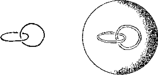
Figure 8. A box–domain of a Hopf link is not weakly–Helmholtz.

The following lemma considers the case of links with unlinked components.

Lemma 5.29.

Suppose that the components $C_{0},\ldots,C_{k}$ of a link $L$ are algebraically unlinked with each other. Then there exists a family of properly embedded surfaces $F_{0},\ldots,F_{k}$ such that each $F_{j}$ is a Seifert surface for $C_{j}$ and, if $i\neq j$, then $F_{i}$ and $F_{j}$ $($transversely$)$ intersect only in $\mathsf{C}(L)$. Moreover, if $i_{j}\colon S_{j}\longrightarrow\overline{\mathsf{C}(L)}$ is the inclusion of the boundary component corresponding to $C_{j}$ and $Q_{j}$ is the kernel of $(i_{j})_{\ast}\colon H_{1}(S_{j})\longrightarrow H_{1}(\overline{\mathsf{C}(L)})$, then $Q_{j}$ is generated by $($the class of$\,)$ the preferred longitude of $C_{j}$, and ${\rm Ker}(i_{*})=\bigoplus_{j}Q_{j}$.

Proof. Fix $j\in\{0,\ldots,k\}$ and take an arbitrary Seifert surface $F^{\prime}_{j}$ of $C_{j}$ transverse to every $C_{h}$, $h\neq j$. Up to re–defining $\mathsf{C}(L)$ as the complement in $S^{3}$ of smaller tubular neighbourhoods of the $C_{h}$’s, we may also assume that, for each fixed $h\neq j$, $F^{\prime}_{j}$ intersects transversely each $S_{h}$ in a finite number $m_{1},\ldots,m_{l}$ of (possibly non–equioriented) copies of the meridian of $S_{h}$, in such a way that each $m_{i}$ bounds a $2$–disk $D_{i}$ in the interior of $F^{\prime}_{j}$. Since the algebraic intersection of $C_{j}$ and $C_{h}$ is null, we also have $[m_{1}]+\ldots+[m_{l}]=0$ in $H_{1}(S_{h})$, so the number of positively oriented meridians occurring in the oriented intersection $F^{\prime}_{j}\cap S_{h}$ equals the number of negatively oriented meridians in the same intersection.

Let us now remove the $D_{i}$’s, $i=1,\ldots,l$, from the interior of $F^{\prime}_{j}$. In this way, we obtain a properly embedded surface with more boundary components. We can now glue in pairs the added boundary components by attaching $l/2$ disjoint annuli parallel to $S_{h}$ to $l/2$ pairs of meridians in $F^{\prime}_{j}\cap S_{h}$ having opposite orientations. After applying the procedure just described to every $h\neq j$, we obtain the desired Seifert surface $F_{j}$ that misses all the $S_{h}$, $h\neq j$.

Now, if $[l_{j}]\in H_{1}(S_{j})$ is the class of the preferred longitude of $C_{j}$, then $[l_{j}]=\partial[F_{j}]$, so $[l_{j}]$ lies in $Q_{j}$ and hence ${\rm rank}\,\bigoplus_{j}Q_{j}=k+1={\rm rank}\,{\rm Ker}(i_{\ast})$. Now the conclusion follows from the fact that $\bigoplus_{j}Q_{j}$ is a full submodule of $H_{1}(\partial\Omega)$. $\Box$

We may wonder if the Seifert surfaces of the previous lemma can be chosen to be pairwise disjoint. A classical definition is in order (see [61, p. 137]).

Definition 5.30.

A link $L$ is a boundary link if it admits a system of disjoint Seifert surfaces of its components.

Of course, every knot is a boundary link. Every link $L$ with geometrically unlinked components is a boundary link as well, as for every component $C$, we can construct a Seifert surface contained in the 3–disk that separates $C$ from the other components (see [61]). However, there are boundary links that have geometrically linked components. For example every 2–components links made by a non–trivial knot and its preferred longitude (recall Example 2.6) is a boundary link. On the left of Figure 10, we show the case of the trefoil knot, on the right another more complicated 3–components boundary link (see [61] for other examples). The meaning of the useful square–boxes labelled by any integer $k$ is fixed in Figure 9, where it is understood that the box contains $|k|$ crossings.

Figure 9. k–box.

Figure 10. Boundary links.

On the other hand, the Whitehead link provides an example of a link with algebraically unlinked components which is not a boundary link (see again [61, p. 137], and Example 5.34 below for an even stronger result). So, in general, it is not possible to remove the internal intersections of the Seifert surfaces provided by Lemma 5.29 by any local “cut and paste” procedure around the intersection lines.

Let us now rephrase Theorem 5.19 in the case of links.

Corollary 5.31.

A link $L$ with $r$ components is weakly–Helmholtz if and only if there is a surjective homomorphism from $\pi_{1}(\Omega(L))$ to ${\mathbb{Z}}^{\ast r}$.

We recognize that the condition described in the last corollary is just one current definition of homology boundary links, so a link is weakly–Helmholtz if and only if it is a homology boundary link. More precisely, putting together Corollary 5.31 and Lemma 5.21, we obtain the following:

Corollary 5.32.

Given a link $L$ in $S^{3}$, the following assertions are equivalent:

• $L$ is weakly–Helmholtz.

• $L$ is a homology boundary link.

• $\mathsf{B}(L)$ is weakly–Helmholtz.

Every classical boundary link is a homology boundary link. In fact, $L$ is a boundary link if and only if there exists a surjective homomorphism $\phi:\pi_{1}({\Omega(L)})\longrightarrow{\mathbb{Z}}^{\ast r}$, which furthermore (up to conjugacy) sends the link meridians onto a set of generators of ${\mathbb{Z}}^{\ast r}$. This characterization of boundary links was originally given in [67] (see also [40]), where also the relaxed definition of homology boundary links was introduced.

Homology boundary links are an intriguing, very important class of links widely studied in Knot Theory (the interested reader can find more It is a nice occurence that our discussion originated from Helmholtz cuts, eventually leads to such a distinguished class of links.

5.7. On general weakly–Helmholtz domains

Getting an exhaustive description of weakly–Helmholtz domains, similar to the characterization of Helmholtz ones given in Theorem 4.5, looks somehow hopeless. This already holds true for the special case of links. Note that concretely given a link $L$ (for instance by means of a usual planar link diagram), with algebraically unlinked components, it is in general a quite hard task to decide whether or not it is homology boundary (for example, some non–trivial argument is needed even for showing that the Whitehead link is not weakly–Helmholtz – see the examples below). The general case is even more complicated. Up to “Fox reimbedding” (see Theorem 4.9), it is not restrictive to deal with domains $\Omega$ that are the complements of links of handlebodies considered up to isotopy. As every handlebody is the regular neighbourhood of a spine, which is a compact graph embedded in $S^{3}$ (i.e. a spatial graph), if $\Gamma$ is a link of spines, then we can naturally extend our previous notation and denote by $\mathsf{C}(\Gamma)$ the complement–domain of $\Gamma$. In the case of a classical link $L$, i.e. in the case of a link of genus 1 handlebodies, we have in some sense a “canonical” spine for $\mathsf{C}(L)$: the link $L$ itself. This is no longer true in the general case, in the sense that a link of handlebodies, considered up to isotopy, can admit essentially different links of spines. This represents a further complication in the study of general weakly–Helmholtz domains.

To illustrate the last claim, we will consider the simplest case of just one genus 2 handlebody $\overline{H}$. Every such handlebody admits a spine $\Gamma$, which is a spatial embedding of the so–called “handcuff graph” (a planar realization of which is shown in Figure 11).

Figure 11. Planar handcuff graph.

If we remove from $\Gamma$ the interior of the edge that connects the two cycles (i.e. the “isthmus” of $\Gamma$), then we get a classical link $L_{\Gamma}$ with two components. Set $\Omega=\mathsf{C}(\Gamma)$ and $\Omega^{\prime}=\mathsf{C}(L_{\Gamma})$. Clearly $\overline{\Omega}\subset\overline{\Omega^{\prime}}$, as the first is obtained by removing a 1–handle from the second.

The following proposition will allow to contruct many examples of both non–homology boundary links with two algebraically unlinked components, and knotted genus 2 handlebodies having weakly–Helmholtz complementary domain.

Proposition 5.33.

With the notations just introduced, the following results hold:

1. If $L_{\Gamma}$ is a homology boundary link, then $\Omega$ is weakly–Helmholtz.

2. Suppose that $\overline{H}$ is unknotted. Then $L_{\Gamma}$ is a homology boundary link if and only if $\Gamma$ is planar. In particular, if $L_{\Gamma}$ is non–trivial, then it is not a homology boundary link.

Proof. By a general position argument, it is easy to see that every loop in $S^{3}\setminus L_{\Gamma}$ is homotopic to a loop that does not intersect the isthmus of $\Gamma$. This implies that $i_{*}:\pi_{1}(\overline{\Omega})\to\pi_{1}(\overline{\Omega^{\prime}})$ is surjective. Then (1) follows immediately from Theorem 5.19 and Corollary 5.31.

Let us now suppose that $\overline{H}$ is unknotted. Then also $\overline{\Omega}$ is an unknotted genus 2 handlebody, hence $\pi_{1}(\overline{\Omega})\cong{\mathbb{Z}}^{*2}$, and $\pi_{1}(\overline{\Omega^{\prime}})$ is isomorphic to a quotient of $\pi_{1}(\overline{\Omega})$. Therefore, if $L_{\Gamma}$ is homology boundary, then we have a sequence of surjective homomorphisms

$${\mathbb{Z}}^{*2}\cong\pi_{1}(\overline{\Omega})\to\pi_{1}(\overline{\Omega^{\prime}})\to{\mathbb{Z}}^{*2}\ .$$

But free groups are Hopfian (see [52]), which means that every surjective homomorphism of ${\mathbb{Z}}^{*2}$ onto itself is in fact an isomorphism, and this implies here that $\pi_{1}(\Omega^{\prime})$ is isomorphic to ${\mathbb{Z}}^{*2}$. Under this hypothesis, a generalization to links (see for instance Theorem 1.1 in [45]) of Papakyriakopoulos unknotting theorem for knots [59] (which is based on his famous “loop theorem” – see also [61]) ensures that $L_{\Gamma}$ is trivial, and we can finally apply the planarity results of [64] and conclude that $\Gamma$ is planar. $\Box$

We stress that $\overline{H}$ may admit infinitely many handcuff spines with pairwise non–isotopic associated links (see the examples below). Hence, if $\Omega$ is not weakly–Helmholtz, point (1) of the above proposition implies that no such link is homology boundary. However, checking whether this last condition is satisfied seems to be very demanding.

Example 5.34.

(1) In Figures 12 and 13, we show some spatial handcuff graphs $\Gamma$ that become planar via a finite sequence of spine modifications that keep the handlebody $\overline{H}$ fixed up to isotopy. In Figure 13, it is understood that $h=(-1)^{k}2$.

Figure 12. Unplanar vs planar handcuff spines.

Figure 13. More unplanar vs planar handcuff spines.

The fact that the spines described here can be modified into planar graphs shows that, in every case, $\overline{H}$ is unknotted, so, by point (2) of Proposition 5.33, we see that all the corresponding non–trivial links $L_{\Gamma}$ are not homology boundary. The first example deals once again with the Hopf link by showing also the somewhat non–intuitive phenomenon that being $L_{\Gamma}$ geometrically linked does not prevent $\overline{H}$ to be unknotted. The second example establishes that eventually the Whitehead link is not homology boundary. The examples described in Figure 13 provide an infinite family of links (with the exceptions of $k=0,1$ that produce the trivial link) having algebraically unlinked components that are not homology boundary. Note that every link in the family has one unknotted component, while the other component is equal to the trefoil knot when $k=-1$, the figure–eight knot when $k=-2$, etc. Note that when $k=2$ we get Whitehead link again.

(2) If $L_{\Gamma}$ has geometrically unlinked components (i.e. if it is a split–link), then $\Omega=\mathsf{C}(\Gamma)$ is weakly–Helmholtz by point (1) of Proposition 5.33. If we assume furthermore that $L_{\Gamma}$ is non–trivial, then $\overline{H}$ is knotted by point (2). Remarkably, there exists also an example where $\overline{H}$ is knotted whereas $L_{\Gamma}$ is trivial. In fact, it is proved in [50] that the handlebody $\overline{H}$ determined by the spine $\Gamma$ of Figure 14 is knotted.

Figure 14. Knotted handlebody vs weakly–Helmholtz domain.

Proposition 5.33 does not suggest how to construct examples of domains with connected boundary of genus 2 which are not weakly–Helmholtz. In fact we conclude our discussion with the following open problem (as far as we know):

Question 5.35.

Construct (if any) a knotted handlebody of genus 2 whose complement–domain is not weakly–Helmholtz. Same question with arbitrary genus. Due to Fox reimbedding Theorem, such handlebodies exist if and only if there exist domains with connected locally flat boundary, which are not weakly–Helmholtz.

5.8. Appendix

Without any pretension of being exhaustive, in this appendix we will indicate to the interested reader some more advanced topics related to the previous discussion.

Let ${\mathcal{L}}$ be a link of spines and suppose we are given a concrete presentation of ${\mathcal{L}}$ (for instance by means of planar diagrams associated to generic planar projections). Then it is rather easy to produce finite presentations of the fundamental group of $S^{3}\setminus{\mathcal{L}}$ (such as the Wirtinger presentation – see [61]). Fox’s free differential calculus [35] is a fundamental tool for the study of groups defined by generators and relations. However, determining the corank starting from a finite presentation of a group is in general a quite hard task. In [68], either this is done for certain presentations with particular formal properties, or one gives equivalent topological 3–dimensional reformulations, very close, in our framework, to the spirit of Theorem 5.19.

In the case of classical links, we may recur to certain, in principle computable, increasingly discriminating sequence of invariants (“obstructions”) whose vanishing is a necessary condition in order to be homology boundary (at the initial step we have just the obstruction given by the linking numbers of pairs of link components, discussed in Lemma 5.27). The original definition of such invariants is given in [57], so that they are known as Milnor’s $\bar{\mu}$ invariants. Let us recall some of their formal features. For every integer $q>1$, for every link $L$ with $N$ ordered and oriented components $K_{1},\dots,K_{N}$, for every $(l_{1},\dots,l_{p})\in{\mathbb{N}}^{p}$, with $1\leq l_{i}\leq N$, $p<q$, it is defined an invariant of the form

$$\bar{\mu}(l_{1},\dots,l_{p})(L)=[\mu(l_{1},\dots,l_{p})(L)]\in{\mathbb{Z}}/\Delta(l_{1},\dots,l_{p}){\mathbb{Z}}$$

where:

- the integer $l_{j}$ is intended as a label of the component $K_{l_{j}}$ (note that any index $l_{j}$ can be repeated);

- the integer $\mu(l_{1},\dots,l_{p})(L)$ is (not uniquely) obtained by means of a determined procedure;

- the integer $\Delta(l_{1},\dots,l_{p})$ is defined inductively as the g.c.d. of the numbers $\mu(j_{1},\dots,j_{s})(L)$ where $s\geq 2$ and $(j_{1},\dots,j_{s})$ ranges over all cyclic permutations of proper subsequences of $(l_{1},\dots,l_{p})$.

- if $j_{1}\neq j_{2}$, the value $\mu(j_{1},j_{2})(L)$ is the linking number of the corresponding components.

Strictly speaking, Milnor’s invariants are isotopy invariants for ordered and oriented links. However, their vanishing does not depend on the chosen order or orientation. The actual definition has a strong algebraic flavour, by dealing with presentations of the fundamental group $G_{1}:=\pi_{1}(\mathsf{C}(L))$. Roughly speaking, Milnor’s invariants detect whether or not the (preferred) longitudes of the link components can be expressed as longer and longer commutators (i.e. they detect how deep the longitudes live in the lower central series of the link group, which is inductively defined as follows: $G_{1}=\pi_{1}(\mathsf{C}(L))$, and $G_{n}=[G_{n-1},G_{1}]$ is the subgroup of $G$ generated by the set $\{aba^{-1}b^{-1}\ ;\ a\in G_{n-1},\ b\in G_{1}\ \}$. The invariants relative to a given $q$ as above represent obstructions to the fact that the longitudes belong to $G_{q}$).

In [60] and [70], it is established an equivalent definition of Milnor’s invariants in terms of the Massey products in the systems $\{S^{3}\setminus K_{l_{j}}\}_{j=1}^{p}$. This approach provides an increasingly discriminating sequence of algebraic–topological obstructions defined by means of the cup product on singular 1–cochains with coefficients in ${\mathbb{Z}}/\Delta(l_{1},\dots,l_{p}){\mathbb{Z}}$, and the coboundary operator.

In [28], one can find a more geometric approach to these invariants, based on the construction of so–called “derived links”. This method is particularly suited in order to deal with the “first non–vanishing” invariant (if any). In a sense it is a geometric realization of the Massey products, working with relative 2–cycles rather than 1–cochains, and replacing the cup product with the transverse intersection of such 2–cycles. The naive idea of a derived link is as follows. Consider a link $L$ as in Lemma 5.29, then we can construct a system of Seifert surfaces intersecting transversely only in $\mathsf{C}(L)$. We can manage in order that the intersection of each couple of surfaces is one connected knot in $\mathsf{C}(L)$. Each such knot splits in two parallel copies by slightly isotoping it out of both surfaces, by using the respective collars in the positive normal direction (accordingly to the orientations). By taking all knots obtained in this way, we get a derived link $L^{\prime}$ of the given link $L$. We can define “higher order” invariants of $L$ by using the linking numbers of the pairs of components of $L^{\prime}$. If all these linking numbers vanish, we iterate the procedure.

In [28] and [60], one finds some examples of computations of non–trivial Milnor’s invariants. In particular, when $L$ is the Whitehead link, we see that $\bar{\mu}(1,1,2,2)(L)=1$, accordingly to the fact that $L$ is not homology boundary.

Milnor’s invariants with pairwise distinct indices $l_{j}$ have a particular meaning. In fact, they are invariant up to link homotopy equivalence (also introduced in [57]). This means that one allows homotopy with self–crossings of each link component, while crossings of different components are not allowed. If a link $L$ is link homotopy equivalent to a trivial link, then all such special Milnor’s invariants vanish. Note, for example, that the Whitehead link becomes trivial just by performing one self–crossing at one component (see Figure 3). In [27] or [32], it is proved that every boundary link is link homotopic to a trivial link. The link–homotopy classification was given in [57] for 2– and 3–components links, in [51] for 4–components ones; finally for all links in [41]. General Milnor’s invariants are invariants up to link concordance equivalence. Homology boundary links have been widely studied in this framework [28, 29, 30, 31, 26].

The theory of links of spatial graphs as well as of links of handlebodies is considerably less developed than the classical link theory. Links of spatial graphs have been more intensively considered, by extending to them different equivalence relations (“homotopy”, “cobordism”, “homology”,…) [33, 69, 66]. Particular efforts have been dedicated to detect whether or not a link is planar (up to isotopy) [63, 72]. A largely diffused approach consists in associating to every link of spatial graphs some invariant families of classical links [47, 48, 39], in order to exploit such a more developed theory.

The theory of links of handlebodies is even less developed. A natural approach consists in considering links of spines, that is links of spatial graphs up to isotopy coupled with suitable spine modifications that do not alter the carried handlebodies [64, 49, 50].

Note on the bibliography. References [1] to [18] form the “Section A” relative to Electromagnetism, Hydrodynamics and Elasticity on domains in ${\mathbb{R}}^{3}$. References [19] to [72] form the “Section B” on (3–dimensional) Differential/Algebraic/Geometric Topology.

References

- [1] C. Amrouche, C. Bernardi, M. Dauge and V. Girault, “Vector potentials in three-dimensional non–smooth domains,” Math. Methods Appl. Sci. 21 (1998) no. 9, 823–864.
- [2] A. Alonso Rodríguez, P. Fernandes and A. Valli, “The time–harmonic eddy–current problem in general domains: solvability via scalar potentials,” Computational electromagnetics (Kiel, 2001), 143–163, Lect. Notes Comput. Sci. Eng. 28, Springer, Berlin, (2003).
- [3] A. Bermúdez, R. Rodríguez P. Salgado, “A finite element method with Lagrange multipliers for low-frequency harmonic Maxwell equations”, SIAM J. Numer. Anal. 40 (2002), no. 5, 1823–1849.
- [4] A. Bossavit, “Computational electromagnetism”, Variational formulations, complementarity, edge elements. Electromagnetism, Academic Press, Inc., San Diego, CA, (1998).
- [5] A. Bossavit, A. Vourdas and K. J. Binns, “Magnetostatics with scalar potentials in multiply connected regions”, IEE Proc. A 136 (1989) no. 5, 260–261.
- [6] J. Cantarella, D. De Turck, H. Gluck, “Vector calculus and the Topology of Domains in 3-Spaces”, The American Mathematical Monthly, Vol. 109, No. 5, (May, 2002), 409–442.
- [7] R. Dautray, J.–L. Lions, “Mathematical analysis and numerical methods for science and technology. Vol. 3. Spectral theory and applications. With the collaboration of Michel Artola and Michel Cessenat. Translated from the French by John C. Amson”, Springer–Verlag, Berlin, (1990).
- [8] P. Fernandes, G. Gilardi, “Magnetostatic and electrostatic problems in inhomogeneous anisotropic media with irregular boundary and mixed boundary conditions”, Math. Models Methods Appl. Sci. 7 (1997) no. 7, 957–991.
- [9] C. Foias, R. Temam, “Remarques sur les équations de Navier–Stokes stationnaires et les phénomènes successifs de bifurcation,” Ann. Scuola Norm. Sup. Pisa Cl. Sci. (4) 5 (1978) no. 1, 28–63.
- [10] G. Geymonat, F. Krasucki, “Hodge decomposition for symmetric matrix fields and the elasticity complex in Lipschitz domains,” Commun. Pure Appl. Anal 8 (2009) no. 1, 295–309.
- [11] R. Ghiloni, “The Hodge decomposition theorem for general three–dimensional vector fields, without cuts”, to appear.
- [12] P. W. Gross, P. R. Kotiuga, “Electromagnetic theory and computation: a topological approach,” Mathematical Sciences Research Institute Publications 48, Cambridge University Press, Cambridge, (2004).
- [13] L. Kettunen, K. Forsman and A. Bossavit, “Formulation of the eddy current problem in multiply connected regions in terms of ”, Internat. J. Numer. Methods Engrg. 41 (1998) no. 5, 935–954.
- [14] L. Kettunen, K. Forsman and A. Bossavit, “Discrete Spaces for Div and Curl–Free Fields,” IEEE Transactions on Magnetics 34 (1998) no. 5, 2551–2554.
- [15] P. R. Kotiuga, “On Making Cuts for Magnetic Scalar Potentials in Multiply Connected regions”, Journal of Applied Physics 61(8) (1987), 3916–3918.
- [16] P. R. Kotiuga, A. Vourdas and K. J. Binns, “Correspondence on Magnetostatics with scalar potentials in multiply connected regions”, IEE Proc. A 137 (1990) no. 4, 231–232.
- [17] D. Mitrea, M. Mitrea and M. Taylor, “Layer potentials, the Hodge Laplacian, and global boundary problems in nonsmooth Riemannian manifolds”, Mem. Amer. Math. Soc. 150 (2001), no. 713.
- [18] R. Temam, “Navier–Stokes equations. Theory and numerical analysis. With an appendix by F. Thomasset. Third edition,” Studies in Mathematics and its Applications, 2, North–Holland Publishing Co., Amsterdam, (1984). *******
- [19] J.W. Alexander, “An example of a simply-connected surface bounding a region which is not simply–connected”, Proc. Nat. Acad. Sci. 10, 8–10, 1924.
- [20] J.W. Alexander, “On the subdivision of 3–space by a polyhedron”, Proc. Nat. Acad. Sci. 10, 6–8, 1924.
- [21] J.W. Alexander, “Remarks on a point set constructed by Antoine”, Proc. Nat. Acad. Sci. 10, 10–12, 1924.
- [22] R. H. Bing, “Locally tame sets are tame”, Ann. of Math. (2) 59 (1954) 145–158.
- [23] K. Borsuk, “Über die Fundamentalgruppe der Polyeder im euklidischen dreidimensionalen Raume”, Monatshefte für Math. u. Physik 41 (1934), 64–77.
- [24] R. Bott, L. Tu, “Differential forms in algebraic topology”, Springer, 1982.
- [25] M. Brown, “Locally flat imbeddings of topological manifolds”, Ann. of Math. (2) 75 (1962), 331–341.
- [26] A. Casson, ”Link cobordism and and Milnor’s invariants”, Bull. London Math. Soc. 7, 1975, 39–40.
- [27] L. Cervantes, R.A. Fenn, ”Boundary links are homotopy trivial”, Quart. J. Math. Oxford Ser. (2) 39, 1988, 151–158.
- [28] T. Cochran, “Derivatives of links: Milnor’s concordance invariants and Massey products”, Memoirs of the A.M.S. Vol. 84, N. 427, 1990.
- [29] T. Cochran, J. Levine, “Homolopy boundary links and the Andrews Curtis conjecture”, Topology, 30, 1991, 231–240.
- [30] T. Cochran, K,E. Orr, “Not all links are concordant to boundary links”, Annals of Math., 1993.
- [31] T. Cochran, K,E. Orr, “Homology Boundary Links and Blanchfield Forms: Concordance Classsification and New Tangle-Theoretic Constructions”, Topology 1994.
- [32] D. Dimovski, ”A geometric proof that boundary links are homotopically trivial”, Topology Appl. 29, 1988, 237–244.
- [33] T. Fleming, R. Nikkuni, ”Homotopy on spatial graphs and the Sato-Levine invariant”, Trans. Amer. Math. Soc. Vol. 361, N. 4, 2009, 1885–1902.
- [34] R.H. Fox, “On the Imbedding of Polyhedra in 3-Space”, Annals of Mathematics, Second Series, Vol. 49, No.2 (Apr. 1948), 462–470.
- [35] R.H. Fox, ”Free differential Calculus”, Ann. of Math. Vol. 57, N. 3, 1953, 547-560.
- [36] C.McA. Gordon, “3–dimensional topology up to 1960”, in “History of Topology”, Ed. I.M. James, North-Holland, Elsevier, 1999.
- [37] M. J. Greenberg, “Lectures on algebraic topology”, W. A. Benjamin, Inc., New York–Amsterdam, (1967).
- [38] L. Guillou, A. Marin, “A la recherche de la Topologie Perdue”,Progress in Mathematics, Vol. 62, Birkhäuser, 1986.
- [39] S.M. Ghuman, ”Seifert surfaces for graphs”, Journal of Knot Theory and its Ramifications, Vol. 8, N. 8 1999, 985–999.
- [40] M.A. Gutierrez, “Boundary links and an unlinking theorem”, Trans. Amer. Math. Soc., 17, 1972, 491–499.
- [41] N. Habegger, X.S. Lin, ” The classification of links up to link homotopy”, J. Amer. Math. Soc. 3, 1990, 389-419.
- [42] S. Harvey, “On the cut number of a –manifold”, Geom. Topol. 6 (2002), 409–424.
- [43] A. Hatcher, “Algebraic Topology”, Cambridge University Press, 2002, (Single electronic copy freely available from http://www.math.cornell.edu/ hatcher/).
- [44] A. Hatcher, “Basic 3-Manifold Topology”, http://www.math.cornell.edu/ hatcher/3M/3Mdownloads.html
- [45] J.A. Hillman, ”Algebraic invariants of links”, Series on Knots and Everything, Vol. 32, World Scientific, Singapore (2002).
- [46] M.W. Hirsch, “Differential Topology”, Graduate Texts in Mathematics Vol. 33, Springer-Verlag, New York (1994).
- [47] L.H. Kauffman, ”Invariants of Graphs in 3-space”, Transactions of the Amer. Math. Soc. Vol. 311, N.2, 1989, 697-710.
- [48] L.H. Kauffman, J. Simon, K. Wolcott, P. Zhao, ”Invariants of theta-curves and other graphs in 3-space”, Topology and its Applications, 49, 1993, 193–216.
- [49] A. Ishii, ”Moves and invariants for knotted handlebodies”, Algebraic and Geometric Topology 8, 2008, 1403-1418.
- [50] A. Ishii, M. Iwakiri, ” Quandle cocycle invariants for spatial graphs and knotted handlebodies”, arXiv, preprint 2008.
- [51] J.P. Levine, ” An approach to homotopy classification of links”, Trans. Amer. Math. Soc. 306, 1988, 361–387.
- [52] W. Magnus, A. Karras, B. Solitar, ” Combinatorial group theory: presentations in terms of generators and relators”, Wiley (Interscience) 1966.
- [53] W. S. Massey, “Algebraic topology: An introduction,” Harcourt, Brace & World, Inc., New York, (1967).
- [54] J.W. Milnor, “Morse Theory”, Annals Studies 51, Princeton Univ. Press, 1963.
- [55] J.W Milnor, “Lectures on the h-cobordism theorem”, notes by L. Siebenmann and J. Sondow, Princeton University Press, Princeton, NJ 1965.
- [56] J.W. Milnor, “Topology from the differentiable viewpoint”, The University Press of Virginia, 1969.
- [57] J.W. Milnor, “Link Groups”, Annals of Math., Vol. 59, N.2 (March 1954), 177–195.
- [58] E.E. Moise, “Geometric Topology in Dimensions 2 and 3”, Springer-Verlag, 1977.
- [59] C.D. Papakyriakopoulous, ”On Dehn’s lemma and the asphericity of knots”, Ann.of Math. (2), 1957, 1-26.
- [60] R. Porter, “Milnor’s invariants and Massey products”, Trans. Amer. Math. Soc. 257, 30–71, 1980.
- [61] D. Rolfsen, “Knots and links”, Mathematics Lecture Series, 7, Publish or Perish, Inc., Berkeley, Calif., (1976).
- [62] C.P. Rourke, B.J. Sanderson, “Introduction to piecewise-linear topology”, Springer, 1972.
- [63] M.Scharlemann, A. Thompson, ” Detecting unknotted graphs in 3-spaces”, J. Differential Geometry, 34, 1991, 539-560.
- [64] M.Scharlemann, A. Thompson, ” Thin position and Heegaard splittings of the 3-sphere”, J. Differential Geometry, 39, 1994, 343-357.
- [65] A.S. Sikora, “Cut numbers of –manifolds”, Trans. Amer. Math. Soc., 357 (2004), 2007–2020.
- [66] R. Shinjo, K. Taniyama, ”Homology classification of spatial graphs by linking numbers and Simon invariants”, Topology Appl. 134, 2003, N. 1, 53–67.
- [67] N. Smythe, “Boundary links”, in Topology Seminars, Ann. Math. Studies 60, ed. R.H. Bing, Princeton Univ. Press 1965.
- [68] J.R. Stallings, “Problems about free quotients of groups”, Geometric group theory (Columbus, OH, 1992), 165-182, Ohio State Univ. Math. Res. Inst. Publ. 3, de Gruyter, Berline, 1995.
- [69] K. Taniyama, ”Cobordism, homotopy and homology of graphs in ”, Topology, 33, 1994, 509–523.
- [70] V.G. Turaev, “The Milnor invariants and Massey products”, in Studies in Topology II, Acad. Nauk USSR 66 (1976), in translation Journ. Soviet Math.
- [71] F. Waldhausen, “Heegaard-Zerlegungen der 3-Sphäre”, Topology 7 (1968), 195–203.
- [72] P. Zhao, ” Is a knotted graph determined by its associated links?”, Topology and its Applications, 57, 1994, 23–30.