Synchronized chaos in networks of simple units

Abstract

We study synchronization of non-diffusively coupled map networks with arbitrary network topologies, where the connections between different units are, in general, not symmetric and can carry both positive and negative weights. We show that, in contrast to diffusively coupled networks, the synchronous behavior of a non-diffusively coupled network can be dramatically different from the behavior of its constituent units. In particular, we show that chaos can emerge as synchronized behavior although the dynamics of individual units are very simple. Conversely, individually chaotic units can display simple behavior when the network synchronizes. We give a synchronization criterion that depends on the spectrum of the generalized graph Laplacian, as well as the dynamical properties of the individual units and the interaction function. This general result will be applied to coupled systems of tent and logistic maps and to two models of neuronal dynamics. Our approach yields an analytical understanding of how simple model neurons can produce complex collective behavior through the coordination of their actions.

I Introduction

Dynamical processes in networks, such as synchronization, have been attracting much interest Pikovsky-book ; Boccaletti02 ; Arenas08 ; Chavez07 . A striking characteristic of many networks is that they are often formed from very simple units (e.g. a neuron either spikes or is silent, at a certain level of description) but can collectively exhibit a wide range of dynamics. A central question is then how dynamically simple units can produce rich collective dynamical behavior when they are coupled together in a network. In this letter we offer a solution to this question in the context of synchronization of coupled map networks.

Previous work on synchronization of coupled maps focused on diffusive coupling with non-negative weights. However, in diffusively-coupled networks the synchronized network shows the same dynamical behavior as one single isolated unit; thus, no new collective behavior is emerging here. New collective behavior could, for instance, be produced by time delays, which may remarkably make it easier for networks to synchronize Atay04b ; Atay06 .

Here however, instead of time delays, we consider non-diffusive coupling schemes. One particular non-diffusive coupling scheme, the so-called direct coupling scheme is motivated by biological findings (see Dayan01 and the references therein) and has been used in studies of amplitude response of coupled oscillators Aronson90 , although not investigated as extensively as diffusive coupling in synchronization research. In this letter, we use a direct coupling scheme to study the emergence of new collective dynamical behavior. In particular, we show the emergence of synchronized chaotic behavior in a network of non-chaotic units. To our knowledge this is the first time that such a phenomenon is observed and analyzed in depth in mathematical network models. In contrast, synchronized chaotic behavior in a network of chaotic units Pecora90 ; Kaneko90 and non-synchronized chaotic behavior in a network of non-chaotic units Li04 are well established phenomena.

A further feature of this work is that we take the succeeding, typically in the literature neglected, facts into account. Many biological networks share the following two properties Dayan01 : $(i)$ The connection structure is, in general, not symmetric. $(ii)$ The influence of neighboring units can be excitatory or inhibitory, which is modelled by positive and negative weights. It is thus essential to incorporate these characteristics in network models in order to understand the dynamical behavior of biological networks. Consequently, we consider networks with arbitrary network topologies, namely, not necessarily symmetrically coupled networks with possibly both positive and negative weights. On the other hand, we restrict ourselves to networks of identical units. We mention, e.g., Sun09 , as a recent study of diffusively-coupled units with small parametric variations.

In order to emphasize a general aspect, we consider in the next section networks with pairwise coupling and present a general synchronization criterion. Later on, we will focus on directly coupled networks and study the emergence of new behavior.

II Pairwise coupling

In our coupled map network model, each node is a dynamical system whose evolution is described in discrete time $t$ by iterations of a scalar map $f$, i.e. by an equation of the form

$$x(t+1)=f(x(t)).$$ (1)

The interconnections are specified by a weighted, directed graph $\Gamma$ on $n$ vertices. The weight $w_{ij}$ of the connection from vertex $j$ to vertex $i$ can be positive, negative or zero. We assume that the network has no self-loops, that is, $w_{ii}=0$ for all $i$. The in-degree of vertex $i$ is $d_{i}=\sum_{j=1}^{n}w_{ij}$ . The activity at vertex or unit $i$ at time $t+1$ is given by:

$$x_{i}(t+1) = f(x_{i}(t))+\frac{\epsilon}{d_{i}}\sum_{j=1}^{n}w_{ij}g(x_{i}(t),x_{j}(t)),$$

$$\qquad\qquad\qquad\qquad\qquad\,i=1,...,n,$$

where $f:\mathbb{R}\rightarrow\mathbb{R}$ and $g:\mathbb{R}^{2}\rightarrow\mathbb{R}$ are differentiable functions with bounded derivatives, and $\epsilon\in\mathbb{R}$ is the overall coupling strength. The function $f$ describes the dynamical behavior of the individual units whereas $g$ characterizes the interactions between different pairs of units.

III Synchronization

We are interested in synchronized solutions of eq. (II), where the activity of all units is identical, that is, $x_{i}(t)=s(t)$ for all $i$ and $t$. It follows from eq. (II) that a synchronized solution $s(t)$ satisfies

$$s(t+1)=f(s(t))+\epsilon g(s(t),s(t)).$$ (3)

This equation already shows that the synchronized solution $s(t)$ can be quite different from the dynamical behavior of an isolated unit described by $f$. By contrast, in diffusive-type coupling, i.e. $g(x,x)=0$ for all $x$, the interaction $g$ vanishes when the network is synchronized; therefore, the synchronized solution is identical to the behavior of the individual units, and no new dynamics can emerge from synchronization.

Before we explore different examples of new collective behavior, we investigate the robustness of the synchronized state against perturbations. The network is said to (locally) synchronize if $\lim_{t\rightarrow\infty}|x_{i}(t)-x_{j}(t)|=0$ for all $i,j$ starting from initial conditions in some appropriate open set. The propensity of the network to synchronize depends on the properties of the functions $f$ and $g$ and the underlying network structure. The latter can be encoded in terms of the eigenvalues of the graph Laplacian $\mathcal{L}$ for directed weighted graphs, defined as Bauer08

$$(\mathcal{L})_{ij}:=\left\{\begin{array}[]{r cl}1&&\,\mbox{ if}\;i=j\mbox{ and $d_{i}\neq 0$}.\\ -\frac{w_{ij}}{d_{i}}&&\begin{array}[]{l}\mbox{if there is a directed edge }\\ \mbox{from $j$ to $i$ and $d_{i}\neq 0$.}\end{array}\\ 0&&\,\mbox{ otherwise.}\end{array}\right.$$ (4)

We label the eigenvalues of $\mathbf{\mathcal{L}}$ as $\lambda_{1},...,\lambda_{n}$. Since we assume that the in-degrees are non-zero, we may write $\mathcal{L}=I-D^{-1}W,$ where $I$ is the ($n\times n$) identity matrix, $D=\mathrm{diag}\{d_{1},...,d_{n}\}$ is the diagonal matrix of vertex in-degrees and $W=\left(w_{ij}\right)_{i,j=1}^{n}$ is the weighted adjacency matrix of the underlying graph. Zero is always an eigenvalue of $\mathcal{L}$; we denote it $\lambda_{1}=0$, and $u_{1}=(1,\ldots,1)^{\top}$ is the corresponding eigenvector.

Since all components of $u_{1}$ are identical, perturbations along the $u_{1}$-direction again yield a synchronous solution. To study the remaining directions, we define the k-th mixed transverse exponent $\chi_{k}$ for $2\leq k\leq n$ as:

$$\chi_{k}:=\overline{\lim}_{T\rightarrow\infty}\frac{1}{T}\sum_{s=\bar{t}}^{\bar{t}+T-1}\log|h_{k}(s(t))|,$$ (5)

where

$$h_{k}(s(t)) = f^{\prime}(s(t))+\epsilon\partial_{1}g(s(t),s(t))$$

$$+\epsilon\partial_{2}g(s(t),s(t))(1-\lambda_{k})$$

and $\partial_{i}g$ denotes the ith partial derivative of $g$ and $\bar{t}$ is chosen such that $h(s(t))\neq 0$ for all $t>\bar{t}$. If no such $\bar{t}$ exists we set $\chi_{k}=-\infty$. Note that these exponents are evaluated along the synchronous solution (3). They combine the dynamical behavior of the individual units and the interaction function with the network topology. The maximal mixed transverse exponent governs the synchronizability of the network, that is, system (II) locally synchronizes if

$$\chi:=\max_{k\geq 2}\chi_{k}<0.$$ (6)

This result is rigorously derived in our companion paper Bauer08b .

IV Diffusive and direct coupling

In the sequel, we restrict ourselves to functions $g:\mathbb{R}\rightarrow\mathbb{R}$. When $g(x_{i},x_{j})=g(x_{j})$, pairwise coupling reduces to direct coupling, i.e.,

$$x_{i}(t+1)=f(x_{i}(t))+\frac{\epsilon}{d_{i}}\sum_{j=1}^{n}w_{ij}g(x_{j}(t)),\;\;i=1,...,n$$ (7)

and the mixed transverse exponent (5) reduces to

$$\chi^{direct}_{k}:=\lim_{T\rightarrow\infty}\frac{1}{T}\sum_{s=\bar{t}}^{\bar{t}+T-1}\log|f^{\prime}(s(t))+\epsilon g^{\prime}(s(t))(1-\lambda_{k})|.$$ (8)

By rearranging terms on the right hand side in (7) as

$$f(x_{i}(t))+\epsilon g(x_{i}(t))+\frac{\epsilon}{d_{i}}\sum_{j=1}^{n}w_{ij}(g(x_{j}(t))-g(x_{i}(t))),$$ (9)

this becomes formally equivalent to a system of the form

$$x_{i}(t+1)=\phi(x_{i}(t))+\frac{\epsilon}{d_{i}}\sum_{j=1}^{n}w_{ij}\gamma(x_{j}(t),x_{i}(t)),$$ (10)

with $\gamma(x,x)=0$ for all $x$, i.e., a diffusively coupled map network. Thus, the conditions for synchronization of directly coupled networks (8) can be deduced from the diffusive coupling case (10) of Pecora98 . However, the formal equivalence obscures the roles of the system parameters and the particular coupling functions, which are important in applications. For instance, in neuronal networks, gap junctions at electrical synapses provide connections of diffusive type, whereas chemical synapses provide connections with direct coupling. The distinction is crucial for understanding the effects of different types of synapses. As already mentioned, diffusively-coupled networks have been widely studied. For the remainder of this work, we restrict ourselves to direct coupling.

The definition of $\chi^{direct}_{k}$ intertwines the effects of the resulting synchronized dynamics and the network topology. However, if $g$ is a multiple of $f$, i.e. $g=cf$ for some constant $c$, then these effects can be separated as the synchronization condition (6) takes the form

$$\max_{k\geq 2}\log\left|1-\frac{\epsilon c}{1+\epsilon c}\lambda_{k}\right|+\mu_{(1+\epsilon c)f}<0$$ (11)

where

$$\mu_{(1+\epsilon c)f}:=\overline{\lim}_{T\rightarrow\infty}\frac{1}{T}\sum_{s=\bar{t}}^{\bar{t}+T-1}\log|(1+\epsilon c)f^{\prime}(s(t))|$$ (12)

is the Lyapunov exponent of $(1+\epsilon c)f(x)$. Here $\bar{t}$ is chosen such that $f^{\prime}(s(t))\neq 0$ for all $t>\bar{t}$. In the sequel, let $\mathcal{D}(c,r)$ denote the disk in the complex plane centered at $c$ having radius $r$. It is easy to see that (11) is equivalent to the condition that all eigenvalues, except $\lambda_{1}$, are contained in $\mathcal{D}(c^{*},r^{*})$, where

$$c^{*}=\frac{1+\epsilon c}{\epsilon c}$$ (13)

and

$$r^{*}=\left|c^{*}\right|\exp(-\mu_{(1+\epsilon c)f}).$$ (14)

If, for example, the synchronized solution $(1+\epsilon c)f(x)$ is chaotic (i.e. has a positive Lyapunov exponent), then the first term in (11) has to be sufficiently negative to compensate the positive Lyapunov exponent in order to ensure that the system (7) locally synchronizes. This in turn requires that the eigenvalues $\lambda_{k}$ for $k\geq 2$ be bounded away from zero, and the coupling strength $\epsilon$ lie in an appropriate interval.

V Coupled tent maps

Before turning to biologically motivated functions $f$ and $g$, we demonstrate the emergence of synchronized chaotic behavior for the case of the tent map where an analytical treatment is possible. The tent map is given by

$$T_{\rho}(x)=\left\{\begin{array}[]{l c l}\rho x,&\mbox{if}&x<\frac{1}{2}\\ \rho(1-x),&\mbox{if}&x\geq\frac{1}{2},\end{array}\right.$$ (15)

for $\rho\in[0,2]$. Its Lyapunov exponent is $\log\rho$; thus, it is chaotic for $\rho>1$. Let $f(x)=T_{a}(x)$ and $g(x)=T_{b}(x)$ with $0<a,b<2$ and choose the coupling constant $\epsilon=(\tau-a)/b$. By choosing different values for the target value $\tau$ we can generate different synchronized dynamical behavior $s(t+1)=T_{\tau}(s(t))$ whose Lyapunov exponent equals $\log\tau$. Since the absolute value of the derivative of $T_{\tau}(x)$ is constant, from (11) we have that the system (7) locally synchronizes if

$$\left|\tau-(\tau-a)\lambda_{k}\right|<1,$$ (16)

for $k=2,...,n$. For example, for $\tau=2$ and $a=b=1/2$, the synchronized dynamics is chaotic although the individual units are not. Furthermore, in this case condition (16) is satisfied if all eigenvalues of the graph Laplacian, except $\lambda_{1}$, are contained in $\mathcal{D}(4/3,2/3)$.

VI Synchronized chaos in neuronal networks

We now apply the foregoing ideas to models of neuronal networks.

We point out that the equations usually considered in neural network theory,

$$y_{i}(t+1)=f\left(y_{i}(t)+\frac{\epsilon}{d_{i}}\sum_{j=1}^{n}w_{ij}\varphi(y_{j}(t))\right)\;;\;i=1,...,n,$$ (17)

can be derived from (7) with $\varphi=g\circ f^{-1}$ and $y_{i}(t)=f(x_{i}(t))$. Thus the dynamics of $y_{i}(t)$ are determined by the dynamics of $x_{i}(t)$ and hence our results also apply to networks given in the form (17).

A neuronal network consists of neurons linked by synaptic connections, which are directed and weighted. For an excitatory synapse the weight is positive, and the presynaptic neuron increases the activity of the postsynaptic neuron according to its weight, whereas for an inhibitory one the weight is negative, and the postsynaptic activity is decreased.

VI.1 Leaky neuron model

In this model, the individual dynamics is governed by (1) with $f(x)=\gamma x+\Theta$, where $\gamma\in(0,1)$ represents dissipation and $\Theta$ is a bias term, which could also include e.g. an external input. The interactions between the neurons are modeled by the sigmoidal function $g(x)=\sigma_{\kappa}(x)$, where

$$\sigma_{\kappa}(x)=\frac{1}{1+\exp(-\kappa x)}-\frac{1}{2},$$

with $\kappa>0$. The resulting synchronized solution satisfies

$$s(t+1)=\gamma s(t)+\Theta+\epsilon\sigma_{\kappa}(s(t)).$$ (18)

This is a generalization of the dynamics considered for $\kappa=1$ in Pasemann97 . In fig. 1 the Lyapunov exponent of eq. (18) is plotted for a set of parameter values. Although the dynamical behavior of the individual units is very simple (there is a globally attracting fixed point), the collective behavior can be non-trivial and even chaotic. Note that dynamical behavior can be controlled by varying the coupling coefficient $\epsilon$. We now fix $\epsilon=-8$ so that the synchronized behavior is chaotic. In fig. 2 the mixed transverse exponent $\chi$ is plotted as a function of $\lambda$, which is here taken to be real for simplicity of graphical depiction. The figure shows that the network locally synchronizes if approximately

$$0.4\leq\lambda_{k}\leq 1.3\quad\mbox{for }k\geq 2,$$ (19)

since in that case $\chi_{k}<0$ for all $k\geq 2$. We illustrate the dynamics in an all-to-all coupled network of leaky neurons. The eigenvalues fall into the range given by (19) when $n>4$. To see this, recall Chung97 that the Laplacian of an all-to-all coupled network on $n$ units has one eigenvalue equal to zero and all other eigenvalues equal to

$$\lambda_{k}=n/(n-1),\quad k\geq 2.$$ (20)

Hence, globally coupled networks having more than four vertices should synchronize to a common trajectory, which, according to fig. 1, is chaotic, whereas smaller networks do not synchronize. This is confirmed by the simulation results of fig. 3.

Figure 1: Lyapunov exponent of eq. (18) for the parameter values $\gamma=0.3$, $\kappa=20$, $\Theta=4$.

Figure 2: Mixed transverse exponent $\chi$ as a function of $\lambda$ for the dynamics (18) and the parameter values $\gamma=0.3$, $\kappa=20$, $\Theta=4$, $\epsilon=-8$.

Figure 3: Dynamics of all-to-all coupled leaky neurons starting from random initial conditions. The 4-neuron system (a) does not synchronize, but the dynamics remain simple, whereas the 5-neuron system (b) synchronizes, and the synchronous solution is chaotic. The parameter values are as in fig. 2.

VI.2 Sigmoidal neuron model

As a second model of a neuronal network we consider a sigmoidal neuron dynamics with $f(x)=\sigma_{\alpha}(x)$. In this case the neuron behaves like one with bias term. We take the interactions between the neurons to be also given by a sigmoidal function $g(x)=\sigma_{\beta}(x)$. The resulting synchronized dynamics satisfies

$$s(t+1)=\sigma_{\alpha}(s(t))+\epsilon\sigma_{\beta}(s(t)).$$ (21)

For the special case $\epsilon=-1$, the dynamics of eq. (21) has been analytically shown to be chaotic if $\alpha>2\beta$ Wang91 . Here we consider a whole range of $\epsilon$-values. The bifurcation diagram of eq. (21) is plotted in fig. 4, for a set of parameter values. It is seen that the dynamics has a complicated dependence on $\epsilon$, and there are many regions of chaotic behavior interspersed with periodic windows. In fig. 5 the mixed transverse exponent $\chi$ is plotted as a function of the complex eigenvalue $\lambda$, where the blue color shows regions of synchronization. Figure 6 shows the onset of synchronization to chaos in a random directed network of 100 sigmoidal neurons, where the probability of a directed link from a vertex to another is taken to be 0.25 for a positive link and 0.01 for a negative link. As in the leaky neuron model, monotonic individual dynamics is replaced by collective chaotic behavior, this time in a random directed network having both excitatory and inhibitory links. By adjusting the global coupling strength $\epsilon$, one can observe a wide variety of synchronized dynamical behavior.

Figure 4: Bifurcation diagram of (21) for the parameter values $\alpha=100,\beta=20$.

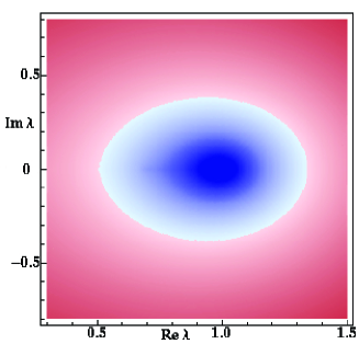
Figure 5: The mixed transverse exponent $\chi$ as a function of $\lambda$ for the dynamics (21) and the parameter values $\alpha=100$, $\beta=20$, $\epsilon=-1$. Blue indicates negatives values of $\chi$ and red positives values, respectively.

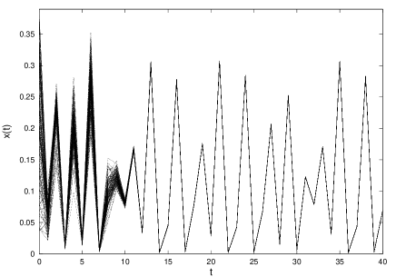
Figure 6: Dynamics of a random directed network of 100 sigmoidal neurons with both positive and negative weights, showing synchronization to a chaotic trajectory starting from random initial conditions. Parameter values are as in fig. 5.

VII Suppression of chaos via synchronization

Besides the emergence of chaos in networks of simple units, our theory can also be used to show the possibility of simple synchronous dynamics in a network of chaotic units. In other words, chaos is replaced by simpler behavior in the network. The field of chaos control is extensive and includes several well-established methods; for an overview see Schoell07 and the references therein. In our case, the network achieves chaos suppression through synchronization of its units.

As an example we study chaos suppression in a network of coupled chaotic logistic maps. It is well-known that the logistic map

$$\ell_{\rho}(x)=\rho x(1-x),\;\;\rho\in[0,4]\mbox{ and }x\in[0,1],$$ (22)

undergoes a period doubling route to chaos as the parameter $\rho$ is increased from 0 to 4 Devaney89 . In the sequel we will consider two different values for the parameter $\rho$. For $\rho=2.5$ the logistic map possesses an attracting fixed point and the Lyapunov exponent is given by $\mu_{\ell_{2.5}}=-\ln 2$. Thus $\ell_{2.5}(x)$ is dynamically simple. On the other hand for $\rho=4$ the logistic map is maximally chaotic with a Lyapunov exponent $\mu_{\ell_{4}}=\ln 2$.

Consider a network of chaotic logistic maps, with $f(x)=g(x)=4x(1-x)$ and $\epsilon=-3/8$. In this case the synchronous solution is given by $s(t)=\ell_{2.5}(t)$. So the whole synchronized network displays simple dynamical behavior, although all units in the network are chaotic. It follows from (13) and (14) that the network synchronizes if all eigenvalues $\lambda_{k}$, for $k\geq 2$, are contained in $\mathcal{D}(-5/3,10/3)$.

VIII Synchronization condition without eigenvalue calculations

As we have seen, the synchronous solution can be simple although all units of the network are chaotic. In this case it is possible to state a sufficient condition for synchronization without the explicit calculation of the Laplacian eigenvalues. It follows from Gershgorin’s disk theorem Horn90 that all eigenvalues of $\mathcal{L}$ are contained in $\mathcal{D}(1,r)$, where

$$r:=\max_{i}\frac{\sum_{j}|w_{ij}|}{|\sum_{j}w_{ij}|}.$$ (23)

On the other hand, by (13) and (14), the system synchronizes if all eigenvalues $\lambda_{k}$, for $k\geq 2$, of $\mathcal{L}$ are contained in $\mathcal{D}(c^{*},r^{*})$. Consequently, a sufficient condition for synchronization is given by

$$\mathcal{D}(1,r)\subset\mathcal{D}(c^{*},r^{*}).$$ (24)

We consider the case where $g(x)=cf(x)$. In Bauer08b we prove that (24) holds if and only if

$$\mu_{(1+\epsilon c)f}<\log\left|\frac{1+\epsilon c}{1+|\epsilon c|r}\right|.$$ (25)

Note that (25) can only be satisfied if the resulting synchronous behavior is not chaotic, since the right-hand-side of (25) is non-positive. Hence, if the synchronized solution $s(t)$ is not chaotic, it is possible to use the spectral bound $r$, instead of the whole spectrum of $\mathcal{L}$, to give a sufficient condition for synchronization. The advantage is that from (23) one can immediately estimate the effect of changing the network weights without lengthy eigenvalue calculations.

IX Discussion

In diffusively-coupled networks, the whole synchronized network displays the same behavior as any single individual unit; hence, complex behavior cannot emerge through synchronization of dynamically simple units. In contrast, as we have shown in this letter, the direct-coupling scheme leads to new collective dynamical behavior when the network synchronizes. We have given an analytical condition for synchronization in terms of the spectrum of the generalized graph Laplacian and the dynamical properties of the individual units and coupling functions. In particular, we have shown that synchronous chaotic behavior can emerge in networks of simple units, and conversely, chaos can be suppressed in networks of chaotic units through synchronization. These results represent a further step towards answering a fundamental question in complexity, namely, how complex collective behavior emerges in networks of simple units.

The setting presented here allows for studying synchronization in general network architectures. Such generality is important for applications because the connection structure of many real-world networks is unidirectional and the influence of neighboring units can be excitatory or inhibitory, as in neuronal networks. We have applied our theoretical findings to two neuronal network models, and have shown that, by changing a single parameter such as the coupling constant, the network can exhibit quite a rich range of dynamical behavior in its synchronized state. The results presented here provide insight on how new dynamical behavior may be induced in neuronal networks by changing the synaptic coupling strengths in a learning process.

References

- (1) A. Arenas, A. Diaz-Guilera, J. Kurths, Y. Moreno, and C. Zhou. Synchronization in complex networks. Physics Reports, 469:93–153, 2008.
- (2) D. G. Aronson, G. B. Ermentrout, and N. Kopell. Amplitude response of coupled oscillators. Physica D, 41:403–449, 1990.
- (3) F. M. Atay, J. Jost, and A. Wende. Delays, connection topology, and synchronization of coupled chaotic maps. Physical Review Letters, 92:144101, 2004.
- (4) F. M. Atay and Ö. Karabacak. Stability of coupled map networks with delays. SIAM J. Applied Dynamical Systems, 5(3):508–527, 2006.
- (5) F. Bauer. Spectral properties of the normalized graph laplace operator of directed graphs. In preparation.
- (6) F. Bauer, F. M. Atay, and J. Jost. Synchronization in time-discrete networks with general pairwise coupling. Nonlinearity, 22:2333–2351, 2009.
- (7) S. Boccaletti, J. Kurths, G. Osipov, D. L. Valladares, and C. S. Zhou. The synchronization of chaotic systems. Physics Reports, 366(1-2):1 – 101, 2002.
- (8) M. Chavez, D. Hwang, and S. Boccaletti. Synchronization processes in complex systems. Eur. Phys. J. Special Topics, 146:129–144, 2007.
- (9) Fan R. K. Chung. Spectral Graph Theory (CBMS Regional Conference Series in Mathematics, No. 92). American Mathematical Society, 1997.
- (10) Peter Dayan and L.F. Abbott. Theoretical neuroscience: Computational and mathematical modeling of neural systems. MIT Press, Cambridge, 2001.
- (11) R. Devaney. An introduction to chaotic dynamical systems - second edition. Addison Wesley, 1989.
- (12) Roger A. Horn and Charles R. Johnson. Matrix analysis. Cambridge University Press, Cambridge, 1990.
- (13) K. Kaneko. Clustering, coding, switching, hierarchical ordering, and control in a network of chaotic elements. Physica D, 41:137–172, 1990.
- (14) X. Li, G. Chen, and K. Ko. Transition to chaos in complex dynamical networks. Physica A, 338:367–378, 2004.
- (15) W. Lu, F. M. Atay, and J. Jost. Synchronization of discrete-time dynamical networks with time-varying couplings. SIAM J. Math. Anal., 39(4):1231–1259, 2007.
- (16) F. Pasemann. A simple chaotic neuron. Physica D, 104:205–211, 1997.
- (17) L. Pecora and T. Carroll. Synchronization in chaotic systems. Phys. Rev. Lett., 64:821–824, 1990.
- (18) Louis M. Pecora and Thomas L. Carroll. Master stability functions for synchronized coupled systems. Phys. Rev. Lett., 80(10):2109–2112, 1998.
- (19) Arkady Pikovsky, Michael Rosenblum, and Jürgen Kurths. Synchronization : A Universal Concept in Nonlinear Sciences (Cambridge Nonlinear Science Series). Cambridge University Press, 2003.
- (20) E. Schöll and H.G. Schuster. Handbook of chaos control, 2nd edition. Wiley-Vch, 2007.
- (21) J. Sun, E.M. Bollt, and T. Nishikawa. Master stability functions for coupled nearly identical dynamical systems. EPL, 85(60011), 2009.
- (22) X. Wang. Period-doublings to chaos in a simple neural network: an analytical proof. Complex Systems, 5:425–441, 1991.