The complex behaviour of the microquasar GRS 1915+105 in the $\rho$ class observed with BeppoSAX. I: Timing analysis

GRS 1915+105 was observed by BeppoSAX  for about 10 days in October 2000. For about 80% of the time, the source was in the variability class $\rho$, characterised by a series of recurrent bursts. We describe the results of the timing analysis performed on the MECS (1.6–10 keV) and PDS (15–100 keV) data. The X-ray count rate from GRS 1915+105 showed an increasing trend with different characteristics in the various energy bands: in the bands (1.6–3 keV) and (15–100 keV), it was nearly stable in the first part of the pointing and increased in a rather short time by about 20%, while in the energy range (3–10 keV) the increase had a smoother trend.
Fourier and wavelet analyses detect a variation in the recurrence time of the bursts, from 45–50 s to about 75 s, which appear well correlated with the count rate. From the power distribution of peaks in Fourier periodograms and wavelet spectra, we distinguished between the regular and irregular variability modes of the $\rho$ class, which are related to variations in the count rate in the 3–10 keV range.
We identified two components in the burst structure: the slow leading trail, and the pulse, superimposed on a rather stable level. Pulses are generally structured in a series of peaks and their number is related to the regularity modes: the mean number of peaks is lower than 2 in the regular mode and increases up to values higher than 3 in the irregular mode. We found that the change in the recurrence time of the regular mode is caused by the slow leading trails, while the duration of the pulse phase remains far more stable. The evolution in the mean count rates shows that the time behaviour of both the leading trail and the baseline level are very similar to those observed in the 1.6–3 and 15–100 keV ranges, while that of the pulse follows the peak number.
These differences in the time behaviour and count rates at different energies indicate that the process responsible for the pulses must produce the strongest emission between 3 and 10 keV, while that associated with both the leading trail and the baseline dominates at lower and higher energies.

1 Introduction

The galactic microquasar GRS 1915+105 was discovered in 1992 in the hard X-ray band (Castro-Tirado, Brandt & Lund 1992). VLA images of the radio counterpart showed two opposite radio jets moving at an apparent superluminal velocity, and from their proper motions both a distance of about 12 kpc and an inclination angle to the line of sight of about 70^∘ were inferred (Mirabel & Rodriguez 1994).

The optical counterpart was identified by Castro-Tirado et al. (2001) with a binary system of orbital period about 33 days (Greiner, Cuby & McCaughrean 2001) containing a black hole whose estimated mass is 14.0$\pm$4.4 $M_{\odot}$ (Harlaftis & Greiner 2004). The X-ray behaviour of GRS 1915+105 is characterised by strong variability with very bright and quiet phases. The spectrum is generally fitted by at least two components: a multi-temperature disk black body and a power law (possibly with a variable exponential cut-off) extending up to several hundreds keV. During the bursts, the main spectral parameters of the thermal component exhibit significant variations, which were interpreted as representing the emptying and refilling of the inner portion of the accretion disk (Belloni et al. 1997a). Quasi-periodic oscillations were observed with the PCA experiment onboard RXTE at frequencies up to above 100 Hz (Morgan, Remillard & Greiner 1997; McClintock & Remillard 2006) and a strong signal around 67 Hz, also studied by Belloni, Mńdez & Sánchez-Fernadez (2001). A detailed account of the main properties and modelling of GRS 1915+105 can be found in the review paper by Fender & Belloni (2004).

Using a large collection of RXTE observations, Belloni et al. (2000) defined 12 different variability classes of X-ray emission, each of them characterised by a time profile and spectral variability inferred from the dynamical hardness ratio plots. This classification is potentially useful for describing the behaviour of this exceptional source and for understanding the physical processes responsible for the X-ray emission, so we will refer to it when presenting our results. These 12 variability classes, however, do not exhaust the very rich set of temporal patterns exhibited by GRS 1915+105: Klein-Wolt et al. (2002) and Hannikainen et al. (2003, 2005) reported two other variability classes. Furthermore, GRS 1915+105 exhibits a wide variety of complex behaviours when class transitions occur.

GRS 1915+105 was observed by the Narrow Field Instruments (NFIs) onboard the BeppoSAX  satellite (Boella et al. 1997a) on several occasions (Feroci et al. 1999, 2001; Ueda et al. 2002). The amount of data collected during these pointings is very large and requires a long and complex analysis. In the present article, we report the results of an analysis of the time behaviour of GRS 1915+105 observed in the course of a long pointing in October 2000. On that occasion the source was mainly observed in the $\rho$ class (Belloni et al. 2000), which is characterised by a series of bursts, with a variable recurrence time from 40 to more than 100 seconds. The time profile of the bursts has a rather smooth rising branch (also named a ‘shoulder’) followed by a series of intense and short peaks with a fast decline.

The first observation of GRS 1915+105 in the $\rho$ class reported in the literature was performed on 15 0ctober 1996 with Rossi-XTE (Taam, Chen & Swank 1997) and the bursts exhibit a typical structure with two and more peaks. Their typical profile in the 2–13 keV band also differed from that in the 13-60 keV band. Belloni et al. (1997a,b) and Taam, Chen & Swank (1997) interpreted this bursting activity as the result of thermal/viscous instabilities in an accretion disk, in general agreement with the expectations of previous theoretical calculations (Taam & Lin 1984).

Other RXTE observations of the same class were described by Vilhu & Nevalainen (1998), Paul et al. (1998), and Yadav et al. (1999), who presented the results of a long pointing of GRS 1915+105 performed in June 1997 with the IXAE onboard the IRS-P3 satellite. On that occasion the source was in the $\rho$ class for about five days, then changed to the $\kappa$ class in which it remained for a similar time and afterwards returned to the former one. Transitions from/to the $\rho$ class to/from other classes were described by Naik et al. (2002), Chakrabarti et al. (2004, 2005), and Rodriguez et al. (2008).

A complete analysis of the timing and spectral properties of the $\rho$ class has yet to be performed. The long and nearly continuous data set, not yet published, presented and analysed in this paper is unique for investigating the behaviour of GRS 1915+105 in this particular variability class. Because of the richness of the data set, we applied several techniques to obtain an as complete as possible picture of the burst phenomenon, practically impossible to describe in a single paper. In this work, we studied the timing properties covering a range of timescales from a few seconds to a few days. We first investigated the variations in the mean brightness in different spectral bands on the timescale of a day and we then applied Fourier periodograms and wavelet transforms to study the temporal properties of the X-ray light curves. Finally, we investigated the profile of the bursts, over a timescale of a few seconds, using a statistical approach. We searched for correlations between the timing behaviour of GRS 1915+105 and the X-ray brightness of the bursts, finding highly significant relations. All of these results are particularly useful for addressing either the spectral analysis or studying the onset of unstable phases in terms of chaotic processes. These subjects will be described in detail in a couple of forthcoming papers.

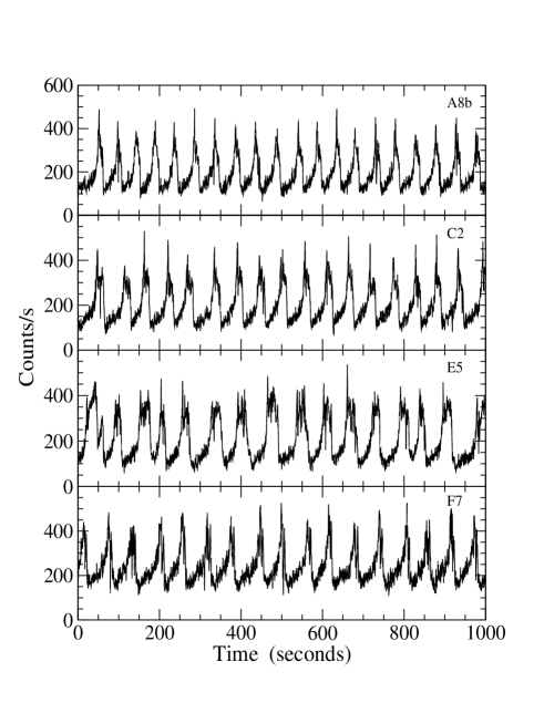
Figure 1: Segments of MECS (1.6–10 keV) light curves extracted from four data series (top to bottom: A8b, C2, E5 and F7) at different times during the BeppoSAX  observations of October 2000. Time bin width is 0.5 s and the starting time of each segment is arbitrarily selected within the series. Note that the first two and the fourth panels exhibit the characteristic time profile of the $\rho$ class, while the third panel has a more complex structure.

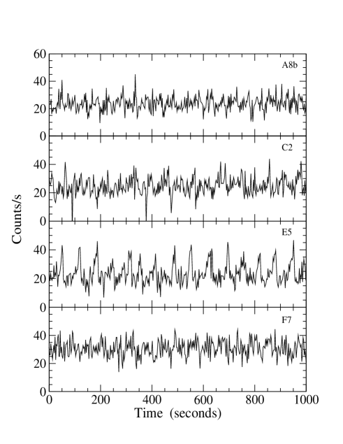
Figure 2: Segments of PDS (15–100 keV) light curves extracted from the same times series of Fig. 1. Time bin width is 2.5 s. Note that individual bursts are more apparent in the E5 series (thid panel) than in the other three.

2 The observations

The BeppoSAX  observation of GRS 1915+105 considered in the present paper started on October 20, 2000 (MJD 51837.894) and terminated on October 29 after an overall duration of 768.79 ks. The observation consisted of several runs of a typical duration of about one day. Each run is identified by a numeric code and consists of data segments corresponding to the visibility intervals of the source along the satellite orbit. The data obtained with all the NFIs can be retrived from the BeppoSAX  archive at the ASI Science Data Center.

In this paper, we limit our analysis to the data obtained in the first six runs and partially in the seventh one for a total duration of about 610,000 seconds, which covers about the 80% of the entire pointing. The net MECS exposure time is 257 ks, while the PDS net exposure amounts to 123 ks. This choice is motivated by, in this period, GRS 1915+105 remaining mainly in the $\rho$ class with some phases of instability similar to the $\kappa$ class. In the data acquared during the last few orbits of the seventh run and during the two remaining ones, the source changed to other and more complex classes and therefore, will be analysed in a forthcoming paper. The log of the observation runs considered in the present paper (see Table A.1) as well as the details of the data reduction are reported in Appendix I.

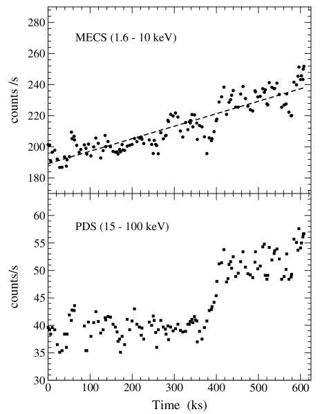
Figure 3: Long-term evolution of the X-ray count rates of GRS 1915+105 during the long observation of October 2000 in the MECS (upper panel) and PDS (lower panel) energy bands. The dashed line indicates the linear best-fit to MECS data. In the PDS data, two brightness states are evident with a short transition between them, occurring between 375 and about 400 ks.

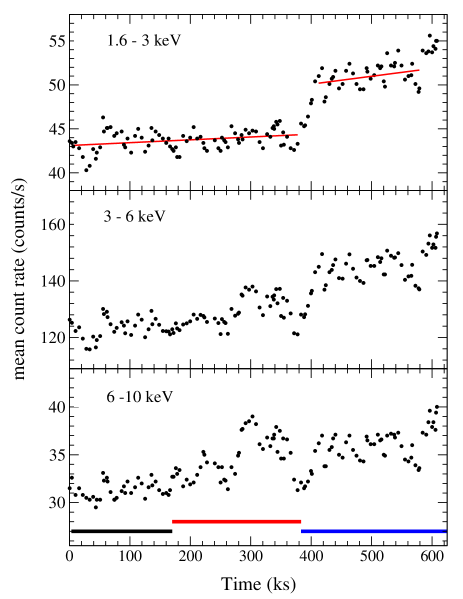
Figure 4: The time evolution of the MECS mean count rate in three energy bands: 1.6–3 keV, 3–6 keV and 6–10 keV (top to bottom). The two lines (red in the electronic version) in the upper panel are the linear best fits in the corresponding intervals. The thick horizontal lines (black, red and blue in the e-version) in the bottom panel indicate the three time segments used in our analysis of the data: the second interval includes the local excess of count rate.

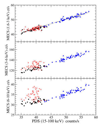
Figure 5: The mean MECS count rates in the three bands 1.6-3 keV (top panel), 3-6 keV (middle panel), and 6-10 keV (bottom panel) plotted against that of PDS. The three symbols and colours corresponds to the data of the three time intervals of the MECS: first interval (black filled squares), second interval (red open circles), third interval (blue filled triangles).

It is practically impossible to describe completely this enormous amount of data and therefore we developed a rather simple classification scheme for the timing properties of individual segments based on Fourier and wavelet analyses. To achieve a clearer understanding, however, we selected some data series that are representative of the different behaviour of GRS 1915+105 and used them as examples throughout this paper. These series are named A8b, C2, E5, and F7 (see Appendix II and Table A.2) and some portions of them are of equal length, 1,000 seconds, as shown in Fig. 1, for the MECS and in Fig. 2 for the PDS, for which a time binning greater than MECS was used to increase the signal to noise ratio (S/N). It is possible that the source exhibited the behaviour characteristic of the $\rho$ class of Belloni et al. (2000). We note, however that the light curve in the third panel (E5) exhibits behaviour intermediate between this and the $\kappa$ class, characterised by broad and slow bursts. The S/N of PDS data is poorer than MECS and the bursts of A8b, C2, and F7 segments are barely apparent, while those of the E5 segment are all clearly distinguishable. As discussed later, this finding is a consequence of a spectral evolution related to the behaviour of the source; we also note that bursts in PDS series appear sharper than those of the MECS.

In the various panels in Figs. 1 and 2, there is an important indication of the change in the mean flux of the source. Both of the last data series (F7) have count rates that are significantly higher than the other three. In particular, the series in Fig. 1 shows an increase in the minimum level of about 30% from $\sim$120 counts/s in the series A8b to $\sim$165 counts/s in F7, while the bursts’ height does not show a comparable increase.

3 Slow variations

The X-ray flux from GRS 1915+105 varied during the observation, exhibiting a generally increasing trend with superimposed variations on timescales of a few hours. Changes occurring on the scale of one day or longer (slow variations) are evident from the evolution in the count rate in the MECS and PDS bands averaged over each time segment. Figure 3 shows the count rate history of the MECS (1.6–10 keV) and PDS (15 – 100 keV) energy bands. The mean count rate of the MECS, computed only from time series longer than 500 seconds, increased from $\sim$200 counts/s at the beginning of the observation to reach $\sim$250 counts/s at the end. It can be described by a linear interpolation (the linear correlation coefficient is $r$=0.884) with a positive rate of $\sim$7 (counts/s)/day.

The evolution in the mean PDS count rate appears to be different from that of the MECS and shows two rather long states of different intensity: in the first one, the mean count rate varied between 35 and 44 counts/s, whereas in the second state it was between 48 and 57 counts/s. These two states are separated by a relatively fast transition that started at about 375 ks after the beginning of the pointing and lasted about 30 ks, thus including the time series from E7 to E12. The mean PDS count rate changed from the average value 39.4 and a standard deviation of 1.9, to 51.7 and 2.7, respectively, with a corresponding luminosity increase above 15 keV by about 30%.

To obtain a clearer description of these different behaviours, it is useful to consider the count rate evolution in three narrow bands of the MECS, of nominal energies of 1.6–3, 3–6, and 6–10 keV (the correspondence with the true photon energy being good because the instrumental response matrix is essentially diagonal) and selected to have a sufficiently high S/N. The resulting plots are shown in the three panels of Fig. 4 and some interesting differences appear between them. The low energy plot is remarkably similar to that of the PDS: the mean count rate was almost constant around 43 counts/s up to $\sim$375 ks, then increased over about 30 ks to $\sim$51 counts/s and fluctuated around this high level until the end. In the intermediate and high energy ranges, the count rate evolution is much closer to the general MECS trend. At energies higher than 6 keV, however, the count rate in the central part of the observation had a mean level of around 38 counts/s, higher than in the previous portion ($\sim$32 counts/s). This high level finished just before the fast increase in the low energy and PDS curves. A similar change can also be recognized in the intermediate band, but is absent both at lower energies and in the PDS. To take this feature into account, we divided the entire observation into three intervals: the first interval extends from the beginning to about 170 ks and includes the series up to B15a, the second from $\sim$170 ks to $\sim$380 ks, includes the entire bump in the 6-10 keV band (series B15b to E7), the third interval covers the remaining time from the series E8 until the end. These intervals are indicated by the three horizontal lines in the bottom panel of Fig. 4.

The differences between the various energy bands become clearer in plots that compare the mean count rates in three MECS bands with in the PDS band (Fig. 5). As expected from the similar time evolution, the 1.6–3 keV MECS and PDS count rates have a strong positive correlation: the linear correlation coefficient is $r=0.974$, confirming the very tight relationship. Similar trends are also exhibited by the count rates in the two other MECS bands with the exception of the data points in the second interval, which do not follow the correlation and show an increase in scatter with energy. There are, however, some points in the second interval with a rather low count rate that are mixed with those of the first interval. These series occurred in the first part of the interval and their behaviour was remarkably similar to that which is typical of series in the first interval. These results can be assumed to be indicative of a close relation between the processes responsible for the emission below $\sim$3 keV and above 15 keV, while in the range (3–15 keV) an additional contribution of a different origin can occasionally be observed.

4 Fourier and wavelet classification

The first approach to investigating the timescales of the burst sequence in each data series is to derive the Fourier power spectra or periodograms. The different appearance of these periodograms lead us to introduce a practical classification of series that is useful to a synthetic description of the variability in GRS 1915+105 in the course of the observation. This classification is also useful to the study of the chaotic states that appear in the complex limit-cycle phenomenology. We argue that the GRS 1915+105 system in the $\rho$ state can also exhibit states with chaotic properties (see, the analysis of Misra et al. 2006), as we will discuss in future work.

In several data series, however, there are large variations from one burst to the subsequent one that are not described well by the corresponding periodogram. To obtain more information about variations occurring on scales of between a few tens and hundreds of seconds, we applied the wavelet transform and devised a more complete two parameter classification.

4.1 Fourier periodograms and classification

A large fraction of the Fourier periodograms (hereafter FP) exhibit a single dominant peak, indicating that bursts occurred with a rather stable recurrence time, $T_{rec}$. In contrast other spectra have two or more dominant features that do not correspond to the harmonics of the main peak. We prefer to use the term recurrence time instead of ‘period’ because the burst sequence has never been observed to remain very stable for time intervals of about one hour, as shown by the wavelet analysis presented in Sect. 4.2. In Table A.3, we reported the values of $T_{rec}$and the corresponding FP time resolution $\Delta t$ that is an estimate of the uncertainty. As illustrated by the classification scheme presented in Appendix III, we introduced three types of periodograms according to the power distribution: S type when only one dominant peak is apparent in the FP, T type when two peaks are present, and M type for a higher peak number. Figure 6 shows the FPs of the four MECS data series plotted in Fig. 1: the first FP is of S type, the third of M type, and the remainder are both of T type with different peak heights and separation.

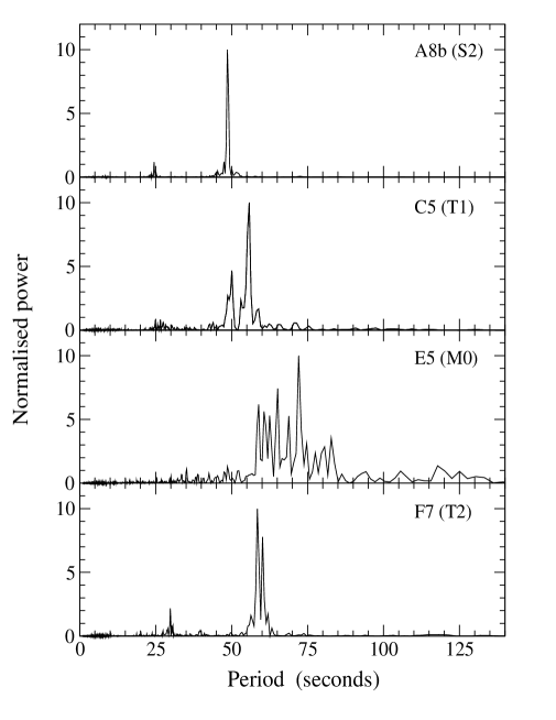
Figure 6: Periodograms of four MECS time segments shown in Fig. 1. The spectral classification based on Fourier periodograms and wavelet scalograms in reported in parenthesis.

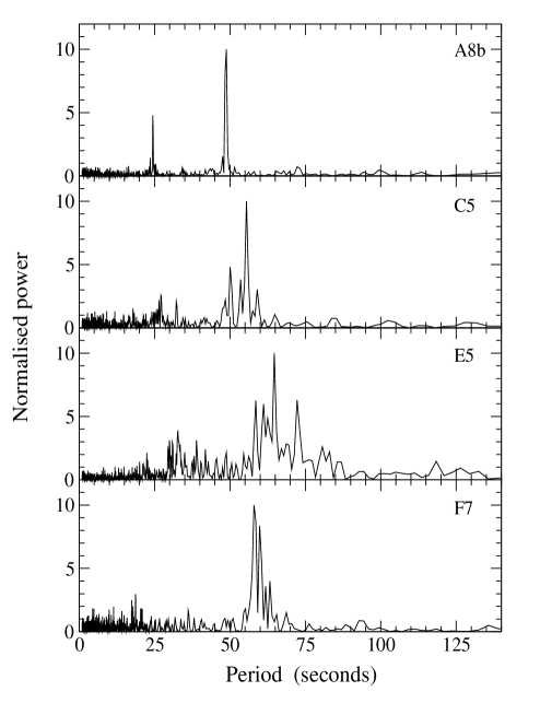
Figure 7: Periodograms of four PDS time segments (from top to bottom) A8b, C2, E5, F7. Note the similarity of power distributions with those of Fig. 3 despite the lower S/N.

We computed the FPs for the PDS time series with durations comparable to those of the corresponding MECS series. Their classification, however, is not as good as for the MECS because of the low S/N ratio. Figure 7 shows the FPs of the already considered four series: significant peaks are present at the same periods as those of the MECS series, although the power distributions between the peaks differ. We note that the power at the first harmonic in the PDS periodograms is generally higher than in the MECS.

An interesting result is the change of $T_{rec}$  in the course of the pointing. In Fig. 8, the values of $T_{rec}$  are plotted as a function of time for the three intervals using different symbol in order to distinguish the type of each series. In the first interval, $T_{rec}$  is rather stable, while in the second the dispersion of $T_{rec}$  and the width of the peak ranges of M series are much higher than in the other two. We note that, as in Fig. 5, some series in the initial portion of this latter interval, have $T_{rec}$  values close to those found in the first interval. In the third interval, the recurrence time exhibits a generally increasing trend.

As shown in Sect. 3, the mean count rate increases during the pointing and one can therefore expect that it should be correlated with $T_{rec}$. In Fig. 9, $T_{rec}$  is plotted against the MECS (for the two bands 1.6–3 and 3–10 keV) and PDS count rates. In the second interval, no correlation is apparent, while it is clearly apparent in the third interval. The linear correlation coefficient is around $r=0.89$ for all three energy bands. We note also the similarity between the first and the third panel of Fig. 9, which confirms the strong relation between the lowest MECS and PDS energy ranges.

The FP classification does not provide a univocal description of the source behaviour: in a few cases, we found series with an apparently irregular sequence of bursts (e.g., D3a or D8b) but the power mostly concentrated in a single peak. It was therefore necessary to improve the classification by taking account of how the power is distributed over the various timescales in the course of the series, whereas the standard Fourier analysis considers the entire series. This analysis can be performed by means of wavelet transforms and the results are described in the following.

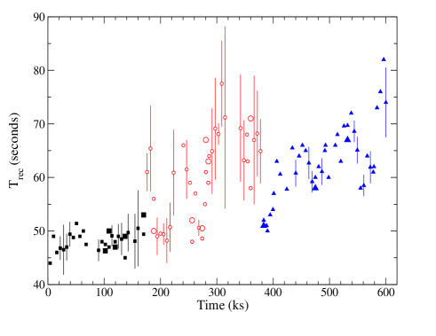
Figure 8: The evolution in the recurrence time of the MECS series in the course of the observation. Along the abscissa, we plot is the time elapsed since the beginning of the observation. Symbols indicate series of three time intervals: first interval (filled black squares) including series from A1b to C6, second interval (open red circles) including series from C7 to E7, and a third interval (filled blue triangles) including series to G12c. For the T series, the recurrence times of both peaks are plotted (using symbols of different size), whereas the points of M series correspond to the centroid value as given in Table A.3 and the vertical bar to the amplitude of the range.

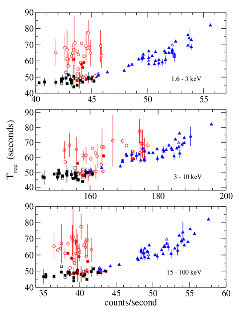
Figure 9: The relations between the recurrence time and the mean count rates in the energy bands. Top to bottom: MECS 1.6–3 keV, MECS 3–10 keV, PDS 15–100 keV. Data symbols correspond to the three time intervals defined in text (see also Fig. 4).

4.2 Wavelet spectra and their classification

The wavelet transform permits us to decompose a signal using a localized function. Standard wavelet analysis is based on the computation of wavelet power spectra (also named wavelet scalograms, hereafter WS) defined as the normalised square of the modulus of the wavelet transform. A short description of the algorithm and definitions of the spectral quantities are given in Appendix IV. An advantage of this local analysis is that scalograms are less sensitive to telemetry gaps than FP and it is possible to consider longer time series.

The WSs for three of the MECS time series in Fig. 1 (A8b, E5, F7) are presented in the left-hand side panels of Fig. 10: each spectrum consists of a two dimensional map where the curves of equal power define regions coded in color/grey scale. Because of the smoothing and interpolation necessary to draw these curves, these plots provide a qualitative description of the evolution of the power during the time series.

The differences between both the S and T series and the M series are clearly apparent: the two former types are characterised by an uninterrupted and nearly horizontal strip, centred on a timescale length close to the $T_{rec}$  estimated from periodograms. The coarser resolution of WSs compared to FPs does not allow us to identify clearly the peak separation in the T series, which is only 2 s (panel 3). However, a decrease in the highest power timescale is discernible around 1700 seconds. Another strip of lower intensity is centred around the half value of $T_{rec}$  and corresponds to the first harmonic. Small changes in $T_{rec}$  are also present in the WS of the S series, although their duration is limited to only a few bursts, too short to produce a separate peak in the FP. It is unclear whether there is a sort of slow modulation of the recurrence time of subsequent bursts. In some cases, these changes occur on timescales longer than the duration of two or three bursts.

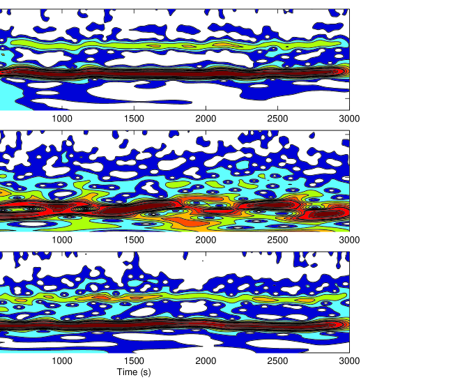
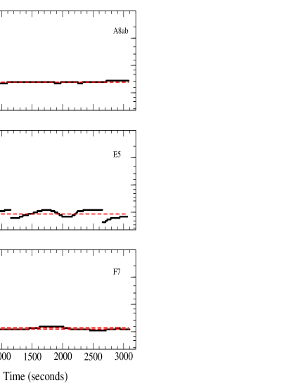
Figure 10: Left panel: iso-power representation of the scalograms of three MECS time series A8ab (the two series are joined together), E5 and F7 (top to bottom), plotted in Fig.1. In each spectrum, the time scale increases towards the bottom. The dark strip indicates the region where the highest power is found and corresponds to $T_{rec}$; the strip of the first harmonics is also clearly visible in the top and bottom panels, whereas it is not present in the highly irregular E5 series. Right panel: time evolution of the timescales of the power maxima in the scalograms of the three series in the left panel: $T_{j,max}$ increases with a log scale towards the bottom to permit a clearer comparison with the spectra in the left panel. Dashed lines represent the values of the $T_{rec}$  peaks or the peak centroid from Fourier periodograms.

The M series have typically a far more irregular pattern also over short time intervals. As for the E5 series in Fig. 10, power is concentrated within a rather broad strip that exhibits meanderings, bifurcations, and interruptions corresponding to short and long recurrence intervals between subsequent bursts. A fraction of the power that is greater than in the two other cases is present on both long and short timescales, and no strip corresponds to the first harmonics.

To evaluate the stability of the time series from WSs, we adopted a criterium based on the relative variance ratio $R_{w}$ (see Appendix IV). There is a correspondence between the values of $R_{w}$ and the periodogram classification: this parameter tends to increase between the series S and T, and between the series T and M. The presence of a single dominant peak is not necessarily indicative of a stable signal: a series can exhibit large instabilities occurring within a rather small time interval or frequent changes in $T_{rec}$  but with a rather stable mean value. On the other hand, more peaks in the FP occurring with a rather narrow range can correspond to small variations in the recurrence time without a large modification of the bursts’ structure. To take this variety of behaviour into account we defined three classes, indicated by 0, 1, and 2 in order of increasing stability (see Appendix IV). The majority of S spectra, 30 among 45, are of S2 type, 12 are S1, and 3 S0; we also note that 10 of the S1 spectra have $R_{w}$ smaller than 4.0, indicating that their $T_{rec}$  is only moderately unstable. In contrast, M series are of class 0 and 1, and only four are of class 2 but with $R_{w}$ values larger than 2.5. Nine spectra of T series are of class 1, confirming their intermediate type between S and M. The complete classification of the spectra in Fig. 10 is indicated by the labels of Fig. 6.

The results presented in this and previous Sections suggest that one can consider two modes of the $\rho$ class, which we call regular and irregular modes. The former is associated with the occurrence of S or T spectra of stability class 1 or 2, the latter with M series or stability class 0.

5 Analysis of the burst structure

It is also important to study how the burst structure changes in the various modes. As pointed out by Belloni et al. (2000), the individual bursts, when analysed with sufficient time resolution, exhibit several substructures, such as sharp spikes and dips, of durations as short as to a few hundreds of milliseconds, and probably even shorter. These substructures are highly variable and therefore it is practically impossible to study the structure of thousands of bursts with a high time resolution. We adopted the two following approaches: we first performed a statistical study of a large sample of bursts to describe their mean properties, and afterwards studied the structure of some typical bursts of two of the selected time series to take account of the energy dependence.

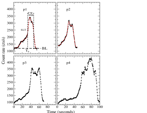
Figure 11: Four examples of burst shapes after smoothing with peak number classification from p1 to p4. Best fits using 2 Gaussian components for the peak and a fourth degree polynomial for the slow leading trail are shown for the two upper bursts (dashed/red line).

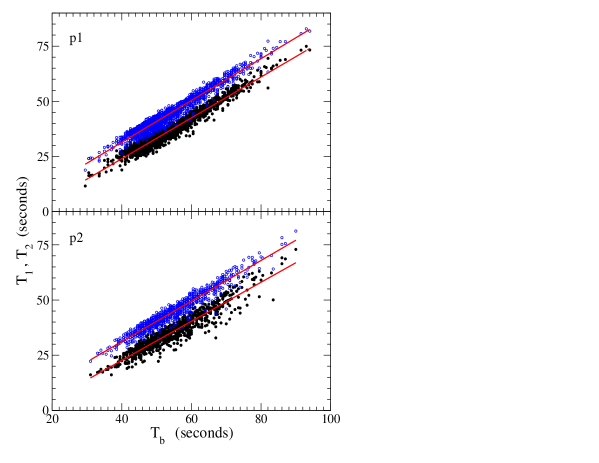
Figure 12: Plot of $T_{1}$ (black solid circles) and $T_{2}$ (open blue circles) versus $T_{b}$ showing the strong linear correlations of the central times of the two Gaussian curves with the total duration of the bursts. Times for p1 pulses are plotted in the upper panel and those for the p2 pulses in the lower panel. Linear best fits (in red) are also shown for each data set. The noticeable similarity of these data distributions indicates that there are no significant differences between these multiplicity classes.

5.1 The statistical analysis

To avoid the complications caused by the rich and variable substructures, a statistical analysis was performed after a running-average smoothing of all data series for the entire MECS energy band with a window of 5.5 seconds (11 time bins). Despite the complex structure, the burst shape after smoothing appears rather stable. We introduced peak number or “multiplicity” classes based on the number of distinguishable features in the smoothed profile. Examples of bursts of different multiplicity from 1 (hereafter indicated as p1) to 4 (p4) are shown in the various panels of Fig. 11. This classification was applied to all the 172 time series, for a total number of 4083 bursts, also because the series that are too short for the Fourier analysis still contain a large number of useful bursts.

We measured the duration $T_{b}$ of individual bursts starting from the initial minimum level, which is reached just after the decay tail of the preceding one. This minimum level was verified to be nicely constant in the course of each series. It defines a baseline level (BL) over which the bursts are superimposed. We also divided their typical structure into two parts: the shoulder or slow leading trail (SLT), which is followed by a Pulse (see examples of this partition in Fig. 11). For a small number of bursts, the identification of the end was tricky because there is a final and clearly separated pulse that occurs before the count rate has reached its lowest level. We called these bursts anomalous and excluded them from the shape analysis. A couple of anomalous bursts are clearly evident in the light curve of the E5 series shown in Fig. 1. Anomalous bursts are observed in the irregular mode and very rare or absent in the regular one.

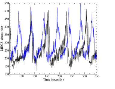
Figure 13: Comparison between two short segments of equal duration of the S2 series A8b (blue) and G9 (black) time series characterised by very different $T_{rec}$  and mean count rates. The A8b light curve has been shifted upward by 90 ct/s to match the peaks’ height. Note the very good agreement between the pulse shapes of the two series, in contrast to the leading edge being much longer in G9 than in A8b. The bin width is 0.5 s.

Pulses, examined at high time resolution, have typical structures consisting of a sequence of peaks of variable height and duration, but when studied over a timescale of a few seconds they have more stable profiles, such as those in Fig. 11. Pulses of p1 and p2 bursts were modelled by a combination of two Gaussian curves and a fourth degree polynomial was used to reproduce SLT, which terminated at the half maximum height of the pulse. Best-fit curves are shown in the upper panels of Fig. 11: the need of the two Gaussian components for both p1 and p2 bursts is evident. We did not calculate best fits for bursts of type p3 or higher because they required additional Gaussian components and in some cases we did not obtain stable solutions.

A first relevant result of this analysis is that the central times $T_{1}$ and $T_{2}$ ($T_{2}>T_{1}$) of the two Gaussian components, measured starting from the initial time of the burst, are strongly correlated with the duration of individual bursts, measured to be the time separation $T_{b}$ between the minima of two subsequent bursts. The average $T_{b}$ in regular time series is very close to $T_{rec}$. Figure 12 shows a scatter plot of $T_{1}$ and $T_{2}$ against $T_{b}$ for the two considered multiplicities: the points are very well aligned along straight lines and no significant difference is evident between the two multiplicity classes. Linear correlation coefficients are very high ranging from 0.944 to 0.973. Best-fit linear relations have very similar slopes (within $\sim$3%) and this means that the difference $T_{2}-T_{1}$, which can be considered to be an estimate of the pulse width, is practically independent of $T_{b}$.

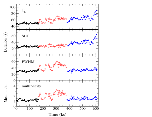
Figure 14: Time history of the durations of the various components of bursts (top to bottom): $\langle T_{b}\rangle$, mean SLT, mean pulses’ FWHM. The scales on the ordinates are identical to ease the comparison of data. In the fourth panel, we plot the evolution in the mean multiplicity of bursts. Symbols that identify the series in the three time intervals are the same as those of Fig. 5.

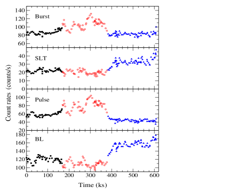
Figure 15: Time history of the mean MECS (1.6–10 keV) count rates of the various components after the subtraction of the BL (top to bottom): total burst, SLT, and the peak integral. The behaviour of the BL is shown in the last panel. The count rate scales in the three upper panels are equal, while that of the last one has been doubled in length. Symbol codes indicate the three time intervals as in the other figures.

This result implies that series of type S2, but with mainly different recurrence times, must have pulses of similar width. To illustrate this statement, we plot in Fig. 13 two short segments of the two S2 series A8b and G9: $T_{rec}$  is 49 s for the former and 73 s for the latter. Data were translated such that two bursts were superimposed two bursts: we note that they are of comparable height and width at variance with the SLT, which is much longer in the G9 series than in A8b.

The evolution of the durations and count rates of the various burst components, averaged over each data series, is presented in Figs. 14 and 15, respectively. We assumed that only data series with more than five bursts provide representative mean values. For bursts of multiplicity p3 or higher, for which no best-fit modelling was obtained, the durations of the FWHM were estimated directly from the smoothed profiles. The first panel in Fig. 14 shows the evolution of the mean $T_{b}$, which for the S and T series is similar to that of $T_{rec}$  (see Fig. 8), while the latter has a larger scatter for the M series. The duration of the SLT (second panel in Fig. 14) was far more regular: it increased very slowly from the beginning of the observation and this trend did not show appreciable changes in the second interval, while a moderate increase in the rate occurred in the third interval, which became higher one only in the last 40 ks. The mean FWMH of pulses (third panel), which was nearly constant in the first interval, showed large variations in the second interval: it increased for the first time after 170 ks from the beginning of the observation and returned to the previous values after a few series; it then increased again at about 250 ks and remained high for about 40 ks; a third high state was finally in the last and longest part of the second interval. In the third interval, the FWHM of the peaks returned to low values, but with a dispersion somewhat higher than in the first one, particularly approaching the end of the pointing. We also see in Figs. 14 and 15 that when the source was in the irregular mode the multiplicity of bursts increased and was strongly correlated with the pulse count rate. We recall that this particular behaviour represents the basis of the three interval segmentation introduced in Sect. 4.

We also analysed how the mean count rates in the entire MECS band of these components changed in the course of the pointing. To calculate the count rates of SLT and of pulses, it was first necessary to evaluate that of the BL, which for each piece of data was derived by averaging the count rates in the bins with the lowest level at the beginning of bursts.

The time history of the MECS BL count rate is shown in the bottom panel of Fig. 15: it is remarkably similar to that of the both PDS (Fig. 3) and the lowest energy range of the MECS (Fig. 4), despite the highest photon contribution is at energies between 3 and 10 keV. In particular, the mean BL did not show any increase in the second interval, when the behaviour of GRS 1915+105 was irregular. Thus, there is no indication of a positive correlation between the BL and the bursts’ multiplicity and duration. The evolution of the SLT and pulse count rates are given in the central panels of the same figure. In agreement with the previous results on the mean durations of these components, the SLT is highly correlated with the BL, while it is practically unaffected by the pulse amplitude and multiplicity. The mean pulse count rate has a very close correspondence with the multiplicity, and decreases from $\sim$55 to $\sim$45 counts/s from the first to the third interval, suggesting that it could be anticorrelated with the BL and SLT behaviour.

Our results do not disagree with those of Naik et al. (2002), who reported that the “burst strength” decreases for increasing $T_{rec}$. These authors define the “burst strength” as the ratio of the peak count rate to its lowest level. According to this definition, an increase in the BL and a rather stable pulse intensity would reduce the burst strength.

5.2 Energy dependence of the bursts’ structure

All the results derived in the previous analyses indicate that the burst structure must be energy dependent, and that the SLT and pulses should have different energy spectra. This property can be more accurately analysed by considering light curves at different energies. In Figs. 16 and 17, we plotted two short segments of series A8b and E5, respectively. The three panels in each figure correspond to the energy ranges considered above. Changes in the light curve structure are evident: at the lowest energies the count rate has a nearly triangular (or approximately sinusoidal) modulation clearly associated with the SLT and the bursts are located on the declining side. At higher energies, bursts become sharper and sharper, while the triangular modulation is reduced. In the irregular mode, the pulse sharpening is even more evident above 15 keV. Figure 18 compares two simultaneous segments of the MECS and PDS of the E5 series containing six bursts. As already found by Paul et al. (1998), bursts in both series occur at the same times, but those in the PDS are systematically narrower than those at lower energies. This effect cannot be entirely caused by the poorer S/N ratio of PDS data, as is clearly evident, for example, from the burst occurring at 180 s or that at 350 s. Moreover, PDS pulses appear generally at the end of the MECS bursts and this finding is in agreement with the spectral hardening in the course of the bursts. Paul et al. (1998) modelled the spectrum by a thermal emission from an accretion disk and described this phenomenon in terms of increasing temperature close to the end of the bursts.

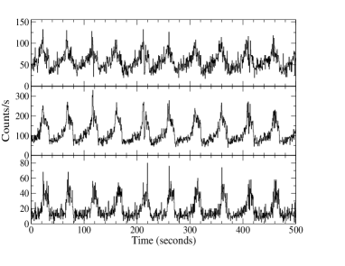
Figure 16: A short segment of the MECS A8b series in three energy bands: 1.6-3.0 keV (upper panel), 3.0-6.0 keV (central panel), and 6.0-10.0 keV (lower panel). The bin width 0.5 s for all sets. Note that in the highest energy range the SLT has practically disappeared and the pulses occur simultaneously with those at lower energies but their shape is sharper and duration is shorter.

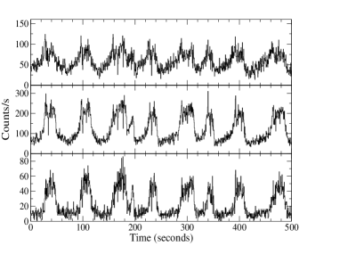
Figure 17: A short segment of the MECS E5 series in three energy bands: 1.6-3.0 keV (upper panel), 3.0-6.0 keV (central panel), and 6.0-10.0 keV (lower panel). The bin width 0.5 s for all sets. Note that in the highest energy range the SLT hss practically disappeared and the pulses occur simultaneously with those at lower energies but their shape is sharper and duration shorter.

To verify that bursts at higher energies are more sharply peaked than at lower energies, we computed the autocorrelation functions of the MECS and PDS E5 series because narrower bursts would correspond to shorter de-correlation times (zero crossing). These found to be equal to 16 s for the MECS and 10 s for the PDS. Similar differences were also observed for other irregular PDS series, in which individual bursts are clearly apparent.

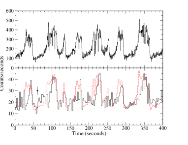
Figure 18: Comparison between MECS 1.6–10 keV (upper panel) and PDS 15–100 keV (lower panel) burst shapes of the E5 series. The latter has a bin width 2.5 s that reduces the statistical noise. Dashed line in the lower panel is the same portion of the rebinned MECS light curve scaled to PDS amplitude. Note that bursts in the higher energy range occur simultaneously with those at lower energies but their duration is generally shorter.

6 Summary and discussion

In October 2000, BeppoSAX  observed GRS 1915+105 continuously for about 10 days. For a large fraction of this time, the source exhibited the characteristic behaviour of the $\rho$ class defined in Belloni et al. (2000). In our analysis, the data obtained with the MECS and PDS were organised into a database including many series of duration corresponding to the spacecraft orbital windowing (or sometimes shorter because of telemetry gaps). We analysed these time series using Fourier periodograms and wavelet scalograms and introduced some simple criteria, based on the number and height of prominent peaks in the FPs and the variance ratio $R_{w}$ of scalograms, to classify the behaviour of GRS 1915+105. A complementary approach was the study of the characteristics of individual bursts, based on the definition of the two main components, namely the SLT (slow leading trail) and the pulse superimposed on a stable BL. Moreover, it was found to be useful to introduce an additional multiplicity classification based on the number of distinct features in the pulse.

We observed two different modes of the $\rho$ class: the regular and irregular mode defined according to the following characteristics. The regular mode scontains bursts with a nearly stable recurrence time $T_{rec}$  and the pulses have a multiplicity of 1 or 2, and only occasionally higher. Pulses are clearly detected in the energy range between 3 and 10 keV and are weak at lower as well as at higher energies. Below $\sim$3 keV, the shape of the signal modulation appears to be roughly triangular, pulses are small and occur around the maxima. In the irregular mode, the burst sequence does not have a stable recurrence time, the pulses have multiplicities generally greater than 2, and anomalous bursts appear. Pulses have harder spectra than in the regular mode, showing detectable emission above 15 keV in the PDS data, but have typically shorter durations than below 10 keV. The irregular mode in several ways resembles the $\kappa$ class (Belloni et al. 2000): it appears to be a transition state between the regular $\rho$ and the $\kappa$ class.

A classification of the burst types was introduced by Yadav et al. (1999), who considered only some observations of GRS 1915+105 that were typically shorter than one day. This work preceded the definition of variability classes by Belloni et al. (2000), and the light curves analysed by Yadav et al. (1999) belong to different classes.

Differently from our work, they classified as irregular the bursts of the $\kappa$ class, while as regular ones those of the $\mu$ and $\rho$ classes. They also found a correlation between the preceding quiescent time and the burst duration for their irregular type, whereas no such correlation was found for their regular ones. In our analysis, we considered only the $\rho$ class, and this led us to the discovery of some relevant relations between the typical timescales and the count rates in different energy bands.

The irregular mode was observed three times in our data (see Figs. 8, 14, and 15); during the rest of the observation, the source maintained itself in a regular mode. The first and shortest irregular phase started about 170 ks after the beginning of the observation and lasted only $\sim$15 ks; the second and third occurred between 220 and 260 ks and between 270 and 370 ks, respectively. Interestingly, the last transition from irregular to regular mode occurred in correspondence with a luminosity increase observed in the MECS (1.6–3 keV) and PDS light curves (see Fig. 4).

The behaviour of the source throughout our observation exhibits correlated signatures in both timing and intensity (i.e., count rates) domains. As an example, the recurrence time of bursts during the regular phase was found to have a positive correlation with the average MECS count rate (Fig. 9). On the other hand, the source intensity in different energy ranges exhibits a different behaviour: the rate below 3 keV correlates well with that above 15 keV (Figs. 3 and 4), and both of them exhibits a transition at the time $\sim$370 ks that also marks the last passage from the irregular to the regular modes. The intermediate energy range, 3–10 keV, appears to be unaffected by this transition in the timing parameters.

We found that the BL and SLT exhibit remarkably similar behaviours and the count rates are below 3 keV and above 15 keV. Instead, these two components appear to be unaffected by the pulse multiplicity, which is shown in our analysis to be capable of determining the duration of the pulse component. A signature of the time interval during which the multiplicity is highest (red open circles in the Figs. 14 and 15) is also clearly detected in the count rates of the pulse component of the bursts (the higher the multiplicity the higher the pulse count rate).

In the regular mode, we note that the increase in $T_{rec}$  is a consequence of the SLT duration (see Figs. 13 and 14), while the duration of the pulse component remains nearly stable. This implies that the characteristic timescales of these two components follow different variability patterns.

This intermingled set of correlations can be interpreted by introducing a two emission component scenario. A ‘stable component’ (shortly SC) is responsible for the triangular/sinusoidal modulated emission observed below 3 keV, and for the underlying BL emission (a clear separation between them is not possible from the present analysis). The other component, named the ‘pulsating component’ (or PC) appears with the pulses, which in the irregular mode they appear longer because of the higher number of peaks. In addition, the peaks that appear last in a pulse have harder spectra, because they are more evident above 15 keV than in the regular mode. It would be interesting to verify whether the onset of the PC is or is not related to the level reached by the SC, but our analysis was inconclusive on this subject.

The count rate plots in the various bands indicate that the energy spectra of SC and PC are expected to differ (see Figs. 16 and 17). In the 3–10 keV range, Taam, Chen & Swank (1997) already noticed a significant difference between the spectra of SLT and those of the pulses, the latter being harder, although in their analysis they did not consider the contribution of the BL. This result agrees with the changes in the hardness ratio in the course of the bursts, as reported by other authors (see, for instance, Paul et al. 1998). The average photon energy of the PC must be higher in the irregular mode than in the regular mode because pulses are more clearly detectable above 15 keV in that state. During the irregular mode, when the PC energy output was higher, the average count rate of the BL decreased suggesting that some mechanism of energy transfer from the SC to PC could be active in the source. All of these considerations are useful to the spectral analysis of the same data, which will be reported in a subsequent paper.

The results presented in this paper raise several interesting problems to explain the physical processes producing this complex behaviour of GRS 1915+105. From a theoretical point of view, following the first interpretation by Belloni et al. (1997a,b) and Taam, Chen & Swank (1997), the bursts of the $\rho$ class were modelled in terms of thermal-viscous instabilities in the accretion disk. Instabilities developing as series of pulses were investigated by several authors well before the discovery of GRS 1915+105. Taam & Lin (1984), Lasota & Pelat (1991) computed light curves very similar to those of GRS 1915+105 in the regular mode, identifying an SLT followed by a narrow peak. From the numerical calculations of Taam & Lin (1984), however, there is no clear indication that the recurrence time increases with the BL. These authors also found an increase in the pulse luminosity that is not observed in our results. About the two above components, SC would correspond to the BL joint with the pre-pulse emission, while PC is the overlying fast and prominent pulse. Watarai & Mineshige (2003) developed a model for GRS 1915+105, which includes an accretion disk around a 10 M_⊙ black hole, in which the viscosity stress has a functional relationship with the integrated pressure that is more general than in $\alpha$-disks. They considered a factor $(p_{gas}/p)^{\mu}$ ($0<\mu<1$) and calculated the light curves for some values of $\mu$: the recurrence time decreases by a factor of $\sim$2.5 for $\mu$ ranging from 0.1 to 0.2. However, according to their plot, the recurrence time decreases when both the DC level and pulse luminosity increase, which disagrees with our findings.

In the framework of the Belloni et al. (1997a,b) model, the burst sequence is interpreted as an emptying/refilling cycle of the inner portion of the accretion disk. In this context, the rise time - SLT in this work - is related to the viscous (disk-filling) timescale, which is proportional to the 3.5-power of the inner disk radius, while the pulse profile depends on the free-fall timescale, which scales linearly with the radius. From this point of view, the longer duration of SLT with respect to the pulse, is in qualitative agreement with the model.

The $\rho$ class has been considered to be evidence of a limit-cycle of the source defined in the parameter space (Taam & Lin 1984, Lasota & Pelat 1991, Szuszkiewicz & Miller 1998) which encircles an instability region, such as the plane of the disk temperature compared to the integrated surface density. Thus, the two modes can provide information about changes occurring in the disk structure. It is unclear why and how the transition between the two modes occur, and the possible role of non-linear processes in developing the instability. We note that GRS 1915+105 can remain in each mode for relatively long time intervals, between many hours and a few days, implying that the limit cycle continues for several thousands of times. An additional unknown is the nature of the complex limit-cycle behaviour exhibited by GRS 1915+105. Limit cycles are predicted by thermal-viscous instability and produce a series of recurrent single bursts, such as those shown in the papers quoted above. However, the pulse structure is far more complex, and the observed number and duration of peaks vary between the regular and the irregular mode. This implies minor limit cycles may exist within the major cycle. Such a possibility was discussed by Lasota & Pellat (1991) in a different context, who also showed that an attractor existis along the stable branch of the double-log plot of the disk temperature versus the integrated surface density. It would be interesting to investigate wheter the increase in multiplicity and the related change of mode are related or not to the description of chaotic trajectories around the unstable branch of an accretion disk.

Appendix I - Data Reduction

Table 1: Log of the observations relative to the October 2000 pointing.

Obs. code	Tstart (UT)	Exposure
	(dd-MM-yyyy hh:mm:ss)	MECS	PDS	name
21226001	20-Oct-2000 21:26:55	32069	15343	A
212260011	21-Oct-2000 21:19:43	37971	18538	B
212260012	22-Oct-2000 23:31:34	23042	11335	C
212260013	23-Oct-2000 15:58:56	39498	18938	D
212260014	24-Oct-2000 19:29:31	38873	18579	E
212260015	25-Oct-2000 23:16:11	41851	19834	F
212260016	27-Oct-2000 02:51:35	43547	20781	G

The principal NFIs used in this observation were the Medium Energy Concentrator Spectrometer (MECS) operating in the 1.3–10 keV energy band (Boella et al. 1997b) and the Phoswich Detector System (PDS) operating in the 15–300 keV energy band (Frontera et al. 1997). The source flux was also detected in the range 0.1-10 keV by the Low Energy Concentrator Spectrometer (LECS) (Parmar et al. 1997) and by the HPGSPC (Manzo et al. 1997) in the range 6.0-30 keV, but these data were not used in this analysis because of their low S/N. In particular, to avoid contamination of the data by bright Earth radiation, the net LECS exposure was significantly lower than those of the MECS and the resulting light curve are of too short duration to be helpful for our analysis. Furthermore, the count rate below 1 keV was low because of the high interstellar absorption towards GRS 1915+105.

Standard procedures and selection criteria were applied to the data to avoid the South Atlantic Anomaly, solar, bright Earth, and particle contamination, using the SAXDAS v. 2.0.0 package. The images in the MECS contain a bright point-like source at a position fully consistent with the precise radio coordinates. Events for the time and spectral analysis were selected within circular regions with a of radius $8^{\prime}$, which contain about 95% of the point source signal in the MECS. As usual, the background was estimated from high Galactic latitude ‘blank’ fields imaged by the same region of the detectors and its typical level corresponded 2.6$\times$10^-2 counts/s, much lower than the typical source flux, even in the fainter states. PDS operated in the standard “rocking mode” with two out of four units pointing at the source, allowing for a contemporaneous background measurement. All light curves were produced with a time binning of 0.5 s. The sum of the durations of these time series provide the effective exposure times, which are 256.8 ks for the MECS and 123.3 ks for the PDS, respectively. Moreover, because of the Earth occultation and occasional telemetry breakdown during the orbital motion of the satellite, the resulting light curves, organised into a database, consisted of a series of time segments separated by intervals of variable length. A description of this database, including the notation used for the time series, is given in the Appendix II, and their durations and mean count rates, are reported in Table A.2.

Appendix II - The light curve database and burst structure analysis

We adopted an archive partition for the data series based on the observation runs and the individual orbits. Occasionally, some telemetry gaps of variable duration occurred. To avoid having many very short series, the gaps shorter than 3 seconds were filled by interpolating nearby data. In the cases of longer gaps, when interpolation could not be performed, the series was further divided into more segments, whose durations are in the range of between a few hundreds of seconds and about 3,000 seconds.

Light curves were divided into two main groups according to their energy range (or the instrument): MECS (1.6–10 keV) and PDS (15–100 keV) data, respectively. Every MECS data series was labelled with a capital letter in alphabetical order to identify the observations runs (see Table A.1), followed by a number corresponding to the subsequent orbits in the run and, when necessary, by a second lowercase letter to distinguish additional time segments during an orbit caused by telemetry gaps (e.g., E9b indicates the second segment of the ninth light curve of the fifth run). We adopted the same notation for the observations codes and orbit numbers for the PDS light curves, but because gaps are more numerous and generally longer than in the MECS, these remain unfilled and no distinction from the shortest segments was made. We thus obtained 172 time series for the MECS, and many of them are long enough for a good analysis, whereas a few others are very short with only a small number of bursts and therefore are unsuitable for the Fourier analysis because of their coarse frequency resolution. Initial times (measured from the beginning of the observation 20 October 2000 at UT = 21^h26^m55^s), durations, and mean count rates are given in Table A.2. Here we report, as an example, only the first ten lines of the table. The complete Table A.2 is available at CDS. The light curves of the BeppoSAX  observation of October 2000 for the MECS (1.5–10 keV) and PDS (15–100 keV), used in the present analysis, with the time resolution of 0.5 s can also be retrieved from CDS.

The second part of Table A.2 provides for each series the number of bursts of each multiplicity, the average multiplicity, and the number of anomalous bursts (see Sect 5.1). Average multiplicities were found to be related to the regularity modes and stability classes defined in Sect. 4: the 36 series of stability class 2 have a mean multiplicity equal to 1.47, with the standard deviation of 0.35, the 40 series of class 1 have a mean multiplicity of 1.50 ($\sigma$=0.36), whereas all the 18 series of class 0 have an average multiplicity higher than 2 with a mean value 2.42 and $\sigma$=0.51.

Appendix III - Fourier periodograms classification

We computed Fourier periodograms (hereafter FP) for the time segments in the database of duration longer than 950 s, to estimate the most probable frequencies of burst repetition with a sufficient resolution. The number of useful time series for this analysis is 103, and they are rather uniformly distributed over the entire observation interval.

On the basis of the number and height of the dominant peaks in FPs, we classified the time segments into the following three types: spectra of S type when a single peak is largely prominent over the noise level or when the ratio of the powers of the highest peak to the second one ($P_{1}/P_{2}$) is higher than a threshold value, which we assumed equal to 3, and spectra of T type when two clearly separated peaks are apparent above the noise level and their power ratio is lower than 3 and M type, when the high power features are more than two.

In Table A.3, FP results for the 103 considered series are reported: for each segment we list the ratio $P_{1}/P_{2}$ of the powers of the two highest peaks, the value of $T_{rec}$  corresponding to the maximum power (or those of the two highest peaks for T series), or the centroid of the period interval in which high signals are present (the number in parenthesis measures the width of this interval, whose extreme values correspond to a power equal to 1/3 of the maximum), together with the corresponding time resolution of the FP that measures the uncertainty in $T_{rec}$. We note that the power ratio between the peaks was not computed in those cases where the second peak was at the noise level. The complete Table A.3 is available at CDS and in the on-line version.

This classification depends not only on the type of variations exhibited by the source but also the time segmentation of series. A different choice of the duration of the series could modify the power distribution among the peaks in the FP, and the peak height ratio may vary across the threshold. Nevertheless, it provides a synthetic description of the mean properties of FPs. We see that T types are the rarest, occurring only in the 14% of the series. We note also that M type spectra were preferentially found in long segments: 25 of them of a total of 39 belong to series with a duration longer than 2000 seconds. In contrast, S spectra are more frequent in short series, and about 63% were found in series shorter than 2000 seconds.

The various spectral types are not randomly distributed in time, but some of them are more frequent in one of the three intervals defined in Sect. 3. The S series are more numerous in the first and the third interval (see definitions in Sect. 2), the latter having rather long sequences of this type. The D and M series appear in the first and more frequently in the second interval: 14 of 26 series in the second interval are of M type, and only seven are of S type. Therefore, M series occur more frequently during the count rate bump.

We note that the values of $T_{rec}$  of the few T and M series present in the last portion are characterised by small differences and quite narrow ranges, respectively. Moreover, the $T_{rec}$  found in the course of a sequence of S type series, such as from E9a to E13 or F10a to F16a, does not remain constant but changes from one to the subsequent stage by about 10%.

Appendix IV - Wavelet transform and stability classification

Standard wavelet analysis is based on the computation of wavelet power spectra or wavelet scalograms, hereafter WS) defined as the normalised square of the modulus of the wavelet transform

$$W_{j,k}=\zeta\left|w_{j}(\tau_{k})\right|^{2}\leavevmode\nobreak\ \leavevmode\nobreak\ ,$$ (1)

where

$$w_{j}(\tau_{k})=\sqrt{\frac{\Delta t}{\tau_{k}}}\leavevmode\nobreak\ \Sigma_{i}\leavevmode\nobreak\ x_{i}\leavevmode\nobreak\ \psi^{*}\Big{(}\frac{(i-j)\Delta t}{\tau_{k}}\Big{)}$$ (2)

and $\Delta t$ is the sampling time of the series $x_{i}$, $\psi^{*}$ the complex conjugate of the wavelet function, $\zeta$ a normalisation factor and $\tau_{k}$ measures the timescale, usually starting from the sampling time and increasing by doubling in terms of 2^k:

$$\tau_{k}=2^{ak}(2\Delta t)$$ (3)

where the constant $a$, which we assume to equal 0.05, changes the step size of the scale sampling. For a brief and practical introduction to wavelet analysis and its computation, we refer to Torrence and Compo (1998). There are many applications to astrophysical dataand a comprehensive introduction to these methods can be found in Lachowicz and Czerny (2005). In our analysis, we adopted the Morlet wavelet, which is a complex sinusoidal waveform multiplied by a Gaussian bell profile

$$\psi(t)=\pi^{-1/4}e^{-i\omega t}e^{-t^{2}/2}\leavevmode\nobreak\ \leavevmode\nobreak\ .$$ (4)

In the analysis, we used $\omega$=12, which is well suited to studying the evolution of recurrence times in a burst series.

A quantitative evaluation of the stability of $T_{rec}$  in WSs can be obtained by considering the changes of $T_{j,max}$, the timescale where the maximum of the power $W_{j,k}$ is found for any time step $j$. The plots of these maxima for the aforementined time series are shown on right side of Fig. 10. We see that for the S type A8b series the $T_{j,max}$ values are very close to that of the entire series at 49.0 s, and only occasionally varies within the narrow interval between 47.5 and 51 s. In the case of the T series F7, the variation range is larger and the two most frequent timescales of the maxima coincide with the peaks in the periodogram in Fig. 6. The plot of the M type series E5 shows a variation range greater than 20 s in which rapid changes of $T_{j,max}$ are evident. The ratio

$$R_{w}=\sigma_{T}/\langle T_{max}\rangle$$ (5)

of the standard deviation of the $T_{J,max}$ to its mean value across the series can be then taken as a measure of the stability of the recurrence time. The values of $\langle T_{max}\rangle$ and of $R_{w}$, given as percentage, are also reported in Table A.3.

We introduced three stability classes based on the values of $R_{w}$: spectra having $R_{w}<3\%$ correspond to a high stability in the recurrence of bursts and are indicated as class 2, spectra with $3<R_{w}<8\%$ show a moderate stability and are of class 1, and spectra with $R_{w}>8\%$ are not stable and belong to class 0. These limits were chosen empirically from the inspection of the $R_{w}$ histogram and the series structure and were found to be satisfactory for the goal of the series classification. We found 36 series of class 2, 39 series of class 1, and 22 of class 0, thus GRS 1915+105 was in a stable or quasi-stable state for the largest fraction of the observation. The complete classification, based on Fourier and wavelet analysis, is given in the Table A.3.

The majority of S spectra, 30 out of 45, are of S2 type, 12 are S1, and 3 S0; we note also that 10 of the S1 spectra have $R_{w}$ smaller than 4.0, indicating that their instability is small. The three S0 series are D3a, D8b, and E3b, to which the S1 series D4b must be added because it has $R_{w}$ slightly smaller than 8. Two of these series belong to the time interval, defined in Sect. 4, which corresponds to the increase in the count rate in the 6–10 keV energy band, and the other two are just before it. The majority of the 36 M spectra are of M0 or M1 type, and only four are of M2: i.e. B1b, F6, G2 and G5 and all these have peaks in the periodograms of typical widths of only 4 seconds. We note that there is essentially only one phase during which a high instability was observed and it coincides with the second time fraction, when the mean count rate in the 6–10 keV band was higher.

Table 2: Initial times (starting from 20 October 2000 at UT= 21^h26^m55^s), duration and mean count rates in the MECS (1.6–10 keV), and PDS (15–100 keV) of all time series for the pointing of October 2000. Multiplicity of bursts: for each series we report the number of complete bursts, the numbers of bursts with multiplicities from p1 to p4 and higher and the number of anomalous bursts. The entire table is available at CDS or in the on-line version.

Series	Initial	Duration	C.R.	C.R.	C.R.	C.R.	C.R.	$N_{b}$	p1	p2	p3	p4	p$>$4	$\langle p\rangle$	An.
	time	MECS	MECS	MECS	MECS	MECS	PDS
	s	s	ct/s	ct/s	ct/s	ct/s	ct/s
A1a	12.5	737.5	203.5	43.6	96.3	58.5	39.6	15	13	2	0	0	0	1.13	0
A1b	3268.5	1472.0	207.0	43.4	97.5	61.0	39.2	31	28	2	1	0	0	1.13	0
A2a	6097.5	311.0	196.6	43.0	93.0	55.6	38.4	6	6	0	0	0	0	1.00	0
A2b	8994.0	2191.0	203.1	43.5	95.3	58.0	39.6	43	39	4	0	0	0	1.09	0
A3	14727.0	2509.5	203.9	42.8	96.3	59.5	39.2	53	40	11	2	0	0	1.28	0
A4	20648.0	3152.0	198.0	41.8	92.8	58.1	36.5	66	32	33	1	0	0	1.53	0
A5	26497.0	2809.5	193.4	40.3	90.1	56.7	35.1	57	31	24	2	0	0	1.49	0
A6	31928.5	3108.0	191.8	40.8	89.9	56.3	35.4	64	34	29	1	0	0	1.48	0
A7	37662.0	3156.5	199.2	42.7	93.8	57.1	38.4	62	51	11	0	0	0	1.18	0
A8a	43402.0	577.5	192.5	41.6	90.7	55.6	36.0	10	9	1	0	0	0	1.10	0
A8b	43996.0	2491.5	197.2	42.3	92.7	57.0	38.4	51	39	12	0	0	0	1.24	0
A9	49296.0	2952.5	206.1	42.9	94.0	57.0	41.9	56	44	12	0	0	0	1.21	0
A10a	55310.0	654.5	214.4	46.3	101.8	62.3	40.9	12	10	2	0	0	0	1.17	0
A10b	56028.5	1969.0	211.0	44.7	99.8	61.1	42.8	39	33	6	0	0	0	1.15	0
A11a	61428.5	972.5	213.5	45.1	100.7	61.8	42.7	17	12	4	1	0	0	1.35	0
A11b	62431.5	1288.5	212.7	45.1	99.1	60.7	43.6	24	21	3	0	0	0	1.12	0
A12	67565.5	973.5	212.6	45.2	101.1	62.0	–	19	19	0	0	0	0	1.00	0
A13a	73698.5	781.5	209.2	44.2	99.2	61.7	–	16	16	0	0	0	0	1.00	0
A13b	74524.5	153.5	196.8	42.4	93.3	58.0	–	2	2	0	0	0	0	1.00	0
A13c	74692.5	255.5	202.6	44.0	96.3	58.0	–	4	4	0	0	0	0	1.00	0
A14	77898.0	479.0	210.5	44.5	100.7	60.9	–	9	9	0	0	0	0	1.00	0
B1a	85952.0	787.0	207.6	44.7	98.1	58.8	39.9	14	11	3	0	0	0	1.21	0
B1b	89265.0	1642.0	204.2	43.2	96.6	59.5	35.4	34	28	6	0	0	0	1.18	0
B2a	92067.0	325.5	202.3	42.9	94.2	57.1	35.4	6	6	0	0	0	0	1.00	0
B2b	94999.0	2197.0	207.6	43.9	97.9	60.3	40.6	45	38	7	0	0	0	1.16	0
B3	100740.0	2638.5	199.6	42.3	93.9	58.2	38.0	55	44	11	0	0	0	1.20	0
B4	107594.0	2008.0	207.6	44.2	96.9	59.3	40.5	38	28	10	0	0	0	1.26	0
B5	112199.0	3093.0	212.2	45.0	100.0	61.0	42.5	61	48	12	1	0	0	1.23	0
B6	117933.0	3146.5	208.3	44.0	98.4	60.4	40.7	65	51	14	0	0	0	1.22	0
B7	123666.5	3122.0	199.3	42.4	93.4	57.3	38.6	62	46	15	1	0	0	1.27	0
B8	129400.0	3057.5	203.3	43.1	95.8	59.3	39.2	61	50	9	2	0	0	1.21	0
B9a	135133.0	839.0	212.4	45.1	101.2	62.0	41.4	16	11	5	0	0	0	1.31	0
B9b	136123.5	2130.0	205.8	43.7	97.3	59.9	41.0	42	30	11	1	0	0	1.31	0
B10	141260.0	2685.0	210.1	44.7	98.5	60.7	41.6	52	36	16	0	0	0	1.31	0
B11a	147399.0	808.5	213.4	44.0	102.5	62.5	42.4	15	12	3	0	0	0	1.20	0
B11b	148219.5	151.0	208.7	44.8	100.5	59.4	41.4	2	1	2	0	0	0	1.50	0
B11c	148566.0	783.5	210.7	44.2	100.5	61.7	41.8	15	14	1	0	0	0	1.07	0
B12a	153534.5	756.5	211.8	44.3	100.3	62.7	40.7	15	15	0	0	0	0	1.00	0
B12b	154298.0	1112.0	206.8	43.6	98.0	60.8	39.6	21	15	6	0	0	0	1.29	0
B13a	158068.0	138.5	207.9	43.2	99.2	61.1	36.2	2	2	0	0	0	0	1.00	0
B13b	159666.0	1424.0	205.6	43.4	97.6	60.2	39.7	17	10	7	0	0	0	1.41	0
B14a	163801.5	550.0	210.9	43.9	99.9	62.8	38.8	11	7	4	0	0	0	1.36	0
B14b	165933.0	918.5	206.6	43.0	97.7	61.6	37.1	19	12	7	0	0	0	1.37	0
B15a	169535.0	1077.5	210.3	42.7	98.8	64.3	37.5	20	3	15	2	0	0	1.95	0
B15b	171912.5	691.0	205.6	42.5	96.2	62.7	35.1	11	0	9	2	0	0	2.18	0
B16a	175268.5	1638.5	215.9	42.9	101.5	67.0	38.0	26	4	9	12	1	0	2.38	1
B16b	178033.5	306.0	211.7	41.8	98.7	66.8	33.4	5	0	3	1	1	0	2.60	0

Table 2: Continued.

Series	Initial	Duration	C.R.	C.R.	C.R.	C.R.	C.R.	$N_{b}$	p1	p2	p3	p4	p$>$4	$\langle p\rangle$	An.
	time	MECS	MECS	MECS	MECS	MECS	PDS
	s	s	ct/s	ct/s	ct/s	ct/s	ct/s
C1	181003.0	2198.0	203.4	41.8	94.6	61.7	36.5	34	3	17	12	1	1	2.41	3
C2	186736.5	2679.0	206.1	44.2	97.2	59.5	41.1	49	22	25	2	0	0	1.59	0
C3	192470.0	3103.5	206.6	43.6	97.4	60.5	39.2	61	41	20	0	0	0	1.33	0
C4	198203.5	3121.0	207.3	44.0	97.9	59.9	40.8	61	44	15	2	0	0	1.31	1
C5	203937.0	3086.5	210.9	45.2	100.0	60.6	43.0	59	41	17	1	0	0	1.32	0
C6	209816.5	2942.0	211.6	43.9	98.5	61.4	40.2	59	30	28	1	0	0	1.51	0
C7	215404.0	3067.5	212.5	44.1	99.3	62.7	39.7	60	19	35	6	0	0	1.78	1
C8a	221137.5	925.0	210.5	43.4	98.5	64.8	38.2	14	0	8	4	2	0	2.57	0
C8b	222298.5	1947.0	211.1	42.8	97.9	64.1	39.5	31	3	16	9	2	1	2.42	0
C9	227232.0	680.5	211.0	42.5	97.4	62.9	37.5	10	2	3	3	2	0	2.50	1
D1a	239616.0	1816.5	210.6	43.7	98.1	63.1	40.6	26	1	14	7	4	0	2.54	3
D1b	244071.5	107.5	221.4	45.1	103.2	68.8	36.4	1	0	1	0	0	0	2.00	0
D2a	245631.5	1535.0	208.6	42.8	96.6	62.4	40.0	22	1	13	5	2	1	2.50	1
D2b	249805.0	560.5	201.0	42.5	94.3	59.8	41.7	7	1	4	1	1	0	2.29	2
D3a	251755.0	1162.5	212.1	44.0	97.9	62.1	40.9	17	1	8	7	1	0	2.47	2
D3b	255538.5	1102.5	207.4	43.7	97.5	60.8	38.7	20	9	11	0	0	0	1.55	0
D4a	257875.0	833.0	205.5	43.5	97.1	60.5	36.0	15	5	10	0	0	0	1.67	0
D4b	261271.5	1637.0	200.7	42.9	93.9	58.8	39.2	26	1	19	6	0	0	2.19	0
D5a	264109.5	287.5	226.7	46.5	107.8	67.7	43.4	5	4	1	0	0	0	1.20	0
D5b	267005.0	2219.0	215.3	45.3	101.2	63.2	40.9	43	29	13	1	0	0	1.35	0
D6	272748.0	2675.0	211.3	44.5	99.4	61.8	39.7	54	36	14	4	0	0	1.41	0
D7a	278741.0	1020.0	212.2	43.8	99.1	64.4	39.3	17	0	13	4	0	0	2.24	0
D7b	279523.0	1991.5	213.3	43.4	99.2	65.0	38.4	32	3	15	9	5	0	2.50	2
D8a	284204.5	1262.0	223.9	44.3	104.1	69.1	39.9	20	1	12	7	0	0	2.30	0
D8b	285509.0	1825.0	224.9	43.8	103.5	70.0	37.4	27	2	11	8	4	2	2.74	4
D9	289938.0	3117.5	228.7	44.9	105.9	71.1	39.7	50	5	22	12	10	1	2.60	6
D10	295671.0	3129.5	227.8	44.5	105.1	71.1	39.0	45	0	12	23	7	3	3.02	5
D11	301404.5	2987.5	232.2	44.8	105.8	72.3	39.4	39	0	11	9	15	4	3.31	4
D12	307138.5	3158.0	225.8	44.7	104.7	70.7	40.2	40	1	10	13	10	6	3.25	6
D13	313230.0	2730.5	216.5	43.5	100.6	66.3	39.1	40	6	15	15	4	0	2.42	5
D14a	319365.0	831.5	220.8	44.4	102.7	69.0	41.0	25	0	11	8	4	2	2.88	3
D14b	320204.0	318.5	197.1	39.9	91.9	61.7	36.6	4	0	3	1	0	0	2.25	1
D14c	320534.5	600.0	210.9	42.3	98.1	65.9	39.1	7	0	2	3	2	0	3.00	1
D14d	321146.5	554.5	207.5	42.7	97.0	63.5	38.5	7	0	3	4	0	0	2.57	0
D15a	325496.5	389.5	227.4	45.6	106.4	70.7	39.9	5	1	9	2	2	0	3.00	1
D15b	325895.0	586.0	220.4	44.2	103.1	68.4	38.6	8	0	2	3	2	1	3.25	2
D15c	326671.0	785.5	217.6	44.1	101.8	67.1	38.2	10	2	3	4	1	0	3.40	4
D16a	331624.5	741.5	223.7	45.1	104.4	69.5	41.2	10	1	3	4	2	0	2.70	2
D16b	332378.5	825.5	220.5	43.9	102.8	67.5	40.2	10	1	3	4	2	0	3.20	2
D17a	335807.5	585.0	221.3	45.2	102.7	68.6	40.6	8	1	5	2	0	0	2.12	0
D17b	337760.0	760.5	220.5	45.2	103.1	67.4	40.7	10	1	6	2	0	1	2.40	0
E1a	338580.5	328.5	222.8	45.0	104.2	68.9	42.6	4	0	2	1	1	0	2.75	0
E1b	341538.5	1129.5	230.3	45.8	105.8	70.0	41.1	17	1	10	4	2	0	2.41	0
E2a	343914.5	733.5	217.9	45.5	102.0	65.8	40.5	11	1	4	3	2	1	2.82	1
E2b	347276.5	1705.5	228.8	45.9	106.0	69.5	41.6	25	1	13	7	2	2	2.64	1
E3a	349997.0	359.5	212.9	43.1	100.8	64.5	41.0	5	0	2	1	2	0	3.00	0
E3b	353005.0	1193.0	222.4	44.6	103.4	67.9	40.8	16	1	8	5	2	0	2.50	1
E3c	354268.5	954.5	210.8	43.2	98.1	63.8	37.0	14	1	5	5	2	1	2.79	3
E4	358737.5	2666.5	221.3	44.1	102.8	67.8	38.9	39	4	18	12	3	2	2.51	5
E5	364470.5	3063.0	212.9	42.8	99.1	65.0	37.5	47	4	14	21	7	1	2.72	6
E6	370204.0	3025.5	204.7	42.6	94.4	59.8	39.6	42	3	19	12	6	2	2.64	6

Table 2: Continued.

Series	Initial	Duration	C.R.	C.R.	C.R.	C.R.	C.R.	$N_{b}$	p1	p2	p3	p4	p$>$4	$\langle p\rangle$	An.
	time	MECS	MECS	MECS	MECS	MECS	PDS
	s	s	ct/s	ct/s	ct/s	ct/s	ct/s
E7	375937.0	3112.5	201.9	43.3	94.2	58.3	40.8	49	5	33	11	0	0	2.12	1
E8	381670.5	3091.0	212.3	45.6	100.3	60.4	42.7	59	40	19	0	0	0	1.32	0
E9a	387403.5	1751.5	211.5	45.3	99.5	59.5	42.9	33	25	7	1	0	0	1.27	1
E9b	389326.5	1202.0	212.4	45.4	100.5	59.6	43.4	23	20	3	0	0	0	1.13	0
E10	393136.5	3062.0	215.8	46.4	102.5	61.1	44.2	55	45	10	0	0	0	1.18	0
E11a	399203.0	977.5	222.4	47.9	105.8	63.5	45.4	16	14	1	1	0	0	1.19	0
E11b	400209.0	1758.5	223.9	48.3	107.2	62.9	48.0	29	22	7	0	0	0	1.24	1
E12	405336.0	2361.5	235.1	50.4	111.6	66.9	51.2	36	20	11	5	0	0	1.58	0
E13	411466.0	1767.5	241.2	51.0	113.4	68.3	51.4	27	18	6	3	0	0	1.44	1
E14a	416069.0	99.5	240.7	50.6	114.6	70.6	–	1	0	1	0	0	0	2.00	0
E14b	417590.5	753.0	246.9	52.3	118.4	71.1	54.3	10	7	2	1	0	0	1.40	0
E14c	418359.5	407.0	243.6	51.9	116.4	70.1	53.6	6	4	2	1	0	0	1.33	0
E14d	418778.5	389.0	238.7	50.9	114.9	68.1	52.5	6	4	2	1	0	0	1.33	0
E15a	421802.5	348.0	222.9	48.1	106.7	63.4	46.4	5	2	3	0	0	0	1.60	0
E15b	422161.5	195.5	225.5	48.2	108.8	64.4	47.0	2	1	1	0	0	0	1.50	0
E15c	423712.5	1012.0	227.6	49.0	109.3	64.6	48.3	16	8	5	3	0	0	1.69	1
E15d	424744.0	141.5	212.5	46.3	100.4	61.1	45.1	2	1	1	0	0	0	1.50	0
E16a	427536.0	371.0	217.1	46.9	103.9	61.8	48.5	4	2	1	1	0	0	1.75	0
E16b	429840.0	802.0	233.8	50.1	111.9	67.0	51.1	11	7	3	1	0	0	1.45	1
E17a	433280.0	1536.0	236.0	50.7	112.8	67.6	51.6	22	8	7	6	1	0	2.00	0
E17b	436128.0	254.5	238.3	50.9	113.7	68.7	50.4	2	1	1	0	0	0	1.50	0
F1	439021.0	2194.0	243.0	51.6	115.9	70.1	52.5	31	21	7	3	0	0	1.42	0
F2	444735.5	2644.5	231.3	49.6	110.2	66.2	48.9	40	26	13	1	0	0	1.37	0
F3	450468.0	3020.0	231.9	50.1	110.3	65.9	49.5	45	29	11	5	0	0	1.47	2
F4	456201.0	3102.0	241.8	51.6	114.1	68.6	51.6	47	37	4	6	0	0	1.34	0
F5a	461934.0	1346.0	244.7	52.7	117.7	70.0	53.5	19	12	1	5	0	1	1.79	0
F5b	463309.5	1707.5	244.4	52.4	117.1	69.9	53.4	26	14	8	3	1	0	1.65	0
F6	467752.0	2979.5	237.8	51.3	112.4	67.2	50.6	49	34	11	2	1	1	1.45	0
F7	473400.5	3099.0	234.3	50.1	110.8	66.3	49.4	51	33	15	2	1	0	1.43	0
F8	479133.5	2934.5	233.6	49.5	109.3	65.2	49.2	46	38	6	2	0	0	1.22	1
F9	485200.0	2744.5	229.6	49.5	108.7	64.8	48.7	44	33	10	0	1	0	1.30	0
F10a	491305.0	981.5	241.5	51.9	115.0	69.2	51.5	14	9	1	4	0	0	1.64	0
F10b	492316.0	1357.5	242.7	51.5	114.9	69.1	53.4	19	14	3	1	1	0	1.42	1
F11	497432.5	1994.0	239.4	50.7	113.6	68.0	50.3	31	16	13	2	0	0	1.55	1
F12	503555.0	1552.5	237.6	51.1	113.2	68.4	50.8	23	14	9	0	0	0	1.39	0
F13a	507808.0	615.0	235.8	50.7	113.0	67.2	49.3	7	4	2	1	0	0	1.57	0
F13b	509728.0	1173.0	242.8	52.2	115.7	69.8	54.3	16	6	8	1	1	0	1.81	0
F14a	513536.0	1187.0	240.3	51.9	114.8	68.5	54.8	16	12	2	2	0	0	1.37	0
F14b	515800.0	879.5	242.1	52.1	115.5	69.5	49.1	12	6	2	3	1	0	1.92	0
F15a	519264.0	1729.5	232.8	50.4	111.3	66.3	48.4	28	18	7	3	0	0	1.46	0
F15b	521936.0	435.0	231.6	49.8	110.0	66.7	49.1	5	2	3	0	0	0	1.60	0
F16a	524997.5	1461.0	249.5	54.1	119.1	71.0	55.4	19	8	6	4	1	0	1.89	0
F16b	526519.0	516.0	238.7	51.7	114.9	67.1	53.0	6	3	2	1	0	0	1.67	0
F17	530768.5	2578.0	244.3	52.2	116.4	70.3	51.9	36	15	17	3	1	0	1.72	1
F18a	536463.5	689.0	242.3	51.9	115.8	69.5	52.9	8	5	3	0	0	0	1.37	0
F18b	537166.0	675.0	244.0	52.1	116.5	70.3	53.3	9	4	4	1	0	0	1.67	0
G1	537876.0	1583.0	246.4	52.5	119.3	72.5	53.6	21	13	7	0	1	0	1.48	0
G2a	542196.5	1040.0	240.5	54.7	123.1	75.5	54.5	14	10	4	0	0	0	1.29	0
G2b	543248.5	1997.5	234.9	53.6	121.3	73.2	53.3	28	22	5	1	0	0	1.25	0
G3	547929.0	3070.5	243.0	52.2	117.8	70.6	52.1	46	30	13	1	2	0	1.46	0
G4	553723.5	3026.0	234.1	50.6	113.1	68.0	48.4	50	39	9	2	0	0	1.26	0
G5	559395.0	3072.5	235.6	51.0	114.2	67.7	48.9	53	39	12	2	0	0	1.30	1

Table 2: Continued.

Series	Initial	Duration	C.R.	C.R.	C.R.	C.R.	C.R.	$N_{b}$	p1	p2	p3	p4	p$>$4	$\langle p\rangle$	An.
	time	MECS	MECS	MECS	MECS	MECS	PDS
	s	s	ct/s	ct/s	ct/s	ct/s	ct/s
G6a	565361.0	617.5	236.7	51.1	113.9	67.1	50.2	8	6	2	0	0	0	1.25	0
G6b	566000.5	2153.0	244.1	52.4	117.9	70.9	53.0	33	22	10	1	0	0	1.36	1
G7	571145.0	2781.5	230.0	50.1	110.9	67.7	48.4	42	31	10	0	1	0	1.31	0
G8a	577273.0	981.5	227.9	49.2	110.2	65.1	48.8	15	9	5	1	0	0	1.47	0
G8b	578272.0	1405.5	231.5	49.6	110.3	66.3	49.3	22	18	2	2	0	0	1.27	0
G9	583495.5	1899.0	251.2	53.9	121.5	73.4	55.7	25	16	7	1	0	1	1.52	0
G10a	589722.0	1363.0	249.5	53.6	120.5	72.8	55.1	16	8	6	1	1	0	1.69	0
G10b	593168.5	424.0	252.1	53.8	122.5	74.0	53.7	4	1	3	0	0	0	1.75	0
G11a	595637.0	1229.5	261.2	55.6	127.0	77.9	57.6	14	7	2	4	1	0	1.93	0
G11b	599526.0	1212.0	252.3	53.7	122.1	73.8	54.1	15	11	3	1	0	0	1.33	0
G12a	601760.0	846.0	252.9	54.4	123.0	75.8	55.0	10	4	5	0	1	0	1.80	0
G12b	605264.0	904.5	252.1	54.1	121.6	73.4	56.1	9	4	3	2	0	0	1.78	0
G12c	606320.0	677.0	248.1	55.0	126.1	77.1	56.6	6	4	2	0	0	0	1.33	0
G13a	607904.0	403.5	265.6	55.0	126.6	78.5	56.7	4	3	1	0	0	0	1.25	0
G13b	610992.0	1264.5	262.3	55.5	125.1	76.2	59.5	11	8	3	0	0	0	1.27	0
G14	617328.0	1949.5	295.6	60.1	140.6	88.9	58.4	29	10	16	2	1	0	1.79	1
G15a	622457.0	1068.0	273.2	57.3	130.2	80.1	59.8	11	5	3	3	0	0	1.82	0
G15b	623611.5	1805.0	272.9	57.1	130.1	80.0	59.8	20	13	7	0	0	0	1.35	0
G16a	628188.5	953.5	263.7	55.8	125.3	77.3	61.4	9	6	2	1	0	0	1.44	0
G16b	629170.5	2070.0	269.4	56.4	128.6	78.9	59.2	21	9	8	3	1	0	1.81	0
G17a	633921.5	1267.5	273.8	56.8	131.4	80.0	59.7	15	11	3	1	0	0	1.33	0
G17b	635224.5	1749.0	268.9	56.2	128.2	78.9	58.7	22	11	8	3	0	0	1.64	0

Table 3: Results of the Fourier and wavelet spectral analysis and the classification of the considered 103 MECS time series. For each series, we indicate the name code, the $P1/P2$ power ratio of two highest peaks, the recurrence time of the unique (for the S series) and of the two (for the T series) dominant peaks or the centroid and the interval width (for the M series), the temporal resolution at the peak, the timescale of the maximum in the wavelet spectra, the ratio $R_{w}$, and the series classification. The entire table is available at CDS or in the on-line version.

Series	P1/P2	$T_{rec}$	$\Delta t$	$\langle T_{max}\rangle$	$R_{w}$	Type
		s	s	s
A1b	—	44.0	1.3	45.4	2.00	S2
A2b	3.70	49.0	1.1	49.1	2.56	S2
A3	3.98	46.0	0.8	46.6	1.82	S2
A4	1.90	46.8 (4.4)	0.7	47.1	3.56	M1
A5	1.15	46.5 (9.3)	0.7	48.0	8.46	M0
A6	1.05	47.0 (5.0)	0.7	47.7	4.61	M1
A7	1.09	49.4 (4.6)	0.8	49.6	4.16	M1
A8b	—	48.8	1.0	48.7	2.24	S2
A9	3.58	51.4	0.9	51.3	2.70	S2
A10b	3.48	49.0	1.3	48.8	2.00	S2
A11a	2.46	47.5; 46.3	0.8	47.3	3.28	T1
B4	2.32	47.0; 50.0	0.7	47.7	2.84	T2
B7	1.52	49.0 (4.6)	0.8	49.2	5.07	M1
B8	2.07	48.5 (6.0)	0.8	49.5	5.99	M1
B9b	2.58	45.0; 49.0	1.1	49.4	3.85	T1
B10	2.03	49.7 (7.0)	1.0	51.0	5.58	M1
B12b	1.89	48.1 (10.2)	2.0	51.0	16.7	M0
B13b	1.71	50.5 (14.2)	2.4	52.7	12.7	M0
B15a	1.00	49.4; 53.0	2.2	51.8	13.7	T0
B16a	1.04	61.0 (7.1)	2.1	62.1	9.50	M0
C1	1.59	65.4 (16.0)	2.2	69.7	15.6	M0
C2	2.14	56.0; 50.0	1.2	54.0	6.09	T1
C3	1.14	49.0 (7.0)	0.8	49.5	4.22	M1
C4	5.82	49.5	0.8	50.9	4.66	S1
C5	2.59	49.4 (4.0)	0.8	51.4	7.31	M1
C6	1.51	48.2 (8.4)	0.9	48.5	6.93	M1
C7	1.29	50.7 (9.1)	0.9	50.8	6.40	M1
C8b	2.16	60.9 (16.0)	2.1	62.8	13.4	M0
D1a	4.33	66.0	2.4	67.4	3.74	S1
D2a	1.12	61.5 (11.0)	2.4	62.5	10.2	M0
D3a	3.55	59.0	3.0	68.8	14.9	S0
D3b	1.71	48.0; 52.0	2.1	51.6	7.74	T1
D4b	3.43	57.0	2.0	61.1	7.68	S1
D5b	1.77	50.6 (3.0)	1.1	50.9	4.76	M1
D6	2.68	48.6; 50.5	0.9	49.1	5.06	T1
D7a	5.12	55.0	3.0	56.4	2.65	S2
D7b	1.66	61.0; 67.0	1.9	63.3	13.4	T0
D8a	2.96	59.0; 63.0	2.7	60.3	3.43	T1
D8b	3.16	64.0	2.2	67.8	16.4	S0
D9	1.17	64.9 (16.0)	1.5	63.0	10.3	M0
D10	1.43	69.1 (19.0)	1.4	68.9	10.2	M0
D11	2.53	68.1 (4.0)	1.6	95.2	55.6	M0
D12	1.02	77.5 (16.0)	1.7	114.3	59.4	M0
D13	1.36	71.2 (34.0)	1.8	67.9	14.2	M0
E1b	1.73	69.2 (20.0)	4.7	68.5	9.01	M0
E2b	1.68	63.2 (15.0)	2.7	67.8	9.44	M0
E3b	3.88	68.0	3.9	65.7	11.4	S0
E3c	5.53	63.0	4.2	66.8	2.67	S2
E4	2.26	58.0; 71.0	1.9	70.7	7.56	T1
E5	1.35	67.0 (24.0)	1.7	68.2	9.54	M0

Table 3: Continued.

Series	P1/P2	$T_{rec}$	$\Delta t$	$\langle T_{max}\rangle$	$R_{w}$	Type
		s	s	s
E6	1.04	68.2 (16.0)	1.5	72.1	11.5	M0
E7	2.87	64.9 (12.0)	1.5	63.2	9.25	M0
E8	2.99	51.0; 52.0	0.8	51.4	2.71	T2
E9a	6.24	51.0	1.5	51.6	2.71	S2
E9b	—	50.0	2.1	51.7	2.17	S2
E10	6.99	53.0	0.9	54.0	2.72	S2
E11a	5.14	54.0	3.0	55.0	1.71	S2
E11b	4.58	57.0	1.8	57.5	1.97	S2
E12	—	63.0	1.7	63.7	1.68	S2
E13	—	60.6	2.0	61.8	3.37	S1
E15c	—	57.8	3.3	67.6	2.43	S2
E17a	—	65.5	2.8	67.9	2.55	S2
F1	1.01	60.8 (5.0)	1.9	68.2	3.47	M1
F2	7.00	64.0	1.5	64.4	2.30	S2
F3	7.13	66.0	1.4	66.7	3.10	S1
F4	—	65.0	1.4	64.8	1.82	S2
F5a	1.39	62.7 (6.0)	1.4	65.0	3.65	M1
F5b	1.10	62.1 (6.0)	2.1	64.0	4.24	M1
F6	1.33	59.2 (4.0)	1.2	59.5	2.50	M2
F7	1.28	58.0; 60.0	1.1	59.6	2.76	T2
F8	—	62.0	1.3	62.1	1.97	S2
F9	1.26	61.1 (5.0)	1.4	61.8	3.80	M1
F10a	—	65.0	4.4	68.0	2.53	S2
F10b	8.05	66.0	3.2	67.4	2.93	S2
F11	7.56	60.0	1.8	61.9	1.39	S2
F12	—	65.7	2.7	67.0	1.99	S2
F13b	—	66.0	3.8	69.1	0.00	S2
F14a	5.84	68.0	3.9	71.0	2.58	S2
F15a	3.33	63.0	2.3	63.7	3.10	S1
F16a	—	69.6	3.3	72.0	3.25	S1
F17	1.20	67.0; 69.7	1.7	67.7	4.89	T1
G1	7.37	68.6 (4.0)	1.6	70.3	2.56	M2
G2b	—	67.7	2.3	69.3	1.64	S2
G3	1.69	65.1 (5.0)	1.3	65.7	3.13	M1
G4	5.13	58.0	1.1	59.5	3.47	S1
G5	1.46	58.5 (4.0)	1.1	59.0	2.91	M2
G6b	—	64.0	1.9	65.3	2.88	S2
G7	1.41	61.9 (6.0)	1.4	64.1	4.55	M1
G8a	—	61.0	3.8	63.1	2.36	S2
G8b	3.79	62.0	2.8	64.3	3.34	S1
G9	—	73.0	2.8	74.9	1.69	S2
G10a	8.32	76.0	4.2	78.7	2.51	S2
G11a	3.11	82.0	5.5	84.4	2.08	S2
G11b	1.91	74.0 (13.0)	4.7	75.0	6.16	M1