Electron spin relaxation in carbon nanotubes

Abstract

The long standing problem of inexplicably short spin relaxation in carbon nanotubes (CNTs) is examined. The curvature-mediated spin-orbital interaction is shown to induce fluctuating electron spin precession causing efficient relaxation in a manner analogous to the Dyakonov-Perel mechanism. Our calculation estimates longitudinal (spin-flip) and transversal (decoherence) relaxation times as short as 150 ps and 110 ps at room temperature, respectively, along with a pronounced anisotropic dependence. Interference of electrons originating from different valleys can lead to even faster dephasing. The results can help clarify the measured data, resolving discrepancies in the literature.

Spin-related effects in carbon nanotubes (CNTs) have attracted much attention in recent years Cottet06 . Initially, it was assumed that a weak spin-orbital interaction (SOI) in CNTs, due to $p_{z}$-electrons, would lead to a long spin relaxation (and spin coherence length) compared with typical semiconductors. However, numerous experimental measurements of spin transport and electron spin resonance in CNTs present very diparate results for the magnitude of the spin relaxation time $\tau_{s}$. The processing possibilities for spin transport impose spin conservation at least for the dwell time $\tau_{d}$ of the electrons in CNT Fert07 providing a lower limit for $\tau_{s}$. Such approach, however, does not guarantee the direct derivation of $\tau_{s}$, moreover, association of $\tau_{d}$ with time of electron drift between ferromagnetic contacts leads to enormous discrepancy with spin relaxation time measured by other methods. For example, a drift time around a ps attributes to magnetoresistance (MR) measurements in Refs. Tsukagoshi99, and Sahoo05, , while the electron spin resonance indicates much longer $\tau_{s}\approx 5$ ns at temperature $T=300$ K Petit97 . Sufficient progress in the analysis of spin transport in CNT has been provided in Ref. Hueso07, where both $\tau_{d}=60$ ns and $\tau_{s}=30$ ns were extracted from MR measurements at $T\leq 120$ K.

A theoretical approach to spin relaxation based on hyperfine interaction SKI failed to explain the short spin relaxation in CNT, even through a recent study Churchill09N corrected the hyperfine interaction constant by two orders of magnitude, still making the spin relaxation longer than 100 $\mu$s. While the carbon intra-atomic SOI has been evaluated as 12 meV Cardona00 , higher orders of perturbation theory result in extremely weak spin-orbital coupling ($\sim 1\mu$eV) for planar graphene Brataas06 . Thus there is a negligible effect on spin relaxation in CNTs.

Recently such an assumption was revised theoretically Ando00 ; Brataas06 ; Izumida09 ; Chico09 ; Jeong09 and experimentally Kuemmeth08 because graphene curvature in CNTs produces mixing of $\pi$ and $\sigma$ electron states that can drastically enhance SOI. Qualitatively, it can be viewed as electron spin in a magnetic field stemed from a clockwise or counterclockwise circular motion around the CNT’s circumference. States with opposite electron motion originate from the two different valleys $K$ and $K^{\prime}$ Ando00 . The finding of so strong SOI was shown to be responsible for an efficient mechanism of electron spin-lattice relaxation in CNT quantum dots at low temperatures Bulaev08 . The actual mechanism of itinerate electron spin relaxation in CNTs at room temperature still presents a very intriguing problem for carbon based spintronics.

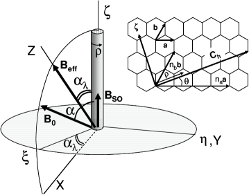
Figure 1: Reciprocal positions of CNT and coordinate systems. Insert: the lattice structure of graphene.

We begin with a few essential definitions concerning CNTs Ando05 . The CNT is conveniently imagined as a spiral graphite sheet (graphene) rolled along the chiral vector $\mathbf{C}_{h}$ (see Fig. 1). Here $\mathbf{C}_{h}=n_{a}\mathbf{a}+n_{b}\mathbf{b}$, where $\mathbf{a}=a(1,0)$ and $\mathbf{b}=a(1/2,\sqrt{3}/2)$ are the graphene lattice unit vectors with $a=0.246$ nm and $n_{a}$ and $n_{b}$ are integers, which characterize the geometry of a particular CNT. The slope of $\mathbf{C}_{h}$ is defined by $\tan\theta=\sqrt{3}n_{b}/(2n_{a}+n_{b})$ and the diameter of the CNT is given by $d=\left|\mathbf{C}_{h}\right|/\pi$. The energy band structure of graphene possesses two non-equivalent valleys with Dirac-like dispersion law in the vicinity of Fermi level Slonczewski57 . They are located at the $K=\frac{2\pi}{3a}\left(1,\sqrt{3}\right)$ and $K^{\prime}=\frac{2\pi}{3a}\left(-1,\sqrt{3}\right)$ corner points of the first Brillouin zone, which will be labeled by $\lambda=1,-1$ respectively.

The graphene two-valley band structure projects onto the CNT one so that in the vicinity of each valley the $kP$ Hamiltonian takes the form $H_{\lambda}=\hbar v_{F}(\lambda\varkappa_{m}\widehat{\sigma}_{1}+k\widehat{\sigma}_{2})$ Ando05 where the Fermi velocity is $v_{F}=8\cdot 10^{7}$ cm/s and Pauli  matrixes $\widehat{\sigma}_{1}$ and $\widehat{\sigma}_{2}$ are defined over the sublattice electronic states A and B. The wave vector $\mathbf{k}$ with respect to $K$ ($\lambda=1$) or $K^{\prime}$ ($\lambda=-1$) point is directed along the principal axis $\zeta$ of CNT. The rolling along the perpendicular direction $\rho$ (Fig. 1) imposes a quantization of the electron momentum in circumcircular direction fixing the wave numbers $\varkappa_{m}=2(m-\lambda\nu/3)/d$ with integer magnetic quantum number $m$ and $\nu$ (from the set 1, 0, -1) so that $2n_{a}+n_{b}+\nu$ becomes divisible by 3. If the CNT is subjected to a magnetic field $\mathbf{B}_{0}$ the Aharonov-Bohm magnetic flux passing through the CNT cross section $\phi_{AB}=B_{0}\cos\alpha\ \pi d^{2}/4$ modifies the quantization condition Ando05 ,

$$\varkappa_{m,\lambda}=2(m-\lambda\nu/3+\phi_{AB}/\phi_{0})/d,$$ (1)

where $\alpha$ is an angle between $\mathbf{B}_{0}$ and CNT axis, $\phi_{0}=2\pi\hbar c/\left|q_{0}\right|$ is the flux quantum, $q_{0}$ the electron charge.

The eigenvalues of Hamiltonian $H_{\lambda}$ describe the CNT electronic spectrum without spin structure,

$$\varepsilon_{k,m,\lambda}=\pm\hbar v_{F}\sqrt{\varkappa_{m,\lambda}^{2}+k^{2}},$$ (2)

where + (-) corresponds to the conduction (valence) band. The CNTs with $\nu=\pm 1$ possess the semiconducting spectrum, with bandgap $E_{g}=4\hbar v_{F}/3d$ even at zero magnetic field, with potential applications in spintronics Cottet06 . We assume $\nu=1$ in further numerical calculations.

When a spin-orbital interaction is incorporated in the Hamiltonian $H_{\lambda}$, the SOI mediated by CNT curvature which takes the simplest form in CNT co-ordinates $\xi$, $\eta$, $\zeta$ (Fig. 1) as:

$$H_{SO}=\Delta_{0}\lambda\widehat{\sigma}_{0}2S_{\zeta}+\Delta_{1}\lambda\widehat{\sigma}_{1}2S_{\zeta}-i\Delta_{2}\widehat{\sigma}_{2}(S_{+}e^{i\varphi}-S_{-}e^{-i\varphi}),$$ (3)

where $\widehat{\sigma}_{0}$ is $2\times 2$ identical matrix, $S_{\pm}=S_{\xi}\pm iS_{\eta}$, $\varphi=2\rho/d$, $0<\rho<\left|\mathbf{C}_{h}\right|$. In (3) the spin-orbital constants are proportional to CNT curvature, $\Delta_{0}=(\delta_{0}/d)\cos 3\theta$ , $\Delta_{1,2}=\delta_{1,2}/d$ where the parameter $\delta_{1}=-0.19$ meV$\cdot$nm has been measured comm1 and the ratios $\delta_{0}/\delta_{1}=4.5$ and $\delta_{2}/\delta_{1}=-1.4$ can be estimated theoretically Jeong09 ; Ando00 ; Brataas06 . The $\Delta_{0}$ depends on CNT chirality so that $\Delta_{0}$ is maximum in zigzag CNTs ($\theta=0$) and minimum $(\Delta_{0}=0$) in armchair ones ($\theta=\pi/6$) Jeong09 .

These estimates show that the SOI may be treated as a perturbation for actual electronic energies, i.e., $\left|\Delta_{i}\right|\ll\left|\varepsilon_{k,m,\lambda}\right|$. In the first order, the quantum averaging of the $H_{SO}$ on the eigenvectors $\left|k,m,\lambda\right\rangle$ of Hamiltonian $H_{\lambda}$ gives rise to the reduced Hamiltonian of SOI $H_{SO}^{\prime}$ of electron spin energy in an effective field $\mathbf{B}_{SO}^{\prime}$ directed along the principal axis $\zeta$ of the CNT, $H_{SO}^{\prime}=g\mu_{B}B_{SO}^{\prime}S_{\zeta}$, where $g\mu_{B}B_{SO}^{\prime}=2\lambda(\Delta_{0}+\Delta_{1}\sigma_{1})$. We take into account that $\left\langle k,m,\lambda\left|\widehat{\sigma}_{0}\right|k,m,\lambda\right\rangle=1$, $\left\langle k,m,\lambda\left|\widehat{\sigma}_{2}e^{\pm i\varphi}\right|k,m,\lambda\right\rangle=0$ and

$$\sigma_{1}=\left\langle k,m,\lambda\left|\widehat{\sigma}_{1}\right|k,m,\lambda\right\rangle=\mp\frac{\lambda\varkappa_{m,\lambda}}{\sqrt{k^{2}+\varkappa_{m}^{2}}}.$$ (4)

Here $\mp$ in Eq. (4) corresponds to conduction (valence) band.

An important issue of Eq. (4) is the dependence of $\mathbf{B}_{SO}^{\prime}(\sigma_{1})$ on $k$ i.e. electronic energy [eq. (2)]. This effect can be understood as a result of diminishing of electron velocity $v_{\perp}$ in the $\rho$-direction with increasing $\ k_{\parallel}$ along the CNT axis under constant total electron velocity $v_{F}$, i.e. $v_{\perp}/v_{F}=k_{\perp}/\left|\mathbf{k}\right|=k_{\perp}/\sqrt{k_{\perp}^{2}+k_{\parallel}^{2}}$ that appears as a factor in Eq. (4) at $k_{\parallel}=k$ and $k_{\perp}=\varkappa_{m,\lambda}$.

It is convenient to introduce the mean values $\left\langle\sigma_{1}\right\rangle=\sum\nolimits_{m}\int\sigma_{1}f(\varepsilon_{k,m,\lambda})dk\diagup\sum\nolimits_{m}\int f(\varepsilon_{k,m,\lambda})dk$ and $B_{SO}=\left\langle B_{SO}^{\prime}\right\rangle=2\lambda(\Delta_{0}+\Delta_{1}\left\langle\sigma_{1}\right\rangle)/g\mu_{B}$, where $f(\varepsilon_{k,m,\lambda})$ is a thermal population factor for electron with energy $\varepsilon_{k,m,\lambda}$. Correspondingly, the SOI can be separated into a steady part $g\mu_{B}B_{SO}S_{\zeta}$ and a fluctuating one $\Omega S_{\zeta}$ with

$$\Omega=2\Delta_{1}\lambda\left(\sigma_{1}-\left\langle\sigma_{1}\right\rangle\right).$$ (5)

Fluctuations in $k$ lead to fluctuations of the effective spin-orbital field and serve as a mechanism of spin relaxation in CNTs. Our analysis centers on the efficiency of this mechanism for CNTs in the presence of an external magnetic field $\mathbf{B}_{0}$. This supplements the Hamiltonian $H_{SO}$ with a Zeeman interaction $H_{Z}=g\mu_{B}\mathbf{B}_{0}\mathbf{S}$. The joint action determines a spin energy $g\mu_{B}\mathbf{B}_{eff}\mathbf{S}$ in an effective field $\mathbf{B}_{eff}=\mathbf{B}_{SO}+\mathbf{B}_{0}$.

In the reference frame ($\xi$, $\eta$, $\zeta$), the Zeeman Hamiltonian takes the form $H_{Z}=\hbar\omega_{Z}(\sin\alpha\ S_{\xi}+\cos\alpha\ S_{\zeta})$, $\hbar\omega_{Z}=g\mu_{B}B_{0}$ ($g=2$ and $\mu_{B}$ is the Bohr magneton) so that the frequency of spin precession $\omega_{\lambda}=g\mu_{B}B_{eff}/\hbar$ in a total effective field $\mathbf{B}_{eff}$ is Churchill09

$$\omega_{\lambda}=\sqrt{(\omega_{Z}\sin\alpha)^{2}+\left[\omega_{Z}\cos\alpha+2\lambda(\Delta_{0}+\Delta_{1}\left\langle\sigma_{1}\right\rangle)/\hbar\right]^{2}}.$$ (6)

Spin relaxation is conveniently described in other co-ordinates $X$, $Y$ and $Z$, where $Z$ is a spin quantization axis defined by the $\mathbf{B}_{eff}$. Correspondingly, evolution of $S_{Z}$ and $S_{X}$, $S_{Y}$ correlates with longitudinal (spin-flip) and transversal (phase) spin relaxation. The angle $\alpha_{\lambda}$ ($0\leq\alpha_{\lambda}\leq\pi$) of $\mathbf{B}_{eff}$ slope to CNT axis defines

$$\cos\alpha_{\lambda}=[\hbar\omega_{Z}\cos\alpha+2\lambda(\Delta_{0}+\Delta_{1}\left\langle\sigma_{1}\right\rangle)]\diagup\hbar\omega_{\lambda}.$$ (7)

In a second quantization representation, the operator of fluctuating field takes the form $\Omega=\sum\nolimits_{k,m}\mathbf{b}(k,m)n_{k,m}$, $n_{k,m}=a_{k,m}^{\dagger}a_{k,m}$, where $a_{k,m}^{\dagger}$ and $a_{k,m}$ are creation and annihilation operators and the vector $\mathbf{b}(k,m)=2\Delta_{1}\lambda\left(\sigma_{1}-\left\langle\sigma_{1}\right\rangle\right)(-\sin\alpha_{\lambda},0,\cos\alpha_{\lambda})$ is expressed in co-ordinates X, Y, and Z.

Assuming a short correlation time $\tau_{p}$ for the electronic correlation function $\left\langle n_{k,m}(t)n_{k,m}\right\rangle$ in comparison with the spin relaxation time $\tau_{S}$, one can use the Markovian equations of spin evolution in form of expanded Bloch equations in which the spin mean values $\left\langle\mathbf{S}\right\rangle=Tr\widehat{\rho}(t)\mathbf{S}$ ($\widehat{\rho}(t)$ is a density matrix SSK ). Then the spin polarization deviation from thermal equilibrium becomes $\mathbf{P}=2(\left\langle\mathbf{S}\right\rangle-\left\langle\mathbf{S}\right\rangle_{\infty})$ , where $2\left\langle\mathbf{S}\right\rangle_{\infty}\mathbf{=}2\lim_{t\rightarrow\infty}\left\langle\mathbf{S}\right\rangle=\mathbf{(}0,0,-\tan\hbar\omega_{\lambda}/2k_{B}T\mathbf{)}$. These equations take the simplest form in the $X$, $Y\,$,$\ Z$ coordinate system:

$$\frac{d\mathbf{P}_{\lambda}}{dt}=\left(\widehat{\mathbf{\omega}}_{\lambda}-\widehat{\mathbf{\Gamma}}_{\lambda}\right)\mathbf{P}_{\lambda},$$ (8)

where the $3\times 3$ matrix $\widehat{\mathbf{\omega}}_{\lambda}$ represents the cross product of $\overrightarrow{\mathbf{\omega}}_{\lambda}\mathbf{=(}0,0,\omega_{\lambda}\mathbf{)}$, $\widehat{\mathbf{\omega}}_{\lambda}\mathbf{P}_{\lambda}=\overrightarrow{\mathbf{\omega}}_{\lambda}\mathbf{\times P}_{\lambda}$. Thus, $\widehat{\mathbf{\omega}}_{\lambda}$ includes only two non-zero matrix elements $\omega_{YX}=-\omega_{XY}=\omega_{\lambda}$, and $\widehat{\mathbf{\omega}}_{\lambda}\mathbf{S}_{0}=\mathbf{0}$. In this case the matrix of relaxation parameters can be reduced to

$$\widehat{\mathbf{\Gamma}}_{\lambda}\mathbf{=}\left(\begin{array}[]{ccc}R_{XX}^{(\lambda)}&0&R_{XZ}^{(\lambda)}\\ 0&R_{YY}^{(\lambda)}&0\\ R_{XZ}^{(\lambda)}&0&R_{ZZ}^{(\lambda)}\end{array}\right).$$ (9)

The low symmetry of the CNT affected by an arbitrary magnetic field produces multiple spin-relaxation parameters $R_{\mu,\nu}^{(\lambda)}$, $\mu,\nu=X$, $Y$, $Z$ [four in the case of Eq. (9)], which cannot be immediately associated with longitudinal or transversal spin relaxation rates. In the most general form they can be represented in terms of Fourier transformation of correlation functions $\left\langle\Omega_{\mu}(t)\Omega_{\nu}\right\rangle_{\omega}$ at frequency $\omega=\omega_{\lambda}$. For spin precession in a fluctuating field they can be evaluated in an approximation of a momentum relaxation time $\tau_{k}$ Pikus ; SSK that assumes explicit knowledge of the $\tau_{k}$ dependence on $k$. Instead, we use the average value $\tau_{p}^{-1}=\left\langle\tau_{k}^{-1}\right\rangle$ to evaluate the spin-relaxation characteristics while the specific dependence of $\tau_{k}$ on $k$ can be taken into account by introducing the numerical factor, which is about $Q_{1}\simeq 1.5\div 3$ Pikus . Based on a recent study Habenicht08  we assign $\tau_{p}=1$ ps and assume $Q_{1}=2$ for further numerical calculations.

Applying these approximations we find

$$R_{XX}^{(\lambda)} = \cos^{2}\alpha_{\lambda}\frac{(2\Delta_{1})^{2}\tau_{p}}{\hbar^{2}}Q_{1}\Delta\sigma_{1}^{2};$$

$$R_{ZZ}^{(\lambda)} = \sin^{2}\alpha_{\lambda}\frac{(2\Delta_{1})^{2}\tau_{p}}{\hbar^{2}(\omega_{S}^{2}\tau_{p}^{2}+1)}Q_{1}\Delta\sigma_{1}^{2};$$ (10)

$$R_{YY}^{(\lambda)} = R_{XX}^{(\lambda)}+R_{ZZ}^{(\lambda)};$$

$$R_{XZ}^{(\lambda)} = \frac{R_{XX}^{(\lambda)}}{2}\tan\alpha_{\lambda}+\frac{R_{ZZ}^{(\lambda)}}{2}\cot\alpha_{\lambda},$$

where $\Delta\sigma_{1}^{2}=\left\langle\sigma_{1}^{2}\right\rangle-\left\langle\sigma_{1}\right\rangle^{2}$ critically depends on the temperature so that $\Delta\sigma_{1}\rightarrow 0$ at $T\rightarrow 0$. Results of calculations of the relaxation rate parameters [Eq. (10]) as a function of temperature, magnetic field strength and direction, and CNT diameter are presented in Fig. 2. It can be noticed that there is not a single $R_{\mu\nu}^{(\lambda)}$, which significantly dominates over all ranges of $T$, $\mathbf{B}_{0}$, and $d$. Thus the full set of $R_{\mu\nu}^{(\lambda)}$ is required to describe spin relaxation in CNTs. All $R_{\mu\nu}^{(\lambda)}$ are strongly depended on temperature that controls energy dispersion. Moreover, the relaxation rate decreases with an increase of CNT diameter due to SOI reduction with decreasing curvature. The non-monotonic dependence on the external magnetic field strength and its direction depends upon the interplay between $\mathbf{B}_{SO}$ and $\mathbf{B}_{0}$ that leads to suppression of $R_{ZZ}^{(\lambda)}$ and $R_{XZ}^{(\lambda)}$ when $\alpha\rightarrow 0$ or $B_{0}\rightarrow 0$.

Examples of numerical solutions to Eqs. (8,9,10) are shown in Fig. 3. In particular, interference of spin polarizations from the two non-equivalent valleys can lead to the oscillation amplitude beating shown in Fig. 3(a) where beats alternate with nodes in   90 ps. When the magnetic field is perpendicular to the CNT axis ($\alpha=90^{\circ}$), a fast polarization damping is found for longitudinal ($\tau_{s}\simeq 150$ ps) and transversal ($\tau_{s}\simeq 110$ ps) spin polarizations as seen in Fig. 3(b). A greater variation of spin relaxation exists in CNTs with different chirality placed in an arbitrary directed magnetic field.

The developed theory can be applied to MR measurements which are usually carried out on a CNT with weak contacts to source/drain ferromagnets. Electron undergo multiple reflections from the contacts before exiting. In such a case the output signal depends on both spin relaxation time $\tau_{s}$ and electron dwell time $\tau_{d}$ Hueso07 . The experimental setup also provides for electron injection into the CNT with spin polarization along magnetization $\mathbf{M}_{S}$ of ferromagnetic source and spin detection with a ferromagnetic drain polarized in either the same direction $\mathbf{M}_{D}=\mathbf{M}_{S}$ or the opposite one, $\mathbf{M}_{D}^{\prime}=-\mathbf{M}_{S}$. Spin dependent output from each valley $\Delta I_{\lambda}$ is proportional to difference $\mathbf{m}\overline{\mathbf{P}}_{\lambda}-\mathbf{m}^{\prime}\overline{\mathbf{P}}_{\lambda}=2\mathbf{m}\overline{\mathbf{P}}_{\lambda}$ ($\mathbf{m}=\mathbf{M}_{D}/\left|\mathbf{M}_{D}\right|$, $\mathbf{m}^{\prime}=-\mathbf{m}$) where the spin polarization is averaged over $\tau_{d}$ ( $\overline{\mathbf{P}}_{\lambda}=\frac{1}{\tau_{d}}\int\nolimits_{0}^{\infty}\mathbf{P}_{\lambda}(t)e^{-t/\tau_{d}}dt$) provided that $\tau_{d}$ is longer than electron drift from source to drain. $\overline{\mathbf{P}}_{\lambda}$ can be found from Eq. (8) by multiplication with $e^{-t/\tau_{d}}$ and subsequent integration over $t$. Assuming that the rate of intervalley transitions is less than $R_{d}=1/\tau_{d}$ , the total spin-depended output can be expressed as $\sum\nolimits_{\lambda}\Delta I_{\lambda}/2=F_{s}R_{d}$, where

$$F_{s}=c\mathbf{m}\sum\nolimits_{\lambda}(\widehat{\mathbf{\Gamma}}_{\lambda}+\widehat{\mathbf{I}}R_{d}-\widehat{\mathbf{\omega}}_{\lambda})^{-1}\mathbf{m}.$$ (11)

Here $c$ is a dimensional constant and $\widehat{\mathbf{I}}$ is the identity $3\times 3$ matrix. In the case of $\omega_{\lambda}=0,$ $\widehat{\mathbf{\Gamma}}_{\lambda}=\widehat{\mathbf{I}}/\tau_{s}$, Eq. (11) reduces to $F_{s}=c/(\tau_{d}^{-1}+\tau_{s}^{-1})$ which is in agreement with previous calculations Hueso07 . In more general situations, the following relation holds

$$\tau_{s}=-\lim_{R_{d}\rightarrow 0}\frac{d\ln F_{s}}{dR_{d}}.$$ (12)

If $\omega_{\lambda}\gg R_{\mu\nu}^{(\lambda)}\equiv 1/\tau_{\mu\nu}^{(\lambda)}$, the last equation leads to $\tau_{s}=\sum\nolimits_{\lambda}\tau_{ZZ}^{(\lambda)2}\diagup\sum\nolimits_{\lambda}\tau_{ZZ}^{(\lambda)}$. Thus, only longitudinal spin relaxation (i.e. spin-flip) can control the magnetoresistance measurements in a CNT at strong magnetic field. In Fig. 3c the calculated dependence of $\tau_{s}$ on the chiral angle $\theta$ of the CNT is displayed. For example, $\tau_{s}\simeq 220$ ps at $T=$300 K, for the case of $B_{0}=$0.5 T, $d=$2 nm, $\mathbf{m}\parallel\mathbf{B}_{0}$ $\alpha=90^{\circ}$ and $\theta=26^{\circ}$.

However spin relaxation is suppressed at small values of $\alpha$. The experimental setup treated in Ref. Hueso07 displays a small deviation of the magnetization direction from the CNT axis, with $\alpha\simeq 10^{\circ}$. For such a case and with $T=120$ K, $B_{0}=$0.1 T and $d=$ 10 nm Eq. (12) predicts $\tau_{s}\simeq 69$ ns which approaches the measured $\tau_{s}=$30 ns. This results indicates the high efficiency of the spin relaxation mechanism even through small symmetry breaking in the design of realistic devices.

In conclusion, we show that the fluctuations of curvature-induced spin-orbital interaction that are associated with electron random motion in CNTs is responsible for the short spin relaxation. If a magnetic field preserves the uniaxial symmetry of CNT, the spin-flip relaxation is suppressed. However a small asymmetry may lead to visible manifestations of this precession change. These issues may stimulate further experiments to determine the optimal conditions for room temperature CNT spintronic device applications.

This work was supported in part by the US Army Research Office, NSF, and the FCRP Center on Functional Engineered Nano Architectonics (FENA).

Figure 2: $R_{XX}$ (solid lines), $R_{ZZ}$ (dashed lines) and $R_{XZ}$ (doted lines) calculated as an average over valleys and the functions of (a) temperature [$(n_{a},n_{b})=(15,14)$, $B_{0}=2$ T, $\alpha=\pi/2$], (b) magnetic field strength [$(n_{a},n_{b})=(15,14)$, $T=300$ K, $\alpha=\pi/2$ ], (c) the nanotube diameter [$T=300$ K, $B_{0}=2$ T, $\alpha=\pi/2$, $\theta=27^{\circ}$] and (d) the angle $\alpha$ between external magnetic field direction and CNT axis [$(n_{a},n_{b})=(17,13)$, $T=300$ K, $B_{0}=2$ T]. For convenience the right parts of the graphs are scaled in nanoseconds as a reciprocal values.

Figure 3: (a) $(n_{a},n_{b})=(15,14)$, $B_{0}=0.2$ T and $\alpha=30^{\circ}$ (b) $(n_{a},n_{b})=(17,13)$, $B_{0}=0.05$ T and $\alpha=90^{\circ}$. Solid (dashed) lines corresponds to transversal $P_{\xi}$ (longitudinal $P_{\zeta}$) spin polarization. Thin horizontal line cuts the polarization curves at the level $1/e$, which indicates the relaxation times 110 ps and 150 ps for $P_{\xi}$ and $P_{\zeta}$. Insert (c) displays the dependence of relaxation time $\tau_{S}$ on chiral angle calculated with Eq. (12) under constant $d=10$ nm, $B_{0}=2$ T and $\alpha=90^{\circ}$.

References

• (1) A. Cottet et al., Semicond. Sci. Technol. 21, S78 (2006).
• (2) A. Fert et al., IEEE Trans. Electron Dev. 54, 921 (2007).
• (3) K. Tsukagoshi, W. B. Alphenaar, and H. Ago, Nature 401, 572 (1999).
• (4) S. Sahoo et al., Nature Phys. 1, 99 (2005).
• (5) P. Petit et al., Phys. Rev. B 56, 9275 (1997).
• (6) L. E. Hueso et al., Nature 445, 410 (2007).
• (7) Y. G. Semenov, K. W. Kim, and G. J. Iafrate, Phys. Rev. B 75, 045429 (2007).
• (8) H. O. H. Churchill et al., Nature Phys. 5, 321 (2009).
• (9) J. Serrano, M. Cardona, and J. Ruff, Solid State Commun. 113, 411 (2000).
• (10) D. Huertas-Hernando, F. Guennea, and A. Brataas, Phys. Rev. B 74, 155426 (2006).
• (11) T. Ando, J. Phys. Soc. Japan 69, 1757 (2000).
• (12) J.-S. Jeong and H.-W. Lee, Phys. Rev. B 80, 075409 (2009).
• (13) W. Izumida, K. Sato, and R. Satoito, J. Phys. Soc. Japan 78, 074707 (2009).
• (14) L. Chico, M. P. LΓ³pez-Sancho, and M. C. MuΓ±oz, Phys. Rev. B 79, 235423 (2009).
• (15) F. Kuemmeth et al., Nature 452, 448 (2008).
• (16) D. V. Bulaev, B. Trauzettel, and D. Loss, Phys. Rev. B 77, 235301 (2008).
• (17) T. Ando, J. Phys. Soc. Japan 74, 777 (2005).
• (18) J. C. Slonczewski and P. R. Weiss, Phys. Rev. 109, 272 (1958).
• (19) Evaluating the $\Delta_{1}$ in Ref. Kuemmeth08 , the contribution of first term $\sim\Delta_{0}$ in Eq.Β (3) was not taken into account. It does not matter if $\cos 3\theta\approx 0$; we suppose that this was the case for the actual CNT in Ref.Β Kuemmeth08, .
• (20) H. O. H. Churchill et al., Phys. Rev. Lett. 102, 166802 (2009).
• (21) Y. G. Semenov, Phys. Rev. B 67, 115319 (2003); Y. G. Semenov and K. W. Kim, ibid 75, 195342 (2007).
• (22) G. E. Pikus and A. N. Titkov, in Optical Orientation, Ed. F. Meier and B. P. Zakharchenia (Elsevier, Amsterdam, 1984), Chap. 3.
• (23) B. F. Habenicht, S. V. Kilina, and O. V. Prezhdo, Pure Appl. Chem. 80, 1433 (2008).
Refer to caption