Classifying Network Data with Deep Kernel Machines

Abstract

Inspired by a growing interest in analyzing network data, we study the problem of node classification on graphs, focusing on approaches based on kernel machines. Conventionally, kernel machines are linear classifiers in the implicit feature space. We argue that linear classification in the feature space of kernels commonly used for graphs is often not enough to produce good results. When this is the case, one naturally considers nonlinear classifiers in the feature space. We show that repeating this process produces something we call “deep kernel machines.” We provide some examples where deep kernel machines can make a big difference in classification performance, and point out some connections to various recent literature on deep architectures in artificial intelligence and machine learning.

Key Words: deep architecture; diffusion kernel; kernel density estimation; nearest centroid; social network; support vector machine.

1 Introduction

Given a graph, $\mathcal{G}$, let $V(\mathcal{G})=\{\mathbf{v}_{1},\mathbf{v}_{2},...,\mathbf{v}_{n}\}$ denote its set of vertices (nodes). Associated with each node $\mathbf{v}_{i}$ is a class label, say $y_{i}\in\{1,2,...,C\}$. A small number of these labels are known; others are unknown. We use the notation

$$V_{obs}(\mathcal{G})=\{\mathbf{v}_{i}\in V(\mathcal{G}):y_{i}\mbox{ observed}\}\quad\mbox{and}\quad V_{miss}(\mathcal{G})=\{\mathbf{v}_{i}\in V(\mathcal{G}):y_{i}\mbox{ missing}\}$$

to denote subsets of nodes whose labels are known and unknown, respectively. The problem that we study in this article is that of predicting the unknown labels based on how the nodes are connected to each other.

For example, $\mathcal{G}$ may be a protein interaction network. Some proteins are known to be associated with certain biological functions (e.g., cell communication), and we may be interested in predicting which of the remaining proteins are also associated. Another example of $\mathcal{G}$ is a social network, where the nodes are individuals. Some individuals are known to be involved with certain activities (e.g., belonging to a certain club, or interested in certain products), and we may wish to assess the likelihood that the remaining individuals are also involved. For simplicity, we will assume $C=2$, i.e., there are only two classes, but our ideas also apply when $C>2$.

We develop something we call “deep kernel machines” (DKMs) on graphs. Though we focus on the problem of node classification on graphs, it will become clear by the end of this article (Section 5) that the idea of DKMs does not really depend on the graph structure of the data. The main reasons why we choose to start with the node classification problem on graphs are: (a) it is a relatively new problem and not as widely studied as some of the more conventional classification problems (Kolaczyk 2009); and (b) it is a problem for which kernel machines are particularly well suited (Shawe-Taylor and Cristianini 2004). Experiments with data structures other than graphs will be left as future work.

2 Kernel machines and graphs

Lately, largely due to support vector machines (see, e.g., Vapnik 1995; Cristianini and Shawe-Taylor 2000), kernel machines have become very popular in machine learning (Shawe-Taylor and Cristianini 2004; Bishop 2006). Typically, a kernel machine has the form,

$$f(\mathbf{v})=\alpha_{0}+\sum_{\mathbf{v}_{i}\in V_{obs}(\mathcal{G})}\alpha_{i}\mathbf{K}(\mathbf{v},\mathbf{v}_{i}),$$ (1)

where $\mathbf{K}(\cdot,\cdot)$ is a kernel function, and the coefficient $\alpha_{i}$ often depends on the class label $y_{i}$.

A support vector machine (SVM) is sometimes called a sparse kernel machine because the optimization problem it solves will cause many of the $\alpha_{i}$’s to be $0$. As a result, the decision function (1) depends only on those observations $(\mathbf{v}_{i},y_{i})$ with $\alpha_{i}>0$, and hence the name “sparse.” In order to crystalize the gist of our ideas, we shall mostly work with a much simpler kernel machine (Section 2.1), but other kernel machines such as SVMs also can be used.

As noted by Shawe-Taylor and Cristianini (2004), kernel machines are particularly well suited to analyze non-vectorial data such as graphs. Before we talk about kernels on graphs, a few graph-theoretic concepts are needed. The adjacency matrix, $\mathbf{A}_{\mathcal{G}}$, for graph $\mathcal{G}$ is defined as

$$\mathbf{A}_{\mathcal{G}}(i,j)=\begin{cases}1,&\mbox{if there is an edge between $\mathbf{v}_{i}$ and $\mathbf{v}_{j}$};\\ 0,&\mbox{if not}.\end{cases}$$

Let

$$d_{i}=\sum_{j\neq i}\mathbf{A}_{\mathcal{G}}(i,j)$$

be the degree of node $\mathbf{v}_{i}$, or simply the number of nodes it is adjacent to. The graph Laplacian matrix $\mathbf{L}_{\mathcal{G}}$ for $\mathcal{G}$ is defined by

$$\mathbf{L}_{\mathcal{G}}=\mathbf{D}_{\mathcal{G}}-\mathbf{A}_{\mathcal{G}},\quad\mbox{where}\quad\mathbf{D}_{\mathcal{G}}=\mbox{diag}\{d_{1},d_{2},...,d_{n}\}.$$

In other words,

$$\mathbf{L}_{\mathcal{G}}(i,j)=\begin{cases}d_{i},&\mbox{if }i=j;\\ -\mathbf{A}_{\mathcal{G}}(i,j),&\mbox{if }i\neq j.\end{cases}$$

With these basic notions, we are now ready to talk about kernels on graphs. For graph data, one often uses a so-called diffusion kernel (Lafferty and Lebanon 2005), defined as

$$\mathbf{K}_{\mathcal{G}}=\mbox{exp}(-\beta\mathbf{L}_{\mathcal{G}})=\sum_{m=0}^{\infty}\frac{(-\beta)^{m}}{m!}\mathbf{L}_{\mathcal{G}}^{m},$$ (2)

where $\beta>0$ is a tuning parameter. The meaning and intuition behind the diffusion kernel require a relatively long explanation, which we won’t go into. Roughly speaking, to measure the similarity between $\mathbf{v}_{i}$ and $\mathbf{v}_{j}$, the diffusion kernel takes into account the number of paths of length $m$ between $\mathbf{v}_{i}$ and $\mathbf{v}_{j}$, for all $m$, and gives shorter paths more weight (e.g., Kolaczyk 2009, Section 8.4.2).

More generally, one is not required to use the adjacency matrix or the graph Laplacian to construct the diffusion kernel. Instead, a diffusion kernel (2) can be constructed as long as $\mathbf{L}_{\mathcal{G}}$ is a valid similarity matrix (see, e.g., Shawe-Taylor and Cristianini 2004); we will show an example below (Section 4.2).

To compute the diffusion kernel, let $\mathbf{L}_{\mathcal{G}}=\mathbf{U\Sigma}\mathbf{U}^{T}$ be the spectral decomposition of the Laplacian matrix, where $\mathbf{\Sigma}=\mbox{diag}(s_{m})$. Using the fact that $\mathbf{L}_{\mathcal{G}}^{m}$ has the same eigenvectors for all $m$, the diffusion kernel can be computed by

$$\mathbf{K}_{\mathcal{G}}=\mathbf{U}\mbox{diag}\left(e^{-\beta s_{m}}\right)\mathbf{U}^{T}.$$

We will use $\mathbf{K}_{\mathcal{G}}(i,j)$ and $\mathbf{K}_{\mathcal{G}}(\mathbf{v}_{i},\mathbf{v}_{j})$ interchangeably.

2.1 A simple kernel machine

Since $\mathbf{K}_{\mathcal{G}}(\mathbf{v}_{i},\mathbf{v}_{j})$ measures the similarity between nodes $\mathbf{v}_{i}$ and $\mathbf{v}_{j}$, to classify $\mathbf{v}_{0}\in V_{miss}(\mathcal{G})$ we can clearly use the function,

$$f_{\mathcal{G}}(\mathbf{v}_{0})\equiv\frac{1}{n_{1}}\sum_{\begin{subarray}{c}\mathbf{v}_{i}\in V_{obs}(\mathcal{G})\\ y_{i}={1}\end{subarray}}\mathbf{K}_{\mathcal{G}}\left(\mathbf{v}_{0},\mathbf{v}_{i}\right)-\frac{1}{n_{2}}\sum_{\begin{subarray}{c}\mathbf{v}_{i}\in V_{obs}(\mathcal{G})\\ y_{i}={2}\end{subarray}}\mathbf{K}_{\mathcal{G}}\left(\mathbf{v}_{0},\mathbf{v}_{i}\right),$$ (3)

where $n_{1}$ and $n_{2}$ are total number of nodes in $V_{obs}(\mathcal{G})$ with class label $1$ and $2$, respectively. For $\mathbf{v}_{0}$, this is simply the difference between its average similarity to class 1 and its average similarity to class 2. For example, we can classify $\mathbf{v}_{0}$ to the class which it is more similar to, i.e.,

$$\hat{y}_{0}=\begin{cases}1,&\mbox{if }f_{\mathcal{G}}(\mathbf{v}_{0})>c,\\ 2,&\mbox{if otherwise},\end{cases}$$ (4)

for some thresholding constant $c$. Below, we will sometimes drop the subscript “$\mathbf{v}_{i}\in V_{obs}(\mathcal{G})$” from the summation in (3).

It is easy to see that the function $f_{\mathcal{G}}(\mathbf{v}_{0})$ in (3) is of the general form (1), with $\alpha_{0}=0$, $\alpha_{i}=1/n_{1}$ or $-1/n_{2}$ depending on whether $y_{i}=1$ or 2, and $\mathbf{K}=\mathbf{K}_{\mathcal{G}}$. In other words, (3) is a simple kernel machine. We shall mostly work with this simple kernel machine because it can easily be constructed without invoking expensive optimization procedures in order to determine the coefficients, $\alpha_{0},\alpha_{1},\alpha_{2},...,\alpha_{n}$. A more sophisticated kernel machine such as the SVM, on the other hand, would require quadratic programming to find these coefficients. However, though we use (3) for convenience, we emphasize the framework we develop below does not preclude us from using other kernel machines such as SVMs.

3 Deep kernel machines on $\mathcal{G}$

A key idea behind kernel machines is that kernels can be regarded as calculating inner products in an implicit feature space, call it $\mathcal{F}$. That is,

$$\mathbf{K}_{\mathcal{G}}(\mathbf{v}_{i},\mathbf{v}_{j})=\langle\phi(\mathbf{v}_{i}),\phi(\mathbf{v}_{j})\rangle,\quad\mbox{where}\quad\phi:V(\mathcal{G})\mapsto\mathcal{F}.$$

This means the kernel $\mathbf{K}_{\mathcal{G}}$ necessarily induces a distance function in $\mathcal{F}$,

$$d_{\mathcal{F}}(\mathbf{v}_{i},\mathbf{v}_{j}) = \|\phi(\mathbf{v}_{i})-\phi(\mathbf{v}_{j})\|$$ (5)

$$= \sqrt{\langle\phi(\mathbf{v}_{i}),\phi(\mathbf{v}_{i})\rangle-2\langle\phi(\mathbf{v}_{i}),\phi(\mathbf{v}_{j})\rangle+\langle\phi(\mathbf{v}_{j}),\phi(\mathbf{v}_{j})\rangle}$$

$$= \sqrt{\mathbf{K}_{\mathcal{G}}(\mathbf{v}_{i},\mathbf{v}_{i})-2\mathbf{K}_{\mathcal{G}}(\mathbf{v}_{i},\mathbf{v}_{j})+\mathbf{K}_{\mathcal{G}}(\mathbf{v}_{j},\mathbf{v}_{j})}$$

3.1 Linear classification in $\mathcal{F}$

Using the distance $d_{\mathcal{F}}$ — more specificly the squared distance $d^{2}_{\mathcal{F}}$, the decision rule (4) is equivalent to nearest-centroid classification in the feature space $\mathcal{F}$. To see this, notice that

$$\frac{1}{n_{1}}\sum_{y_{i}=1}\phi(\mathbf{v}_{i})\quad\mbox{and}\quad\frac{1}{n_{2}}\sum_{y_{i}=2}\phi(\mathbf{v}_{i})$$

are class centroids in $\mathcal{F}$. Nearest-centroid classification simply declares $\hat{y}_{0}=1$ if $\mathbf{v}_{0}$ is closer to the centroid of class 1, i.e., if

$$\left\|\phi(\mathbf{v}_{0})-\frac{1}{n_{1}}\sum_{y_{i}=1}\phi(\mathbf{v}_{i})\right\|^{2}<\left\|\phi(\mathbf{v}_{0})-\frac{1}{n_{2}}\sum_{y_{i}=2}\phi(\mathbf{v}_{i})\right\|^{2}.$$

This is equivalent to

$$\left[\langle\phi(\mathbf{v}_{0}),\phi(\mathbf{v}_{0})\rangle-\frac{2}{n_{1}}\sum_{y_{i}=1}\langle\phi(\mathbf{v}_{i}),\phi(\mathbf{v}_{0})\rangle+\frac{1}{n_{1}^{2}}\sum_{y_{i},y_{j}=1}\langle\phi(\mathbf{v}_{i}),\phi(\mathbf{v}_{j})\rangle\right]\\ -\left[\langle\phi(\mathbf{v}_{0}),\phi(\mathbf{v}_{0})\rangle-\frac{2}{n_{2}}\sum_{y_{i}=2}\langle\phi(\mathbf{v}_{i}),\phi(\mathbf{v}_{0})\rangle+\frac{1}{n_{2}^{2}}\sum_{y_{i},y_{j}=2}\langle\phi(\mathbf{v}_{i}),\phi(\mathbf{v}_{j})\rangle\right]<0.$$

Cancelling out $\langle\phi(\mathbf{v}_{0}),\phi(\mathbf{v}_{0})\rangle$ and dividing by $-2$, we obtain

$$\frac{1}{n_{1}}\sum_{y_{i}=1}\mathbf{K}_{\mathcal{G}}\left(\mathbf{v}_{0},\mathbf{v}_{i}\right)-\frac{1}{n_{2}}\sum_{y_{i}=2}\mathbf{K}_{\mathcal{G}}\left(\mathbf{v}_{0},\mathbf{v}_{i}\right)-c(V_{obs}(\mathcal{G}))>0,$$

where

$$c(V_{obs}(\mathcal{G}))\equiv\frac{1}{2n_{1}^{2}}\sum_{y_{i},y_{j}=1}\mathbf{K}_{\mathcal{G}}(\mathbf{v}_{i},\mathbf{v}_{j})-\frac{1}{2n_{2}^{2}}\sum_{y_{i},y_{j}=2}\mathbf{K}_{\mathcal{G}}(\mathbf{v}_{i},\mathbf{v}_{j})$$

is a constant that depends only on $V_{obs}(\mathcal{G})$ and not on $\mathbf{v}_{0}$. Clearly, this is equivalent to (4).

Being equivalent to nearest-centroid classification, the kernel machine (3) is a linear classifier in the feature space $\mathcal{F}$. In fact, most kernel machines are linear in the feature space, including SVMs.

3.2 Nonlinear classification in $\mathcal{F}$

However, it is quite possible that a linear classifier in $\mathcal{F}$ is not sufficient; we will show some examples below (Section 4). But, in principle, there is nothing that prevents us from using other, more flexible classifiers in $\mathcal{F}$. For example, using the distance $d_{\mathcal{F}}$, we may consider a classifier based on kernel density estimates. Let

$$\hat{p}_{k}(\mathbf{v})=\frac{1}{n_{l}}\sum_{\begin{subarray}{c}\mathbf{v}_{i}\in V_{obs}(\mathcal{G})\\ y_{i}=k\end{subarray}}K_{h({\mathcal{F}})}\left(d_{\mathcal{F}}(\mathbf{v},\mathbf{v}_{i})\right)$$ (6)

be a kernel density estimate of the distribution for class $k$. Many kernel functions can be used for density estimation, e.g.,

$$K_{h({\mathcal{F}})}(d_{\mathcal{F}})=\frac{1}{\sqrt{2\pi}h({\mathcal{F}})}\mbox{exp}\left(-\frac{d_{\mathcal{F}}^{2}}{2h^{2}({\mathcal{F}})}\right),$$ (7)

where $h({\mathcal{F}})$ is a bandwidth parameter, which serves to scale the distance $d_{\mathcal{F}}$. We shall write

$$\mathbf{K}_{\mathcal{F}}(\mathbf{v}_{i},\mathbf{v}_{j}) \equiv K_{h({\mathcal{F}})}\left(d_{\mathcal{F}}(\mathbf{v}_{i},\mathbf{v}_{j})\right).$$ (8)

Using (7) for $K_{h({\mathcal{F}})}$, $\mathbf{K}_{\mathcal{F}}$ is nothing but the well-known radial-basis or Gaussian kernel, except it uses the distance function $d_{\mathcal{F}}$ rather than a distance defined on the original graph $\mathcal{G}$. Therefore, (6) is a density estimate in the space $\mathcal{F}$ rather than on the original graph $\mathcal{G}$. The subscript $\mathcal{F}$ and the notation $h(\mathcal{F})$ are used to emphasize this fact and to differentiate $\mathbf{K}_{\mathcal{F}}$ from $\mathbf{K}_{\mathcal{G}}$, the kernel on the original graph $\mathcal{G}$ that induced the space $\mathcal{F}$.

Based on the kernel density estimates in (6), for each $\mathbf{v}_{0}\in V_{miss}(\mathcal{G})$ we can predict its class label $\hat{y}_{0}$ depending on whether $\hat{p}_{1}(\mathbf{v}_{0})-\hat{p}_{2}(\mathbf{v}_{0})$ is positive or negative. In other words, the decision function is simply

$$f_{\mathcal{F}}(\mathbf{v}_{0})=\frac{1}{n_{1}}\sum_{\begin{subarray}{c}\mathbf{v}_{i}\in V_{obs}(\mathcal{G})\\ y_{i}={1}\end{subarray}}\mathbf{K}_{\mathcal{F}}\left(\mathbf{v}_{0},\mathbf{v}_{i}\right)-\frac{1}{n_{2}}\sum_{\begin{subarray}{c}\mathbf{v}_{i}\in V_{obs}(\mathcal{G})\\ y_{i}={2}\end{subarray}}\mathbf{K}_{\mathcal{F}}\left(\mathbf{v}_{0},\mathbf{v}_{i}\right).$$ (9)

It is easy to see that (9) is another kernel machine of the same form as (3); the only difference is that (9) uses the kernel $\mathbf{K}_{\mathcal{F}}$ whereas (3) uses the kernel $\mathbf{K}_{\mathcal{G}}$.

3.3 Deep kernel machines

Let us summarize what we have said so far. The space $\mathcal{F}$ is the implicit feature space for $\mathbf{K}_{\mathcal{G}}$. A kernel machine $f_{\mathcal{G}}$ (3) using the kernel $\mathbf{K}_{\mathcal{G}}$ is a linear classifier in $\mathcal{F}$. If linear classifiers are not sufficient in $\mathcal{F}$, we can relax linearity and choose to work with a nonlinear classifier, e.g., by constructing kernel density estimates in $\mathcal{F}$ via the implied distance metric $d_{\mathcal{F}}(\mathbf{v}_{i},\mathbf{v}_{j})$ — equation (5). This gives rise to a new kernel machine $f_{\mathcal{F}}$ (9), using the kernel $\mathbf{K}_{\mathcal{F}}(\mathbf{v}_{i},\mathbf{v}_{j})$ — equation (8). If we use (7) for kernel density estimation, the kernel updating formula from $\mathbf{K}_{\mathcal{G}}$ to $\mathbf{K}_{\mathcal{F}}$ is simply, putting (5), (7), and (8) together,

$$\mathbf{K}_{\mathcal{F}}(\mathbf{v}_{i},\mathbf{v}_{j}) = \frac{1}{\sqrt{2\pi}h({\mathcal{F}})}\mbox{exp}\left(-\frac{\mathbf{K}_{\mathcal{G}}(\mathbf{v}_{i},\mathbf{v}_{i})-2\mathbf{K}_{\mathcal{G}}(\mathbf{v}_{i},\mathbf{v}_{j})+\mathbf{K}_{\mathcal{G}}(\mathbf{v}_{j},\mathbf{v}_{j})}{2h^{2}({\mathcal{F}})}\right).$$ (10)

The choice of $h({\mathcal{F}})$ will be discussed below (Section 3.4).

However, there is no reason why the process must end here. The kernel $\mathbf{K}_{\mathcal{F}}$ has its implicit feature space as well; let’s call it $\mathcal{F}^{2}$. The kernel machine $f_{\mathcal{F}}$ (9) using the kernel $\mathbf{K}_{\mathcal{F}}$ is a linear classifier in $\mathcal{F}^{2}$. We can relax linearity in $\mathcal{F}^{2}$, if necessary, and choose to work with a nonlinear classifier, again, by constructing kernel density estimates in $\mathcal{F}^{2}$ via the implied distance metric,

$$d_{\mathcal{F}^{2}}(\mathbf{v}_{i},\mathbf{v}_{j})=\sqrt{\mathbf{K}_{\mathcal{F}}(\mathbf{v}_{i},\mathbf{v}_{i})-2\mathbf{K}_{\mathcal{F}}(\mathbf{v}_{i},\mathbf{v}_{j})+\mathbf{K}_{\mathcal{F}}(\mathbf{v}_{j},\mathbf{v}_{j})}.$$

By the same argument, this would give us yet another kernel machine, say $f_{\mathcal{F}^{2}}$, of exactly the same form as $f_{\mathcal{G}}$ (3) and $f_{\mathcal{F}}$ (9), except it would be using the kernel

$$\mathbf{K}_{\mathcal{F}^{2}}(\mathbf{v}_{i},\mathbf{v}_{j}) \equiv K_{h({\mathcal{F}^{2}})}\left(d_{\mathcal{F}^{2}}(\mathbf{v}_{i},\mathbf{v}_{j})\right)$$

$$= \frac{1}{\sqrt{2\pi}h({\mathcal{F}^{2}})}\mbox{exp}\left(-\frac{\mathbf{K}_{\mathcal{F}}(\mathbf{v}_{i},\mathbf{v}_{i})-2\mathbf{K}_{\mathcal{F}}(\mathbf{v}_{i},\mathbf{v}_{j})+\mathbf{K}_{\mathcal{F}}(\mathbf{v}_{j},\mathbf{v}_{j})}{2h^{2}({\mathcal{F}^{2}})}\right).$$

It is easy to see that this process can be repeated recursively (see Table 1). We refer to kernel machines generated by this recursive process as “deep kernel machines” (DKMs). The one using the original kernel $\mathbf{K}_{\mathcal{G}}$ is a referred to as a level-0 DKM; the one using the kernel $\mathbf{K}_{\mathcal{F}}$, a level-1 DKM; the one using the kernel $\mathbf{K}_{\mathcal{F}^{2}}$, a level-2 DKM; and so on. Notice that the DKM algorithm presented in Table 1 is slightly more general than what we have discussed above. In our discussion, we have focused on a specific base kernel machine (Section 2.1), but one can certainly use other base kernel machines, e.g., SVMs (see Section 4.4 below).

Table 1: Pseudo code for deep kernel machines (DKMs).

function BaseKernelMachine($\mathbf{K}$, $V_{obs}(\mathcal{G})$, $V_{miss}(\mathcal{G})$) for (every $\mathbf{v}\in V_{miss}(\mathcal{G})$) { $$f(\mathbf{v})=\alpha_{0}+\sum_{\mathbf{v}_{i}\in V_{obs}(\mathcal{G})}\alpha_{i}\mathbf{K}(\mathbf{v},\mathbf{v}_{i}),$$   e.g., $\alpha_{0}=0$, $\alpha_{i}=1/n_{1}$ if $y_{i}=1$ and $\alpha_{i}=-1/n_{2}$ if $y_{i}=2$. } return $f$; end function function GetKernel($\mathbf{K}_{\mathcal{G}}$, $level$) if ($level==0$) {    return $\mathbf{K}_{\mathcal{G}}$; } else {    compute $d_{\mathcal{F}}$ according to equation (5): $$d_{\mathcal{F}}(\mathbf{v}_{i},\mathbf{v}_{j})=\sqrt{\mathbf{K}_{\mathcal{G}}(\mathbf{v}_{i},\mathbf{v}_{i})-2\mathbf{K}_{\mathcal{G}}(\mathbf{v}_{i},\mathbf{v}_{j})+\mathbf{K}_{\mathcal{G}}(\mathbf{v}_{j},\mathbf{v}_{j})};$$    choose $h({\mathcal{F}})$ according to equation (11): $$h({\mathcal{F}})=\frac{1}{n^{2}}\underset{\mathbf{v}_{i},\mathbf{v}_{j}\in V_{obs}(\mathcal{G})}{\sum\sum}d_{\mathcal{F}}(\mathbf{v}_{i},\mathbf{v}_{j});$$    compute $\mathbf{K}_{\mathcal{F}}$ according to equations (8) and (7): $$\mathbf{K}_{\mathcal{F}}(\mathbf{v}_{i},\mathbf{v}_{j})=K_{h({\mathcal{F}})}\left(d_{\mathcal{F}}(\mathbf{v}_{i},\mathbf{v}_{j})\right);$$    return GetKernel($\mathbf{K}_{\mathcal{F}}$, $level-1$); } end function function DeepKernelMachine($\mathbf{K}_{\mathcal{G}}$, $V_{obs}(\mathcal{G})$, $V_{miss}(\mathcal{G})$, $level$) return BaseKernelMachine(GetKernel($\mathbf{K}_{\mathcal{G}}$, $level$), $V_{obs}(\mathcal{G})$, $V_{miss}(\mathcal{G})$); end function

3.4 A heuristic for choosing $h({\mathcal{F}})$

To carry out density estimation in $\mathcal{F}$, a bandwidth parameter $h({\mathcal{F}})$ must be specified; see (6) and (7). While users are certainly free to optimize this parameter in practice, this can be tedious for DKMs because, as we go from $\mathcal{G}$ to $\mathcal{F},\mathcal{F}^{2},\mathcal{F}^{3},...$, there is a bandwidth parameter for each space, $h(\mathcal{F}),h(\mathcal{F}^{2}),h(\mathcal{F}^{3}),...$, so a heuristic is desired. A reasonable heuristic is:

$$h({\mathcal{F}})=\frac{1}{n^{2}}\underset{\mathbf{v}_{i},\mathbf{v}_{j}\in V(\mathcal{G})}{\sum\sum}d_{\mathcal{F}}(\mathbf{v}_{i},\mathbf{v}_{j}).$$ (11)

That is, $h({\mathcal{F}})$ can be chosen to be the average pair-wise distance in the space of $\mathcal{F}$. We use this heuristic in all of our experiments below.

4 Experiments

In this section, we describe a few experiments and show that DKMs are useful.

4.1 Enron email data

In 2001, a large USA-based gas and electricity company named Enron was found guilty of serious accounting frauds, a case that caught worldwide attention. As part of the investigation, the US Federal Energy Regulatory Commission confiscated its corporate email database and made it publicly available. Preprocessed versions of these data can be obtained from http://cis.jhu.edu/~parky/Enron/enron.html. In particular, there is a $184\times 184$ adjacency matrix, $\mathbf{A}_{\mathcal{G}}$, that indicates whether there was email communication between any two of 184 unique email accounts. Our initial $\mathbf{K}_{\mathcal{G}}$ is simply a diffusion kernel (2) based on this adjacency matrix, but we removed two accounts that never sent an email to another account. The status of these 184 email account owners are also available, which we use to create two different classification tasks (see Table 2).

Table 2: Part of Enron email data used for tasks 1 and 2. We removed two accounts that never sent an email to another account.

Class Label Node Status $N$ Unbalanced Balanced CEO 5 1 1 President 5 1 1 Managing Director 6 1 1 Director 14 2 1 Vice President 30 2 1 Manager 16 2 1 Lawyer 1 2 1 Employee 40 2 2 Trader 11 2 2 Other 54 2 2 Total 182 16 vs 166 77 vs 105 (Task 1) (Task 2)

4.2 Lazega lawyer data

Lazega (2001) studied collaborative working relationships and social interactions among members of a New England law firm. There were 36 partners in the firm. The 36 partners were interviewed and asked to express their opinions on various issues regarding how the law firm should be managed. One of the issues had to do with workflow inside the firm (Lazega 2001, Chapter 8). Some favored the status quo ($y_{i}=1$) while others favored less flexible workflow ($y_{i}=2$). As our third classification task (see Table 3), we try to predict the partners’ position on this particular issue based on their social interactions and working relationships, e.g., whether any two partners worked together or considered themselves to be friends. Our initial $\mathbf{K}_{\mathcal{G}}$ is a diffusion kernel (2) based on a similarity (rather than adjacency) matrix $\mathbf{A}_{\mathcal{G}}$, defined as follows:

$$\mathbf{A}_{\mathcal{G}}(i,j)=0.5\times\mathbf{I}_{friends}(i,j)+0.5\times\mathbf{I}_{collaborated}(i,j),$$

where $\mathbf{I}_{friends}(i,j)=1$ if $\mathbf{v}_{i}$ and $\mathbf{v}_{j}$ were friends and $0$ if not; and likewise for $\mathbf{I}_{collaborated}(i,j)$.

Table 3: Part of Lazega lawyer data used for task 3.

Node Position $N$ Class Label Favors status quo 20 1 Favors less flexible workflow 16 2 Total 36 20 vs 16 (Task 3)

4.3 Performance measure

Classification task 1 (Table 2) is a highly unbalanced problem. For this task, we use the average precision (e.g., Zhu et al. 2006, Appendix A), or simply AP, to evaluate performance. The AP is a widely used criterion in the information retrieval community, and is particularly suitable for unbalanced classification problems. Classification tasks 2 and 3 (Tables 2 and 3) are relatively balanced problems. For these two tasks, we use the area under the receiver-operating characteristic (ROC) curve (Pepe 2003), or simply AUC (for “area under the curve”), to evaluate performance. The main reason for using the AUC and the AP (rather than, e.g., total misclassification error) is because they are not affected by the thresholding constant $c$ in equation (4). Table 4 summarizes the main features of the three tasks.

Table 4: Summary of classification tasks.

% Data Performance ($y_{i}=1$) Set $\mathbf{A}_{\mathcal{G}}$ Measure Task 1 8.8 Enron adjacency matrix AP Task 2 42.3 Enron adjacency matrix AUC Task 3 55.6 Lawyer custom similarity matrix AUC

4.4 Base kernel machines

We use two types of base kernel machines to run DKMs: the simple kernel machine (3) and the SVM. Both are linear in the feature space, but SVM directly goes after the optimal hyperplane. Notice that, to fit an SVM, one must specify the amount of penalty on the sum of slack variables, often called the “cost” parameter in most SVM packages. Every time an SVM is fitted, we simply choose the best “cost” parameter among a wide range of values:

$$10^{-5},10^{-4},10^{-3},10^{-2},0.05,0.1,0.5,1,2,5,10,50,100.$$

This gives the SVM an unfair advantage, but, since we are using SVMs as a benchmark, it is well understood that giving the benchmark an unfair advantage will only lead us to more conservative conclusions. In reality, this extra “cost” parameter in the SVM must be chosen by cross validation on $V_{obs}(\mathcal{G})$.

4.5 Results and conclusions

Figure 1 shows the average results over 25 random splits of $V(\mathcal{G})$ into $V_{obs}(\mathcal{G})$ and $V_{miss}(\mathcal{G})$. The random splits are stratified by class label so that the fraction of nodes belonging to each class is roughly the same on both $V_{obs}(\mathcal{G})$ and $V_{miss}(\mathcal{G})$. The main conclusions we can draw from Figure 1 are as follows:

• Though it goes directly after an “optimal” linear classifier, the SVM is not necessarily a better base kernel machine than a simple kernel machine such as (3). Both are linear in the feature space. It is more important to be in the “right” feature space than to use an “optimal” linear classifier. Using the “optimal” linear classifier in the “wrong” feature space is not going to give you good results. DKMs address this issue directly by providing a recursive algorithm to look for the “right” feature space.

• When the initial kernel $\mathbf{K}_{\mathcal{G}}$ is badly specified, e.g., if the tuning parameter $\beta$ is not well chosen for the underlying prediction task, DKMs can often boost up the performance significantly. This shows that DKMs have an attractive “automatic kernel correction” capability. When linear classification in the initial feature space $\mathbf{K}_{\mathcal{F}}$ is not enough to produce good results, it often pays to relax linearity and to go up to higher-level feature spaces. DKMs provide an automatic way to do so.

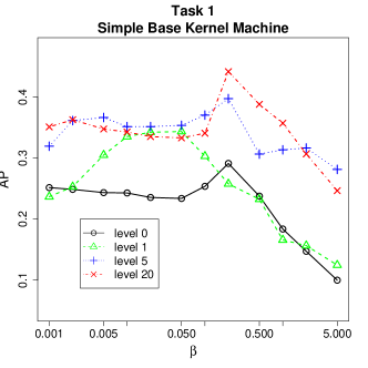
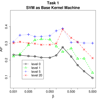
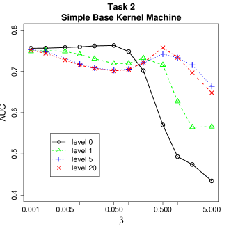
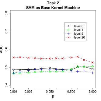
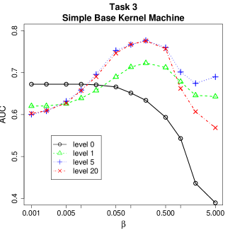
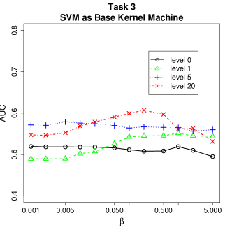
Figure 1: Average performance over 25 random splits of $V(\mathcal{G})$ into $V_{obs}(\mathcal{G})$ and $V_{miss}(\mathcal{G})$. Horizontal axis (logarithmic scale): tuning parameter $\beta$ for the initial diffusion kernel $\mathbf{K}_{\mathcal{G}}$; see equation (2). Vertical axis: performance measure, e.g., AP or AUC; see Section 4.3.

5 Discussion

To paraphrase our conclusions (C1) and (C2) above, we have essentially argued that we should put more emphasis on finding the “right” feature space rather than finding the “optimal” linear classifier (perhaps in the “wrong” feature space). One can use DKMs to do this. While the automatic and recursive kernel correction formula (10) is attractive, there clearly remains one important question that we haven’t quite addressed: how deep should we go?

Before we address this question, we first briefly mention interesting connections between our work and some recent literature on deep architectures in machine learning. The neural network was a leading algorithm for machine learning during the 1980’s, but it did not enjoy as wide a success as was initially anticipated. The main reason is because the back propagation algorithm is not practical for training neural networks that are more than a few layers deep. Recently, many arguments (e.g., Hinton and Salakhutdinov 2006; Sutskever and Hinton 2008; Bengio 2009) have been made that deep neural networks (i.e., neural networks with many layers) are necessary, and practically realistic algorithms have also emerged (e.g., Hinton et al. 2006; Larochelle et al. 2009). Our work provides further support for the idea of deep architectures.

By definition, the architecture of a deep neural network is necessarily complex. One has to make many decisions. How many layers? How many hidden components for each layer? In the landmark article (Hinton and Salakhutdinov 2006) on deep neural networks that appeared in the prestigious journal, Science, the authors showcased deep neural nets for a number of different tasks. A very striking feature of that article is that the authors used vastly different deep architectures for the different tasks, but there was little explanation on how those architectural decisions were made. We asked the first author of the Science article in person, after he delivered a seminar on the very subject. His answer was: one simply tries different architectures and picks the one that gives the best results. While this is not entirely satisfactory, we think such a limitation alone is no reason for anyone to deny that deep neural networks are a major advance in modern machine learning research. One cannot solve all problems at once. New ideas always lead to new problems, and that’s the very nature of scientific research.

At this moment, we don’t have an entirely satisfactory answer to the question of how deep a DKM one should use, except that we have empirically observed diminishing returns as we go to higher and higher levels, but this limitation alone in our work is no reason for us to reject the fact that DKMs can be quite useful.

Finally, it is not hard to see that the development of these DKMs (Section 3) does not rely on $\mathcal{G}$ being a graph. For example, if we abuse our notation and allow $\mathcal{G}$ to denote the usual $q$-dimensional Euclidean space, then we simply have a usual classification problem — $V_{obs}(\mathcal{G})$ simply becomes the set of training data and $V_{miss}(\mathcal{G})$, the set of unlabelled observations to be classified. Of course, in that case $\mathbf{K}_{\mathcal{G}}$ will no longer be the diffusion kernel, but, regardless of what it is, a level-0 kernel machine using $\mathbf{K}_{\mathcal{G}}$ will still be linear in its implicit feature space $\mathcal{F}$. Using the distance function $d_{\mathcal{F}}$, we can still do kernel density estimation in the space of $\mathcal{F}$, and obtain a level-1 kernel machine using a new kernel $\mathbf{K}_{\mathcal{F}}$. In other words, the idea of DKMs is general and not restricted to node classification on graphs. Whether they are actually useful for data structures other than graphs remains to be seen. We leave this to further investigation.

6 Summary

We have described the idea of using deep kernel machines for node classification on graphs. We have conducted a few experiments to show that linear classification in the implicit feature space of kernels commonly used for graph data (e.g., the diffusion kernel) is often not enough. When this is the case, one can apply the “kernel trick” again in the implicit feature space itself. Repeating this process leads to deep kernel machines (DKMs). Our experiments have shown that DKMs’ recursive, automatic kernel correction capability is especially useful when the initial kernel $\mathbf{K}_{\mathcal{G}}$ is not well specified. While the work we reported here is just a beginning and there remains much to be done, our results lend support to the idea of using deep architectures for machine learning that has recently emerged in the literature.

References

- Bengio (2009) Bengio, Y. (2009). Learning deep architectures for AI. Foundations and Trends in Machine Learning, 2(1), 1–127.
- Bishop (2006) Bishop, C. M. (2006). Pattern Recognition and Machine Learning. Springer-Verlag.
- Cristianini and Shawe-Taylor (2000) Cristianini, N. and Shawe-Taylor, J. (2000). An Introduction to Support Vector Machines and Other Kernel-based Learning Methods. Cambridge University Press.
- Hinton and Salakhutdinov (2006) Hinton, G. E. and Salakhutdinov, R. R. (2006). Reducing the dimensionality of data with neural networks. Science, 313, 504–507.
- Hinton et al. (2006) Hinton, G. E., Osindero, S., and Teh, Y. (2006). A fast learning algorithm for deep belief nets. Neural Computation, 18, 1527–1554.
- Kolaczyk (2009) Kolaczyk, E. D. (2009). Statistical Analysis of Network Data. Springer-Verlag.
- Lafferty and Lebanon (2005) Lafferty, J. and Lebanon, G. (2005). Diffusion kernels on statistical manifolds. Journal of Machine Learning Research, 6, 129–163.
- Larochelle et al. (2009) Larochelle, H., Bengio, Y., Louradour, J., and Lamblin, P. (2009). Exploring strategies for training deep neural networks. Journal of Machine Learning Research, 10, 1–40.
- Lazega (2001) Lazega, E. (2001). The Collegial Phenomenon: The Social Mechanisms of Cooperation Among Peers in a Corporate Law Partnership. Oxford University Press.
- Pepe (2003) Pepe, M. S. (2003). The Statistical Evaluation of Medical Tests for Classification and Prediction. Oxford University Press.
- Shawe-Taylor and Cristianini (2004) Shawe-Taylor, J. and Cristianini, N. (2004). Kernel Methods for Pattern Analysis. Cambridge University Press.
- Sutskever and Hinton (2008) Sutskever, I. and Hinton, G. E. (2008). Deep narrow sigmoid belief networks are universal approximators. Neural Computation, 20, 2629–2636.
- Vapnik (1995) Vapnik, V. N. (1995). The Nature of Statistical Learning Theory. Springer-Verlag.
- Zhu et al. (2006) Zhu, M., Su, W., and Chipman, H. A. (2006). LAGO: A computationally efficient approach for statistical detection. Technometrics, 48, 193–205.