Observables for FRW model with cosmological constant
in the framework of loop cosmology

Abstract

We consider a flat cosmological model with a free massless scalar field and the cosmological constant $\Lambda$ in the framework of loop quantum cosmology. The scalar field plays the role of an intrinsic time. We apply the reduced phase space approach. The dynamics of the model is solved analytically. We identify elementary observables and their algebra. The compound physical observables like the volume and the energy density of matter field are analysed. Both compound observables are bounded and oscillate in the $\Lambda<0$ case. The energy density is bounded and oscillates in the $\Lambda>0$ case. However, the volume is unbounded from above, but periodic. The difference between standard and nonstandard loop quantum cosmology is described.

I Introduction

The standard loop quantum cosmology (LQC) follows the Dirac quantization scheme. In this approach, one first defines the kinematical Hilbert space. Then, the physical states are determined by the requirement that the quantum constraint operator (in simple cases there may be only one constraint) vanishes on them. The space of solutions is used to construct the physical Hilbert space Ashtekar:2003hd ; Bojowald:2006da . There exists an alternative method, the reduced phase space approach, that we call nonstandard LQC. It consists in solving the dynamical constraint already at the classical level and the identification of physical observables. Examination of spectra of the corresponding quantum observables leads to description of the cosmological system. Such an approach has been recently applied to the quantization of a flat Friedmann-Robertson-Walker (FRW) model with a free massles scalar field Dzierzak:2009ip ; Malkiewicz:2009zd ; Malkiewicz:2009qv . In the present paper we consider an extension of the classical aspects of the model by including a contribution from the cosmological constant $\Lambda$.

Since the standard LQC seems to be very successful Ashtekar:2010qn , one may wonder what the motivation for developing the nonstandard LQC could be. Let us discuss it in more detail. The situation is that there are no precise observational data available to verify the predictions of quantum cosmology models. In such case a reasonable strategy seems to be comparing results obtained within alternative approaches. An agreement of results would prove that the procedure of quantization is correct. An agreement of such results with observational data (when they become available) would be the final goal. The above strategy underlies our paper. We wish to obtain results to be compared with the standard LQC results. On the other hand, an alternative method may improve our understanding of various conceptual issues like identification of Dirac’s observables, determination of the minimum length specifying critical energy density of matter field at the big bounce transition, quantum evolution of a system with Hamiltonian constraint, etc. Present paper addresses the first issue and begins the discussion of the second and third ones. They will be considered in our next paper presenting quantization of the present model.

II Hamiltonian

The gravitational part of the classical Hamiltonian, in the Ashtekar variables $(A^{i}_{a},E^{a}_{i})$, is the sum of the first class constraints

$$H_{g}=\frac{1}{16\pi G}\int_{\Sigma}d^{3}{\bf x}(N^{i}C_{i}+N^{a}C_{a}+NC),$$ (1)

where $\Sigma$ is the space-like part of spacetime $\mathbb{R}\times\Sigma$, and where

$$C_{i} = D_{a}E^{a}_{i}=\partial_{a}E^{a}_{i}+\epsilon_{ijk}A^{j}_{a}E^{a}_{k},$$ (2)

$$C_{a} = E^{b}_{i}F^{i}_{ab}-(1+\gamma^{2})K^{i}_{a}C_{i},$$ (3)

$$C = \frac{E^{a}_{i}E^{b}_{j}}{\sqrt{|\det E|}}\left(\epsilon^{ij}_{k}F^{k}_{ab}-2(1+\gamma^{2})K^{i}_{[a}K^{j}_{b]}\right)$$ (4)

($\gamma$ is the Barbero-Immirzi parameter). For the considered FRW model, the Gauss constraint $C_{i}$ as well as the spatial diffeomorphisms constraint $C_{a}$ are automatically fulfilled. The only nontrivial part is the scalar constraint $C$. Because for the homogeneous models $K^{i}_{a}=\frac{1}{\gamma}A^{i}_{a}$, the Hamiltonian simplifies to

$$H_{g}=-\frac{1}{\gamma^{2}}\frac{1}{16\pi G}\int_{\Sigma}d^{3}{\bf x}\frac{1}{\sqrt{|\det E|}}E^{a}_{i}E^{b}_{j}\epsilon^{ij}_{k}F^{k}_{ab}.$$ (5)

In LQC the gravitational degrees of freedom are parametrised by holonomies $h_{i}$ and fluxes $F_{i}$ (which are functionals of the Ashtekar variables). These are non-local functions used to construct a non-perturbative theory. The holonomies and fluxes are non-trivial $SU(2)$ variables satisfying the holonomy-flux algebra. However, in the highly symmetric spaces, like the FRW model considered here, the forms of these functions simplify.

In particular, in the flat FRW model the flux may be parametrised by $v$ variable and the holonomy is expressed in terms of $\beta$ variable Malkiewicz:2009qv . The variable $v$ is a physical volume defined as follows

$$v := \int_{\mathcal{V}}dx_{1}dx_{2}dx_{3}\sqrt{det\,q_{ab}}$$ (6)

$$= a^{3}\int_{\mathcal{V}}dx_{1}dx_{2}dx_{3}\sqrt{det\,q_{ab}^{0}}=:a^{3}\,V_{0},$$

where $\mathcal{V}\subset\Sigma$ is an elementary cell in the space with topology $\mathbb{R}^{3}$; $(x_{a})=(x^{a})=(x^{1},x^{2},x^{3})$ are Cartesian coordinates; $q_{ab}:=a^{2}\,q_{ab}^{0}$ is a physical 3-metric; $a$ is a scale factor; $q_{ab}^{0}dx^{a}dx^{b}:=dx_{1}^{2}+dx_{2}^{2}+dx_{3}^{2}$ defines a fiducial 3-metric; $V_{0}$ is a fiducial volume (it does not occur in final results). The $\beta$ variable, in the limit $\beta\rightarrow 0$, is linked to the Hubble factor $H=\dot{a}/a$ via the relation $\beta=\gamma H$.

In order to express the Hamiltonian, Eq. (5), in terms of holonomies and fluxes, the procedure of regularization has to be applied. The regularization introduces a new scale to the theory, namely the parameter $\lambda$. This can be understood as the length scale of the lattice discretization. The applied procedure of regularization and rewriting the Hamiltonian in terms of holonomies and fluxes is the same as known from the standard LQC. However, to the completeness of considerations we sum up the main step of this derivation in Appendix A. The obtained gravitational part of the Hamiltonian reads Ashtekar:2006wn

$$H^{(\lambda)}_{g}=-\frac{vN}{32\pi^{2}G^{2}\gamma^{3}\lambda^{3}}\sum_{ijk}\epsilon^{ijk}\text{tr}\left[h_{\Box_{ij}}h_{k}\left\{(h_{k})^{-1},v\right\}\right],$$

(7)

where $h_{\Box_{ij}}=h_{i}h_{j}(h_{i})^{-1}(h_{j})^{-1}$ is the holonomy around the square loop $\Box_{ij}$ (for more details see Dzierzak:2009ip ). $N$ is the lapse function. The elementary holonomy in the i-th direction reads

$$h_{i}=\cos\left(\frac{\lambda\beta}{2}\right)\mathbb{I}+2\sin\left(\frac{\lambda\beta}{2}\right)\tau_{i}$$ (8)

where $\tau_{i}=-\frac{i}{2}\sigma_{i}$ ($\sigma_{i}$ are the Pauli matrices). The holonomy (8) is calculated in the fundamental, $j=1/2$, representation of $SU(2)$. The factor $\lambda$ is the parameter of the theory that may be related with the minimum area of the loop. Namely, $\text{Ar}_{\Box_{ij}}=\lambda^{2}$ so $\lambda$ has the dimension of length. It is supposed to mark the scale when classical dynamics should be modified by quantum effects. It is expected that $\lambda\sim l_{\text{Pl}}$, but its precise value has to be fixed observationally. At present, one can only give the upper constraint on $\lambda$. Based on the observations of the cosmic microwave background radiation it was recently shown Mielczarek:2009zw that $\lambda\leq 7\cdot 10^{4}\,l_{\text{Pl}}$.

In the model considered in this paper, the total Hamiltonian is the sum of the gravity $H^{(\lambda)}_{g}$, cosmological constant $H_{\Lambda}$, and free scalar field $H_{\phi}$ parts

$$H^{(\lambda)}=:NC:=H^{(\lambda)}_{g}+H_{\Lambda}+H_{\phi},$$ (9)

where

$$H_{\Lambda}:=N\frac{v\Lambda}{8\pi G}~{}~{}~{}~{}\text{and}~{}~{}~{}~{}H_{\phi}:=N\frac{p^{2}_{\phi}}{2v}.$$ (10)

The insertion of the elementary holonomy (8) into Eq. (7) leads (for details, see Appendix A) to the expression

$$H^{(\lambda)}=N\left[-\frac{3}{8\pi G\gamma^{2}}\frac{\sin^{2}(\lambda\beta)}{\lambda^{2}}v+\frac{p^{2}_{\phi}}{2v}+v\frac{\Lambda}{8\pi G}\right]\approx 0.$$ (11)

The variables $(v,\beta,\phi,p_{\phi})$ parametrise the phase space, and the sign “$\,\approx\,$” reminds that the Hamiltonian is a constraint of the gravitational system under consideration.

The technical procedure leading to Eqs. (7) and (11) (presenting a Hamiltonian parametrized by $\lambda$) is identical in both standard and nonstandard LQC. The Hamiltonian must be the same, otherwise the comparison of both methods could not be done. The real difference arises when one begins the implementation of the Hamiltonian constraint, $H^{(\lambda)}\approx 0$. In the standard approach, one promotes Eq. (11) to an operator equation at the quantum level with the parameter $\lambda$ different from zero. Why is the parameter $\lambda$ kept different from zero? The technical answer is that in the limit $\lambda\rightarrow 0$ the regular constraint equation turns into the singular Wheeler-DeWitt equation Dzierzak:2008dy . The physical justification for keeping $\lambda\neq 0$ offered by the standard method is that in the loop representation used to quantize the kinematical level this representation does not exist for $\lambda=0$ Ashtekar:2003hd . In the second step of this method, one turns the classical constraint equation into an operator equation, which one defines consequently in the loop representation of the kinematical level Ashtekar:2006wn . This is why one keeps $\lambda\neq 0$ in the operator equation. Why one uses such an exotic representation which is not defined for $\lambda\neq 0?$ Further explanation is that such representation is an analog of the representation used at the kinematical level of loop quantum gravity (LQG) Ashtekar:2003hd . Is this answer satisfactory? It is commonly known that the LQG has not been constructed yet. The representation of the constraints algebra, based on the achievements of the kinematical level, has not been found yet. The problem is extremely difficult because the algebra is not a Lie, but a Poisson algebra (one structure function is not a constant but a function on phase space) TT . The users of the standard method believe that sooner or later this problem of LQG will be solved and LQC will be derived from LQG, so making use of an analogy to LQG is a healthy approach Ashtekar:2004eh . We think, it is an outstanding development, but far from being completed.

We are conscious that in the standard LQC the parameter $\lambda$ is fixed by taking into account the spectrum of the kinematical area operator of LQG (see, e.g. Ashtekar:2006wn ). Our approach, making strong reference to observational cosmology, may be treated as a sort of generalization of the standard approach. It is not an effective semi-classical version of the standard LQC, but a modified version of the classical cosmology model of general relativity. One can treat it as a one-parameter family of classical Hamiltonians, including the usual general relativity Hamiltonian as a special case for $\lambda=0$. It can be seen easily that the singularity becomes ‘resolved’ at the classical level, for $\lambda\neq 0$, due to the functional form of Eq. (11). It has been already discussed that the regularization, making use of approximating the curvature of connection by a holonomy around a loop with a finite length $\sim\lambda$ (see, appendix A) produces the big bounce Dzierzak:2009ip ; Malkiewicz:2009qv ; Haro:2009pt already at the classical level. Why should we quantize a cosmological model which is free from the cosmological singularity? There are at least three good reasons: (i) we must have a quantum model to make comparison with the standard method results which concern quantum level, (ii) classical energy density of matter depends on a free parameter $\lambda$ in such a way that it may become arbitrary big for small enough $\lambda$ (see Eqs. (44), (53) and (13)) so the system may enter a length scale where quantum effects have to be taken into account, and (iii) making predictions of our model for quantum cosmic data may be used to fix the free parameter $\lambda$, after such data become available.

The model with the Hamiltonian defined by Eq. (11) has been already studied Mielczarek:2008zv and analytical solutions have been found:

The Hamiltonian constraint, Eq. (11), can be rewritten as

$$\frac{2v^{2}}{p^{2}_{\phi}}=\frac{1}{\rho_{\text{c}}}\frac{1}{\left[\sin^{2}(\lambda\beta)-\delta\right]}\geq 0,$$ (12)

where $\rho_{\text{c}}$ is the critical energy density

$$\rho_{\text{c}}:=\frac{3}{8\pi G\gamma^{2}\lambda^{2}}$$ (13)

and $\delta$ is a parameter

$$\delta:=\frac{\rho_{\Lambda}}{\rho_{\text{c}}}=\frac{\Lambda}{3}\gamma^{2}\lambda^{2},$$ (14)

and where $\rho_{\Lambda}:=\frac{\Lambda}{8\pi G}$.

It turns out that for $\rho_{\Lambda}>\rho_{\text{c}}\ (\delta>1)$, the system has no physical solutions Mielczarek:2008zv . The physical solutions exist only for $\Lambda<\Lambda_{\text{c}}$, where

$$\Lambda_{\text{c}}:=8\pi G\rho_{\text{c}}=\frac{3}{\gamma^{2}\lambda^{2}},$$ (15)

which defines the critical value of the cosmological constant. This surprising result extends to the quantum level as well Bentivegna:2008bg ; Kaminski:2009pc .

In what follows we consider two cases: $\Lambda<0$ ($\delta<0$, anti-de Sitter) and $0<\Lambda<\Lambda_{\text{c}}$ ($0<\delta<1$, de Sitter).

III Equations of motion

The equations of motion for the system are defined by the Hamilton equation $\dot{f}=\left\{f,H^{(\lambda)}\right\}$, where the Poisson bracket is defined as follows

$$\{\cdot,\cdot\} := 4\pi G\gamma\left[\frac{\partial\cdot}{\partial\beta}\frac{\partial\cdot}{\partial v}-\frac{\partial\cdot}{\partial v}\frac{\partial\cdot}{\partial\beta}\right]$$ (16)

$$+ \frac{\partial\cdot}{\partial\phi}\frac{\partial\cdot}{\partial p_{\phi}}-\frac{\partial\cdot}{\partial p_{\phi}}\frac{\partial\cdot}{\partial\phi}.$$

The solutions of the Hamilton equation with $f\in(v,\beta,\phi,p_{\phi})$ define the kinematical phase space $\mathcal{F}_{\text{kin}}$. In turn, the solutions restricted by the Hamiltonian constraint, Eq. (11), define the physical phase space $\mathcal{F}_{\text{phys}}$.

For the function defined on $\mathcal{F}_{\text{phys}}$, the dynamics are governed by

$$\dot{f}=\left\{f,NC\right\}=\underbrace{\left\{f,N\right\}C}_{=\;0\ \text{on}\ \mathcal{F}_{\text{phys}}}+N\left\{f,C\right\}=N\left\{f,C\right\}.$$ (17)

Thus, the relational dynamics of variables $f$ and $g$ on $\mathcal{F}_{\text{phys}}$ is defined by

$$\frac{\dot{f}}{\dot{g}}=\frac{df}{dg}=\frac{\left\{f,C\right\}}{\left\{g,C\right\}}$$ (18)

so it is gauge independent. The specific choice of gauge can however simplify the calculations. In our considerations we choose the lapse function in the form

$$N=1/v.$$ (19)

The equations of motion read

$$\dot{v} = \{v,H^{(\lambda)}\}=\frac{3\sin(2\beta\lambda)}{2\gamma\lambda},$$ (20)

$$\dot{\beta} = \{\beta,H^{(\lambda)}\}=-\frac{4Gp^{2}_{\phi}\pi\gamma}{v^{3}},$$ (21)

$$\dot{\phi} = \{\phi,H^{(\lambda)}\}=\frac{p_{\phi}}{v^{2}},$$ (22)

$$\dot{p}_{\phi} = \{p_{\phi},H^{(\lambda)}\}=0.$$ (23)

An elementary observable $\mathcal{O}$ is a real function on the phase space that satisfies the equation (for a precise definition see Dzierzak:2009ip )

$$\{\mathcal{O},H^{(\lambda)}\}\approx 0.$$ (24)

It is clear that constants of motion of the Hamilton equations satisfy Eq. (24). We get immediately from Eq. (23) the first observable

$$\mathcal{O}_{1}=p_{\phi}.$$ (25)

Finding other observables needs definitely more effort.

Before we proceed to the task we would like to firstly make a comment on the relation between the classical cosmology and the model under considerations. In particular, we would like to show in which limit, the standard Friedmann equation is recovered.

We define the Hubble factor as follows $H:=\frac{1}{3v}\frac{dv}{dt}$, where $t$ is a coordinate time. We can insert Eq. (20) into this definition, however keeping in mind the fact that $\dot{v}=\frac{1}{N}\frac{dv}{dt}$, which results from Eq. (17). Taking square of the Hubble factor and inserting Eq. (12) we find

$$H^{2}=\frac{8\pi G}{3}\rho_{\phi}\left(1-\frac{\rho_{\phi}}{\rho_{\text{c}}}\right)+\frac{\Lambda}{3}\left(1-2\frac{\rho_{\phi}}{\rho_{\text{c}}}-\frac{\rho_{\Lambda}}{\rho_{\text{c}}}\right),$$ (26)

where we have defined $\rho_{\phi}:=\frac{p^{2}_{\phi}}{2v^{2}}$. Equation (26) is the modified Friedmann equation which results from the considered model. Let us consider the limit $\lambda\rightarrow 0$. Based on Eq. (13) we find $\lim_{\lambda\rightarrow 0}\rho_{\text{c}}=\infty$. Therefore in the limit of vanishing modification, $\lambda\rightarrow 0$, the classical Friedmann equation

$$H^{2}=\frac{8\pi G}{3}\rho_{\phi}+\frac{\Lambda}{3},$$ (27)

is recovered. Another issue is the correspondence with the standard cosmology. We see that the modifications become irrelevant when $\rho_{\phi}\ll\rho_{\text{c}}$ and $\rho_{\Lambda}\ll\rho_{\text{c}}$, and the form of Eq. (27) is recovered. Therefore, the correspondence takes place in the limit of low energy densities of matter and cosmological constant. However, while the matter energy density $\rho_{\phi}$ is diluted with the increase of volume $v$, the $\rho_{\Lambda}$ remains constant. Therefore the last term in Eq. (26), namely $-\frac{\Lambda}{3}\frac{\rho_{\Lambda}}{\rho_{\text{c}}}=-\frac{\Lambda}{3}\delta$, contributes also in the limit of the large volumes. As we will show later, the value of parameter $\delta$ is extremely low for the observationally determined value of cosmological constant. This additional constant term is therefore completely negligible and its present contribution cannot be verified observationally.

IV Anti-de Sitter (AdS)

Based on Eqs. (20) and (21) we find

$$\frac{d\beta}{dv}=-\frac{8\pi Gp^{2}_{\phi}\gamma^{2}\lambda}{3\sin(2\beta\lambda)v^{3}}.$$ (28)

Integrating the above equation we obtain the observable (as a constant of integration)

$$\mathcal{O}_{3}=\cos(2\beta\lambda)+\frac{8\pi G\gamma^{2}\lambda^{2}}{3v^{2}}\mathcal{O}_{1}^{2}.$$ (29)

Equations (21) and (22) give

$$\frac{d\beta}{d\phi}=-\frac{4\pi Gp_{\phi}\gamma}{v}.$$ (30)

Solving this equation gives the next observable

$$\mathcal{O}_{2} = \phi+\frac{2}{\sqrt{8\pi G}}\frac{\text{sgn}(p_{\phi})}{\sqrt{3(\mathcal{O}_{3}-1)}}\left[F\left(\beta\lambda\left|-\frac{2}{\mathcal{O}_{3}-1}\right.\right)\right.$$ (31)

$$- \left.F\left(\frac{\pi}{2}\left|-\frac{2}{\mathcal{O}_{3}-1}\right.\right)\right]$$

where $F$ is the Jacobi elliptic integral of the first kind

$$F(x|m)=\int_{0}^{x}\frac{d\theta}{\sqrt{1-m\sin^{2}(\theta)}}.$$ (32)

To get Eq. (31) we have spitted the integration of the righthand side of Eq. (32) as follows

$$\int_{\pi/2}^{x}\frac{d\theta}{\sqrt{1-m\sin^{2}\theta}} = \int_{0}^{x}\frac{d\theta}{\sqrt{1-m\sin^{2}\theta}}$$ (33)

$$- \int_{0}^{\pi/2}\frac{d\theta}{\sqrt{1-m\sin^{2}\theta}}.$$

The lower limit of the integration, in variable $\theta:=\lambda\beta$, is equal to $\pi/2$. With this particular choice, the limit $\Lambda\rightarrow 0$ leads to the expressions found in the case $\Lambda=0$. This limit will be discussed in more details in Sec. VI. In fact, the lower limit of integration can be set to be an arbitrary number. In particular, it can equals not $\pi/2$, but zero. This will not change the physics, but it will not lead to the expression for the observables found in the case $\Lambda\rightarrow 0$. It is so because the elementary observables are defined up to an additive constant.

One may verify that obtained observables satisfy the Lie algebra

$$\left\{\mathcal{O}_{1},\mathcal{O}_{3}\right\} = 0,$$ (34)

$$\left\{\mathcal{O}_{2},\mathcal{O}_{3}\right\} = 0,$$ (35)

$$\left\{\mathcal{O}_{2},\mathcal{O}_{1}\right\} = 1.$$ (36)

This algebra can be simplified since the observable $\mathcal{O}_{3}$ can be eliminated due to the Hamiltonian constraint which reads

$$\mathcal{O}_{3}=1-2\delta.$$ (37)

Making use of Eq. (37) we may rewrite $\mathcal{O}_{2}$ in the form

$$\mathcal{O}_{2}=\phi+\frac{\text{sgn}(p_{\phi})}{\sqrt{12\pi G(-\delta)}}\left[F\left(\beta\lambda\left|\frac{1}{\delta}\right.\right)-K\left(\frac{1}{\delta}\right)\right]$$ (38)

where $K\left(m\right)=F\left(\pi/2\left|m\right.\right)$. It Appendix B, the form of the Poisson bracket on $\mathcal{F}_{\text{phys}}$ has been derived. The observables $\mathcal{O}_{1}$ and $\mathcal{O}_{2}$ satisfy on $\mathcal{F}_{\text{phys}}$ the Lie algebra

$$\left\{\mathcal{O}_{2},\mathcal{O}_{1}\right\}=1,$$ (39)

where

$$\left\{\cdot,\cdot\right\}:=\frac{\partial\cdot}{\partial\mathcal{O}_{2}}\frac{\partial\cdot}{\partial\mathcal{O}_{1}}-\frac{\partial\cdot}{\partial\mathcal{O}_{1}}\frac{\partial\cdot}{\partial\mathcal{O}_{2}}.$$ (40)

Equation (38) can be inverted to the form

$$\lambda\beta=\text{am}\left(\sqrt{12\pi G(-\delta)}\text{sgn}(p_{\phi})(\mathcal{O}_{2}-\phi)+K\left(\frac{1}{\delta}\right)\left|\frac{1}{\delta}\right.\right),$$ (41)

where am$(x|m)=F^{-1}(x|m)$ in an amplitude of the Jacobi integral.

The energy density is found to be

$$\rho=\rho_{\phi}+\rho_{\Lambda}=\frac{p^{2}_{\phi}}{2v^{2}}+\frac{\Lambda}{8\pi G}.$$ (42)

Due to the Hamiltonian constraint it reads

$$\rho=\rho_{\text{c}}\,\sin^{2}(\lambda\beta).$$ (43)

Using Eq. (41) we may rewrite Eq. (43) in the form

$$\rho(\phi)=\rho_{\text{c}}\text{sn}^{2}\left(\sqrt{12\pi G(-\delta)}(\mathcal{O}_{2}-\phi)+K\left(\frac{1}{\delta}\right)\left|\frac{1}{\delta}\right.\right),$$ (44)

where $\text{sn}(\cdot|\cdot):=\sin(\text{am}(\cdot|\cdot))$. We plot this dependence in Fig. 1.

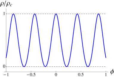
Figure 1: Plot of $\rho(\phi)$ for $\delta=-1$ and $\mathcal{O}_{2}=0$. Here, the period of oscillations is equal to $\Delta\phi\simeq 0.427$

Based on Eqs. (12) and (41) we derive an expression for the volume observable in terms of elementary observables and an evolution parameter $\phi$

$$v(\phi)=\frac{|\mathcal{O}_{1}|}{\sqrt{2\rho_{c}}}\frac{1}{\sqrt{\text{sn}^{2}\left(\sqrt{12\pi G(-\delta)}(\mathcal{O}_{2}-\phi)+K\left(\frac{1}{\delta}\right)\left|\frac{1}{\delta}\right.\right)-\delta}}.$$ (45)

The plot of this function is shown in Fig. 2.

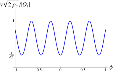
Figure 2: Plot of $v(\phi)$ for $\delta=-1$ and $\mathcal{O}_{2}=0$. Here, the period of oscillations is equal to $\Delta\phi\simeq 0.427$

The solution for the volume $v$ are non-singular oscillations with the maximal and minimal values given by

$$v_{\text{max}} = \frac{|\mathcal{O}_{1}|}{\sqrt{2\rho_{c}}}\frac{1}{\sqrt{-\delta}}\ \ \mapsto\ \ \rho=0,$$ (46)

$$v_{\text{min}} = \frac{|\mathcal{O}_{1}|}{\sqrt{2\rho_{c}}}\frac{1}{\sqrt{1-\delta}}\ \ \mapsto\ \ \rho=\rho_{\text{c}}.$$ (47)

Equation (46) tells that when the volume is maximal, the total energy density equals zero. However, the matter density does not vanish, since due to Eq. (44) we have $\rho_{\phi}=-\rho_{\Lambda}=-\frac{\Lambda}{8\pi G}>0$ (as $\Lambda<0$ in AdS case).

The period of oscillations can be written as

$$\Delta\phi=\frac{2K\left(\frac{1}{\delta}\right)}{\sqrt{12\pi G(-\delta)}}.$$ (48)

V de Sitter (dS)

In this case the considerations are similar to those presented in the previous section. However, finding a suitable definition of the observable $\mathcal{O}_{2}$ requires some additional analysis. Namely, in this case

$$\sin^{2}(\lambda\beta)\geq\delta$$ (49)

that result from Eq. (12). Thus, $\lambda\beta\in[\theta_{0}+n\pi,(1-n)\pi-\theta_{0}]$, where $n\in\mathbb{Z}$ and $\theta_{0}:=\arcsin(\sqrt{\delta})$. The equation for the observable $\mathcal{O}_{2}$ takes the form

$$d\mathcal{O}_{2}=d\phi+\frac{\text{sgn}(p_{\phi})}{\sqrt{12\pi G}}\frac{\lambda d\beta}{\sqrt{\sin^{2}(\lambda\beta)-\delta}}.$$ (50)

The integration of this equation can be done by using the Jacobi function (see Eq. (32)) as in anti-de Sitter case. The lower limit of integration is set to be $\pi/2$ and the relation (33) is applied. The choice of the lower limit is dictated by the limit $\Lambda\rightarrow 0$. For the $\theta<\theta_{0}$ the integration gives an imaginary number. However, due to relation (33) these contributions cancel out. Finally, we get

$$\mathcal{O}_{2}=\phi+\frac{\text{sgn}(p_{\phi})}{\sqrt{12\pi G\delta}}\frac{1}{i}\left[F\left(\beta\lambda\left|\frac{1}{\delta}\right.\right)-K\left(\frac{1}{\delta}\right)\right],$$ (51)

which is a real function on $\mathcal{F}_{\text{phys}}$ for $\lambda\beta\in[\theta_{0},\pi-\theta_{0}]$. The algebra of observables is the same as in the anti-de Sitter case.

Equation (51) can be inverted to the form

$$\sin^{2}(\lambda\beta)=\delta\text{dn}^{2}\left(\sqrt{12\pi G\delta}(\mathcal{O}_{2}-\phi)+K\left|1-\frac{1}{\delta}\right.\right)$$ (52)

where we defined $K:=K\left(1-\frac{1}{\delta}\right)$, so we have

$$\rho(\phi)=\rho_{\text{c}}\delta\text{dn}^{2}\left(\sqrt{12\pi G\delta}(\mathcal{O}_{2}-\phi)+K\left|1-\frac{1}{\delta}\right.\right).$$ (53)

The function $\text{dn}(\cdot|\cdot)$ is defined as $\text{dn}(u|m):=\sqrt{1-m\sin^{2}[\text{am}(u|m)]}$. We plot function (53) in Fig. 3.

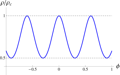
Figure 3: Plot of $\rho(\phi)$ for $\delta=0.5$ and $\mathcal{O}_{2}=0$. Here, $\Delta\phi\simeq 0.604$.

Making use of Eqs. (52) and (12) we find

$$v(\phi)=\frac{|\mathcal{O}_{1}|}{\sqrt{2\rho_{c}(1-\delta)}}\frac{1}{\left|\text{sn}\left(\sqrt{12\pi G\delta}(\mathcal{O}_{2}-\phi)+K\left|1-\frac{1}{\delta}\right.\right)\right|}.$$ (54)

We present this function in Fig. 4.

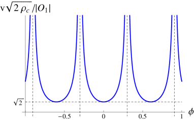
Figure 4: Plot of $v(\phi)$ for $\delta=0.5$ and $\mathcal{O}_{2}=0$. Here, $\Delta\phi\simeq 0.604$.

The solution is periodic

$$v(\phi)=v(\phi+n\,\Delta\phi),$$ (55)

where $n\in\mathbb{Z}$ and

$$\Delta\phi:=\frac{2K\left(1-\frac{1}{\delta}\right)}{\sqrt{12\pi G\delta}}.$$ (56)

However, contrary to the Anti-de Sitter case, the periodicity does not mean that the volume oscillates. The cycles are separated by asymptotes with $v\rightarrow\infty$. Each cycle is called a bounce. The bounces are disconnected and define quite independent solutions. Within a bounce, the value of the scalar field change by $\Delta\phi$. One can find that this corresponds to the evolution of the system from $t=-\infty\,$ to $\,t=+\infty$, where $t$ in the coordinate time. Thus, each period corresponds to the same dS universe.

It turns out Kaminski:2009pc ; WK that in the standard LQC the quantum evolution of semi-classical states interpolate between the trajectories in the adjacent eras shown in Fig. 4, forming a cyclic system. We plan to examine this interesting issue, within the nonstandard LQC, in our next paper concerning a quantum version of the model.

The maximum and minimum of of the volume, and the corresponding energy densities are

$$v_{\text{max}} = \infty\ \ \mapsto\ \ \rho=\rho_{\Lambda},$$ (57)

$$v_{\text{min}} = \frac{|\mathcal{O}_{1}|}{\sqrt{2\rho_{c}}}\frac{1}{\sqrt{1-\delta}}\ \ \mapsto\ \ \rho=\rho_{\text{c}}.$$ (58)

It may appear to be strange that as the maximum volume equals infinity, the total energy density does not vanish. However, this counter-intuitive result is correct since due to Eq. (44) the matter term goes to zero as the volume approaches infinity, whereas the $\Lambda$-term stays finite and equals $\Lambda/8\pi G>0$ (as $\Lambda>0$ in dS case).

VI The limit $\delta\rightarrow 0$

In the case $\delta=0$, the observables take the following form

$$\mathcal{O}_{1} = p_{\phi},$$ (59)

$$\mathcal{O}_{2} = \phi+\frac{\text{sgn}(p_{\phi})}{\sqrt{12\pi G}}\ln\left|\tan\left(\frac{\beta\lambda}{2}\right)\right|.\$$ (60)

To find the observable Eq. (60), we have integrated Eq. (30) taking into account the Hamiltonian constraint with $\delta=0$.

These observables satisfy the same Lie algebra as in the case $\delta\neq 0$. Namely, $\left\{\mathcal{O}_{2},\mathcal{O}_{1}\right\}=1$. Making use of the identity

$$\ln\left|\tan\left(\frac{\beta\lambda}{2}\right)\right|=-\text{arth}\left[\cos(\beta\lambda)\right],$$ (61)

one can find that the observables, Eqs. (59) and (60), are the same as those derived in Dzierzak:2009ip .

The elementary observables play the role of ‘building blocs’ used to define composite observables. In particular, one can find an expression for the volume

$$v=\frac{|\mathcal{O}_{1}|}{\sqrt{2\rho_{\text{c}}}}\cosh\left[\sqrt{12\pi G}(\mathcal{O}_{2}-\phi)\right],$$ (62)

as well as for the energy density

$$\rho=\frac{\rho_{\text{c}}}{\cosh^{2}\left[\sqrt{12\pi G}(\mathcal{O}_{2}-\phi)\right]}.$$ (63)

These compound observables are gauge independent and overlap with those found in Dzierzak:2009ip .

Now, let us discuss the limit $\delta\rightarrow 0$, for fixed $\lambda$. The observable $\mathcal{O}_{1}$ remains unchanged as it is independent on $\delta$. Let us examine the case of the observable $\mathcal{O}_{2}$. Here the situation for both anti-de Sitter and se Sitter case looks the same. Equations (38) and (51) can be written as

$$\mathcal{O}_{2}=\phi+\frac{\text{sgn}(p_{\phi})}{\sqrt{12\pi G}}\int_{\pi/2}^{\lambda\beta}\frac{d\theta}{\sqrt{\sin^{2}\theta-\delta}}.$$ (64)

We have

$$\lim_{\delta\rightarrow 0^{\pm}}\int_{\pi/2}^{x}\frac{d\theta}{\sqrt{\sin^{2}\theta-\delta}}=\int_{\pi/2}^{x}\frac{d\theta}{\sin\theta}=\ln\left|\tan\left(\frac{x}{2}\right)\right|$$ (65)

in the definition of $\mathcal{O}_{2}$. Thus, in both limits $\delta\rightarrow 0^{\pm}$ the expression Eq. (60) is recovered.

Now, let us try to get Eqs. (62) and (63) by taking the limit $\delta\rightarrow 0^{\pm}$. Firstly, let us consider de Sitter’s case. We rewrite equations (53) and (54) in the form

$$\rho = \rho_{\text{c}}\left[\delta-(\delta-1)\sin^{2}\varphi\right],$$ (66)

$$v = \frac{|\mathcal{O}_{1}|}{\sqrt{2\rho_{\text{c}}(1-\delta)}}\frac{1}{|\sin\varphi|},$$ (67)

where

$$\varphi=\text{am}\left[\sqrt{12\pi G\delta}(\mathcal{O}_{2}-\phi)+K\left|1-\frac{1}{\delta}\right.\right].$$ (68)

The last equality can be written as

$$\sqrt{12\pi G}(\mathcal{O}_{2}-\phi)=\int_{\pi/2}^{\varphi}\frac{d\theta}{\sqrt{\delta-(\delta-1)\sin^{2}\theta}}.$$ (69)

Taking the limit $\delta\rightarrow 0^{+}$, we get

$$\sqrt{12\pi G}(\mathcal{O}_{2}-\phi)=\int_{\pi/2}^{\varphi}\frac{d\theta}{\sin\theta}=\ln\left|\tan\left(\frac{\varphi}{2}\right)\right|$$ (70)

which can be rewritten as

$$\sin^{2}{\varphi}=\frac{1}{\cosh^{2}\left[\sqrt{12\pi G}(\mathcal{O}_{2}-\phi)\right]}.$$ (71)

It is clear now, that in the limit $\delta\rightarrow 0^{+}$, Eq. (66) and Eq. (67) turn into Eq. (63) and Eq. (62), respectively.

In the anti-de Sitter case the procedure is similar. This way both limits, $\delta\rightarrow 0^{\pm}$, lead to the same expressions for the density and the volume.

Now, let us determine the parameter $\delta$ from observations. The cosmological constant $\Lambda$ can be related with the observed dark energy, which dominates the energy density of the Universe. In this case one can rewrite the definition Eq. (14) in the form

$$\delta=\frac{1}{c^{2}}\Omega_{\Lambda}H^{2}_{0}\gamma^{2}\lambda^{2},$$ (72)

where $\Omega_{\Lambda}$ is the fractional density of the cosmological constant, $H_{0}$ is the present value of the Hubble parameter, and $c$ is the speed of light. The five years observations of the WMAP satellite yield $\Omega_{\Lambda}=0.742\pm 0.030$ and $H_{0}=71.9^{+2.6}_{-2.7}\ \text{km}\ \text{s}^{-1}\ \text{Mpc}^{-1}$ Dunkley:2008ie . Assuming that $\lambda=l_{\text{Pl}}$, where $\l_{\text{Pl}}$ is the Planck length and $\gamma=\gamma_{M}=0.2375\,$ Meissner:2004ju , we find

$$\delta=6.6\cdot 10^{-124}$$ (73)

which is an extremely small value. Such a small vale of $\delta$ is connected with the known discrepancy between observed value of the cosmological constant and the energy density of the quantum vacuum. Since $\delta>0$, the present observations favour dS case rather than AdS. It is, however, not excluded that the AdS phase had some realization in the past.

VII Conclusion

The density and the volume are functions of the elementary observables and an evolution parameter $\phi$. They become observables for each fixed value of this parameter as in such a case they satisfy Eq. (24). Due to Eq. (22) the parameter changes monotonically so it suits the purpose.

For any value of the cosmological constant $\Lambda$, considered in our paper, the elementary observables satisfy the same simple Lie algebra $\left\{\mathcal{O}_{2},\mathcal{O}_{1}\right\}=1$, on the constraint surface. The elementary observables serve as building blocks for composite ones. They correspond to the constants of motion specifying dynamics so they have physical meaning, but they are not required to be measurable.

The composite observables are defined on the physical phase space and have clear physical interpretation, so they are expected to be detectable in observational cosmology. The volume is bounded and oscillates in the AdS case. It is bounded from below and diverges in the dS case, as expected. The energy density is bounded in both cases. We have shown that in the limit $\Lambda\rightarrow 0^{\pm}$ the observables obtained for the case $\Lambda=0$ are recovered. Thus, our results are consistent.

The initial big-bang singularity turns into the big-bounce transition. The density is a function of a free parameter $\lambda$ and blows up as $\lambda\rightarrow 0$, which corresponds to the case when there is no modification of the Hamiltonian by the holonomies. In both standard and nonstandard LQC $\lambda$ is a free parameter. It seems there is no satisfactory way to determine its theoreticall value, but forthcoming observtional data may bring some resolution to this problem. We have already addressed this issue in the context of the standard LQC Dzierzak:2008dy and in the nonstandard LQC Dzierzak:2009ip ; Malkiewicz:2009qv . Some preliminary agreement with our results (without reference to ours) may be found in Sec. VI of an updated version 4 of Ashtekar:2007em . One discusses there ‘parachuting by hand’ of the results from full LQG into LQC, since the derivation of LQC from LQG has not been obtained yet.

One usually relates the violation of the Lorentz symmetry with quantum gravity effects. Recent observations suggest nature that the scale of the Lorentz symmetry violation is greater than $1.2E_{\text{Pl}}=1.5\cdot 10^{19}\text{GeV}$, which corresponds to the length scale $0.8l_{\text{Pl}}$. If quantum effects lead to the violation of the Lorentz symmetry, then the length scale of this effect should be related with $\lambda$. In such a case the astrophysical observations of the $\gamma-$ray bursts, like those presented in nature , can be potentially used to constrain the parameter $\lambda$. However, an explicit functional form of this relation is unknown. On the other hand, the observations like nature are still ambiguous due to low statistics. Thus, one cannot impose on $\lambda$ any realistic astrophysical constraints yet.

Our method relies on a direct link with observational data due to the unknown value of $\lambda$. This may make our model suitable for describing observational data despite the fact that FRW may have too much symmetry to be a realistic model of the Universe. Taking theoretically determined $\lambda$ from incomplete LQG, in the standard LQC, seems to give a model of the Universe less realistic than ours. We believe that lacking of theoretically determined numerical value of $\lambda$ is rather meritorious than problematic.

In our next paper we shall present quntization of the model considered here. This will enable us making complete comparison of the standard and the nonstandard LQC.

Appendix A Modified Hamiltonian

In this appendix we give more details on the modified gravitational Hamiltonian used it this paper. In particular, we derive the form of the regularized Hamiltonian, Eq. (7). Later, we show how this Hamiltonian simplifies to Eq. (11) after the expression for the holonomy $h_{i}$ in applied. We begin from Eq. (5). Applying the classical identity

$$\frac{1}{\sqrt{|\det E|}}E^{a}_{i}E^{b}_{j}\epsilon^{ij}_{k}F^{k}_{ab}=\frac{1}{4\pi G\gamma}\epsilon^{abc}\{A^{i}_{c},v\}F_{abi},$$ (74)

and the trace of a product of the $SU(2)$ variables we find

$$H_{g}=\frac{1}{32\pi^{2}G^{2}}\frac{1}{\gamma^{3}}\int_{\Sigma}d^{3}{\bf x}N\epsilon^{abc}\text{tr}\left[F_{ab}\{A_{c},v\}\right].$$ (75)

Regularization of this Hamiltonian can be performed with use of expressions

$${{}^{o}}e^{a}_{k}\{A_{a},v\}\approx-\frac{1}{\mu V^{1/3}_{0}}h_{k}\{h^{-1}_{k},v\}$$ (76)

and

$$h_{\Box_{ij}} = h_{i}h_{j}(h_{i})^{-1}(h_{j})^{-1}$$ (77)

$$\approx \mathbf{I}+\mu^{2}V_{0}^{2/3}F_{ab}{{}^{o}}e^{a}_{i}{{}^{o}}e^{b}_{j},$$

where the fiducial triad ${{}^{o}}e^{a}_{i}$ dual to the fiducial cotriad ${{}^{o}}\omega_{a}^{i}$ defined as $q_{ab}{{}^{o}}=\delta_{ij}{{}^{o}}\omega_{a}^{i}{{}^{o}}\omega_{b}^{i}$. Here $\mu V^{1/3}_{0}$ is the coordinate length of the path along which the elementary holonomy $h_{i}$ is calculated. The $\mu$ is a dimensionless parameter which controls the length. In the limit $\mu\rightarrow 0$, Eqs. (76) and (77) become equalities. Combining Eq. (76) and Eq. (77) one can write

$$\epsilon^{ijk}\text{tr}\left[h_{\Box_{ij}}h_{k}\{h^{-1}_{k},v\}\right]=$$

$$-\mu^{3}V_{0}\epsilon^{ijk}{{}^{o}}e^{a}_{i}{{}^{o}}e^{b}_{j}{{}^{o}}e^{c}_{k}\text{tr}\left[F_{ab}\{A_{c},v\}\right].$$ (78)

Based on this relation with $\epsilon^{ijk}{{}^{o}}e^{a}_{i}{{}^{o}}e^{b}_{j}{{}^{o}}e^{c}_{k}=\epsilon^{abc}$ and restricting the spatial integration to the fiducial volume $V_{0}$, one can regularize Eq. (75) into the form

$$H_{g}^{(\lambda)}=-\frac{vN}{32\pi^{2}G^{2}\gamma^{3}\lambda^{3}}\sum_{ijk}\epsilon^{ijk}\text{tr}\left[h_{\Box_{ij}}h_{k}\{h^{-1}_{k},v\}\right],$$

(79)

where $\lambda^{3}=\mu^{3}v=$ const. This condition means that the physical size of the link $\lambda$ remains constant during the evolution. The choice is motivated by the correspondence with the classical cosmology for the large values of volume $v$ and is equivalent to the so-called improved scheme of LQC Ashtekar:2006wn . The classical unmodified Hamiltonian of the FRW model can be recovered from $\lim_{\lambda\rightarrow 0}H_{g}^{(\lambda)}=H_{g}$.

Inserting the elementary holonomy

$$h_{k}=\cos\left(\frac{\lambda\beta}{2}\right)\mathbb{I}+2\sin\left(\frac{\lambda\beta}{2}\right)\tau_{k}$$ (80)

and its inversion

$$(h_{k})^{-1}=\cos\left(\frac{\lambda\beta}{2}\right)\mathbb{I}-2\sin\left(\frac{\lambda\beta}{2}\right)\tau_{k}$$ (81)

into the Hamiltonian [Eq. (79)]. Next, we find that

$$h_{k}\left\{(h_{k})^{-1},v\right\}=h_{k}4\pi G\frac{\partial}{\partial\beta}(h_{k})^{-1}=-4\pi G\gamma\lambda\tau_{k}.$$ (82)

To get this relation we have used the definition of the Poisson bracket, Eq. (16), and the equality $\tau_{k}^{2}=-\frac{1}{4}\mathbb{I}$. Then, making use of Eq. (82) turns the Hamiltonian, Eq. (79), into

$$H^{(\lambda)}_{g}=\frac{vN}{8\pi G\gamma^{2}\lambda^{2}}\sum_{ijk}\epsilon^{ijk}\text{tr}\left[h_{\Box_{ij}}\tau_{k}\right].$$ (83)

At this stage, the relation

$$\text{tr}\left[h_{\Box_{ij}}\tau_{k}\right]=-\frac{\epsilon_{ijk}}{2}\sin^{2}(\lambda\beta)$$ (84)

can be applied. To derive Eq. (84), we insert Eq. (80) and Eq. (81) into the definition of $h_{\Box_{ij}}$, and use the formulae

$$\text{tr}[\mathbb{I}] = 2,$$ (85)

$$\text{tr}[\tau_{i}] = 0,$$ (86)

$$\text{tr}[\tau_{i}\tau_{j}] = -\frac{1}{2}\delta_{ij},$$ (87)

$$\text{tr}[\tau_{i}\tau_{j}\tau_{k}] = -\frac{1}{4}\epsilon_{ijk},$$ (88)

as well as $[\tau_{i},\tau_{j}]=\epsilon_{ijk}\tau_{k}$. Afterwards, we use Eq. (84) to get

$$\sum_{ijk}\epsilon^{ijk}\text{tr}\left[h_{\Box_{ij}}\tau_{k}\right] = -\frac{1}{2}\sin^{2}(\lambda\beta)\sum_{ijk}\epsilon^{ijk}\epsilon_{ijk}$$ (89)

$$= -3\sin^{2}(\lambda\beta).$$

Finally, inserting Eq. (89) into Eq. (83) gives

$$H^{(\lambda)}_{g}=-\frac{3N}{8\pi G\gamma^{2}}\frac{\sin^{2}(\lambda\beta)}{\lambda^{2}}\,v.$$ (90)

The standard Friedmann equation can be obtained from Eq. (90) in the limit $\beta\rightarrow 0$ (limit of small Hubble factor) if we complete it by the matter Hamiltonian.

Appendix B Symplectic form

The symplectic form corresponding to the Poisson bracket, Eq. (16), reads

$$\omega=\frac{1}{4\pi G\gamma}d\beta\wedge dv+d\phi\wedge dp_{\phi}.$$ (91)

Let us find the symplectic form $\Omega$ on the surface of constraints, namely

$$\Omega:=\left.\omega\right|_{H^{(\lambda)}=0}.$$ (92)

Differentiating the Hamiltonian constraint we find

$$-\frac{6}{8\pi G\gamma^{2}\lambda}\sin(\lambda\beta)\cos(\lambda\beta)d\beta+\frac{p_{\phi}dp_{\phi}}{v^{2}}-\frac{p^{2}_{\phi}}{v^{3}}dv=0.$$ (93)

Based on this expression we obtain

$$\omega=\left(\frac{1}{4\pi G\gamma}\frac{v}{p_{\phi}}d\beta+d\phi\right)\wedge dp_{\phi}.$$ (94)

Differentiating $\mathcal{O}_{2}$ we find

$$d\mathcal{O}_{2}=d\phi+\frac{\text{sgn}(p_{\phi})}{\sqrt{12\pi G}}\frac{\lambda d\beta}{\sqrt{\sin^{2}(\lambda\beta)-\delta}}.$$ (95)

This expression, due to the Hamiltonian constraint, reads

$$d\mathcal{O}_{2}=d\phi+\frac{1}{4\pi G\gamma}\frac{v}{p_{\phi}}d\beta.$$ (96)

Inserting Eq. (96) to Eq. (94) we finally get

$$\Omega=d\mathcal{O}_{2}\wedge d\mathcal{O}_{1}.$$ (97)

Thus, the Poisson bracket on $\mathcal{F}_{\text{phys}}$ takes the form

$$\left\{\cdot,\cdot\right\}:=\frac{\partial\cdot}{\partial\mathcal{O}_{2}}\frac{\partial\cdot}{\partial\mathcal{O}_{1}}-\frac{\partial\cdot}{\partial\mathcal{O}_{1}}\frac{\partial\cdot}{\partial\mathcal{O}_{2}}.$$ (98)

References

- (1) A. Ashtekar, M. Bojowald and J. Lewandowski, “Mathematical structure of loop quantum cosmology”, Adv. Theor. Math. Phys. 7, 233 (2003) [arXiv:gr-qc/0304074].
- (2) M. Bojowald, “Loop quantum cosmology”, Living Rev. Rel. 8, 11 (2005) [arXiv:gr-qc/0601085].
- (3) P. Dzierzak, P. Malkiewicz and W. Piechocki, “Turning big bang into big bounce. I. Classical dynamics,” Phys. Rev. D 80, 104001 (2009) [arXiv:0907.3436].
- (4) P. Malkiewicz and W. Piechocki, “Energy Scale of the Big Bounce,” Phys. Rev. D 80, 063506 (2009) [arXiv:0903.4352].
- (5) P. Malkiewicz and W. Piechocki, “Turning big bang into big bounce: II. Quantum dynamics,” arXiv:0908.4029.
- (6) A. Ashtekar, “The Big Bang and the Quantum,” arXiv:1005.5491 [gr-qc].
- (7) A. Ashtekar, T. Pawlowski and P. Singh, “Quantum nature of the big bang: Improved dynamics,” Phys. Rev. D 74, 084003 (2006) [arXiv:gr-qc/0607039].
- (8) P. Dzierzak, J. Jezierski, P. Malkiewicz and W. Piechocki, “The minimum length problem of loop quantum cosmology,” Acta Phys. Polon. B 41 (2010) 717 [arXiv:0810.3172 [gr-qc]].
- (9) T. Thiemann Modern Canonical Quantum General Relativity (Cambridge: Cambridge University Press, 2007).
- (10) A. Ashtekar and J. Lewandowski, “Background independent quantum gravity: A status report”, Class. Quant. Grav. 21, R53 (2004). [arXiv:gr-qc/0404018].
- (11) J. Haro and E. Elizalde, “Effective gravity formulation that avoids singularities in quantum FRW cosmologies,” arXiv:0901.2861 [gr-qc].
- (12) J. Mielczarek, “Possible observational effects of loop quantum cosmology,” Phys. Rev. D 81, 063503 (2010), [arXiv:0908.4329].
- (13) J. Mielczarek, T. Stachowiak and M. Szydlowski, “Exact solutions for Big Bounce in loop quantum cosmology,” Phys. Rev. D 77, 123506 (2008) [arXiv:0801.0502].
- (14) E. Bentivegna and T. Pawlowski, “Anti-deSitter universe dynamics in LQC,” Phys. Rev. D 77, 124025 (2008) [arXiv:0803.4446].
- (15) W. Kaminski and T. Pawlowski, “The LQC evolution operator of FRW universe with positive cosmological constant,” Phys. Rev. D 81 (2010) 024014 [arXiv:0912.0162 [gr-qc]].
- (16) A. A. Abdo et al., “A limit on the variation of the speed of light arising from quantum gravity effects”, Nature 462, 331 (2009).
- (17) J. Dunkley et al. [WMAP Collaboration], “Five-Year Wilkinson Microwave Anisotropy Probe (WMAP) Observations: Likelihoods and Parameters from the WMAP data,” Astrophys. J. Suppl. 180 (2009) 306 [arXiv:0803.0586 [astro-ph]].
- (18) W. Kaminski, private communication.
- (19) K. A. Meissner, “Black hole entropy in loop quantum gravity,” Class. Quant. Grav. 21 (2004) 5245 [arXiv:gr-qc/0407052].
- (20) A. Ashtekar, A. Corichi and P. Singh, “Robustness of key features of loop quantum cosmology,” arXiv:0710.3565, v4 [Phys. Rev. D 77, 024046 (2008) ].