Josephson effect through a multilevel dot near a singlet-triplet transition

Abstract

We investigate the Josephson effect through a two-level quantum dot with an exchange coupling between two dot electrons. We compute the superconducting phase relationship and construct the phase diagram in the superconducting gap–exchange coupling plane in the regime of the singlet-triplet transition driven by the exchange coupling. In our study two configurations for the dot-lead coupling are considered: one where effectively only one channel couples to the dot, and the other where the two dot orbitals have opposite parities. Perturbative analysis in the weak-coupling limit reveals that the system experiences transitions from 0 to $\pi$ (negative critical current) behavior, depending on the parity of the orbitals and the spin correlation between dot electrons. The strong coupling regime is tackled with the numerical renormalization group method, which first characterizes the Kondo correlations due to the dot-lead coupling and the exchange coupling in the absence of superconductivity. In the presence of superconductivity, many-body correlations such as two-stage Kondo effect compete with the superconductivity and the comparison between the gap and the relevant Kondo temperature scales allows to predict a rich variety of phase diagrams for the ground state of the system and for the Josephson current. Numerical calculations predicts that our system can exhibit Kondo-driven 0-$\pi$-0 or $\pi$-0-$\pi$ double transitions and, more interestingly, that if proper conditions are met a Kondo-assisted $\pi$-junction can arise, which is contrary to a common belief that the Kondo effect opens a resonant level and makes the 0-junction. Our predictions could be probed experimentally for a buckminster fullerene sandwiched between two superconductors.

I Introduction

The Josephson effectJosephson ; Tinkham96 is one of the most celebrated manifestation of many body correlations in condensed matter physics: a Cooper pair currentBardeen57 between two bulk superconductors separated by an intermediate region or arbitrary nature can flow even in the absence of an applied bias. Over the last few decades, the Josephson effect has become a very active field of theoreticalShiba69 ; Glazman89 ; Spivak91 ; Yeyati97 ; Shimizu98 ; Rozhkov99 ; ChoiMS00 ; Rozhkov01 ; Makhlin01 ; Zaikin04 ; Choi04 ; Siano04 ; Lee08 ; Karrasch08 and experimentalKasumov99 ; Kasumov01 ; Scheer01 ; Ryazanov01 ; Kontos02 ; Buitelaar02 ; Kasumov05 ; vanDam06 ; Jarillo-Herrero06 ; Jorgensen06 ; Cleuziou06 ; Eichler07 ; Sand-Jespersen07 ; Winkelmann09 ; Eichler09 investigation in the context of mesoscopic devices, devices which are small enough that electron transport occurs in a phase coherent manner. Because the tunneling of Cooper pairs through the junction is greatly affected by the physical properties of the segment between superconducting electrodes, the study of the Josephson current provides a new way to investigate the electronic properties of the medium. In early days, thin layers of insulators and metals were used to form the Josephson junction.Golubov04 Advance in nanofabrication technology can now enable one to make the middle segment small enough to be considered as a quantum dot (QD), a zero dimensional entity bridging the two superconductors.Buitelaar02 ; Cleuziou06 ; Eichler07 ; Sand-Jespersen07 ; Eichler09 Furthermore, even a real (or artificial) molecule can be inserted between two closely positioned superconducting leads to form a molecular Josephson junction (MJJ).Kasumov01 ; Kasumov05 ; Winkelmann09 Quantum dots connected to normal metal leads are known to exhibit the Coulomb blockade phenomenon due to their large charging energies.Grabert92 Interestingly, at low enough temperatures, when an odd number of electrons occupy the QD, one can reach the Kondo regime.Goldhaber-Gordon98 ; Cronenwett98 ; vanderWiel00 Yet the leads can be chosen to be superconductors which lead to a competition between Kondo physics and superconductivity.Choi04 ; Siano04 ; Lee08 ; Karrasch08 ; Winkelmann09 ; Eichler09 The purpose of the present work is precisely to study the Josephson effect through a multilevel quantum dot in this context, with applications to molecular spintronics.

Indeed, the QD-JJ have received a great theoretical and experimental attention because they can exhibit an interesting competition between two many-body correlations: the superconductivity and the Kondo effect. Due to its small size, the QD has a large Coulomb charging energy. The Kondo effect then emerges for such a small QD coupled strongly to the leads when the QD has a localized magnetic moment, that is, nonzero total spin of electrons in it. At temperatures below the so-called Kondo temperature $T_{K}$,Haldane78 the conduction electrons in the leads screen the localized moment through multiple cotunneling spin-flip processes, forming a spin-singlet ground state, and induces a resonance level at the Fermi energy, which increases the linear conductance up to the unitary-limit value ($=2e^{2}/h$) that is otherwise completely suppressed due to the strong Coulomb repulsion. If the leads consist of $s$-wave superconductors, the conduction electrons form spin-singlet Cooper pairs incapable of flipping the QD spin. It has been known,Shiba69 ; Glazman89 ; Spivak91 ; Rozhkov99 ; Rozhkov01 and recently probed,Ryazanov01 ; Kontos02 ; vanDam06 that in the weak dot-lead coupling limit the large Coulomb repulsion only allows the electrons in a Cooper pair to tunnel one by one via virtual processes in which the spin ordering of the pair is reversed, leading to a $\pi$ junction, and that the localized moment remains unscreened. In the opposite limit where the Kondo temperature exceeds the superconducting gap $\Delta$, however, the induced Kondo resonance level restores the 0 junction state of the supercurrent.Glazman89 ; Choi04 ; Siano04 ; Karrasch08 As a result, one can drive a phase transition between spin singlet (0 junction) and doublet ($\pi$ junction) states by changing the relative strengths of $T_{K}$ and $\Delta$.

Current issues about electronic transport through a QD or a molecule go beyond the spin-degenerate single-level model and take into account multi-level structures and/or possible magnetic interactions. For example, the theoretical prediction that the two-level quantum dots (TLQDs) with spin exchange interaction coupled to normal-metal leads can experience a quantum phase transition, specifically the singlet-triplet transition,Izumida01 ; Hofstetter02 was recently confirmed by two independent experiments.Quay07 ; Roch08 The transition was observed to accompany a drastic change in the transport mechanism, and it was also found that the spin exchange coupling between electrons could suppress the Kondo correlation completely or alter its physical nature by changing the screening mechanism. The influence of such a magnetic interaction on the Josephson current was also studied for a MJJ where the molecule is modeled by a single-level QD having spin exchange couplingElste05 between spins of QD electron and a metal ion.Lee08 It was predicted that the state of the supercurrent can be switched between 0 and $\pi$ junctions by tuning the magnetic interaction. On the other hand, theoretical calculationsShimizu98 ; Rozhkov01 and experimentsvanDam06 have shown that the Josephson junction made of a multi-level quantum dot in the weak-coupling limit can behave as a $\pi$ junction even when the dot is nonmagnetic without a localized spin and vice versa. The studies found out the significant roles of (1) the off-diagonal Cooper pair tunneling processShimizu98 in which two electrons in the pair are transferred via different orbitals in the QD and (2) the parity of the QD orbital wave functionsRozhkov01 that determine the relative sign of the dot-lead couplings.

In this paper we study the electronic transport through a Josephson junction having in it a TLQD with the spin exchange interaction between electrons in two orbital levels. Here we focus on the regime where the doubly-occupied QD experiences the singlet-triplet transition due to the spin exchange coupling that is tunable by the gate voltage. The physical properties of the ground state and the supercurrent-phase relation (SPR) through the junction are examined as the strengths of the superconductivity and the spin exchange coupling are varied. In order to study both of the weak- and strong-coupling limits we exploit the numerical renormalization group (NRG) method which can take into account the Coulomb interaction in a nonperturbative way. In additions, the physical understanding of the numerical outcome is supplemented by the analytical analysis such as fourth-order perturbation theory and scaling theory.

Our main findings are summarized as follows: (1) The sign of the supercurrent is determined by the competition between diagonal and off-diagonal tunneling processes whose strength and sign can be controlled by the parity of the orbital wave functions and the spin correlation present in the dot. (2) The origin and physical property of the TLQD-JJ can be explained in terms of the competition between the superconductivity and the Kondo correlation found from the normal-lead counterpart of the system. For example, the two-stage Kondo effect leads to 0-$\pi$-0 or $\pi$-0-$\pi$ double transitions with the exchange coupling or the superconducting gap. (3) When the superconducting phase difference between two leads is maximal, the existing Kondo correlation is greatly affected. Interestingly, we observed that a Kondo-assisted $\pi$-junction can arise if some conditions are met.

This paper is organized as follows: In Sec. II we describe the model Hamiltonian of the TLQD-JJ and specify the regimes that we are interested in. The weak-coupling limit is studied by using the fourth-order perturbation analysis in Sec. III. Section IV presents the results of the NRG calculations applied to the weak- and strong-coupling limits and the phase diagrams of the system with respect to the properties of the SPR. In Sec. V we summarize our study.

II Model

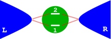
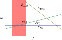
Figure 1: (color online) (LEFT) Sketch of the TLQD connected to two $s$-wave superconducting leads. (RIGHT) Energy levels $E_{Q,S;\alpha}$ of two-electron $(Q=2)$ states in the TLQD as functions of the exchange coupling $J$. The shaded region is of our interest, where the singlet-triplet transition occurs in the ground state.

The TLQD connected to two single-channel $s$-wave superconducting leads as shown in Fig. 1 is modeled by the two-impurity Anderson model: ${\mathcal{H}}={\mathcal{H}}_{\rm DD}+{\mathcal{H}}_{\rm LD}+{\mathcal{H}}_{\rm T}$, where

$${\mathcal{H}}_{\rm DD} =\sum_{i}(\epsilon_{i}n_{i}+Un_{i\uparrow}n_{i\downarrow})+Un_{1}n_{2}+J{\mathbf{S}}_{1}\cdot{\mathbf{S}}_{2}$$ (1)

$${\mathcal{H}}_{\rm LD} =\sum_{\ell{\mathbf{k}}}\left[\epsilon_{\mathbf{k}}n_{\ell{\mathbf{k}}}-\left(\Delta\,e^{i\phi_{\ell}}c_{\ell{\mathbf{k}}\uparrow}^{\dagger}c_{\ell-{\mathbf{k}}\downarrow}^{\dagger}+(h.c.)\right)\right]$$ (2)

$${\mathcal{H}}_{\rm T} =\sum_{i\ell{\mathbf{k}}\mu}\left[t_{i\ell}\,d_{i\mu}^{\dagger}c_{\ell{\mathbf{k}}\mu}+(h.c.)\right].$$ (3)

Here $c_{\ell{\mathbf{k}}\mu}$ ($d_{i\mu}$) destroys an electron with energy $\epsilon_{\mathbf{k}}$ ($\epsilon_{i}$) with respect to the fermi level and spin $\mu$ on lead $\ell=L,R$ (in orbital $i=1,2$ on the dot); $n_{\ell{\mathbf{k}}}\equiv\sum_{\mu}c_{\ell{\mathbf{k}}\mu}^{\dagger}c_{\ell{\mathbf{k}}\mu}$ and $n_{i}\equiv\sum_{\mu}d_{i\mu}^{\dagger}d_{i\mu}$ are occupation operators for the leads and the dot orbitals. The Coulomb energy of the strength $U$ is assumed to depend on the total number of electrons in the dot. The Hund’s rule in the dot results in the ferromagnetic exchange coupling denoted as $J\,(<0)$ between the electron spins ${\mathbf{S}}_{i}=\frac{1}{2}\sum_{\mu\mu^{\prime}}d_{i\mu}^{\dagger}{\boldsymbol{\sigma}}_{\mu\mu^{\prime}}d_{i\mu^{\prime}}$, where ${\boldsymbol{\sigma}}$ are Pauli matrices. The left and right leads are assumed to have identical dispersion energy $\epsilon_{\mathbf{k}}$ and superconducting gap $\Delta$, while a finite phase difference $\phi=\phi_{L}-\phi_{R}$ is applied between them. The energy-independent dot-lead tunneling amplitudes $t_{i\ell}$ hybridize the electron states between the dot and the leads, which are well characterized by tunneling rates $\Gamma_{i\ell}=\pi\rho|t_{i\ell}|^{2}$, where $\rho$ is the density of states of the leads at the Fermi energy.

Since we are interested in the regime of the singlet-triplet transition of an isolated dot, we focus on the parameter region in which the dot is doubly occupied. In addition, we consider the nondegenerate case with a finite splitting $\delta\epsilon\equiv\epsilon_{2}-\epsilon_{1}>0$ between two orbitals. Figure 1 displays the energy levels of two-electron states of the isolated dot as functions of $J$: three singlet states, $\left|2,0,0;\alpha\right\rangle$ with $\alpha=1,2,3$ and three triplet states $\left|2,1,M\right\rangle$, where the states are labeled as $\left|Q,S,M\right\rangle$ with the charge number $Q$, the spin $S$, and the $z$ component of the spin $M$. The singlet states,

$$\left|2,0,0;1\right\rangle =d_{1\uparrow}^{\dagger}d_{1\downarrow}^{\dagger}\left|0\right\rangle$$ (4a)

$$\left|2,0,0;2\right\rangle =d_{2\uparrow}^{\dagger}d_{2\downarrow}^{\dagger}\left|0\right\rangle$$ (4b)

$$\left|2,0,0;3\right\rangle =\frac{1}{\sqrt{2}}(d_{2\uparrow}^{\dagger}d_{1\downarrow}^{\dagger}-d_{2\downarrow}^{\dagger}d_{1\uparrow}^{\dagger})\left|0\right\rangle$$ (4c)

have the energies, $E_{0;1}=2\epsilon_{1}+U$, $E_{0;2}=2\epsilon_{2}+U$, $E_{0;3}=\epsilon_{1}+\epsilon_{2}+U-3J/4$, respectively, and the triplet states,

$$\left|2,1,1\right\rangle =d_{2\uparrow}^{\dagger}d_{1\uparrow}^{\dagger}\left|0\right\rangle$$ (5a)

$$\left|2,1,0\right\rangle =\frac{1}{\sqrt{2}}(d_{2\uparrow}^{\dagger}d_{1\downarrow}^{\dagger}+d_{2\downarrow}^{\dagger}d_{1\uparrow}^{\dagger})\left|0\right\rangle$$ (5b)

$$\left|2,1,-1\right\rangle =d_{2\downarrow}^{\dagger}d_{1\downarrow}^{\dagger}\left|0\right\rangle$$ (5c)

are degenerate with the energy $E_{1}=\epsilon_{1}+\epsilon_{2}+U+J/4$. Due to the finite splitting $\delta\epsilon>0$ and the existence of the inter-orbital Coulomb interaction, the singlet-triplet transition is driven by the competition between the states $\left|2,0,0;1\right\rangle$ and $\left|2,1,M\right\rangle$ [see Fig. 1]. The bare singlet-triplet splitting is then defined by

$${J_{\rm I}}^{(0)}\equiv E_{1}-E_{0;1}=\delta\epsilon+\frac{J}{4}.$$ (6)

The external gate voltage $V_{g}$ can tune the singlet-triplet splitting by affecting the level splitting $\delta\epsilon$,Kogan03 ; Holm08 the exchange coupling strength $J$,Quay07 ; Roch08 or both of them. For simplicity, we assume that the gate-voltage dependency is implemented only through $J=J(V_{g})$ and that $\delta\epsilon$ or $\epsilon_{i}$ are independent of $V_{g}$. Our simplification can still capture the main physics of the system as long as the regime close to the singlet-triplet transition is concerned.

The configuration of the dot-lead coupling is another important source that can govern the physics of the system. First, the number of the effective channels coupled to the dot can be controlled.Hofstetter02 If the condition,

$$\frac{t_{1{\rm L}}}{t_{1{\rm R}}}=\frac{t_{2{\rm L}}}{t_{2{\rm R}}}$$ (7)

is satisfied, the dot-lead coupling matrix has a zero eigenvalue, and one of the two channels can be completely decoupled from the dot under a proper unitary transformation, resulting in a one-channel problem. This reduction of the effective channels then affects the Kondo effect greatly, which will be discussed later. Secondly, the phase of the coupling coefficients has an influence on the interference and consequently on the electron transport through the dot.Rozhkov01 ; vanDam06 Even though no magnetic field is applied in our system, the (real-valued) coupling coefficients can acquire an additional phase $\pi$ depending on the parity of the orbital wave functions on the dot.vanDam06 Two distinctive cases can then be conceived: $t_{1{\rm L}}t_{1{\rm R}}t_{2{\rm L}}t_{2{\rm R}}>0$ when two orbitals have the same parity and $t_{1{\rm L}}t_{1{\rm R}}t_{2{\rm L}}t_{2{\rm R}}<0$ when they have the opposite parities. Taking into account the essential impacts of the dot-lead coupling and focusing on the consequent qualitative features of system states and electron transport, we consider two representative cases in this paper:

$$\begin{array}[]{ll}\text{case I}:&t_{1\ell}=t,~{}t_{2\ell}=\gamma t\\ \text{case II}:&t_{1\ell}=t,~{}t_{2{\rm L}}=-t_{2{\rm R}}=\gamma t\end{array}$$ (10)

with $\gamma\leq 1$. The case I deals with the effective one-channel problem with Eq. (7) satisfied, while the case II reflects the two-channel problem with the negative product of coupling coefficients. The effect of asymmetric coupling with respect to the orbitals is also examined by setting $\gamma<1$. Another kind of asymmetric junction such as $t_{i{\rm L}}\ll t_{i{\rm R}}$ that can happen frequently in realistic experimental setups like break junctionsRoch08 is not considered in our study because this asymmetry is observed to make no qualitative impact on the Josephson current.

Finally, since we are interested in the low temperature behavior, we concentrate for the most part on the Kondo regime. The hybridizations $\Gamma_{i\ell}$ are chosen to be far smaller than the particle or hole excitations with respect to the two-electron states in order to suppress the resonant tunneling. Specifically, throughout our study, we choose $\epsilon_{1}=-1.6D$, $\epsilon_{2}=-1.4D$, $U=D$, and $\Gamma=\pi\rho|t|^{2}=0.05D$, where the half band width $D$ is taken as the unit of energy. Here we have also used the particle-hole symmetry condition $\epsilon_{1}+\epsilon_{2}+3U=0$.

III Weak Coupling Limit: $\Delta\gg T_{K}$

III.1 Fourth-Order Perturbation Theory

First, we consider the weak coupling limit where the superconducting gap $\Delta$ is much larger than the Kondo temperature $T_{K}$, which will be defined in Sec. IV. In this case the supercurrent can be calculated via fourth-order perturbation theory in ${\mathcal{H}}_{\rm T}$.Rozhkov01 ; Spivak91 ; ChoiMS00 We apply degenerate perturbation theory that takes into account the singlet state $\left|2,0,0;1\right\rangle$ and the triplet states $\left|2,1,M\right\rangle$ simultaneously since they are almost degenerate close to the singlet-triplet transition point of isolated dot. Unlike the single-level quantum dot studiesRozhkov01 ; Spivak91 where it is enough to collect only terms that depend on the phase difference $\phi$, on the other hand, one must keep track of all the $\phi$-independent terms in the TLQD study because they contribute to the renormalization of the singlet-triplet splitting,ChoiMS00 and the transition point is shifted from its unnormalized position, ${J_{\rm I}}^{(0)}=0$. Due to the singlet nature of the Cooper pair, there exists no coupling between the singlet and the triplet states to any order of the perturbation, and the energy of each state is separately shifted: $E_{a}=E_{a}^{(0)}+\delta E_{a}(\phi)$ for $a=S,T$ with $E_{S}^{(0)}=E_{0;1}$ and $E_{T}^{(0)}=E_{1}$. The energy shifts are given by

$$\delta E_{a} =\beta_{a0}\Gamma\sum_{i\ell}\gamma_{i\ell}^{2}+\frac{\Gamma^{2}}{\Delta}\Big{[}\beta_{a1}\sum_{i\ell}\gamma_{i\ell}^{4}+\beta_{a2}\sum_{\ell}\gamma_{1\ell}^{2}\gamma_{2\ell}^{2}$$

$$\quad\mbox{}+\beta_{a3}\sum_{\ell\neq\ell^{\prime}}\gamma_{1\ell}^{2}\gamma_{2\ell^{\prime}}^{2}+(\beta_{a4}-\beta^{\prime}_{a4}\cos\phi)\sum_{i}\gamma_{i{\rm L}}^{2}\gamma_{i{\rm R}}^{2}$$

$$\quad\mbox{}+(\beta_{a5}-\beta^{\prime}_{a5}\cos\phi)\gamma_{1{\rm L}}\gamma_{1{\rm R}}\gamma_{2{\rm L}}\gamma_{2{\rm R}}\Big{]},$$ (11)

where we have defined $\gamma_{i\ell}\equiv t_{i\ell}/t$. Figure 2 shows typical virtual hopping processes that contribute to each term in Eq. (11). The detailed expressions for the coefficients $\beta_{ai}$ can be found in the Appendix.

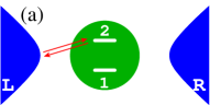
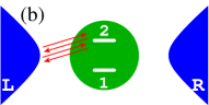
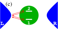
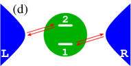
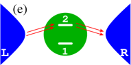
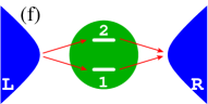
Figure 2: (color online) Listing of typical virtual tunneling processes contributing to $\delta E_{a}$. The arrows indicate the direction of the charge transfers for processes contributing to (a) $\beta_{a0}$, (b) $\beta_{a1}$, (c) $\beta_{a2}$, (d) $\beta_{a3}$, (e) $\beta^{(\prime)}_{a4}$, and (f) $\beta^{(\prime)}_{a5}$.

The effective singlet-triplet splitting then becomes

$${J_{\rm I}}(\phi)=E_{T}(\phi)-E_{S}(\phi)={J_{\rm I}}^{(0)}+\delta{J_{\rm I}}(\phi)$$ (12)

with

$$\delta{J_{\rm I}}\equiv\delta E_{T}-\delta E_{S}\equiv\delta{J_{\rm I}}^{(2)}+\delta{J_{\rm I}}^{(4)},$$ (13)

where $\delta{J_{\rm I}}^{(2)}$ and $\delta{J_{\rm I}}^{(4)}$ consist of the terms that are proportional to $\Gamma$ and $\Gamma^{2}$, respectively. We find that $\delta{J_{\rm I}}$ is mostly positive in the parameter regime of our interest, favoring the singlet formation. The singlet-triplet transition point $J_{c}$ when ${J_{\rm I}}(J=J_{c})=0$, which now becomes $\phi$-dependent, is then shifted from its bare value $J_{c}^{(0)}=-4\delta\epsilon=-0.8D$ to a more negative value. It should be noted that the second-order contribution to $\delta{J_{\rm I}}$

$$\delta{J_{\rm I}}^{(2)}=(\beta_{T0}-\beta_{S0})\Gamma\sum_{i\ell}\gamma_{i\ell}^{2}$$ (14)

is finite in contrast to the previous study of parallel double-dot systemChoiMS00 where the leading contribution is found to be of the order of $\Gamma^{2}$. The main difference comes from the characteristics of the singlet states in two systems. In the double-dot system studied by Choi et al., the two quantum dots, each of which is singly occupied, are identical and have no Coulomb interaction between them so the lowest-lying singlet state is $\left|2,0,0;3\right\rangle$, while it is $\left|2,0,0;1\right\rangle$ in our system due to the existence of the finite splitting and the inter-orbital Coulomb interaction. The singlet state $\left|2,0,0;3\right\rangle$ has the same charge distribution as the triplet states $\left|2,1,M\right\rangle$, so the second-order perturbation does not give rise to any additional splitting between two states [see Fig. 2 (a)]. On the other hand, having $\left|2,0,0;1\right\rangle$ as the lowest-lying singlet states, our system can exhibit a rather huge renormalization of the singlet-triplet splitting that is of the order of $\Gamma$. This second-order term $\delta{J_{\rm I}}^{(2)}$ is numerically found to increase as $\Delta$ is decreased. This tendency is opposite to the expectation that the renormalization, which is due to the tunneling of Cooper pairs whose amplitude increases with $\Delta$, should be weakened as $\Delta$ decreases: in other words, $\lim_{\Delta\to 0}\delta{J_{\rm I}}=0$. This discrepancy should be resolved by the higher-order terms of the order of $(\Gamma/\Delta)^{n}$ that are more involved as $\Delta$ decreases: In fact, the fourth-order term $\delta{J_{\rm I}}^{(4)}$ is observed to become negative for smaller $\Delta$ so that the renormalization is diminished. Owing to this opposite $\Delta$-dependencies of $\delta{J_{\rm I}}^{(2)}$ and the other higher-order terms, ${J_{\rm I}}$ varies non-monotonically with $\Delta$, which in turns implies that the transition point $J_{c}$ also displays a non-monotonic dependency on $\Delta$: see Figs. 3 and 5.

The supercurrent can be calculated via the derivative of the energy with respect to the phase difference $\phi$:

$$I_{a}=\frac{2e}{\hbar}\frac{\partial E_{a}}{\partial\phi}=\hat{I}_{a}\sin\phi$$ (15)

with

$$\frac{\hat{I}_{a}}{I_{c}^{\rm short}}=2\left(\frac{\Gamma}{\Delta}\right)^{2}\!\!\left(\beta^{\prime}_{a4}\sum_{i}\gamma_{i{\rm L}}^{2}\gamma_{i{\rm R}}^{2}+\beta^{\prime}_{a5}\gamma_{1{\rm L}}\gamma_{1{\rm R}}\gamma_{2{\rm L}}\gamma_{2{\rm R}}\right)$$ (16)

As a matter of fact, only the virtual processes in Figs. 2 (e) and (f) contribute to the Cooper pair tunneling. The $\beta^{\prime}_{a4}$-term [(e)] arises from the diagonal processes where both electrons in a Cooper pair travel through either the orbital 1 or 2, while the $\beta^{\prime}_{a5}$-term [(f)] from the off-diagonal processes with one electron traveling through the orbital 1 and the other traveling through the orbital 2. Depending on the order of the sequence of electron tunneling and the spin correlation of dot electrons, the coefficients $\beta^{\prime}_{ai}$ can acquire a relative minus sign owing to Fermi statistics. For the singlet state, one can find that

$$\beta^{\prime}_{S4}>0\quad\text{and}\quad\beta^{\prime}_{S5}<0.$$ (17)

The negative sign for $\beta^{\prime}_{S5}$ is attributed to the processes with one electron traveling through a filled level (orbital 1) and the other electron through an empty level (orbital 2). It should be noted that it is necessary to take into account the dot electron correlation exactly in order to determine the supercurrent sign correctly. Not all the processes contributing to $\beta^{\prime}_{S5}$ acquire the $\pi$ phase: For example, the processes with the intermediate state $\left|2,0,0;3\right\rangle$ acquire no phase at all [see Eq. (78)], while their amplitudes are always smaller than those of the other processes, and finally $\beta^{\prime}_{S5}$ is negative. For the triplet state,

$$\beta^{\prime}_{T4}<0\quad\text{and}\quad\beta^{\prime}_{T5}<0$$ (18)

because of the presence of local magnetic moments in both orbitals.Spivak91 Apart from the sign, we have found numerically that the off-diagonal processes usually have larger amplitude than the diagonal ones:

$$2|\beta^{\prime}_{a4}|<|\beta^{\prime}_{a5}|\qquad\text{for}\ a=S,T.$$ (19)

Hence, when the product $\gamma_{1{\rm L}}\gamma_{1{\rm R}}\gamma_{2{\rm L}}\gamma_{2{\rm R}}$ is comparable to $\sum_{i}\gamma_{i{\rm L}}^{2}\gamma_{i{\rm R}}^{2}$ in magnitude, the sign of the supercurrent dictates the sign of the off-diagonal term, or that of the product $-\gamma_{1{\rm L}}\gamma_{1{\rm R}}\gamma_{2{\rm L}}\gamma_{2{\rm R}}$ regardless of the spin state: the current exhibits the 0($\pi$)-junction for the negative (positive) product. Otherwise, that is, if $|\gamma_{1{\rm L}}\gamma_{1{\rm R}}\gamma_{2{\rm L}}\gamma_{2{\rm R}}|\ll\sum_{i}\gamma_{i{\rm L}}^{2}\gamma_{i{\rm R}}^{2}$, the diagonal term prevails in determining the sign of the supercurrent so that the singlet (triplet) state features the 0($\pi$)-junction behavior regardless of the sign of the product.

In the following sections, we identify the system state according to its ground-state spin and the sign of the supercurrent in the $\Delta$-$J$ plane. We use the labels $S$ and $T$ to denote the spin singlet and triplet state, respectively. Since the phase transition depends on the superconducting phase difference $\phi$ as well, the phase boundaries are located at three different values of $\phi$: 0 (red line), $\pi/2$ (green line), and $\pi$ (blue line). Between $\phi=0$ and $\pi$ boundaries the system is in the intermediate state having a stable ground state and a meta-stable state. The intermediate states are tagged with a subscript that represents the meta-stable state spin. For example, the ground state in the state $T_{S}$ is mostly of the spin triplet, while it is of the spin singlet at and near $\phi=0$, and the system experiences a phase transition from spin doublet to singlet as $\phi$ is varied from 0 to $\pi$. The state identification is then supplemented by the SPR calculated from Eq. (16), classifying whether it is of either $0^{(\prime)}$ or $\pi^{(\prime)}$ junctions. Two states with same ground-state spin can be distinguished if their SPRs are different and the boundary between them will be colored in yellow line.

III.2 Case I: $\gamma_{1{\rm L}}\gamma_{1{\rm R}}\gamma_{2{\rm L}}\gamma_{2{\rm R}}>0$

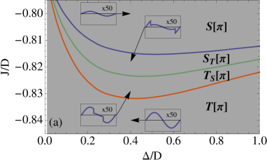
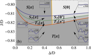
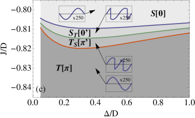
Figure 3: (color online) Phase diagrams in the $\Delta$-$J$ plane for the case I with $\gamma=1$ [(a)], 0.6 [(b)], and 0.1 [(c)]. The phase boundaries are located when the ground-state spin is changed at $\phi=0$ (red line), $\pi/2$ (green line), and $\pi$ (blue line). The yellow line separates two states with same ground-state spin but different SPRs. Each phase is shaded in gray scale according to its SPR: lighter gray for 0 junction and darker gray for $\pi$ junction. Refer the detailed classification of the states to the text. The insets show the SPR for $\phi\in[-\pi,\pi]$ at the points indicated by the arrows. Here the value of $\Delta$ is swept from $\Gamma$ to $D$, and for $\Delta<\Gamma$ the above diagrams are not valid.

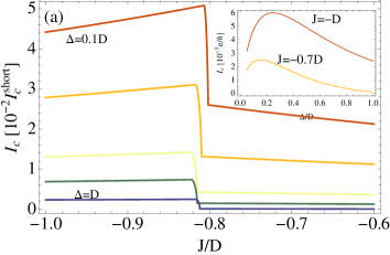
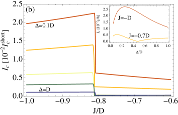
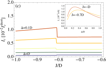
Figure 4: (color online) Critical currents as functions of $J$ in units of $I_{c}^{\rm short}$ for the case I with $\gamma=1$ [(a)], 0.6 [(b)], and 0.1 [(c)] for various values of $\Delta$: $0.1D$ (top), $0.2D$, $0.4D$, $0.6D$, and $D$ (bottom). The insets display the critical currents as functions of $\Delta$ in units of $e/\hbar$ for $J=-0.7D$ (in the spin triplet state) and $-D$ (in the spin singlet state).

Figure 3 shows the phase diagrams in the $\Delta$-$J$ plane in the case I for various values of $\gamma$. The lower bound of $\Delta$ is set to $\Gamma$ because the perturbation theory works only when $\Gamma\ll\Delta$. For $\gamma=1$, the Josephson coupling

$$\frac{\hat{I}_{a}}{I_{c}^{\rm short}}=2(\Gamma/\Delta)^{2}(2\beta^{\prime}_{a4}+\beta^{\prime}_{a5})$$ (20)

is always negative because $\beta^{\prime}_{a5}<0$ and $2|\beta^{\prime}_{a4}|<|\beta^{\prime}_{a5}|$, and the current exhibits the $\pi$-junction behavior, no matter what values $J$ and $\Delta$ have [see Fig. 3 (a)]. For $\gamma\ll 1$, on the other hand, the contribution from the off-diagonal term becomes negligible since

$$\gamma^{2}=\gamma_{1{\rm L}}\gamma_{1{\rm R}}\gamma_{2{\rm L}}\gamma_{2{\rm R}}\ll\sum_{i}\gamma_{i{\rm L}}^{2}\gamma_{i{\rm R}}^{2}=1+\gamma^{4},$$ (21)

and the sign of $\hat{I}_{a}$ is governed solely by the $\beta^{\prime}_{a4}$ term. The spin singlet state is then of the 0 junction since $\beta^{\prime}_{S4}>0$, and the singlet-triplet transition accompanies the 0-$\pi$ transition with the intermediate states as shown in Fig. 3 (c). Figure 3 (b) shows that for intermediate values of $\gamma$, both of the 0 and $\pi$ junctions can appear in the spin singlet state: the 0 and $\pi$ junctions take place in the regions with larger and smaller values of $\Delta$, respectively. The phase boundary separating two regions moves toward the smaller $\Delta$ as $\gamma$ is decreased.

Different strength of the Josephson coupling in the spin singlet and triplet states gives rise to a discontinuous change in the SPR in the intermediate states [see the insets in Fig. 3] and a rapid change in the critical current $I_{c}\equiv|\hat{I}_{a}|$ across the singlet-triplet transition as shown in Fig. 4. The numerical calculation of the supercurrent finds that the supercurrent is stronger in the spin triplet state than in the spin singlet state: $|\hat{I}_{T}|>|\hat{I}_{S}|$. In the spin singlet state the diagonal and the off-diagonal processes make the opposite contributions ($\beta^{\prime}_{S4}>0>\beta^{\prime}_{S5}$), resulting in a partial cancellation. This is not the case in the spin triplet state in which both processes contribute to the $\pi$ junction ($\beta^{\prime}_{T4},\beta^{\prime}_{T5}<0$). For small $\gamma$, on the other hand, such a cancellation does not make a significant role since the $\beta^{\prime}_{a5}$ term becomes much smaller than the $\beta^{\prime}_{a4}$ term, so the critical currents in both spin states become comparable as can be seen in Fig. 4 (c).

The critical current exhibits a non-monotonic dependence on $\Delta$: see the insets in Fig. 4. In two extreme limits, $\Delta\ll\Gamma$ and $\Delta\gg\Gamma$, the supercurrent should vanish. The supercurrent, induced by the proximity effect that is proportional to $\Delta$, should vanish in the limit $\Delta\to 0$. In the opposite limit, the high energy cost $\sqrt{\Delta^{2}+\epsilon_{\mathbf{k}}^{2}}$ of the quasiparticles created during the virtual processes suppresses the current. Consequently, the critical current has a maximum as a function of $\Delta$. For the intermediate values of $\gamma$ when the 0-$\pi$ transition occur in the spin singlet state, the critical current can become zero at the transition [see the inset in Fig. 4 (b)].

III.3 Case II: $\gamma_{1{\rm L}}\gamma_{1{\rm R}}\gamma_{2{\rm L}}\gamma_{2{\rm R}}<0$

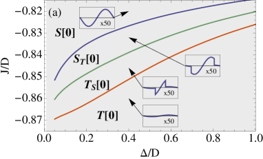
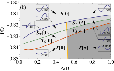
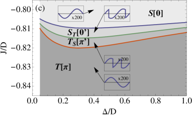
Figure 5: (color online) Phase diagrams in the $\Delta$-$J$ plane for the case II with $\gamma=1$ [(a)], 0.72 [(b)], and 0.1 [(c)]. Refer to Fig. 3 for the details.

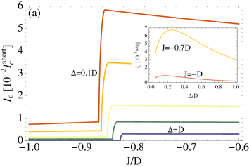
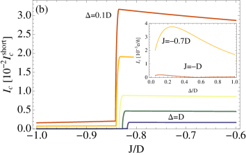
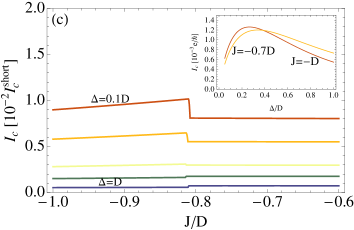
Figure 6: (color online) Critical currents as functions of $J$ in units of $I_{c}^{\rm short}$ for the case II with $\gamma=1$ [(a)], 0.72 [(b)], and 0.1 [(c)] for various values of $\Delta$: $0.1D$ (top), $0.2D$, $0.4D$, $0.6D$, and $D$ (bottom). Refer the guide for the insets to Fig. 5.

The phase diagram and the critical current in the case II are shown in Figs. 5 and 6, respectively. In this case one of the dot-lead tunneling amplitude changes its sign, making the product $\gamma_{1{\rm L}}\gamma_{1{\rm R}}\gamma_{2{\rm L}}\gamma_{2{\rm R}}$ negative and accordingly reversing the sign of the off-diagonal contributions. It then switches the junction characteristics from $\pi$ to 0 junction for the case $\gamma=1$ when the off-diagonal term prevail over the diagonal term: compare Fig. 3 (a) and Fig. 5 (a). However, for $\gamma\ll 1$ when the off-diagonal contributions are negligible, the negative product does not affect the supercurrent and the phase diagram so much: Fig. 3 (c) and Fig. 5 (c) are almost identical. As a result, for the intermediate values of $\gamma$, the additional 0-$\pi$ transition now takes place in the spin triplet state in contrast to the case I: compare Fig. 3 (b) and Fig. 5 (b). Another difference from the case I is that the critical current is now much larger in the spin singlet state than in the spin triplet state as long as $\gamma$ is not so small: see Fig. 6. The same argument used in the case I applies as well: With the negative product, the $\beta^{\prime}_{T4}$ term which is negative cuts down the positive contribution from the $\beta^{\prime}_{T5}$ term, while in the spin singlet state both of two terms contributes to the 0 junction.

In addition to the properties of the supercurrent, the shape of the phase boundaries are also different from those in the case I. Figures 5 (a) and (b) show that for the moderate values of $\gamma$ the phase boundaries are much shifted toward the spin triplet side, implying that the spin singlet state is being further favored. Furthermore, the transition point $J_{c}$ displays a monotonic dependence on $\Delta$ and does not approach its bare value in the limit $\Delta\to 0$, which is contradictory to our expectation from the previous weak-coupling argument. The inclination to the spin singlet state is accounted for by looking at the $\beta_{a5}$ term in $\delta E_{a}$ that is proportional to $\gamma_{1{\rm L}}\gamma_{1{\rm R}}\gamma_{2{\rm L}}\gamma_{2{\rm R}}$ [see the last term in Eq. (11)]. Numerical calculations observe $\beta_{S5}>0$ and $|\beta_{S5}|>|\beta_{\rm T5}|$, which means that with the negative product $\gamma_{1{\rm L}}\gamma_{1{\rm R}}\gamma_{2{\rm L}}\gamma_{2{\rm R}}<0$ the spin singlet state is much lowered than the spin triplet state [see the Appendix for expressions of $\beta_{S5}$ and $\beta_{T5}$]. This term is also observed to make the fourth-order splitting term $\delta{J_{\rm I}}^{(4)}$ positive, which is the cause of the monotonic behavior of $J_{c}$. One may suspect that this favoring of the spin singlet state in the limit $\Delta\to 0$ is the artifact of the fourth-order perturbation close to its limit of validity, $\Gamma/\Delta\sim 1$. However, the non-perturbative NRG study in the following section finds that the system should be of the spin singlet state in the vanishing $\Delta$ limit and that it is attributed to the complete screening of dot spins by the two-channel conduction electrons, which will be discussed in details in the next section. Considering that the Kondo effect which is responsible for the screening cannot be correctly captured by the perturbation theory, it is quite interesting that it still reflects correct asymptotic behaviors in the limit $\Delta\to 0$: the approaching of $J_{c}$ to its bare value in the case I and the precursor of the disappearance of the spin triplet state in the case II.

IV Strong Coupling Limit: $\Delta\ll T_{K}$

In this section we extend our study to the strong-coupling limit by using the NRG method that is known to be suitable for the non-perturbative study of the low-temperature properties of the impurity system. Even though the standard NRG procedureWilson75 can be directly applied to the original Hamiltonian, we have introduced a unitary transformation

$$\begin{bmatrix}c_{a{\mathbf{k}}\mu}\\ c_{b{\mathbf{k}}\mu}\end{bmatrix}={\mathcal{S}}\begin{bmatrix}c_{{\rm L}{\mathbf{k}}\mu}\\ c_{{\rm R}{\mathbf{k}}\mu}\end{bmatrix},\ \begin{bmatrix}d_{a\mu}\\ d_{b\mu}\end{bmatrix}={\mathcal{D}}\begin{bmatrix}d_{1\mu}\\ d_{2\mu}\end{bmatrix}$$ (22)

which makes all the matrix elements of the Hamiltonian real in order to boost up the speed of the numerical computation. Here the unitary matrices are chosen to be

$${\mathcal{S}}=\frac{1}{\sqrt{2}}\begin{bmatrix}ie^{-i\phi/4}&-ie^{+i\phi/4}\\ e^{-i\phi/4}&e^{+i\phi/4}\end{bmatrix},\ {\mathcal{D}}=\begin{bmatrix}1&0\\ 0&\chi\end{bmatrix},$$ (23)

where $\chi=1$ and $i$ in the cases I and II, respectively. Under the unitary transformation, each part of the Hamiltonian is transformed into

$${\mathcal{H}}^{\prime}_{\rm DD} =\sum_{s=a,b}(\epsilon_{s}n_{s}+Un_{s\uparrow}n_{s\downarrow})+Un_{a}n_{b}+J{\mathbf{S}}_{a}\cdot{\mathbf{S}}_{b}$$ (24)

$${\mathcal{H}}^{\prime}_{\rm LD} =\sum_{s{\mathbf{k}}}\left[\epsilon_{\mathbf{k}}n_{s{\mathbf{k}}}-(-1)^{s}\Delta\left(c_{s{\mathbf{k}}\uparrow}^{\dagger}c_{s-{\mathbf{k}}\downarrow}^{\dagger}{+}(h.c.)\right)\right]$$ (25)

$${\mathcal{H}}^{\prime}_{\rm T} =\sum_{ss^{\prime}{\mathbf{k}}\mu}\left[t_{ss^{\prime}}\,d_{s\mu}^{\dagger}c_{s^{\prime}{\mathbf{k}}\mu}+(h.c.)\right],$$ (26)

respectively, where $(-1)^{a}=-1$ and $(-1)^{b}=1$. Here the transformed dot-lead coupling matrix is given by

$$\begin{bmatrix}t_{aa}&t_{ab}\\ t_{ba}&t_{bb}\end{bmatrix}=\begin{cases}\displaystyle\sqrt{2}t\begin{bmatrix}\sin\frac{\phi}{4}&\cos\frac{\phi}{4}\\ \gamma\sin\frac{\phi}{4}&\gamma\cos\frac{\phi}{4}\end{bmatrix},&\text{case I}\\ \displaystyle\sqrt{2}t\begin{bmatrix}\sin\frac{\phi}{4}&\cos\frac{\phi}{4}\\ \gamma\cos\frac{\phi}{4}&-\gamma\sin\frac{\phi}{4}\end{bmatrix},&\text{case II}\end{cases}$$ (27)

The Wilson’s NRG techniqueWilson75 ; Krishnamurthy80 consists of the logarithmic discretization of the conduction bands, the mapping onto a semi-infinite chain, and the iterative diagonalization of the properly truncated Hamiltonian. Following the standard NRG procedures extended to superconducting leads,Yoshioka00 we evaluate various physical quantities from the recursion relation

$$\widetilde{{\mathcal{H}}}_{N+1} =\sqrt{\Lambda}\widetilde{{\mathcal{H}}}_{N}+\xi_{N}\sum_{s\mu}(f_{sN\mu}^{\dagger}f_{sN{+}1\mu}+(h.c.))$$

$$\quad\mbox{}-\sum_{s}(-1)^{s}\widetilde{\Delta}(f_{sN{+}1\uparrow}^{\dagger}f_{sN{+}1\downarrow}^{\dagger}+(h.c.))$$ (28)

for $N\geq 0$ with the initial Hamiltonian given by

$$\widetilde{{\mathcal{H}}}_{0} =\frac{1}{\sqrt{\Lambda}}\Bigg{[}\widetilde{{\mathcal{H}}}_{\rm D}+\sum_{ss^{\prime}}\sqrt{\widetilde{\Gamma}_{ss^{\prime}}}\sum_{\mu}(d_{s\mu}^{\dagger}f_{s^{\prime}0\mu}+(h.c.))$$

$$\qquad\qquad\mbox{}-\sum_{s\mu}(-1)^{s}\widetilde{\Delta}(f_{s0\uparrow}^{\dagger}f_{s0\downarrow}^{\dagger}+(h.c.))\Bigg{]}.$$ (29)

Here the fermion operators $f_{sN\mu}$ have been introduced as a result of the logarithmic discretization of the conduction bands and the accompanying tridiagonalization, $\Lambda$ is the logarithmic discretization parameter (we choose $\Lambda=4$), and

$$\xi_{N} =\frac{1-\Lambda^{-(N+1)}}{\sqrt{(1-\Lambda^{-(2N+1)})(1-\Lambda^{-(2N+3)})}},$$ (30)

$$\widetilde{{\mathcal{H}}}_{\rm D} =\frac{{\mathcal{H}}^{\prime}_{\rm D}}{{\mathcal{E}}D},\quad\widetilde{\Delta}=\frac{\Delta}{{\mathcal{E}}D},\quad\sqrt{\widetilde{\Gamma}_{ss^{\prime}}}=\frac{1}{{\mathcal{E}}}\sqrt{\frac{2\Gamma}{\pi D}}\frac{t_{ss^{\prime}}}{t}$$ (31)

with ${\mathcal{E}}=(1+\Lambda^{-1})/2$. The original Hamiltonian is recovered by

$$\frac{{\mathcal{H}}^{\prime}}{D}=\lim_{N\to\infty}{\mathcal{E}}\Lambda^{-(N-1)/2}\widetilde{{\mathcal{H}}}_{N}.$$ (32)

It has been knownKrishnamurthy80 ; Campo05 that the logarithmic discretization underestimates the coupling between the conduction-band electrons and the dot electrons. In order to avoid this problem, we multiply $\widetilde{\Gamma}$ by a correction factor $A_{\Lambda}$ given byKrishnamurthy80 ; Campo05

$$A_{\Lambda}=\frac{\ln\Lambda}{2}\frac{\Lambda+1}{\Lambda-1}.$$ (33)

Within the NRG procedure, the spin of the ground state, the occupation $\left\langle n_{i}\right\rangle$, and the spin correlation $\left\langle{\mathbf{S}}_{1}\cdot{\mathbf{S}}_{2}\right\rangle$ can be directly calculated from the expectation values of the corresponding operators. The supercurrent can be also obtained by calculating the expectation value

$$I=\frac{e}{2}\left\langle\dot{N}_{L}-\dot{N}_{R}\right\rangle,$$ (34)

where $N_{\ell}=\sum_{\mathbf{k}}n_{\ell{\mathbf{k}}}$. In terms of the fermion operators $f_{s0\mu}$, the current expectation value is expressed as

$$\frac{I}{I_{c}^{\rm short}}=\frac{D}{\Delta}\sqrt{\frac{2\Gamma}{\pi D}}\sum_{ss^{\prime}\mu}\left\langle i_{ss^{\prime}}d_{s\mu}^{\dagger}f_{s^{\prime}0\mu}+(h.c.)\right\rangle$$ (35)

with the current matrix defined by

$$\begin{bmatrix}i_{aa}&i_{ab}\\ i_{ba}&i_{bb}\end{bmatrix}=\frac{1}{2t}\begin{bmatrix}t_{ab}&-t_{aa}\\ t_{bb}&-t_{ba}\end{bmatrix}.$$ (36)

The Andreev levels are located from the subgap many-body excitations which are identified as the poles of the dot Green’s functions.

IV.1 Normal Leads: $\Delta=0$

In the presence of Coulomb interaction and spin exchange coupling, strong dot-lead coupling can induce nontrivial many-body correlations that may compete with and even suppress superconductivity. A promising candidate of such many-body correlations in the QD system is the Kondo effect. In order to identify nontrivial correlations in our system and to elaborate the analysis of the strongly-coupled Josephson junction, it is quite useful to investigate the normal-lead case with $\Delta=0$. The NRG procedure described above is then applied by setting $\Delta=0$ and $\phi=0$: The latter condition, though not being essential, is imposed in order to simplify the dot-lead coupling matrix [Eq. (27)]. The normal-lead version of our system has been well studied in the literature, so we briefly summarize the known theoretical analyses and present relevant numerical results in our parameter regime for comparison with the superconducting case.

IV.1.1 Case I: Single Channel

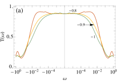
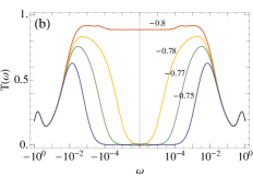
Figure 7: (color online) Energy-resolved transmission coefficient $T(\omega)$ for a two-level QD coupled to normal leads (case I) with ferromagnetic $({J_{\rm I}}<J_{c})$ [(a)] and antiferromagnetic $({J_{\rm I}}>J_{c})$ [(b)] exchange coupling for various values of $J/D$ (as annotated).

In the case I only the lead-$b$, that is, the symmetrized conduction-band channel is coupled to the dot, with the other channel completely detached: see Eq. (27). The two-level QD system attached to a single conduction channel has been well studied in the context of the quantum phase transition in a vicinity of singlet-triplet degenerate point.Hofstetter02 In this case the system can be mapped onto an exchange-coupled $S=1/2$ Kondo model through a Schrieffer-Wolff transformation:Schrieffer66

$${\mathcal{H}}_{\rm eff}={\mathcal{H}}_{\rm LD}+J_{a}\,\widetilde{\mathbf{S}}_{a}\cdot{\mathbf{s}}_{bb}+J_{b}\,\widetilde{\mathbf{S}}_{b}\cdot{\mathbf{s}}_{bb}+{J_{\rm I}}\,\widetilde{\mathbf{S}}_{a}\cdot\widetilde{\mathbf{S}}_{b}\,.$$ (37)

Here the Kondo spins $\widetilde{\mathbf{S}}_{a}$ and $\widetilde{\mathbf{S}}_{b}$ are fictitious QD spins defined on the basis of the spin singlet state $\left|2,0,0;1\right\rangle$ and the spin triplet states $\left|2,1,M\right\rangle$. Both of the Kondo spins are coupled to the localized spin of the conduction channel ${\mathbf{s}}_{bb}$ associated to the symmetrized combination of left and right leads [see Eq. (23)]: Here we define the localized spins of conduction-band electron spins as

$${\mathbf{s}}_{ss^{\prime}}\equiv\frac{1}{2}\sum_{{\mathbf{k}}{\mathbf{k}}^{\prime}}\sum_{\mu\mu^{\prime}}c_{s{\mathbf{k}}\mu}^{\dagger}{\boldsymbol{\sigma}}_{\mu\mu^{\prime}}c_{s^{\prime}{\mathbf{k}}^{\prime}\mu^{\prime}}.$$ (38)

The effective spin couplings are, up to linear order in $\Gamma$,

$$J_{a/b} =\frac{2\Gamma}{\pi\rho}\left(\frac{\gamma^{2}\mp\sqrt{2}\gamma}{-\epsilon_{2}-U-J/4}+\frac{1\mp\sqrt{2}\gamma}{\epsilon_{1}+2U-J/4}+\frac{1}{-\epsilon_{1}-U-J/4}+\frac{\gamma^{2}}{\epsilon_{2}+2U-J/4}\right)$$ (39a)

$${J_{\rm I}} =\delta\epsilon+\frac{J}{4}+\frac{4D\Gamma}{\pi}\left(\frac{2}{-\epsilon_{1}-U}-\frac{\gamma^{2}}{-\epsilon_{2}-U-J/4}-\frac{1}{-\epsilon_{1}-U-J/4}\right).$$ (39b)

Note that one has $J_{a}\neq J_{b}$ as long as $\gamma\neq 0$.

The ground state of the Kondo Hamiltonian, Eq. (37) can be of the spin singlet or doublet depending on the strength of the effective exchange coupling ${J_{\rm I}}$ and is known to undergo a phase transition at the critical coupling ${J_{\rm I}}=J_{c}$, which is of the Kosterlitz-Thouless-type.Vojta02 The ferromagnetic side $({J_{\rm I}}<J_{c})$ corresponds to an underscreened $S=1$ Kondo model where the conduction electrons screen one of the Kondo spins and the remaining $S=1/2$ spin then couples ferromagnetically to the conduction band and becomes asymptotically free at low energies.Cragg79 The corresponding Kondo temperature $T_{K}(J)$ decreases with increasing $|\Delta J|\equiv|{J_{\rm I}}-J_{c}|$ [see Fig. 7 (a)]. On the other hand, on the antiferromagnetic side $({J_{\rm I}}>J_{c})$, a two-stage Kondo effect takes place for small $\Delta J$.Hofstetter02 ; SCQD ; vanderWiel02 First, the Kondo effect leads to a screening of one of the Kondo spins, ${\mathbf{S}}_{a}$ with the larger coupling (for example we assume $J_{a}>J_{b}$) which therefore defines the larger Kondo temperature $T_{K}$. For temperatures lower than $T_{K}$, the second spin ${\mathbf{S}}_{b}$ is decoupled from the conduction band. At a much lower energy scale (denoted as $T_{K}^{I}$), the effective antiferromagnetic exchange coupling ${J_{\rm I}}$ between ${\mathbf{S}}_{a}$ and ${\mathbf{S}}_{b}$ then induces the second screening due to the local Fermi liquid that is formed on the first spin. $T_{K}^{I}$ is then the Kondo temperature of the second spin screened by electrons of a bandwidth $\sim T_{K}$ and density of states $\sim 1/(\pi T_{K})$:Hofstetter02 ; SCQD

$$T_{K}^{I}\sim T_{K}\exp\left[-\pi\frac{T_{K}}{\Delta J}\right].$$ (40)

The second Kondo effect leads to a Fano resonance and makes a dip in the energy-resolved transmission coefficientHofstetter02

$$T(\omega)=-\sum_{ii^{\prime}\mu}\frac{\Gamma}{2}\gamma_{i^{\prime}i}{\rm Im}G_{ii^{\prime}\mu}(\omega),$$ (41)

where we have introduced the retarded QD Green’s functions $G_{ii^{\prime}\mu}(t)=-i\Theta(t)\mathinner{\langle{\textstyle\{d_{i\mu}(t),d_{i^{\prime}\mu}^{\dagger}\}}\rangle}$ and a coupling matrix $\gamma_{ii^{\prime}}$ with $\gamma_{11}=1$, $\gamma_{12}=\gamma_{21}=\gamma$, and $\gamma_{22}=\gamma^{2}$. As shown in Fig. 7 (b), the dip becomes widened with increasing $\Delta J$ and eventually overrides the Kondo peak until $T_{K}^{I}\approx T_{K}$ at which the Kondo effect completely vanishes.

IV.1.2 Case II: Two Channels

Unless the zero-eigenvalue condition, Eq. (7) is satisfied, the dot is always coupled to both of the two conduction-band channels. The low-energy physics of the system is then governed by the two-channel two-impurity Kondo model with an exchange coupling. Similarly to the case I, the effective spin model can be derived via the Schrieffer-Wolff transformation:

$${\mathcal{H}}_{\rm eff} ={\mathcal{H}}_{\rm LD}+\widetilde{\mathbf{S}}_{a}\cdot\left(J_{a}\,{\mathbf{s}}_{aa}+J_{b}\,{\mathbf{s}}_{bb}+J_{ab}({\mathbf{s}}_{ab}+{\mathbf{s}}_{ba})\right)$$

$$\quad\mbox{}+\widetilde{\mathbf{S}}_{b}\cdot\left(J_{a}\,{\mathbf{s}}_{aa}+J_{b}\,{\mathbf{s}}_{bb}-J_{ab}({\mathbf{s}}_{ab}+{\mathbf{s}}_{ba})\right)$$

$$\quad\mbox{}+{J_{\rm I}}\,\widetilde{\mathbf{S}}_{a}\cdot\widetilde{\mathbf{S}}_{b}+2iJ_{ab}(\widetilde{\mathbf{S}}_{a}\times\widetilde{\mathbf{S}}_{b})\cdot({\mathbf{s}}_{ab}-{\mathbf{s}}_{ba}).$$ (42)

The exchange coupling coefficients are given by

$$J_{a} =\frac{2\Gamma}{\pi\rho}\left(\frac{1}{\epsilon_{1}+2U-J/4}{+}\frac{1}{-\epsilon_{1}-U-J/4}\right)$$ (43a)

$$J_{b} =\frac{2\gamma^{2}\Gamma}{\pi\rho}\left(\frac{1}{-\epsilon_{2}-U-J/4}{+}\frac{1}{\epsilon_{2}+2U-J/4}\right)$$ (43b)

$$J_{ab} =\frac{\sqrt{2}\gamma\Gamma}{\pi\rho}\left(\frac{1}{-\epsilon_{2}-U-J/4}{+}\frac{1}{\epsilon_{1}+2U-J/4}\right),$$ (43c)

while one obtains the same expression for ${J_{\rm I}}$ as Eq. (39b). Here each of two Kondo spins is coupled to composite localized spins of conduction-band channels. The effective Hamiltonian, Eq. (42) is not convenient for further analysis since it contains cross terms (${\mathbf{s}}_{ab}$ and ${\mathbf{s}}_{ba}$) that do not conserve the channel degrees of freedom. We introduce a unitary transformations that diagonalizes the conduction-band spin operator in the channel basis that is coupled to $\widetilde{\mathbf{S}}_{q}$ for $q=a,b$:

$$\begin{bmatrix}\tilde{c}_{a{\mathbf{k}}\mu}\\ \tilde{c}_{b{\mathbf{k}}\mu}\end{bmatrix}=\begin{bmatrix}\cos\vartheta&\sin\vartheta\\ -\sin\vartheta&\cos\vartheta\end{bmatrix}\begin{bmatrix}c_{a{\mathbf{k}}\mu}\\ c_{b{\mathbf{k}}\mu}\end{bmatrix}$$ (44)

with $\vartheta\equiv\pm\frac{1}{2}\tan^{-1}[2J_{ab}/(J_{a}{-}J_{b})]$ for $q=a$ (upper sign) and $b$ (lower sign), respectively. In terms of rotated conduction-band spins $\widetilde{\mathbf{s}}_{ss^{\prime}}\equiv\frac{1}{2}\sum_{{\mathbf{k}}{\mathbf{k}}^{\prime}}\sum_{\mu\mu^{\prime}}\tilde{c}_{s{\mathbf{k}}\mu}^{\dagger}{\boldsymbol{\sigma}}_{\mu\mu^{\prime}}\tilde{c}_{s^{\prime}{\mathbf{k}}^{\prime}\mu^{\prime}}$, the spin exchange terms in the effective Hamiltonian read

$$\widetilde{\mathbf{S}}_{q}\cdot\left(J_{1}\,\widetilde{\mathbf{s}}_{aa}+J_{2}\,\widetilde{\mathbf{s}}_{bb}\right)$$ (45)

$$\mbox{}+\widetilde{\mathbf{S}}_{\bar{q}}\cdot\left(J_{3}\,\widetilde{\mathbf{s}}_{aa}+J_{4}\,\widetilde{\mathbf{s}}_{bb}+J_{5}\,(\widetilde{\mathbf{s}}_{ab}+\widetilde{\mathbf{s}}_{ba})\right)+{J_{\rm I}}\,\widetilde{\mathbf{S}}_{a}\cdot\widetilde{\mathbf{S}}_{b},$$

where $\bar{q}=a(b)$ for $q=b(a)$ denotes the index of the Kondo spin for which the coupled conduction-band spin operator is not diagonalized, and the coefficients are given by

$$J_{1} =\bar{J}+\delta J\sec 2\vartheta, J_{3} =\bar{J}+\delta J\cos 4\vartheta\sec 2\vartheta,$$ (46a)

$$J_{2} =\bar{J}-\delta J\sec 2\vartheta, J_{4} =\bar{J}-\delta J\cos 4\vartheta\sec 2\vartheta,$$ (46b)

$$J_{5} =-2\delta J\sin 2\vartheta$$ (46c)

with $\bar{J}\equiv(J_{a}+J_{b})/2$ and $\delta J=(J_{a}-J_{b})/2$. The index $q$ is chosen between $a$ and $b$ such that either $J_{1}$ or $J_{2}$ is the largest among the coefficients. Now the scaling analysis is ready with Eq. (45). Suppose that $J_{1}$ is the largest one. Upon decreasing temperature, the Kondo spin $\widetilde{S}_{q}$ is first screened by the conduction-band spin $\widetilde{\mathbf{s}}_{aa}$, which defines a Kondo temperature $T_{K,1}$. Below this Kondo temperature, the spins $\widetilde{S}_{q}$ and $\widetilde{s}_{aa}$ are energetically frozen so that the remaining degrees of freedom is approximately governed by the exchange coupling,

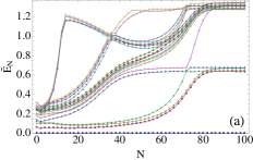
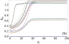
Figure 8: (color online) Scaled NRG eigenenergy flows with the iteration $N$ for a two-level QD coupled to normal leads (case II) with (a) $\gamma=0.5$ and $J/D=-0.9$ and (b) $\gamma=1$ and $J/D=-1.2$.

$$J_{4}\widetilde{S}_{\bar{q}}\cdot\widetilde{s}_{bb}.$$ (47)

The antiferromagnetic coupling will eventually screen out the remaining Kondo spin $\widetilde{S}_{\bar{q}}$ at a lower Kondo temperature $T_{K,2}$ since $J_{4}<J_{1}$. Hence the system undergoes two-stage Kondo effectsPustilnik01 as the temperature goes down: Two Kondo spins are screened out one by one since their couplings to relevant conduction-band degrees of freedom are different in magnitude. The ground state is of the spin singlet at low temperatures $(T<T_{K,2})$ due to complete screening, while the partial screening in the intermediate temperature $T_{K,2}<T<T_{K,1}$ leaves the system in the spin doublet. We have confirmed this scaling analysis numerically by examining the RG flow of the scaled low-lying eigenenergies in the NRG procedure. Figure 8 (a) clearly shows that the flow is in the high-temperature regime attracted by an unstable fixed point and then goes to the stable fixed point in the lower temperature.

The spin exchange coupling ${J_{\rm I}}\,\widetilde{\mathbf{S}}_{a}\cdot\widetilde{\mathbf{S}}_{b}$ can interrupt the Kondo correlation. In fact, we have observed that the two-stage Kondo effect ceases to happen if the exchange coupling ${J_{\rm I}}$ is so antiferromagnetic that ${J_{\rm I}}>k_{B}T_{K,1}$. In this regime, the Kondo spins are frozen to form a spin singlet by themselves before the conduction-band electrons screen them out. Hence, at zero temperature the system undergoes a transition between a Kondo state and an antiferromagnetic state as the exchange coupling ${J_{\rm I}}$ is varied. In contrast to the case I, however, the transition does not involve any change in the spin state: The ground state in both states is of the spin singlet. Note that the two-stage Kondo effect arises in the ferromagnetic side in the two-channel case while the one in the single-channel case happens in the antiferromagnetic side.

It may be interesting to consider a special case when the two Kondo temperatures are equal to each other: $T_{K,1}=T_{K,2}$. This can happen when $J_{a}=J_{b}$ so that $J_{1}=J_{4}=J_{a}+J_{ab}$, $J_{2}=J_{3}=J_{a}-J_{ab}$, and $J_{5}=0$, giving rise to the exchange Hamiltonian:

$$J_{1}\left(\widetilde{\mathbf{S}}_{q}\cdot\widetilde{\mathbf{s}}_{aa}+\widetilde{\mathbf{S}}_{\bar{q}}\cdot\widetilde{\mathbf{s}}_{bb}\right)+J_{2}\left(\widetilde{\mathbf{S}}_{q}\cdot\widetilde{\mathbf{s}}_{bb}+\widetilde{\mathbf{S}}_{\bar{q}}\cdot\widetilde{\mathbf{s}}_{aa}\right)$$ (48)

$$\mbox{}+{J_{\rm I}}\,\widetilde{\mathbf{S}}_{a}\cdot\widetilde{\mathbf{S}}_{b}.$$

Since $J_{1}>J_{2}$, the Kondo spins $\widetilde{\mathbf{S}}_{q}$ and $\widetilde{\mathbf{S}}_{\bar{q}}$ are simultaneously screened by the localized spins $\widetilde{\mathbf{s}}_{aa}$ and $\widetilde{\mathbf{s}}_{bb}$, respectively, defining a same Kondo temperature $T_{K}$. The RG flow in the NRG procedure confirms that there exist no unstable fixed point and that only one Kondo temperature governs the flow: see Fig. 8 (b). In our system, the condition $J_{a}=J_{b}$ is satisfied with $\gamma=1$ under the particle-hole symmetry condition.

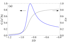
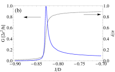
Figure 9: (color online) Phase shift and linear conductance as functions of $J$ for a two-level QD coupled to normal leads (case II) with $\gamma=1$ [(a)] and 0.5 [(b)].

The transport in the vicinity of the singlet-triplet transition of the isolated dot and on both of the antiferromagnetic and ferromagnetic sides can be analyzed by measuring the linear conductance from the NRG calculations. According to the Landauer-Büttiker formula in terms of the scattering matrix,Pustilnik01 the zero-temperature linear conductance can be expressed in terms of the phase shift $\delta_{s}$ for each channel:

$$G=\frac{2e^{2}}{h}\sin^{2}\delta,$$ (49)

with phase difference $\delta=\delta_{a}-\delta_{b}$. We have extracted the phase shifts from the energy spectrum in the NRG procedure by using the fact that the fixed point is described by a non-interacting Fermi liquid.Hofstetter04 On the ferromagnetic side, the Kondo screening forms a resonance level on each channel, which corresponds to a phase shift $\pi/2$ in both channels and $\delta=0$. On the antiferromagnetic side, on the other hand, both QD electrons occupy the orbital 1 so that $\delta_{a}=\delta_{1}=\pi$ and $\delta_{b}=0$, resulting in $\delta=\pi$. It implies that the conductance, Eq. (49) must approach zero on both sides of the singlet-triplet transition of the isolated dot while it has a maximum near the transition when $\delta=\pi/2$. Figure 9 shows that the phase difference increases rapidly from zero to $\pi$ near the transition point $(J\approx-0.8D)$ and that the conductance reaches the unitary limit when $\delta=\pi/2$. The maximal conductance point is shifted with respect to the bare singlet-triplet transition point $J=-0.8D$ since the dot-lead correlation favors the spin singlet state energetically [see Eq. (39b)]. As can be seen from Fig. 9, the zero-temperature linear conductance does not reflect the presence of two different Kondo scales: the qualitative feature of the conductance is same for $\gamma=1$ and $\gamma<1$. Inclusion of Zeeman splitting,Hofstetter04 finite temperatures, or superconductivity can, however, alter the low-temperature transport property dramatically if the relevant energy scale is between two Kondo temperatures and one of the Kondo correlation with lower Kondo temperature is suppressed. In the next section, we study how it happens in Josephson junctions.

IV.2 Superconducting Leads: $\Delta\neq 0$

Now we investigate the TLQD Josephson junction with $\Delta\neq 0$, considering the single- and two-channel cases separately as in the study of normal-lead case. The system state is identified as in the study of the weak-coupling regime: refer to Sec. III.1 for the definitions of labels of the system state and phase boundaries. Here we introduce a new label $D$ to denote the spin-doublet ground state which is missing in the weak-coupling regime.

A series of studies on the single-level QD Josephson junctionShiba69 ; Glazman89 ; Spivak91 ; Rozhkov99 ; Ryazanov01 ; Kontos02 ; Choi04 ; Siano04 ; Karrasch08 have already revealed that the competition between the Kondo effect and the superconductivity can lead to a Kondo-driven phase transition between the Kondo-dominant and superconductivity-dominant states and that the transition can be driven by tuning the relative strength between the Kondo temperature $T_{K}$ and the superconducting gap $\Delta$. Strong conductivity $(\Delta\gg T_{K})$ in the leads enforces the conduction electrons to form Copper pairs by themselves and does not interfere the spin correlation between the QD electrons. In the opposite limit ($\Delta\ll T_{K})$, however, the conduction-band electrons in the leads screen out the QD spins through spin-flip processes. Hence one can expect that as $\Delta$ is decreased the system undergoes a phase transition from states that prevail in the weak-coupling limit to other states governed by the Kondo effect. Below we find out that the superconducting gap introduces an infrared energy cutoff to the system and acts like a coherent probe for the Kondo excitation spectrum. Therefore, we expect that distinct Kondo effects in the two cases – cases I and II – should lead to different phase diagrams in the presence of the superconductivity even at zero temperature.

IV.2.1 Case I: Single Channel

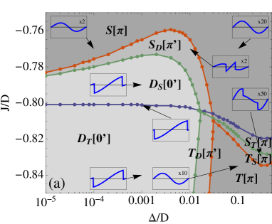
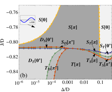
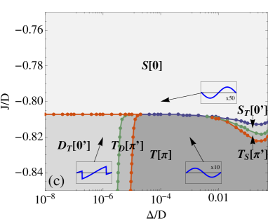
Figure 10: (color online) Phase diagrams in the $\Delta$-$J$ plane for the case I with $\gamma=1$ [(a)], 0.4 [(b)], and 0.1 [(c)]. The phase boundaries are located when the ground-state spin is changed at $\phi=0$ (red line), $\pi/2$ (green line), and $\pi$ (blue line). The yellow line separates two states with same ground-state spin but different SPRs. Refer the detailed classification of the states to the text. The insets show the SPRs for $\phi\in[-\pi,\pi]$ at the points indicated by the arrows. Here the solid lines are guide for eyes.

Weak Coupling Regime— Figure 10 shows the phase diagrams in the $\Delta$-$J$ plane in the case I. As expected, the NRG calculations confirm the results of the perturbation theory in the weak coupling limit ($\Delta/T_{K}\gg 1$). The system undergoes the singlet-triplet transition through intermediate states, $S_{T}$ and $T_{S}$, as $J$ is tuned. The phase boundaries between them are in perfect agreement with ones found from the perturbation theory: compare Figs. 3 and 10. Not only the superconductivity-induced renormalization of the singlet-triplet splitting is well reproduced, but also its asymptotic behavior ($\delta{J_{\rm I}}\to 0$) is correctly predicted in the limit $\Delta\to 0$ where the perturbation theory breaks down. Note that the normal-lead contribution to ${J_{\rm I}}$ [see Eq. (39b)] becomes effective for $\Delta\ll\Gamma$, leaving $\delta{J_{\rm I}}$ finite. The SPRs calculated from Eq. (35) also clearly follow those of the perturbative results: compare the insets of Figs. 3 and 10. At $\gamma=1$, the SPR is of the $\pi$-junction regardless of the spin of the ground state, while that of the spin singlet state becomes of the 0-junction as $\gamma$ is decreased.

Strong Coupling Regime— For smaller $\Delta$, on the other hand, the transition to the spin doublet state takes place, which is clearly ascribed to the Kondo effect. The conduction-band electrons in the effective single channel screen out one of the two QD spins, leaving the other unscreened. We have observed that the transition takes place at values of $\Delta\approx T_{K}$ [see red lines in Fig. 10], where $T_{K}$ is the Kondo temperature estimated from the width of the transmission coefficient in the normal-lead case [refer to Fig. 7 for $\gamma=1$]. The phase transition is highly dependent on the values of $J$ and exhibits asymmetric structure with respect to the sign of ${J_{\rm I}}$. On the ferromagnetic side $({J_{\rm I}}<J_{c})$ the system experiences a transition from the spin triplet to the spin doublet state with decreasing $\Delta$, while on the antiferromagnetic side $({J_{\rm I}}>J_{c})$ the singlet-doublet-singlet double transition is observed. In the strongly antiferromagnetic side (${J_{\rm I}}\gg J_{c}$) there exists no transition at all. This $J$-dependence of the transition originates from the fact that the spin exchange coupling affects the Kondo effect as discussed in Sec. IV.1.1. First, on the ferromagnetic side $({J_{\rm I}}<J_{c})$, the Kondo temperature decreases with increasing $|\Delta J|$. It explains the shift of the $T$-$D$ phase boundary in Fig. 10 toward smaller $\Delta$ with increasing $|J|$.Lee08 On the antiferromagnetic side $({J_{\rm I}}>J_{c})$, a two-stage Kondo effect with two Kondo temperature $T_{K}$ and $T_{K}^{I}$ takes place for small $\Delta J$. As long as $\Delta>T_{K}^{I}$, the second Kondo effect does not appear since the superconducting gap blocks any quasi-particle excitation within the gap $\Delta$. Therefore, for $T_{K}^{I}<\Delta<T_{K}$, one Kondo spin remains unscreened, forming the spin doublet state. For $\Delta\lesssim T_{K}^{I}$, however, Cooper pairs notice the suppression of the Kondo resonance level, and their tunneling is governed by cotunneling under strong Coulomb interaction, restoring the weak-coupling supercurrent in the presence of the spin singlet correlation. Hence the observed shape of the $S$-$D$ phase boundary and the reentrant behavior are well explained by the fact that the first Kondo temperature $T_{K}$ decreases with increasing $\Delta J$ as in the ferromagnetic side and that the second one $T_{K}^{I}$ decreases with decreasing $\Delta J$ and vanishes as $\Delta J\to 0$.

Finite Phase Difference— The transition boundaries depend on the phase difference $\phi$, which is responsible for the occurrence of the intermediate states. One should note that in the presence of finite $\Delta$ and $\phi$ both of two conduction-band channels are coupled to the QD: All the elements of the dot-lead coupling matrix, Eq. (27) become finite. In addition, the finite $\Delta$ makes it impossible to decouple one channel completely via any unitary transformation. However, the effect of the second channel is energetically cut off by the finite gap $\Delta$ itself in a sense that the Kondo temperature due to the coupling to the second channel is always smaller than $\Delta$. The single-channel argument is thus sufficient to account for the phase transitions even at finite $\phi$. The dot-lead coupling matrix, Eq. (27) then indicates that the couplings $t_{ab}$ and $t_{bb}$ responsible for the Kondo effect are reduced from $\sqrt{2}t$ to $\sqrt{2}t\cos\frac{\phi}{4}$, which accordingly lowers the Kondo temperature. The decrease of the Kondo temperature is clearly demonstrated in the phase diagrams: The phase boundaries at $\phi=\pi/2$ [see green lines in Fig. 10] are located at smaller $\Delta$ than those at $\phi=0$ and the regime of double transition is shrunken due to the increase of the second Kondo temperature $T_{K}^{I}$ [see Eq. (40)]. However, not only the diminished dot-lead coupling is responsible for the reduction of the Kondo temperature. We have found that a scaling analysis with finite $\Delta$ produces exotic terms (like proximity terms) which are missing in the normal-lead case. Such terms with finite $\phi$ can suppress the Kondo correlation further by twisting the phase correlation between two leads. We have observed that at the maximally twisted condition, that is, $\phi=\pi$, no Kondo state appears at all so that the Kondo state exists only in the intermediate state. Such a vulnerability of the Kondo effect at a maximally twisted phase condition to any finite magnetic perturbation was also observed in the magnetic molecular JJ.Lee08 The Kondo state may survive the maximally twisted condition only if there is no additional magnetic interaction $({J_{\rm I}}=0)$ as in the single-level QD-JJ. In our system, however, no appearance of the Kondo state at $\phi=\pi$ is observed even along the $D_{T}$-$D_{S}$ boundary where the effective splitting is supposed to vanish $(J\approx J_{c})$. We attribute it to the fact that the superconductivity shifts the energy levels of the QD spin states and induces the $\phi$-dependent singlet-triplet splitting, which seems to favor energetically the spin singlet or triplet states over the Kondo state.

SPR and Andreev Levels— Once the Kondo correlation prevails over the superconductivity, a resonant level is formed at the Fermi level, and the Cooper pairs tunnel through the Kondo resonant state, resulting in a ballistic 0-junction. Together with the $\phi$-dependent phase transition, the resonant tunneling makes the curve of the SPR break into three distinct segments as soon as the Kondo effect becomes effective, as seen in the insets of Fig. 10. The central segment resembles that of a ballistic short junctions, while the two surrounding segments are parts of the tunneling SPR for the spin singlet or triplet states. Since the Kondo state does not occur at $\phi=\pm\pi$, the SPR keeps the three-segment structure and does not become of the perfect ballistic junction that was observed in the single-level QD-JJ.Choi04

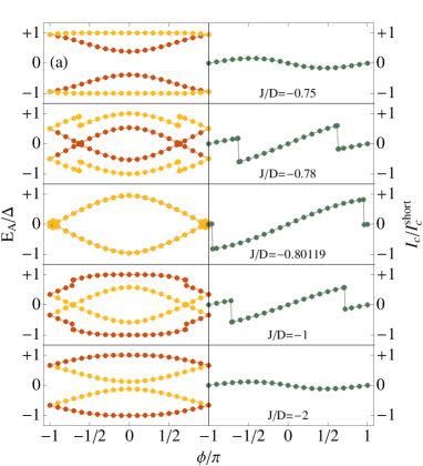
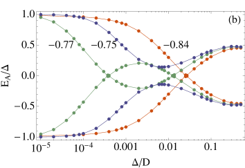
Figure 11: (color online) (a) (LEFT) Andreev levels in units of $\Delta$ and (RIGHT) supercurrent $I$ in units of $I_{c}^{\rm short}$ as functions of $\phi$ and $\Delta/D=10^{-3}$ for various values of $J$ as annotated. Red and yellow dots/lines denote the spin singlet and triplet Andreev levels, respectively. (b) Andreev levels (close to the Fermi level) in units of $\Delta$ as functions $\Delta/D$ at $\phi=0$ for several values of $J$ as labeled. Here we used $\gamma=1$.

Figure 11 (a) displays typical variations of the Andreev levels and supercurrent with $J$ at a fixed value of $\Delta/D=10^{-3}$. On the $D_{T}$-$D_{S}$ boundary with ${J_{\rm I}}\approx J_{c}$ [see the middle plots], the spin-singlet(red) and triplet(yellow) Andreev levels are degenerate in the central segment, while the degeneracy is lifted in side segments around $\phi=\pm\pi$. Any finite effective singlet-triplet splitting, ${J_{\rm I}}\neq J_{c}$, clearly induces a spin splitting in the subgap excitations, lifting the degeneracy, and consequently shifts the crossing between the ground state and the lowest excitation toward $\phi=0$, shrinking the central segment. Across the crossing, the ground-state spin is changed from 1/2 to 0 (1) for ${J_{\rm I}}>J_{c}$ $({J_{\rm I}}<J_{c})$. Similarly, the Andreev levels exhibit discontinuities in the spectra; for ${J_{\rm I}}>J_{c}$ $({J_{\rm I}}<J_{c})$, two outmost Andreev levels with spin 1 (0) in the central segment cannot remain as one-electron excitations with respect to the spin-0(1) ground state at the transition and are replaced by new Andreev levels with spin 1/2. In parallel with the abrupt change in the Andreev levels, the SPR shows a discontinuous sign change (note that $I\propto-\partial E_{a}/\partial\phi$, as the continuum-excitation contribution is negligible), culminating in a transition from the 0 to the $\pi$ state: accordingly, the states $D_{S}/D_{T}$ and $S_{D}/T_{D}$ are of the $0^{\prime}$ and $\pi^{\prime}$ states, respectively. As ${J_{\rm I}}$ grows in magnitude, the central segment shrinks and eventually vanishes. The SPR then becomes sinusoidal, which is that of a tunnel junction. Once the tunneling junction is fully established, stronger singlet-triplet splitting does not lead to any qualitative change in the SPR. The observed 0-$\pi$ transition is quite asymmetric with respect to the sign of ${J_{\rm I}}$. First, the phase transition in the antiferromagnetic region (${J_{\rm I}}>J_{c}$) takes place at ${J_{\rm I}}\lesssim T_{K}$, while the 0 state survives much larger ferromagnetic coupling (${J_{\rm I}}<J_{c}$). Second, the antiferromagnetic spin splitting gives rise to a double 0-$\pi$ transition that restores the spin singlet correlation at small $\Delta$. Figure 11 (b) clearly shows that for the antiferromagnetic ${J_{\rm I}}$ less than $T_{K}$ (at $J=-0.77$) the Andreev levels make double crossings as $\Delta$ is varied and the spin singlet ground state is restored at small $\Delta$. This is not the case in the ferromagnetic region (at $J=-0.84$) where only one crossing appears nor in the strongly antiferromagnetic region (at $J=-0.75$) where there exists no crossing at all. Note that the crossing takes place only when the spin-doublet ground state is replaced by the spin-singlet or triplet ones: No crossing appears in switching between the spin singlet and triplet ground states since each of them cannot be a single-particle excitation to the other.

Asymmetric Coupling— The phase diagram is also sensitive to the asymmetry factor $\gamma$ as well. The decrease of $\gamma$ gives rise to the shrink of the intermediate states $S_{D}$ and $D_{S}$ in the antiferromagnetic side and the shift of the $T$-$T_{D}$ and $T_{D}$-$D_{T}$ boundaries toward smaller values of $\Delta$ [compare the phase diagrams in Fig. 10]. To understand this behavior, one should take a look at the typical dependence of the Kondo temperature $T_{K}$ on the lead-dot coupling: $T_{K}\propto\exp\left[-A/\Gamma_{\rm tot}\right]$, where $\Gamma_{\rm tot}=2(1+\gamma^{2})\Gamma$ is the total hybridization and $A$ is a $\Gamma$-independent constant. As $\gamma$ is decreased from 1 to 0, the total hybridization decreases from $4\Gamma$ to $2\Gamma$, which leads to the exponential decrease of the Kondo temperature. Hence, with the smaller $T_{K}$, the transitions from the spin double state to the spin singlet or triplet states occur at smaller values of ${J_{\rm I}}$ or $\Delta$. The exponential dependence of $T_{K}$ and $T_{K}^{I}$ on $\gamma$ makes the intermediate states $S_{D}$ and $D_{S}$ almost vanish and hard to detect even at $\gamma\approx 0.4$.

Another effect of the asymmetry is the appearance of a second 0 state in the singlet side in small-$\Delta$ region [see Fig. 10 (b)]. This 0 state is not like the one predicted from the perturbation theory which works only in the large-$\Delta$ limit. In the small-$\Delta$ limit, all the high-order processes should be taken into account in order to determine the sign of the supercurrent. Even though the analytical analysis taking all the orders of the processes is difficult to apply, a rough account can be proposed: From the lowest-order terms, Eqs. (77) and (78), one can know that the sign of the supercurrent due to each tunneling process is determined based on which intermediate two-electron state appears in the middle of the tunneling process. For example, processes with an intermediate spin singlet state $\left|2,0,0;3\right\rangle$ make a positive contribution. In higher-order processes, different kinds of intermediate states will appear one by one, and a negative contribution can arise only for processes with an odd number of the intermediate states that invert the sign of the current. Since processes with an even number of sign-inverting states should outnumber odd-number processes, one can claim that higher-order processes are likely to make the positive contribution and consequently to favor the 0 state. We observe that this 0 state takes place for $\gamma<1$ and that at $\gamma=1$ the spin singlet state is purely the $\pi$ state. We guess that the second 0 state also benefits from the weakening of the negative $\beta^{\prime}_{S5}$ term with decreasing $\gamma$. Figure 10 (b) shows that the second 0 state expands toward large-$\Delta$ region as $J$ is increased. It can be explained by the argument that with increasing $J$ the positively contributing processes with the intermediate state $\left|2,0,0;3\right\rangle$ have larger amplitude because the energy cost $E_{0;3}-E_{0;1}=\delta\epsilon-3J/4$ diminishes; see Eq. (78). At smaller $\gamma$, the two 0 states expand further and eventually merge to form a single 0 state, as shown in Fig. 10 (c).

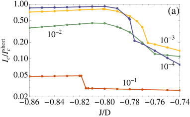
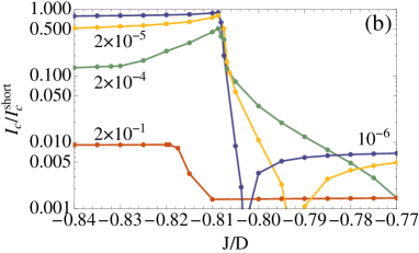
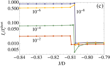
Figure 12: (color online) Critical currents as functions of $J/D$ in units of $I_{c}^{\rm short}$ for the case I with $\gamma=1$ [(a)], 0.4 [(b)], and 0.1 [(c)]. The numbers next to the lines represent the values of $\Delta/D$ chosen for them. Here the solid lines are guide for eyes.

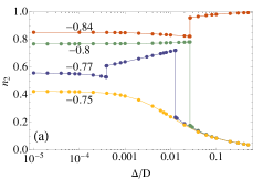
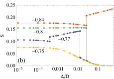
Figure 13: (color online) (a) Occupation $\left\langle n_{2}\right\rangle$ in the second level of the QD and (b) spin correlation $\left\langle{\mathbf{S}}_{1}\cdot{\mathbf{S}}_{2}\right\rangle$ as functions of $\Delta/D$ for the case I at $\gamma=1$ and $\phi=0$. The numbers next to the lines represent the values of $J/D$ chosen for them. Due to the particle-hole symmetry, we have $\left\langle n_{1}\right\rangle=2-\left\langle n_{2}\right\rangle$. Here the solid lines are guide for eyes.

Critical Current— Figure 12 shows the critical current as a function of $J/D$ for given values of $\Delta$. For all values of $\gamma$, the spin triplet state has a larger critical current than the spin singlet state, which is consistent with the perturbation results: compare Figs. 4 and 12. The critical current is considerably boosted up in the Kondo-dominant state and even approaches the ballistic short-junction value $I_{c}^{\rm short}$ as it goes deep into the Kondo state. The critical current has its maximum around the singlet-triplet transition point and decreases rapidly in the antiferromagnetic side. A dip in the critical current is observed in the antiferromagnetic side at moderate values of $\gamma$. This dip happens at the boundary between the $\pi$ state and the second 0 state where the current vanishes completely. Note that the Kondo-driven 0-$\pi$ transition involves intermediate states so that the current does not vanish at the phase boundaries.

Occupation and Spin Correlation— Finally, we’d like to mention about the other ground-state properties such as the QD occupation and the spin correlation between QD spins. For the isolated QD, the perfect spin singlet state dictates $\left\langle n_{1}\right\rangle=2$, $\left\langle n_{2}\right\rangle=0$, and $\left\langle{\mathbf{S}}_{1}\cdot{\mathbf{S}}_{2}\right\rangle=0$, while $\left\langle n_{1}\right\rangle=1$, $\left\langle n_{2}\right\rangle=1$, and $\left\langle{\mathbf{S}}_{1}\cdot{\mathbf{S}}_{2}\right\rangle=1/4$ in the spin triplet state. This behavior is well reproduced for large values of $\Delta$ [see Fig. 13]. The strong superconductivity effectively decouples the QD from the leads, and the correlations between QD spins are left unpolluted. As $\Delta$ is decreased, on the other hand, the dot-lead hybridization interferes the QD spin correlation and makes $\left\langle n_{i}\right\rangle$ and $\left\langle{\mathbf{S}}_{1}\cdot{\mathbf{S}}_{2}\right\rangle$ deviate from their bare values. Furthermore, they exhibit abrupt changes at phase transitions to the spin doublet state; $\left\langle n_{2}\right\rangle$ and $\left\langle{\mathbf{S}}_{1}\cdot{\mathbf{S}}_{2}\right\rangle$ exhibit the same qualitative dependence on $\Delta$ since the occupation in the orbital 2 is directly related to the formation of the spin triplet state. Interestingly, the emergence of the Kondo spin correlation which screens out one of the spins does not completely suppress the local spin correlation between QD spins and even help its recovery slightly as $\Delta$ is further decreased.

IV.2.2 Case II: Two Channels

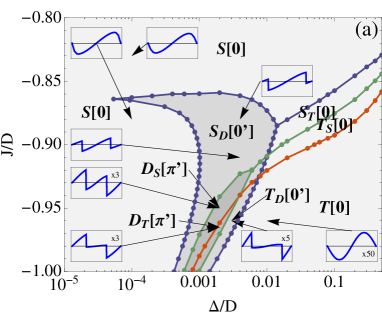
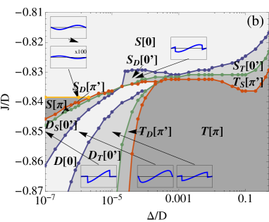
Figure 14: (color online) Phase diagrams in the $\Delta$-$J$ plane for the case II with $\gamma=1$ [(a)] and 0.5 [(b)]. Refer to Fig. 10 for the details.

Weak Coupling Regime— Now we consider the two-channel case in the presence of the superconductivity. Figure 14 displays the phase diagrams in this case. In the large-$\Delta$ limit the phase boundaries and the SPR characteristics coincide well with those obtained from the perturbative theory: compare Figs. 5 and 14. At $\gamma=1$, the SPR is of the 0-junction in both the spin singlet and triplet states, and that of the state $T$ switches into the $\pi$-junction as $\gamma$ is decreased.

Strong Coupling Regime— The small-$\Delta$ part of the phase diagram, on the other hand, features Kondo-oriented structures. First, consider the asymmetric case ($\gamma\neq 1$) [see Fig. 14 (b)] which exhibits typical phase diagram in two-channel case. On the antiferromagnetic side no transition is observed to take place. In this regime the antiferromagnetic coupling is strong enough that the system is frozen in the spin singlet state regardless of value of $\Delta$. On the ferromagnetic side, however, the system experiences a double transition with decreasing $\Delta$: a transition from the spin triplet to the spin doublet state is followed by a second transition to the spin singlet state at smaller $\Delta$. It reflects the two-stage Kondo effect discussed in Sec. IV.1.2, where two Kondo scales $T_{K,1}$ and $T_{K,2}$ are operating. For $\Delta>T_{K,1/2}$, the conduction-band electrons form the Cooper pairs by themselves without affecting the ferromagnetic correlation formed in the QD. Once $\Delta$ is lowered below the larger Kondo temperature $T_{K,1}$ so that $T_{K,2}<\Delta<T_{K,1}$, one of the QD spins is screened out and the other spin that is left unscreened defines the spin doublet state. For smaller $\Delta<T_{K,1/2}$, the remaining QD spin is also screened out so that the entire system becomes of the spin singlet. We have spotted such a double transition at any value of $\phi$. Figure 14 (b) shows that the phase difference affects the Kondo temperatures in such a way that $T_{K,1}$ ($T_{K,2}$) decreases (increases) with increasing $\phi$. The interval $T_{K,1}-T_{K,2}$ is the smallest at $\phi=\pi$. As in the case I, the modulation of the Kondo temperatures can be roughly understood from the dependence of the dot-lead coupling on $\phi$ [see Eq. (27)]: The phase difference redistributes the amplitude of dot-lead couplings so that the stronger one get weaker and vice versa as $\phi$ is varied from 0 to $\pi$. As a result, with decreasing $\Delta$ the system evolves from the spin triplet state $T$ to the singlet state $S$ via all the possible intermediate states including the complete spin doublet state $D$.

Symmetric Case— In the symmetric case ($\gamma=1$), however, the phase diagram exhibits quite different features [see Fig. 14 (a)]. At $\phi=0$ only one direct transition from the spin triplet to the spin singlet is observed [see a red line]. It is surely due to the disappearance of the two-stage Kondo effect at $\gamma=1$: two QD spins are simultaneously screened at a common Kondo temperature $T_{K}$ [refer to Sec. IV.1.2]. Hence the system passes from the spin triplet state to the spin singlet state either by antiferromagnetic coupling or by Kondo correlation. At finite $\phi$, however, the redistribution of the dot-lead couplings deviate the Kondo couplings for two QD spins from their symmetric point so that one becomes larger and the other smaller, recovering the two-stage Kondo effect with two Kondo temperatures $T_{K,1}>T_{K,2}$ again. In this case $T_{K,1}$ ($T_{K,2}$) increases (decreases) with $\phi$ so that the interval $T_{K,1}-T_{K,2}$ reaches its maximum at $\phi=\pi$. As a result no complete $D$ state arises as the spin triplet state is changed into the spin singlet state.

One more peculiarity in the symmetric case is a cusp in the phase boundary at $\phi=\pi$ [see Fig. 14 (a)]. Note that such a strange structure is also observed in the asymmetric case [see Fig. 14 (b)]. Analytical theory to capture its physical origin is not available because the perturbative scaling theory with finite $\Delta$ is hard to trace down. Instead, we draw a tentative argument from its structural resemblance to that caused by the single-channel two-stage Kondo effect. Our NRG calculation indicates that at $\phi=\pi$ the lower Kondo temperature $T_{K,2}$ in the ferromagnetic side exponentially decreases as $J$ approaches the antiferromagnetic region. As soon as the effective singlet-triplet splitting ${J_{\rm I}}$ becomes antiferromagnetic, the spin exchange coupling ${J_{\rm I}}\widetilde{\mathbf{S}}_{a}\cdot\widetilde{\mathbf{S}}_{b}$ can then cause the second Kondo effect with the Kondo temperature $T_{K}^{I}$ between the spin ${\mathbf{S}}_{\bar{q}}$ and the local Fermi liquid formed at the spin ${\mathbf{S}}_{q}$ as explained in Sec. IV.1.1. Accordingly, we have again a two-stage Kondo effect that explains the upward convex shape of the unusual phase boundaries very well. The condition that it can take place is that $T_{K,2}<T_{K}^{I}$, that is, the second QD spin is screened by the continuous degrees of freedom formed at the Kondo resonance level at the first QD spin rather than by the conduction-band electrons in leads. In the absence of superconductivity this does not arise because $T_{K,2}$ is always larger than $T_{K}^{I}$. However, the NRG calculation suggests that this condition is satisfied with finite $\Delta$ and more importantly with $\phi\approx\pi$.

SPR for the Asymmetric Case— The SPRs shown in the insets of Fig. 14 clearly reflects the Kondo-driven phase transition. The asymmetric case [see Fig. 14 (b)] displays the similar evolution of the SPR with respect to the alteration of the ground-state spin as observed in the single-channel case. The formation of the Kondo-assisted resonant level boosts up the tunneling of Cooper pairs and develops the ballistic 0-junction. Starting from the tunneling $\pi$-junction in the spin triplet state, the SPR then has a shape of the three-segment structure with decreasing $\Delta$. The central ballistic part enlarges further with lowering $\Delta$, and the SPR becomes of the complete 0-junction as the system enters into the state $D$. Passing through the second transition to the spin singlet state, the SPR restores the three-segment form and eventually returns to the $\pi$-junction. It is worth noting that while the ballistic 0-junction is ascribed to the Kondo resonant tunneling, its suppression at smaller $\Delta$ is also due to the Kondo effect. The destructive interference between two resonant tunnelings leads to a subduing of the tunneling current. The interference is not complete (while it is the case in the single-channel case) and becomes ineffective as $J$ becomes less negative, resulting in an increase of the supercurrent.

The phase diagram in Fig. 14 (b) shows that there exist two spin singlet states $S$ with 0- and $\pi$-junctions, respectively. The perturbative analysis manifests that the spin singlet state in the case II pertains to the 0-junction behavior. Our NRG calculation shows that it is the case even in the small $\Delta$ limit as long as the antiferromagnetic coupling prevails. However, we found that in the Kondo-dominant singlet state the SPR exhibits the tunneling $\pi$-junction behavior as shown in Fig. 14 (b), following the SPR of the spin triplet state in the large-$\Delta$ regime. The transition between two singlet state does not involve any intermediate state so that the supercurrent completely vanishes at the boundary (yellow line) between them.

SPR for the Symmetric Case— The symmetric case, on the other hand, displays exotic features in the SPR as well as in the phase diagram. The most intriguing observation is that the Kondo-assisted tunneling triggers the ballistic $\pi$-junction behavior. As stated before, the Kondo-driven spin doublet state does not form at $\phi=0$ but comes into being from $\phi=\pi$ as $\Delta$ is decreased. The tunneling 0-junction SPR in the spin triplet state then transforms into the three-segment one that, at this time, has the Kondo-driven ballistic feature at its side segments, not in the central part. In addition, the SPR in the side segments exhibits the $\pi$-junction behavior: As observed in Fig. 11, the change of the ground-state spin from 1 to 1/2 makes the Andreev levels cross at the Fermi level, which accordingly induces sign change of the supercurrent across the crossing point. This ballistic $\pi$-junction can develop only if the dot-lead couplings are all comparable and their product is negative because only this condition ensures that the spin triplet state has the 0-junction and the Kondo transition starts at $\phi=\pi$ with $T_{K,1}(\phi=\pi)>T_{K,1}(\phi=0)$. The Kondo-assisted $\pi$-junction does not reach its full strength, through, and further lowering of $\Delta$ shrinks the side segments, finally restoring the 0-junction. Hence, in the small-$\Delta$ limit, the system is of the spin singlet in the 0 state.

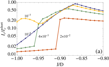
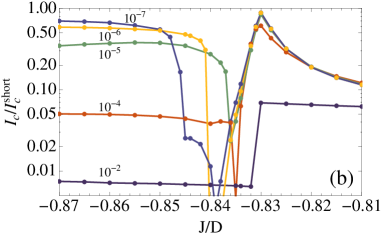
Figure 15: (color online) Critical currents as functions of $J/D$ in units of $I_{c}^{\rm short}$ for the case II with $\gamma=1$ [(a)] and 0.5 [(b)]. The numbers next to the lines represent the values of $\Delta/D$ chosen for them. Here the solid lines are guide for eyes.

Critical Current— Figure 15 shows the critical current as a function of $J/D$ for given values of $\Delta$. In the large-$\Delta$ limit, the critical current is larger in the spin singlet state than in the spin triplet state as predicted in the perturbation theory. On the other hand, the small-$\Delta$ critical current is observed to follow the linear conductance obtained in the normal-lead case: compare Figs. 9 and 15. The critical current exhibits a peak exactly where the linear conductance reaches its maximum. The peak is not due to the Kondo boosting but originates from the competition between the Kondo and the antiferromagnetic correlations at the singlet-triplet transition as revealed in Sec. IV.1.2. However, the Kondo boosting enhances the critical current in the spin doublet state. At a given $\Delta$, the system can be driven into the spin doublet state as $J$ is decreased, where the unscreened Kondo correlation opens a resonance tunneling. Hence, as can be seen in Fig. 15 (b), the small-$\Delta$ critical current features a peak and plateau as $J$ is varied. A sharp dip is also identified between them. The Kondo-assisted plateau is rather weak in the symmetric case [see Fig. 15 (a)] and it disappears in the small $\Delta$ limit since no spin doublet state exists in this limit [see Fig. 14 (a)]. Together with the Kondo-assisted $\pi$-junction, this double-peak or peak-plateau structure of critical current with respect to the spin exchange coupling $J$ contrast the two-channel case with the single-channel one, so it provides a way to distinguish two cases in experiments in which the amplitudes of dot-lead couplings are not known in priori.

V Discussion and Conclusion

We have investigated the physical properties and the electronic transport of two-level quantum dot Josephson junctions by focusing on two representative dot-lead coupling configurations, cases I and II [see Eq. (10)]. The fourth-order perturbation theory applied in the weak coupling limit has revealed that the parities of dot orbital wavefunctions, that is, the sign of the product of dot-lead tunneling amplitudes, can greatly affect the sign of the supercurrent depending on the spin correlation present in the dot. The key elements that determine the current characteristics are found to be the existence of a localized moment in orbitals which reverses the order of electrons in Cooper pairs and the competition between diagonal and offdiagonal tunneling processes.

In the strong coupling limit the Kondo correlation competes with the superconductivity and the spin exchange coupling and the system state is determined by their relative strength. We have used the NRG method and the scaling theory based on the Schrieffer-Wolff transformed Hamiltonian in order to examine the Kondo effect in the normal-lead counterpart of our system. The effective single-channel case (case I) exhibits three different states – underscreened $S=1$ Kondo effect, two-stage Kondo effect, and spin singlet state – depending on the sign and strength of the spin exchange coupling, while in the two-channel case (case II), the system displays two-stage Kondo effect and spin singlet state. We have found that the numerical results from the NRG method applied to superconducting case can be understood in terms of comparison between the superconducting gap $\Delta$ and relevant Kondo temperatures: The Kondo correlation found in the normal-lead case becomes effective once $\Delta$ becomes smaller than the corresponding Kondo temperature. In this way the superconducting gap acts like a coherent energy probe for the excitations of the system otherwise. The competition between the superconductivity and the many-body correlations present in the system gives rise to phase transitions which accompany abrupt changes in physical properties such as ground-state spin and SPR: Among the prominent changes that arise once the Kondo effect prevails over superconductivity are the boost-up of the supercurrent due to resonant tunneling and the appearance of strong 0-junction. Knowing the magnitude of the superconducting gap that is under control, therefore, it provides a way to measure the magnitude of the important many-body correlations such as the Kondo temperature or vice versa.

Beside detecting the system excitations, the superconductivity directly alters the system state. In the weak coupling limit it renormalizes the singlet-triplet splitting and shifts the singlet-triplet transition point which now depends on the phase difference as well. In the strong coupling limit the finite phase difference influences the interference mechanism and suppress or enhance the other many-body effects. Especially, at the maximally twisted condition ($\phi=\pi$), the Kondo correlation is completely suppressed in the case I and the Kondo-assisted $\pi$-junction is induced in the case II. Knowing that the $\pi$-junction in most of cases is usually weak due to its perturbative origin, the latter mechanism opens a way to have a strong $\pi$-junction. In the light of quantum computational unit which is free of any magnetic control, this $\pi$-junction is more promising because the state of the junction can be controlled by electric manipulation: the spin exchange coupling can be tuned by the gate voltage.

We expect that our theoretical prediction about phase diagrams and SPRs in TLQD-JJs can be explored in experiment by using state-of-art fabrication techniques. A recent experimentRoch08 measured electronic transport through C₆₀-molecular junctions and detected the singlet-triplet transition and the accompanying Kondo effects which are consistent with existing theories. The same experiment group has extended their study to superconducting caseWinkelmann09 where the Al bars are attached on top of Au leads coupled to C₆₀ and the superconductivity is induced in Au leads by the proximity effect. The Josephson effect predicted in our paper can be then investigated by forming a SQUID,Cleuziou06 one of which arms contains the molecular junction. As implemented in Roch et al.,Roch08 the spin exchange coupling can be then controlled by an externally applied gate voltage. Or, the superconducting gap can be tuned by applying a magnetic field as long as it does not suppress the Kondo effect. In this way the switching between 0 and $\pi$ states with respect to the tuning of $J$ and/or $\Delta$ predicted in our calculations could be confirmed in experiment. Even without using the SQUID geometry, our theory could be tested by measuring a critical current through the junction, which should exhibit nontrivial dependence on the spin exchange coupling as discussed above.

Appendix A Energy Shift Coefficients in Perturbation Theory

Here we present the detailed expressions of the coefficients $\beta_{ai}$ for $a=S,T$ are defined in the energy shifts, Eq. (11) in the fourth-order perturbation theory. On behalf of readability, we introduce the following integrals:

$$A_{i} \equiv\int\frac{dx/\pi}{f(x;\xi_{1i})}$$ (50)

$$A^{\prime}_{i} \equiv\int\frac{dx/\pi}{f(x;\xi_{1i})f(x)}$$ (51)

$$A_{ij} \equiv\int\frac{dx/\pi}{f(x;\xi_{1i})f(x;\xi_{1j})}$$ (52)

$$A_{ij}(\xi) \equiv\int\int\frac{dxdy/\pi^{2}}{f(x,y;\xi)f(x;\xi_{1i})f(x;\xi_{1j})}$$ (53)

$$A^{\prime}_{ij}(\xi) \equiv\int\int\frac{dxdy/\pi^{2}}{f(x,y;\xi)f(x)f(y)f(x;\xi_{1i})f(x;\xi_{1j})}$$ (54)

$$B_{ij}(\xi) \equiv\int\int\frac{dxdy/\pi^{2}}{f(x,y;\xi)f(x;\xi_{1i})f(y;\xi_{1j})}$$ (55)

$$B^{\prime}_{ij}(\xi) \equiv\int\int\frac{dxdy/\pi^{2}}{f(x,y;\xi)f(x)f(y)f(x;\xi_{1i})f(y;\xi_{1j})},$$ (56)

where we have defined $f(x)\equiv\sqrt{1+x^{2}}$, $f(x;\xi)\equiv f(x)+\xi$, and $f(x,y;\xi)\equiv f(x)+f(y)+\xi$ and all the integration should be done over the region $[-D/\Delta,D/\Delta]$. All the charge excitation energies that appear in the expressions are made dimensionless:

$$\xi_{11} =(\epsilon_{1}-E_{a}^{(0)})/\Delta, \xi_{12} =(\epsilon_{2}-E_{a}^{(0)})/\Delta,$$ (57)

$$\xi_{21} =-E_{a}^{(0)}/\Delta, \xi_{22} =(E_{0;1}-E_{a}^{(0)})/\Delta,$$ (58)

$$\xi_{23} =(E_{0;2}-E_{a}^{(0)})/\Delta, \xi_{24} =(E_{0;3}-E_{a}^{(0)})/\Delta,$$ (59)

$$\xi_{25} =(E_{1}-E_{a}^{(0)})/\Delta,$$ (60)

for $a={S,T}$, respectively. In terms of the integral macros, the coefficients $\beta_{Si}$ for the singlet energy shift are then expressed as

$$\beta_{S0} =-A_{1}$$ (61)

$$\beta_{S1} =A_{1}A_{11}-\frac{[A^{\prime}_{1}]^{2}}{\xi_{21}}$$ (62)

$$\quad\mbox{}-\frac{A_{11}(\xi_{21})+B_{11}(\xi_{21})}{2}-\frac{A_{11}(\xi_{22})+B^{\prime}_{11}(\xi_{22})}{2}$$

$$\beta_{S2} =2A_{1}A_{11}+A^{\prime}_{11}(\xi_{22})+B_{11}(\xi_{22})$$ (63)

$$\quad\mbox{}-\frac{A_{11}(\xi_{24})+B_{11}(\xi_{24})+A^{\prime}_{11}(\xi_{24})+B^{\prime}_{11}(\xi_{24})}{2}$$

$$\quad\mbox{}-\frac{5(A_{11}(\xi_{25})+B_{11}(\xi_{25})-A^{\prime}_{11}(\xi_{25})-B^{\prime}_{11}(\xi_{25}))}{2}$$

$$\beta_{S3} =2A_{1}A_{11}-\frac{A_{11}(\xi_{24})+B_{11}(\xi_{24})}{2}$$ (64)

$$\quad\mbox{}-\frac{3(A_{11}(\xi_{25})+B_{11}(\xi_{25}))}{2}$$

$$\beta_{S4} =2A_{1}A_{11}-A_{11}(\xi_{21})-B_{11}(\xi_{21})-A_{11}(\xi_{22})$$ (65)

$$\beta_{S5} =2B_{11}(\xi_{22})$$ (66)

$$\beta^{\prime}_{S4} =B^{\prime}_{11}(\xi_{22})+2\frac{[A^{\prime}_{1}]^{2}}{\xi_{21}}$$ (67)

$$\beta^{\prime}_{S5} =-2A^{\prime}_{11}(\xi_{22})+A^{\prime}_{11}(\xi_{24})+B^{\prime}_{11}(\xi_{24})$$ (68)

$$\quad\mbox{}-3(A^{\prime}_{11}(\xi_{25})+B^{\prime}_{11}(\xi_{25})),$$

where the scaled excitation energies are calculated with $E_{a}=E_{S}$. The coefficients $\beta_{Ti}$ for the triplet energy shift are given by

$$\beta_{T0} =-\frac{A_{1}+A_{2}}{2}$$ (69)

$$\beta_{T1} =\frac{(A_{1}+A_{2})(A_{11}+A_{22})}{4}$$ (70)

$$\quad\mbox{}-\frac{A_{11}(\xi_{24})+A_{22}(\xi_{24})+2B_{12}(\xi_{24})}{4}+\frac{A^{\prime}_{12}(\xi_{24})}{2}$$

$$\quad\mbox{}+\frac{B^{\prime}_{11}(\xi_{24})+B^{\prime}_{22}(\xi_{24})}{4}$$

$$\quad\mbox{}-\frac{A_{11}(\xi_{25})+A_{22}(\xi_{25})+B_{12}(\xi_{25})}{2}+A^{\prime}_{12}(\xi_{25})$$

$$\quad\mbox{}+\frac{B^{\prime}_{11}(\xi_{25})+B^{\prime}_{22}(\xi_{25})}{4}$$

$$\beta_{T2} =\frac{(A_{1}+A_{2})(A_{11}+A_{22})}{2}$$ (71)

$$\quad\mbox{}-A_{11}(\xi_{21})+B_{11}(\xi_{21})-A_{22}(\xi_{21})+B_{22}(\xi_{21})$$

$$\quad\mbox{}+2(A_{12}(\xi_{21})-B_{12}(\xi_{21}))$$

$$\quad\mbox{}-A_{11}(\xi_{22})-B_{11}(\xi_{22})+A^{\prime}_{11}(\xi_{22})+B^{\prime}_{11}(\xi_{22})$$

$$\quad\mbox{}-A_{22}(\xi_{23})+B_{22}(\xi_{23})+A^{\prime}_{22}(\xi_{23})+B^{\prime}_{22}(\xi_{23})$$

$$\quad\mbox{}+A_{12}(\xi_{24})-B^{\prime}_{12}(\xi_{24})$$

$$\quad\mbox{}+\frac{B_{11}(\xi_{24})+B_{22}(\xi_{24})-A^{\prime}_{11}(\xi_{24})-A^{\prime}_{22}(\xi_{24})}{2}$$

$$\quad\mbox{}-2A_{12}(\xi_{25})+A^{\prime}_{11}(\xi_{25})+A^{\prime}_{22}(\xi_{25})+B^{\prime}_{12}(\xi_{25})$$

$$\quad\mbox{}-\frac{B_{11}(\xi_{25})+B_{22}(\xi_{25})}{2}$$

$$\beta_{T3} =\frac{(A_{1}+A_{2})(A_{11}+A_{22})}{2}$$ (72)

$$\quad\mbox{}-\frac{A_{11}(\xi_{21})+A_{22}(\xi_{21})}{2}-B_{12}(\xi_{21})$$

$$\quad\mbox{}-\frac{A_{11}(\xi_{22})+B_{11}(\xi_{22})+A_{22}(\xi_{23})+B_{22}(\xi_{23})}{2}$$

$$\beta_{T4} =\frac{(A_{1}+A_{2})(A_{11}+A_{22})}{2}$$ (73)

$$\quad\mbox{}-\frac{A_{11}(\xi_{24})+A_{22}(\xi_{24})+2B_{12}(\xi_{24})}{4}$$

$$\quad\mbox{}-\frac{3A_{11}(\xi_{25})+3A_{22}(\xi_{25})+2B_{12}(\xi_{25})}{4}$$

$$\beta_{T5} =2A_{12}(\xi_{21})+B_{11}(\xi_{21})+B_{22}(\xi_{21})$$ (74)

$$\quad\mbox{}+A_{12}(\xi_{24})+\frac{B_{11}(\xi_{24})+B_{22}(\xi_{24})}{2}$$

$$\quad\mbox{}-3A_{12}(\xi_{25})-\frac{B_{11}(\xi_{25})+B_{22}(\xi_{25})}{2}$$

$$\beta^{\prime}_{T4} =-\frac{A^{\prime}_{12}(\xi_{24})}{2}-\frac{B^{\prime}_{11}(\xi_{24})+B^{\prime}_{22}(\xi_{24})}{4}$$ (75)

$$\quad\mbox{}-\frac{3A^{\prime}_{12}(\xi_{25})}{2}-\frac{B^{\prime}_{11}(\xi_{25})+B^{\prime}_{22}(\xi_{25})}{4}$$

$$\beta^{\prime}_{T5} =-A^{\prime}_{11}(\xi_{22})-B^{\prime}_{11}(\xi_{22})-A^{\prime}_{22}(\xi_{23})-B^{\prime}_{22}(\xi_{23})$$ (76)

$$\quad\mbox{}+\frac{A^{\prime}_{11}(\xi_{24})+A^{\prime}_{22}(\xi_{24})}{2}+B^{\prime}_{12}(\xi_{24})$$

$$\quad\mbox{}-\frac{3(A^{\prime}_{11}(\xi_{25})+A^{\prime}_{22}(\xi_{25}))}{2}-B^{\prime}_{12}(\xi_{25}),$$

where the scaled excitation energies are calculated with $E_{a}=E_{T}$. For better estimation of the sign and the magnitude of the supercurrent, full expressions for $\beta^{\prime}_{S4/5}$ and $\beta^{\prime}_{T4/5}$ are given below:

$$\beta^{\prime}_{S4} =\int\int\frac{dxdy/\pi^{2}}{f(x,y;\xi_{22})f(x;\xi_{11})f(y;\xi_{11})f(x)f(y)}+\frac{2}{\xi_{21}}\left(\int\frac{dx/\pi}{f(x;\xi_{11})f(x)}\right)^{2}$$ (77)

$$\beta^{\prime}_{S5} =\int\int\frac{dxdy/\pi^{2}}{f(x)f(y)}\Bigg{[}\left(\frac{1/2}{f(x,y;\xi_{24})}-\frac{3/2}{f(x,y,;\xi_{25})}\right)\left(\frac{1}{f(x;\xi_{11})}+\frac{1}{f(y;\xi_{11})}\right)^{2}-\frac{2}{f(x,y;\xi_{22})[f(x;\xi_{11})]^{2}}\Bigg{]}$$ (78)

$$\beta^{\prime}_{T4} =-\frac{1}{4}\int\int\frac{dxdy/\pi^{2}}{f(x)f(y)}\Bigg{[}\left(\frac{1}{f(x,y;\xi_{24})}+\frac{1}{f(x,y;\xi_{25})}\right)\left(\frac{1}{f(x;\xi_{11})f(y;\xi_{11})}+\frac{1}{f(x;\xi_{12})f(y;\xi_{12})}\right)$$ (79)

$$\quad\qquad\qquad\qquad\qquad\qquad\mbox{}+\left(\frac{1}{f(x,y;\xi_{24})}+\frac{3}{f(x,y;\xi_{25})}\right)\frac{2}{f(x;\xi_{11})f(x;\xi_{12})}\Bigg{]}$$

$$\beta^{\prime}_{T5} =-\frac{1}{2}\int\int\frac{dxdy/\pi^{2}}{f(x)f(y)}\Bigg{[}\frac{1}{f(x,y;\xi_{22})}\left(\frac{1}{f(x;\xi_{11})}+\frac{1}{f(y;\xi_{11})}\right)^{2}+\frac{1}{f(x,y;\xi_{23})}\left(\frac{1}{f(x;\xi_{12})}+\frac{1}{f(y;\xi_{12})}\right)^{2}$$ (80)

$$\qquad\mbox{}-\frac{1}{f(x,y;\xi_{24})}\left(\frac{1}{f(x;\xi_{11})}+\frac{1}{f(y;\xi_{12})}\right)^{2}+\frac{1}{f(x,y;\xi_{25})}\left(\frac{3}{[f(x;\xi_{11})]^{2}}+\frac{2}{f(x;\xi_{11})f(y;\xi_{12})}+\frac{3}{[f(y;\xi_{12})]^{2}}\right)\Bigg{]}.$$

References

- (1) B. D. Josephson, Phys. Lett. 1, 251 (1962); Rev. Mod. Phys. 46, 251 (1974).
- (2) M. Tinkham, Introduction to Superconductivity (McGraw-Hill, Singapore, 1996).
- (3) J. Bardeen, L. N. Cooper, and J. R. Schrieffer, Phys. Rev. 106, 162 (1957); 108, 1175 (1957).
- (4) H. Shiba and T. Soda, Prog. Theor. Phys. 41, 25 (1969).
- (5) L. I. Glazman and K. A. Matveev, Pis’ma Zh. Teor. Fiz. 49, 570 (1989) [JETP Lett. 49, 659 (1989)].
- (6) B. I. Spivak and S. A. Kivelson, Phys. Rev. B 43, 3740 (1991).
- (7) A. Levy Yeyati, J. C. Cuevas, A. Lopez-Davalos, and A. Martín-Rodero, Phys. Rev. B 55, 6137 (1997).
- (8) Y. Shimizu, H. Horii, Y. Takane, and Y. Isawa, J. Phys. Soc. Jpn. 67, 1525 (1998).
- (9) A. V. Rozhkov and D. P. Arovas, Phys. Rev. Lett. 82, 2788 (1999); A. V. Rozhkov and D. P. Arovas, Phys. Rev. B 62, 6687 (2000).
- (10) M.-S. Choi, C. Bruder, and D. Loss, Phys. Rev. B 62, 13569 (2000).
- (11) A. V. Rozhkov, D. P. Arovas, and F. Guinea, Phys. Rev. B 64, 233301 (2001).
- (12) Y. Makhlin, G. Schön, and A. Shnirman, Rev. Mod. Phys. 73, 357 (2001).
- (13) A. D. Zaikin, Low Temp. Phys. 30, 568 (2004).
- (14) M.-S. Choi, M. Lee, K. Kang, and W. Belzig, Phys. Rev. B 70, 020502 (2004).
- (15) F. Siano and R. Egger, Phys. Rev. Lett. 93, 047002 (2004).
- (16) C. Karrasch, A. Oguri, and V. Meden, Phys. Rev. B 77, 024517 (2008).
- (17) M. Lee, T. Jonckheere, and T. Martin, Phys. Rev. Lett. 101, 146804 (2008).
- (18) A. Yu. Kasumov, R. Deblock, M. Kociak, B. Reulet, H. Bouchiat, I. I. Khodos, Yu. B. Gorbatov, V. T. Volkov, C. Journet, and M. Burghard, Science 284, 1508 (1999).
- (19) A. Yu. Kasumov, M. Kociak, S. Guéron, B. Reulet, V. T. Volkov, D. V. Klinov, and H. Bouchiat, Science 291, 280 (2001).
- (20) E. Scheer, W. Belzig, Y. Naveh, M. H. Devoret, D. Esteve, and C. Urbina, Phys. Rev. Lett. 86, 284 (2001).
- (21) V. V. Ryazanov, V. A. Oboznov, A. Yu. Rusanov, A. V. Veretennikov, A. A. Golubov, and J. Aarts, Phys. Rev. Lett. 86, 2427 (2001).
- (22) T. Kontos, M. Aprili, J. Lesueur, F. Genêt, B. Stephanidis, and R. Boursier, Phys. Rev. Lett. 89, 137007 (2002).
- (23) R. Buitelaar, T. Nussbaumer, and C. Schönenberger, Phys. Rev. Lett. 89, 256801 (2002); M. R. Buitelaar, W. Belzig, T. Nussbaumer, B. Babić, C. Bruder, and C. Schönenberger, Phys. Rev. Lett. 91, 057005 (2003).
- (24) A. Yu. Kasumov, K. Tsukagoshi, M. Kawamura, T. Kobayashi, Y. Aoyagi, K. Senba, T. Kodama, H. Nishikawa, I. Ikemoto, K. Kikuchi, V. T. Volkov, Yu. A. Kasumov, R. Deblock, S. Guéron, and H. Bouchiat, Phys. Rev. B 72, 033414 (2005).
- (25) J. A. van Dam, Y. V. Nazarov, E. P. A. M. Bakkers, S. De Franceschi, and L. P. Kouwenhoven, Nature 442, 667 (2006).
- (26) P. Jarillo-Herrero, J. A. van Dam, and L. P. Kouwenhoven, Nature 439, 953 (2006).
- (27) H. I. Jørgensen, K. Grove-Rasmussen, T. Novotn, K. Flensberg, P. E. Lindelof, Phys. Rev. Lett. 96, 207003 (2006).
- (28) J.-P. Cleuziou, W. Wernsdorfer, V. Bouchiat, T. Ondarçuhu, and M. Monthioux, Nature Nanotechnology 1, 53 (2006).
- (29) A. Eichler, M. Weiss, S. Oberholzer, C. Schönenberger, A. Levy Yeyati, J. C. Cuevas, and A. Martín-Rodero, Phys. Rev. Lett. 99, 126602 (2007).
- (30) T. Sand-Jespersen, J. Paaske, B. M. Andersen, K. Grove-Rasmussen, H. I. Joergensen, M. Aagesen, C. B. Soerensen, P. E. Lindelof, K. Flensberg, and J. Nygard, Phys. Rev. Lett. 99, 126603 (2007).
- (31) A. Eichler, R. Deblock, M. Weiss, C. Karrasch, V. Meden, C. Schönenberger, and H. Bouchiat, Phys. Rev. B 79, 161407(R) (2009).
- (32) C. B. Winkelmann, N. Roch, W. Wernsdorfer, V. Bouchiat, and F. Balestro, Nature Physics 5, 876 (2009).
- (33) A. A. Golubov, M. Yu. Kupriyanov, and E. Il’ichev, Rev. Mod. Phys. 76, 411 (2004).
- (34) H. Grabert and M. H. Devoret, Single Charge Tunneling: Coulomb Blockade Phenomena in Nanostructures (Plenum, New York, 1992).
- (35) D. Goldhaber-Gordon, H. Shtrikman, D. Mahalu, D. Abusch-Magder, U. Meirav, and M. A. Kastner, Nature 391, 156 (1998).
- (36) S. M. Cronenwett, T. H. Oosterkamp, and L. P. Kouwenhoven, Science 281, 540 (1998).
- (37) W. G. van der Wiel, S. De Franceschi, T. Fujisawa, J. M. Elzerman, S. Tarucha, and L. P. Kouwenhoven, Science 289, 2105 (2000).
- (38) F. D. M. Haldane, Phys. Rev. Lett. 40, 416 (1978).
- (39) W. Izumida, O. Sakai, and S. Tarucha, Phys. Rev. Lett. 87, 216803 (2001).
- (40) W. Hofstetter and H. Schoeller, Phys. Rev. Lett. 88, 016803 (2002).
- (41) C. H. L. Quay, J. Cumings, S. J. Gamble, R. de Picciotto, H. Kataura, and D. Goldhaber-Gordon, Phys. Rev. B 76, 245311 (2007).
- (42) N. Roch, S. Florens, V. Bouchiat, W. Wernsdorfer, and F. Balestro, Nature 453, 633 (2008).
- (43) F. Elste and C. Timm, Phys. Rev. B 71, 155403 (2005); C. Timm and F. Elste, ibid. 73, 235304 (2006); 73, 235305 (2006).
- (44) A. Kogan, G. Granger, M. A. Kastner, D. Goldhaber-Gordon, and Hadas Shtrikman, Phys. Rev. B 67, 113309 (2003).
- (45) J. V. Holm, H. I. Jørgensen, K. Grove-Rasmussen, J. Paaske, K. Flensberg, and P. E. Lindelof, Phys. Rev. B 77, 161406(R) (2008).
- (46) K. G. Wilson, Rev. Mod. Phys. 47, 773 (1975).
- (47) H. R. Krishnamurthy, J. W. Wilkins, and K. G. Wilson, Phys. Rev. B 21, 1003 (1980); H. R. Krishnamurthy, J. W. Wilkins, and K. G. Wilson, Phys. Rev. B 21, 1044 (1980).
- (48) T. Yoshioka and Y. Ohashi, J. Phys. Soc. Jpn. 69, 1812 (2000).
- (49) V. L. Campo and L. N. Oliverira, Phys. Rev. B 72, 104432 (2005).
- (50) J. R. Schrieffer and P. A. Wolff, Phys. Rev. 149, 491 (1966).
- (51) M. Vojta, R. Bulla, and W. Hofstetter, Phys. Rev. B 65, 140405 (2002).
- (52) D. M. Cragg and P. Lloyd, J. Phys. C 12, L215 (1979).
- (53) P. S. Cornaglia and D. R. Grempel, Phys. Rev. B 71, 75305 (2005); R. Zitko and J. Bonca, Phys. Rev. B 73, 35332 (2006).
- (54) W. G. van der Wiel, S. De Franceschi, J. M. Elzerman, S. Tarucha, L. P. Kouwenhoven, J. Motohisa, F. Nakajima, and T. Fukui, Phys. Rev. Lett. 88, 126803 (2002).
- (55) M. Pustilnik and L. I. Glazman, Phys. Rev. Lett. 87, 216601 (2001).
- (56) W. Hofstetter and G. Zarand, Phys. Rev. B 69, 235301 (2004).