Self–Energy Correction to the Bound–Electron Factor of States
Abstract
The radiative self-energy correction to the bound-electron factor of and states in one-electron ions is evaluated to order . The contribution of high-energy virtual photons is treated by means of an effective Dirac equation, and the result is verified by an approach based on long-wavelength quantum electrodynamics. The contribution of low-energy virtual photons is calculated both in the velocity and in the length gauge and gauge invariance is verified explicitly. The results compare favorably to recently available numerical data for hydrogenlike systems with low nuclear charge numbers.
pacs:
12.20.Ds, 31.30.js, 31.15.-p, 06.20.JrI Introduction
When a bound electron interacts with an external, uniform and time-independent magnetic field (Zeeman effect), the energetic degeneracy of the atomic energy levels with respect to the magnetic projection quantum number is broken, and the different magnetic sublevels split according to the formula
| (1) |
where is the bound-electron (Landé) factor, is the Bohr magneton, and is the magnetic field which is assumed to be oriented parallel to the quantization axis. Finally, is the magnetic projection quantum number of the electron; i.e. the projection of its total angular momentum (divided by ) onto the quantization axis.
In leading order, the bound-electron factor is determined by nonrelativistic quantum theory and is equal to a rational number for all bound states in a hydrogenlike ion. Both relativistic atomic theory as well as quantum electrodynamics (QED) predict deviations from the nonrelativistic result. The relativistic effects follow from Dirac theory and can be expressed in terms of a power series in the parameter , where is the nuclear charge number and is the fine-structure constant. The QED effects are caused mainly by the anomalous magnetic moment of the electron, which is turn in caused by the exchange of high-energy virtual photons before and after the interaction with the external magnetic field. Here, by “high-energy” we refer to a virtual photon with an energy of the order of the electron rest mass. A second source for QED effects are exchanges of virtual photons with an energy commensurate with the atomic binding energy scale, which is smaller than the electron rest mass energy by a factor . Here, the electron emits and absorbs a virtual photon before and after the interaction with the external magnetic field, undergoing a virtual transition to a excited atomic state in the middle. For states, the latter effects lead to a correction to the bound-electron factor of order . The complete result for the correction of order is obtained after adding the anomalous magnetic moment correction (high-energy part) and the low-energy photon contribution of the same order.
Previous studies of the bound-electron factor for states in hydrogenlike systems include Refs. BrPa1967 ; He1973 ; GrKa1973 ; GrHe1973 ; CaGrOw1978 . Quite recently, the problem has received renewed interest AnSe1993 ; GoSa1997 . For few-electron ions, the bound-electron factor has been investigated in Refs. AnSe1993 ; GoSa1997 ; YaDr1994 ; Ya2002 ; Pa2004 . For the states of helium, there is still an unresolved discrepancy of theoretical and experimental results (see Refs. LeHu1973 ; LhFaBi1976 ; Pa2004 ).
The expansion of the quantum electrodynamic radiative correction to the electron factor, which is an expansion in powers of for a free electron, is intertwined with an expansion in powers of for a bound electron (this fact has been stressed in Ref. JeEv2005 ). For an state in a hydrogenlike system, we can write down the following intertwined expansion in powers of and ,
| (2) |
The coefficients and characterize the relativistic effects, whereas and are obtained from the one-loop radiative correction. The nonrelativistic result for the Landé factor reads
| (3) |
The relativistic correction follows from Breit theory and the Dirac equation in an external magnetic field Br1928 ; GrKa1973 ,
| (4) |
The leading correction due to the anomalous magnetic reads as (see Refs. BrPa1967 ; GrKa1973 ),
| (5) |
We are concerned here with the evaluation of the coefficient of states, which is determined exclusively by self-energy type corrections (vacuum polarization does not contribute).
We adopt the following outline for this paper. In Sec. II, we reexamine the contribution of high-energy virtual photons (see also Ref. GrKa1973 ). Two alternative derivations are presented, which are based on an effective Dirac equation (Sec. II.1) and on an effective low-energy long-wavelength quantum electrodynamic theory (Sec. II.2) which is obtained from the fully relativistic theory by a combined Foldy–Wouthuysen and Power–Zienau transformation Pa2004 . The low-energy part is also treated in two alternative ways. The velocity-gauge calculation in Sec. III.1 is contrasted with the length-gauge derivation in Sec. III.2. Conclusions are reserved for Sec. IV. Natural units () are used throughout the paper.
II High–Energy Part
II.1 Effective Dirac Equation
In Ref. GrKa1973 , the contribution to due to high-energy virtual photons was obtained on the basis of the two-body Breit Hamiltonian. Here, we perform the calculation using a simple approach, based on an effective Dirac Hamiltonian (see Ch. 7 of Ref. ItZu1980 ). For an electron interacting with external electric and magnetic fields, this equation reads
| (6) |
We here take into account the Dirac form factor and the Pauli form factor . The matrices and are the standard Dirac matrices in the Dirac representation ItZu1980 , is the electron mass, and is the electron charge. Up to the order relevant for the current calculation, we may approximate both form factors in the limit of vanishing momentum transfer as
| (7) |
The vector potential corresponds to a uniform external magnetic field, i.e. , and the electric field is that of the Coulomb potential (). Finally, is the binding potential. So,
| (8) |
Dirac eigenstates fulfill , where is the Dirac energy. The first few terms in the perturbative expansion of in a magnetic field read
| (9) | ||||
where is a projector onto virtual negative-energy states, and is the relativistic wave function. An evaluation of the first term on the right-hand side of (9) with Dirac wave functions confirms the results for and given in Eqs. (3) and (4). The second term on the right-hand side of (9) yields the result for as given in Eq. (5). When the Dirac wave functions are properly expanded in powers of , the second and third terms on the right-hand side of (9) yield the following high-energy contribution to the coefficient defined in Eq. (I),
| (10) |
These results are in agreement with those given in Eq. (5) of Ref. GrKa1973 .
II.2 Long–Wavelength Quantum Electrodynamics
It is instructive to compare the fully relativistic approach outlined above to an effective nonrelativistic theory. In Ref. Pa2005 , a systematic procedure has been described in order to perform a nonrelativistic expansion of the interaction Hamiltonian for a light atomic system with slowly varying external electric and magnetic fields. This procedure involves two steps, (i) a Foldy–Wouthuysen transformation of an interaction of the type (II.1), suitably generalized for many-electron systems, and (ii) a Power–Zienau transformation to express the vector potentials in terms of physically observable field strengths. The result is an interaction, given in Eq. (30) of Ref. Pa2005 , which describes a nonrelativistic expansion of the atom-field interaction in powers of and can be used in order to identify terms which contribute at a specified order.
If we are interested in evaluating the corrections to the factor up to order , i.e. all corrections listed in Eq. (I), the relevant effective interactions for a one-electron system are
| (11a) | ||||
| (11b) | ||||
| (11c) | ||||
| (11d) | ||||
where is the Bohr magneton. We denote the Schrödinger–Pauli two-component wave function by in order to distinguish it from the fully relativistic wave function . Specifically, reads as in the coordinate representation, where is the nonrelativistic radial component of the wave function and is the standard two-component spin-angular function VaMoKh1988 . An evaluation of the perturbation
| (12) |
confirms the results of Eqs. (3), (4), (5) and (10) for the high-energy part. No second-order effects need to be considered in this formalism up to the order in the -expansion relevant for the current study.
III Low–Energy Part
III.1 Velocity Gauge
The most economical approach to the calculation of the low-energy contribution of order to the factor of states consists in a calculation of the orbital factor, with a conversion of the orbital factor to the Landé factor in a second step of the calculation. In the order , one may indeed convert the spin-independent correction to the orbital factor to a spin-dependent correction to the factors of the and , as described in Appendix A. However, a more systematic approach to the problem, which is also applicable to higher-order (in ) corrections, is based on a perturbation of the nonrelativistic self-energy of the bound electron by the magnetic interaction Hamiltonian (11). This is the approach outlined below.
We thus investigate the perturbation of the nonrelativistic bound-electron self-energy Be1947 due to the magnetic interaction Hamiltonian
| (13) |
given in Eq. (11a). In the velocity gauge, the interaction of the electron with the vector potential of the quantized electromagnetic field is given by the term , where is the electron momentum. In an external magnetic field, it is the physical momentum , not the canonical momentum , which couples to the quantized electromagnetic field. This amount to a correction to the electron’s transition current given by
| (14) |
Because of the symmetry of the problem (Wigner–Eckhart theorem), we may fix the axis of the field to be along the quantization axis ( axis) and the projection of the reference state to be . This procedure allows one to simplify the angular algebra. It is inspired by the separation of nuclear and electronic tensors that are responsible for the hyperfine interaction. Such a separation has been used in Eq. (1) of Ref. BiPaFFJo1995 and in Eqs. (10) and (11) of Ref. YeArShPl2005 . In the case of the factor, the magnetic field of the nucleus is replaced by the external, homogeneous magnetic field of the Zeeman effect.
We divide out a prefactor from both the magnetic Hamiltonian and from the current and obtain the perturbative Hamiltonian and the scaled current . In the spherical basis, this procedure leads to the operators
| (15) |
which are aligned along the quantization axis of the external magnetic field. The index zero of the operators, in the spherical basis, denotes the component in the Cartesian basis (see Ref. VaMoKh1988 ). The following shorthand notation for the atomic states with magnetic projection proves useful,
| (16) |
Finally, we can proceed to the calculation of the perturbed self-energy. The nonrelativistic (Schrödinger) Hamiltonian of the atom is
| (17) |
and the nonrelativistic self-energy reads
| (18) |
The wave-function correction to the self-energy reads
| (19) | |||
Here, is the reduced Green function, with the reference state being excluded from the sum over virtual states. The contribution of virtual states (with being equal to that of the reference state and ) vanishes because of the orthogonality of the nonrelativistic radial wave functions. The interaction couples and states, but the contribution of virtual states with different as compared to the reference state vanishes after angular algebra VaMoKh1988 because the self-energy interaction operator is diagonal in the total angular momentum. Virtual states with different orbital angular momentum than the reference state are not coupled at all to the reference state by the action of the perturbative Hamiltonian . Because all contributions vanish individually, we can thus conclude that .
Hence, we have to evaluate first-order corrections to the Hamiltonian and to the energy corresponding to the replacements and in Eq. (18). Furthermore, we have a correction to the current corresponding to . The energy correction reads as
| (20) | |||
where is an upper cutoff for the photon energy Be1947 (the scale-separation parameter is dimensionless). It corresponds to the following factor correction,
| (21) |
A numerical evaluation of this correction according to established techniques JePa1996 yields
| (22a) | ||||
| (22b) | ||||
For the correction to the Hamiltonian, we get
| (23) |
where we have used the relation . This translates into the following correction for the factor,
| (24) |
A numerical evaluation leads to the following results,
| (25a) | ||||
| (25b) | ||||
The correction to the current is given by
| (26) |
where we take into account the multiplicity factor due to the current acting on both sides of the propagator. The corresponding correction to the factor is
| (27) |
We obtain the following numerical results,
| (28a) | ||||
| (28b) | ||||
Summing all low-energy corrections, the spurious logarithmic terms cancel, and we obtain
| (29a) | ||||
| (29b) | ||||
as the spin-dependent low-energy contribution to the bound-electron factor. The result for is equal to half the correction for (this fact is independently proven also Appendix A). We denote the low-energy contribution to the coefficient defined in Eq. (I) by .
III.2 Length Gauge
In the length gauge, the interaction with the quantized electromagnetic field is given by the dipole interaction , where is the electric-field operator JeKe2004aop . The gauge-invariant JeKe2004aop nonrelativistic self-energy in the length-gauge reads
| (30) |
In the length gauge, the contribution of the wave-function correction vanishes because of the same reasons as for the velocity gauge. Also, there is no correction to the transition current, because the canonical momentum does not enter the interaction Hamiltonian in the length gauge. We only have corrections to the Hamiltonian and to the energy. We start with the energy perturbation,
| (31) | |||
The subscript instead of serves to differentiate the length-gauge as opposed to the velocity-gauge form of the correction. Indeed, the numerical results for the corresponding correction to the bound-electron factor are different from those given in Eq. (22) and read
| (32a) | ||||
| (32b) | ||||
For the correction to the Hamiltonian, we get
| (33) |
A numerical evaluations leads to
| (34a) | ||||
| (34b) | ||||
Adding the length-gauge corrections, the logarithmic terms cancel, and it is straightforward to numerically verify the gauge-invariance relation
| (35) |
and thus, the numerical results already given in Eq. (29).
Let us finally discuss the analytic proof of the gauge invariance. Using the commutator relation
| (36) |
and with the help of a somewhat lengthy calculation, it is possible to show analytically that the velocity-gauge and the length-gauge forms of the low-energy contributions are equal. The calculation follows ideas outlined in detail in Ref. WuJe2009 where the more complicated case of a relativistic correction to a transition matrix element was considered. Here, we are interested mainly in the numerical value of the correction, for which the gauge invariance provides a highly nontrivial check. Note that the matrix elements governing the transitions of the reference to the virtual states are completely different in the length and in the velocity gauges, and the final results are obtained after summing over the discrete and continuous parts of the spectrum of virtual states.
IV Conclusions
In our approach to the calculation of the bound-electron factor of states, the contribution due to high-energy virtual photons can be obtained using two alternative approaches, based either on an effective Dirac equation or on a low-energy effective Hamiltonian. The contribution due to low-energy photons is treated as a perturbation of the bound-electron self-energy Be1947 due to the interaction with the external uniform magnetic field. Corrections to the Hamiltonian, to the bound-state energy and (in the velocity gauge) to the transition current have to be considered. The final results for the low-energy parts in the velocity- and length-gauges agree although the individual contributions differ (including the coefficients of spurious logarithmic terms).
Adding the high-energy contribution to the factor correction given in Eq. (10) and the low-energy effect given in Eq. (29), we obtain the following results for the self-energy correction of order to the bound-electron factor of states (),
| (37a) | ||||
| (37b) | ||||
| where the coefficient has been defined in Eq. (I). Both above results compare favorably with recently obtained numerical data for low- hydrogenlike ions YeJe2010 (see also Appendix B). An obvious generalization of the formalism outlined here to the and states yields the results | ||||
| (37c) | ||||
| (37d) | ||||
| (37e) | ||||
| (37f) | ||||
The two main results of the current investigation can be summarized as follows. First, in Sec. III we formulate a generalizable procedure for the calculation of low-energy corrections to the Landé factors in one-electron ions, applicable to states and states with higher angular momenta. This procedure is based on choosing a specific reference axis for the external magnetic field. In the future, it might be applied to include higher-order terms from the Hamiltonian (11) which couple the orbital and spin degrees of freedom. Second, we resolve the discrepancy reported in Ref. YeJe2010 regarding the low– limit of the correction to the factor with previous results reported in Ref. CaGrOw1978 for this correction [see Eq. (37) and Appendix B]. In Appendix A, it is shown that the discrepancy to the results of Ref. CaGrOw1978 can be traced to the final evaluation of the logarithmic sums over virtual states, while the angular momentum algebra is in agreement. That is a further reason why the cross-check of our calculation in the length and velocity gauges appeared to be useful.
Regarding the experimental usefulness of the obtained results, we can say that recent proposals QuNiJe2008 concerning measurements of the bound-electron factor of low– hydrogenlike ions are based on double-resonance schemes that also involve transitions to states in the presence of the strong magnetic fields of Penning traps. In order to fine-tune the double-resonance setup, the results obtained here might be useful. Also, the results reported here serve as a general verification for the analytic formalism used in the theoretical treatment of corrections to the factor of states in helium, for which an interesting discrepancy of experimental and theoretical results persists (see Ref. LhFaBi1976 and Sec. V of Ref. Pa2005 ).
We conclude with the following remark. Our calculation concerns the factor of states, and we confirm that in the order , low-energy virtual photons yield an important contribution. From the treatment in Sec. III, we can understand physically why there is no such low-energy effect of order for states. Namely, a Schrödinger–Pauli state happens to be an eigenstate of the Hamiltonian . We have . This property holds because an state carries no orbital angular momentum, and therefore is an eigenstate of the third component of the spin operator , and therefore vanishes for states PaJeYe2004 . For states and states with higher orbital angular momenta, the situation is different: these states are not eigenstate of irrespective of their angular momentum projection, even though commutes with the nonrelativistic Hamiltonian . Therefore, there is a residual effect of order due to low-energy virtual photons for states with nonvanishing angular momenta.
Acknowledgments
Valuable and insightful discussions with V. A. Yerokhin and K. Pachucki are gratefully acknowledged. This project was supported by the National Science Foundation (Grant PHY–8555454) and by a precision measurement grant from the National Institutes of Standards and Technology (NIST).
| 1 | ||
|---|---|---|
| 2 | ||
| 3 | ||
| 4 | ||
| 5 | ||
| 6 | ||
| 7 | ||
| 8 | ||
| 9 | ||
| 10 |
Appendix A Remarks on the Low–Energy Part
First of all, let us remark that our results reported in Sec. III can be expressed as logarithmic sums over the spectrum of atomic hydrogen. After performing the angular algebra VaMoKh1988 , we can write the total low-energy correction as follows,
| (38) |
and
| (39) |
Here, and are reduced matrix elements in the notation of Ref. Ed1957 . Because and , the above corrections to the factor are manifestly of order . The sums over extend over both the discrete as well as the continuous part of the hydrogen spectrum and can conveniently be evaluated using basis-set techniques SaOe1989 .
Because it may not be completely evident from the presentation in Ref. CaGrOw1978 , we reemphasize here that the authors of the cited article evaluate a correction to the orbital factor according to the definition
| (40) |
for the effective interaction of a bound electron with an external magnetic field ( measures the electron spin, and we have , ). Here, an interesting analogy to the description hyperfine splitting can be drawn, because the interaction with the nuclear magnetic field can also be separated into distinct components, namely the orbital, spin-dipole, and Fermi contact terms given, e.g., in Eqs. (24)—(33) of Ref. Ye2008 .
Returning to the discussion of the factor, we see that as a combination of and , the Landé factor is obtained as
| (41) |
In our notation, the analytic result given in Eq. (14) of Ref. CaGrOw1978 for the correction to the orbital factor reads
| (42) |
The prefactors multiplying in Eq. (A) read for and for states, and therefore the analytic formula obtained in Eq. (14) of Ref. CaGrOw1978 is in agreement with our approach for both and states, after the correction to is converted into the corresponding modification of . However, their numerical result disagrees with our result both in sign and in magnitude. Indeed, expressed in terms of our coefficient, the results indicated in Ref. CaGrOw1978 would imply that and .
Finally, let us note that the calculation of the orbital correction to the factor is only applicable to order , not , because the higher-order terms in the magnetic interaction (11) couple the orbital and spin degrees of freedom. The formalism outlined in Sec. III generalizes easily to the calculation of higher-order corrections that couple spin and orbital angular momentum, which might be needed in the future, whereas the separation into spin and orbital factors only holds up to order .
Appendix B Comparison to Numerical Data
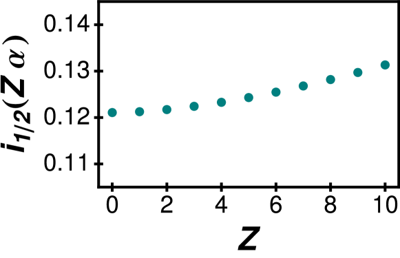
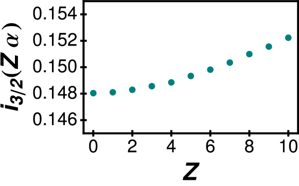
We parameterize the one-loop self-energy correction to the factor of states as
| (43) |
where is the nonperturbative (in ) remainder function. The remainder functions and for and , respectively, have recently been evaluated in Ref. YeJe2010 . Numerical values of for are given in Table Acknowledgments. Note that these data imply a spin-dependence of the higher-order correction term beyond the spin-dependence of the high-energy part given by Eq. (10). The limit as of the remainder function is
| (44) |
As shown in Figs. 1 and 2, this limit is being consistently approached by the numerical data.
References
- (1) S. J. Brodsky and R. G. Parsons, Phys. Rev. 163, 134 (1967).
- (2) R. A. Hegstrom, Phys. Rev. A 7, 451 (1973).
- (3) H. Grotch and R. Kashuba, Phys. Rev. A 7, 78 (1973).
- (4) H. Grotch and R. A. Hegstrom, Phys. Rev. A 8, 2771 (1973).
- (5) J. Calmet, H. Grotch, and D. A. Owen, Phys. Rev. A 17, 1218 (1978).
- (6) J. M. Anthony and K. J. Sebastian, Phys. Rev. A 48, 3792 (1993).
- (7) I. Gonzalo and E. Santos, Phys. Rev. A 56, 3576 (1997).
- (8) Z. C. Yan and G. W. F. Drake, Phys. Rev. A 50, R1980 (1994).
- (9) Z. C. Yan, Phys. Rev. A 66, 022502 (2002).
- (10) K. Pachucki, Phys. Rev. A 69, 052502 (2004).
- (11) M. L. Lewis and V. W. Hughes, Phys. Rev. A 8, 2845 (1973).
- (12) C. Lhuillier, J. P. Faroux, and N. Billy, J. Phys. (Paris) 37, 335 (1976).
- (13) U. D. Jentschura and J. Evers, Can. J. Phys. 83, 375 (2005).
- (14) G. Breit, Nature (London) 122, 649 (1928).
- (15) C. Itzykson and J. B. Zuber, Quantum Field Theory (McGraw-Hill, New York, 1980).
- (16) K. Pachucki, Phys. Rev. A 71, 012503 (2005).
- (17) D. A. Varshalovich, A. N. Moskalev, and V. K. Khersonskii, Quantum Theory of Angular Momentum (World Scientific, Singapore, 1988).
- (18) H. A. Bethe, Phys. Rev. 72, 339 (1947).
- (19) J. Bieroń, F. A. Parpia, C. Froese Fischer, and P. Jönsson, Phys. Rev. A 51, 4603 (1995).
- (20) V. A. Yerokhin, A. N. Artemyev, V. M. Shabaev, and G. Plunien, Phys. Rev. A 72, 052510 (2005).
- (21) U. Jentschura and K. Pachucki, Phys. Rev. A 54, 1853 (1996).
- (22) U. D. Jentschura and C. H. Keitel, Ann. Phys. (N.Y.) 310, 1 (2004).
- (23) B. J. Wundt and U. D. Jentschura, Phys. Rev. A 80, 022505 (2009).
- (24) V. A. Yerokhin and U. D. Jentschura, Phys. Rev. A 81, 012502 (2010).
- (25) W. Quint, B. Nikoobakht, and U. D. Jentschura, Pis’ma v ZhETF 87, 36 (2008), [JETP Lett. 87, 30 (2008)].
- (26) K. Pachucki, U. D. Jentschura, and V. A. Yerokhin, Phys. Rev. Lett. 93, 150401 (2004), [Erratum Phys. Rev. Lett. 94, 229902 (2005)].
- (27) A. R. Edmonds, Angular Momentum in Quantum Mechanics (Princeton University Press, Princeton, New Jersey, 1957).
- (28) S. Salomonson and P. Öster, Phys. Rev. A 40, 5559 (1989).
- (29) V. A. Yerokhin, Phys. Rev. A 78, 012513 (2008).