Abstract

We further consider a probe fermion in a dyonic black hole background in anti–de Sitter spacetime, at zero temperature, comparing and contrasting two distinct classes of solution that have previously appeared in the literature. Each class has members labeled by an integer $n$, corresponding to the $n$th Landau level for the fermion. Our interest is the study of the spectral function of the fermion, interpreting poles in it as indicative of quasiparticles associated with the edge of a Fermi surface in the holographically dual strongly coupled theory in a background magnetic field ${\cal H}$ at finite chemical potential. Using both analytical and numerical methods, we explicitly show how one class of solutions naturally leads to an infinite family of quasiparticle peaks, signaling the presence of a Fermi surface for each level $n$. We present some of the properties of these peaks, which fall into a well behaved pattern at large $n$, extracting the scaling of Fermi energy with $n$ and ${\cal H}$, as well as the dispersion of the quasiparticles.

1 Introduction

Recent work has considerably enriched our detailed knowledge of the kinds of strongly coupled physics that can be studied using holographic studies of charged black holes. Such studies are in fact quite old, since it was realized very shortly after the formulation of the AdS/CFT correspondence [1, 2, 3] that electrically charged black holes allow for the study of non–trivial strongly coupled physics at finite density or chemical potential[4, 5] at both non–zero and zero temperature. A rich phase structure was uncovered in refs.[4, 5], for (finite volume) systems dual to asymptotically AdS spacetime backgrounds with Reissner–Nordström black holes in diverse dimensions. (See also the related work in refs.[6, 7] on the phase structure of certain scalar charged black holes.)

A decade after those studies a new wave of interest emerged, principally due to key observations about how charged black hole solutions to asymptotically AdS Einstein–Maxwell systems (sometimes coupled to scalars and fermions) may pertain directly to holographic models of superconductivity [8, 9, 10] and to holographic access to Fermi surfaces[11, 12]. (Note that the recent focus has been infinite volume system, therefore focusing on flat black holes.)

In the latter case (refs.[11, 12]) the system that displays Fermi surface behaviour is a zero temperature Reissner–Nordström black hole with a probe fermion. The spectral function $G_{R}(\omega,k)$ of the probe fermion in this background was shown, at $T=0$ and finite chemical potential $\mu$, to exhibit a sharp peak at $\omega=0$ and finite $k(=k_{F})$. This peak has been interpreted as the quasiparticle pole at the edge of a Fermi surface. Here $\omega$ is identified with Fermi energy above the chemical potential, $\omega=E_{F}-\mu$. The dispersion associated with this peak was observed to be distinctly non–Landau in a manner consistent with the quasiparticles being not effectively free (as in standard Landau theory), but in a strongly coupled phase. This is encouraging, since this type of behaviour is reminiscent of that which one might hope to gain understanding of in order to gain insight into various novel phenomena known from experiment in condensed matter physics (see for example ref.[13] for a review).

Several concerns arise here. Not the least is that the while the results are suggestive, a quasiparticle peak alone (especially for a minimally coupled non–backreacting fermion) is not damning evidence for a Fermi surface. Some encouragement is to be found in ref. [14] where they showed that at $T\neq 0$ the peak broadened as a function of $T$ in the expected manner, but much more evidence is desirable. Another concern is that the parallel studies of holographic superconductivity in the literature all strongly indicate that a charged scalar profile (representing the condensate/order parameter) would have developed at a critical temperature well above $T=0$, and so an extremal Reissner–Nordström solution is presumably the wrong object to be studying for the $T=0$ physics at $\mu\neq 0$. (In fact, that an extremal black hole is probably excluded from this point of the phase diagram was already suggested a decade ago[4], since there is an expected decay channel due to super–radiance effects[15], inherited from the fact that the charged black holes are really dimensional reductions of spinning D3–branes.) The approximate holographic superconductivity studied in refs. [8, 9, 10] suggest that at $T=0$ the system would be (at best) a scalar–profiled charged black hole (i.e. not Reissner–Nordström) and so one might argue that this is the system to which the spectral analysis should be applied. However, further study in a fully backreacted M–theory context[16, 17, 18, 19] has shown that the black hole nature of the system entirely vanishes at $T=0$. An AdS background re–emerges at $T=0$ instead. This may all fit well with the expectation that if the system has become superconducting below some $T=T_{c}$ the Fermi surface may well no longer be available, although it remains to be seen what the appropriate study might reveal.

With all these concerns up front, it is our view that the work of refs. [11, 12] remains of considerable value. It is a simple, remarkable system with many of the key features of interest for some of the studies, since away from $T=0$, at high enough temperature, a charged black hole will still be relevant. The techniques developed and insights gained in this study, even if the system is not exactly the right one, will be of value in the broader context.

In this spirit, we continue the study that we began of the Reissner–Nordström system and the putative Fermi surface in the presence of a background magnetic field ${\cal H}$. In our first paper[20], we studied a dyonic black hole, the magnetic component now playing the role of an external magnetic field of the system. On general grounds, one expects the system to develop an infinite set of Landau levels, the quantized energy levels of the fermions in the magnetic field. Our first paper studied the lowest Landau level, and already we saw interesting physics, including multiple quasiparticle peaks and a magnetic field dependence in the dispersion characteristic of the peaks.

The non–zero magnetic field case has peaks appearing at $\omega=E_{F}-\mu\neq 0$ since now the energy of the fermions has been increased as compared to the ${\cal H}=0$ system, for a given $\mu$. So even for the lowest Landau level, the peak is at $\omega\neq 0$, as we saw in ref.[20]. This lowest Landau level has a boundary condition for the probe fermion at the horizon that is constructed from the zeroth Hermite function. In this paper we will study more general boundary conditions corresponding to the $n$th Hermite function, and we find a family of quasiparticle peaks signalling the presence of a Fermi surface at each such $n$. Each value of $n$, for fixed chemical potential $\mu$, is a distinct Landau level for the probe fermion.

There are two distinct classes of solution that we present and study here. One class is separable (section 3.1) and the other can be understood as an infinite sum of the separable solutions (section 3.2). The first, adopted in the work of refs.[21, 22], does not have a smooth limit to the ${\cal H}=0$ case (for general momentum $k_{x}$). As a result, we find it less compelling as a basis for the generalization of the results and methods of ref.[11] for the purposes of identifying Fermi surfaces by searching for quasiparticle peaks, since the method requires that the location (in ($\omega,k$)) of the peaks in the spectral function $G_{R}(\omega,k)$ (generically appearing at non–zero $k_{x}$) be read off from the system, and not fixed by hand. We stress that there is nothing wrong with studying the separable class of solutions, for the appropriate kind of physics of interest. Rather, we are noting that it does not connect to the ${\cal H}=0$ physics in a way that allows an analysis of the Fermi surface physics in the spirit of the prototype case of ref.[11]. Following from this, we note in section 3.1 that the choices made in ref.[21], when taken to their logical conclusion (performing the required Fourier transform to construct the spectral function), lead to no quasiparticle peaks at all. By contrast, the infinite–sum class, which we began the study of in ref.[20], has a smooth limit to the ${\cal H}=0$ case, as we discuss in section 3.2, and we carry out the search for quasiparticle peaks and display our results in section 4.

2 Free Fermions in a Magnetic Field

To set the stage and for later comparison with the more complicated case, we begin by studying a free fermion with mass $m$ charged under a global $U(1)$. The Dirac action is:

$$S_{D}=i\int d^{3}x\left(\bar{\Psi}\gamma^{\mu}\mathcal{D}_{\mu}\Psi-m\bar{\Psi}\Psi\right)\ ,$$ (1)

where $\mathcal{D}_{\mu}=\partial_{\mu}-iqA_{\mu}$ is the covariant derivative. The classical equations of motion are given by:

$$\left(\gamma^{\mu}\mathcal{D}_{\mu}-m\right)\Psi=0\ .$$ (2)

Let us first consider the case of zero magnetic field, taking only $A_{t}=-\mu$ to be non–zero. If we choose:

$$\gamma^{0}=-i\sigma_{3}\ ,\quad\gamma^{1}=\sigma_{2}\ ,\quad\gamma^{2}=-\sigma_{1}\ ,$$ (3)

and take an ansatz of the form:

$$\Psi=e^{-i\omega t+ik_{x}x}\left(\begin{array}[]{c}\phi_{+}(\omega,k_{x})\\ \phi_{-}(\omega,k_{x})\end{array}\right)\ ,$$ (4)

then the equations of motion reduce to (for $m=0$):

$$\left(\omega-q\mu\right)\phi_{\pm}-k_{x}\phi_{\mp}=0\ .$$ (5)

The solutions are then given by:

$$k_{x}=\omega-q\mu \mathrm{with} \phi_{+}=\phi_{-}\ ,$$ (6)

$$-k_{x}=\omega-q\mu \mathrm{with} \phi_{+}=-\phi_{-}\ .$$ (7)

Note in particular that at $k_{x}=0$, the non–trivial solution is simply $\omega-q\mu=0$ with no restriction on $\phi_{\pm}(\omega,k_{x})$.

Let us now consider turning on a magnetic field. Taking $A_{x}=-yH$, and following a similar procedure as above (with $\phi_{\pm}$ now depending on $y$ as well), we find as equations of motion:

$$\partial_{y}\phi_{\pm}+m\phi_{\mp}\pm\left(k_{x}+Hqy\right)\phi_{\mp}=\left(\omega-q\mu\right)\phi_{\mp}\ .$$ (8)

Let us assume at present that $Hq>0$ and $m=0$ and define a new coordinate $\eta$ as:

$$\eta=\sqrt{Hq}\left(y+\frac{k_{x}}{Hq}\right)\ ,$$ (9)

in terms of which the equation of motion simplifies to:

$$\sqrt{Hq}\left(\partial_{\eta}\phi_{\pm}\pm\eta\phi_{\mp}\right)=\pm\left(\omega-q\mu\right)\phi_{\mp}\ .$$ (10)

If we consider solutions of the form:

$$\phi_{+}=c(\omega,k_{x})I_{n}(\eta)\ ,\quad\phi_{-}=c(\omega,k_{x})I_{n-1}(\eta)\ ,$$ (11)

where $I_{n}$ are the standard Hermite functions defined in terms of the Hermite polynomials $H_{n}$ as :

$$I_{n}(\eta)\equiv N_{n}H_{n}=\frac{1}{\sqrt{2^{n}n!\sqrt{\pi}}}e^{-\eta^{2}/2}H_{n}(\eta)\ ,$$ (12)

we have the requirement that:

$$\sqrt{2Hqn}=\omega-q\mu\ .$$ (13)

Another solution is given by:

$$\phi_{+}=c(\omega,k_{x})I_{n}(\eta)\ ,\quad\phi_{-}=-c(\omega,k_{x})I_{n-1}(\eta)\ ,$$ (14)

The solutions for the fields are the same as before, but now we have the requirement:

$$-\sqrt{2Hqn}=\omega-q\mu\ .$$ (15)

Let us now consider the case of $Hq<0$. The analysis is mostly the same, except that we now define $\eta$ as:

$$\eta=-\sqrt{-Hq}\left(y+\frac{k_{x}}{Hq}\right)$$ (16)

This modifies the equation of motion to:

$$\sqrt{-Hq}\left(\partial_{\eta}\phi_{\pm}\mp\eta\phi_{\pm}\right)=\mp\left(\omega-q\mu\right)\phi_{\mp}\ .$$ (17)

The solutions to this equation are given by:

$$\left\{\begin{array}[]{c}\phi_{+}(\omega,k_{x},y)=c(\omega,k_{x})I_{n-1}(\eta)\ ,\quad\phi_{-}(\omega,k_{x},y)=c(\omega,k_{x})I_{n}(\eta)\ ,\\ \\ \sqrt{-2Hqn}=\omega-\mu q\ ,\end{array}\right.$$ (18)

and

$$\left\{\begin{array}[]{c}\phi_{+}(\omega,k_{x},y)=c(\omega,k_{x})I_{n-1}(\eta)\ ,\quad\phi_{-}(\omega,k_{x},y)=-c(\omega,k_{x})I_{n}(\eta)\ ,\\ \\ -\sqrt{-2Hqn}=\omega-\mu q\ .\end{array}\right.$$ (19)

In particular, we note that flipping the sign on the magnetic field interchanges the $\eta$ dependence for $\phi_{\pm}$.

Finally, let us study the zero magnetic field limit, which is a delicate issue. We first point out that the coordinate change presented in equation (9) is singular in the limit of zero magnetic field, so it is not a particularly good basis for studying this limit. However, one might think that in order for the restriction on $\omega$ to match, we have to choose:

$$\lim_{H\to 0}\left(\pm\sqrt{2|Hq|n}\right)=\pm k_{x}=\mathrm{fixed}\ .$$ (20)

However, in this limit, the functions $I_{n}$ behave as:

$$I_{n}(\eta)\sim\pi^{-\frac{1}{2}}2^{n-\frac{1}{4}}n^{-\frac{1}{4}}e^{\mp k_{x}y-\frac{n}{2}}\ ,$$ (21)

so both $\phi_{+}$ and $\phi_{-}$ vanish in the limit of large $n$. This does not match the zero magnetic field solution we found earlier. We can perhaps compensate for this vanishing by including an $n$–dependent overall normalization of our fields $\phi_{\pm}$, but we emphasize that this issue is not present when $k_{x}=0$. There, no special limit needs to be taken on $n$ and the Hermite functions go to a constant in the limit of $H\to 0$. This sort of property will occur in our full probe fermion problem later, for one class of solutions (separable) that we will discuss. There will be another class of solutions (infinite–sum) that will not suffer from this limitation, having a smooth $H=0$ limit for arbitrary $k_{x}$. This latter class is naturally amenable to being used to search for Fermi surfaces by looking for quasiparticle peaks in the spectral function, since these peaks will naturally occur at non–zero $k_{x}$ which we wish to read off as output, and not fix a priori.

3 Probing the Black Hole

Our probe is a Dirac fermion in an asymptotically AdS₄ dyonic black hole background. It is charged under the background’s $U(1)$, and the metric and fields are given by:

$$ds^{2} = \frac{L^{2}\alpha^{2}}{z^{2}}\left(-f\left(z\right)dt^{2}+dx^{2}+dy^{2}\right)+\frac{L^{2}}{z^{2}}\frac{dz^{2}}{f\left(z\right)}\ ,$$ (22)

$$F = 2H\alpha^{2}dx\wedge dy+2Q\alpha dz\wedge dt\ ,$$

$$f\left(z\right) = 1+\left(H^{2}+Q^{2}\right)z^{4}-\left(1+H^{2}+Q^{2}\right)z^{3}=\left(1-z\right)\left(z^{2}+z+1-\left(H^{2}+Q^{2}\right)z^{3}\right)\ .$$

The parameter $\alpha$ has dimensions of inverse length. The negative cosmological constant sets the length scale $L$, $\Lambda=-3/L^{2}$, and the Einstein–Maxwell action is:

$$S_{\rm bulk}=\frac{1}{2\kappa_{4}^{2}}\int\!d^{4}x\sqrt{-G}\left\{R+\frac{6}{L^{2}}-\frac{L^{2}}{4}F^{2}\right\}\ ,$$ (23)

where we use signature $(-+++)$, and $\kappa^{2}_{4}=8\pi G_{N}$. The mass per unit volume and temperature of the background are given by:

$$\varepsilon=\frac{\alpha^{3}L^{2}}{\kappa^{2}_{4}}[1+Q^{2}+H^{2}]\ ,\quad T=\frac{\alpha}{4\pi}[3-(Q^{2}+H^{2})]\ .$$ (24)

The coordinates we have chosen above in equation (22) are such that the boundary of AdS₄ (where the dual $(2+1)$–dimensional theory is defined in the ultraviolet) is at $z=0$ while the horizon of the black hole is at $z=1$.

We choose a gauge such that:

$$A_{t}=2Q\alpha(z-1)\ ,\quad\mathrm{and}\quad A_{x}=-2H\alpha^{2}y\ ,$$ (25)

which sets a chemical potential $\mu=-Q\alpha$ and a magnetic field ${\cal H}=-2H\alpha^{2}$. We choose to work at zero temperature, which restricts $Q$ and $H$ to satisfy:

$$H^{2}+Q^{2}=3\ .$$ (26)

As discussed in our first paper[20], it is important to realize that this equation does not place a restriction on the magnetic field for a given value of $Q$. The important quantity to hold fixed while varying the magnetic field is the chemical potential $\mu$, and as $Q$ decreases for increasing $H$, $\alpha$ increases to compensate, resulting in the physical magnetic field ${\cal H}$ being able to run its full natural range from zero to infinity.

Now $z$ is dimensionless in our equations above while all the other coordinates are dimensionful. For convenience, in what follows we will rescale our fields and coordinates to dimensionless quantities:

$$t\to t/\alpha\ ,\quad x\to x/\alpha\ ,\quad y\to y/\alpha\ ,\quad A_{t}\to\alpha A_{t}\ ,\quad\mathrm{and}\,\,A_{x}\to\alpha^{2}A_{x}\ .$$ (27)

The Dirac action for our probe fermion is:

$$S_{D}=i\!\int\!d^{4}x\sqrt{-G}\left({\bar{\Psi}}\Gamma^{M}{\cal D}_{M}\Psi-m{\bar{\Psi}}\Psi\right)\ ,$$ (28)

with the covariant derivative ${\cal D}_{M}$ given by:

$${\cal D}_{M}=\partial_{M}+\frac{1}{4}\omega_{abM}\Gamma^{ab}-iqA_{M}\ ,$$ (29)

where we have used vielbeins $e^{M}_{a}$ to exchange curved spacetime indices $\{M,N\}$ for tangent space indices $\{a,b\}$, and

$$\Gamma^{ab}\equiv\frac{1}{2}[\Gamma^{a},\Gamma^{b}]\ ,\quad\omega_{abM}\equiv e^{N}_{a}\partial_{M}e_{bN}-e_{a\,N}e^{O}_{b}\Gamma^{N}_{OM}\ .$$ (30)

The fermion couples to an operator of dimension $\Delta=m+d/2$ in the $(2+1)$–dimensional theory. We will later choose the case $m=0$ for much of the treatment we will do in this paper. We choose for our Gamma matrices:

$$\Gamma^{t} = \left(\begin{array}[]{cc}-i\sigma_{2}&0\\ 0&-i\sigma_{2}\end{array}\right)\ ,\quad\Gamma^{x}=\left(\begin{array}[]{cc}-\sigma_{3}&0\\ 0&\sigma_{3}\end{array}\right)\ ,$$ (35)

$$\Gamma^{y} = \left(\begin{array}[]{cc}0&-i\sigma_{3}\\ i\sigma_{3}&0\end{array}\right)\ ,\quad\Gamma^{z}=\left(\begin{array}[]{cc}-\sigma_{1}&0\\ 0&-\sigma_{1}\end{array}\right)\ ,$$ (40)

where the $\sigma_{i}$ are the standard Pauli matrices.

We write the Dirac spinor in terms of two 2–component spinors:

$$\Psi^{T}=z^{3/2}f(z)^{-1/4}e^{-i\omega t+ik_{x}x}\left(\phi_{1}\ ,\phi_{2}\right)\ ,$$ (41)

and the equation of motion reduces to:

$$\sqrt{\frac{g_{xx}}{g_{zz}}}\left(\partial_{z}\phi_{{}^{1}_{2}}+\frac{m}{z}\sigma_{1}\phi_{{}^{1}_{2}}\right)+iu\sigma_{3}\phi_{{}^{1}_{2}}\pm\sigma_{2}\left(\partial_{y}\phi_{{}^{2}_{1}}+\left(k_{x}+2Hqy\right)\phi_{{}^{1}_{2}}\right)=0\ ,$$ (42)

with:

$$u=\sqrt{\frac{g_{xx}}{-g_{tt}}}\left(\omega+2qQ(z-1)\right)\ ,\ \sqrt{\frac{g_{xx}}{g_{zz}}}=\sqrt{f}\ ,\sqrt{\frac{g_{xx}}{-g_{tt}}}=\frac{1}{\sqrt{f}}\ .$$ (43)

Near the AdS boundary, the solutions to this equation asymptote to:

$$\lim_{z\to 0}\phi_{{}^{1}_{2}}(y,z)=a_{{}^{1}_{2}}(y)\left(\begin{array}[]{c}1\\ 1\end{array}\right)z^{-m}+b_{{}^{1}_{2}}(y)\left(\begin{array}[]{r}-1\\ 1\end{array}\right)z^{m}\ .$$ (44)

We can define 4–component spinors $\phi_{\pm}$ that have eigenvalues $\pm 1$ under $\Gamma^{z}$:

$$\phi_{\pm}(y,z)=\frac{1}{2}\left(1\pm\Gamma^{z}\right)\Psi(y,z)=\frac{1}{2}\left(\begin{array}[]{c}\left(1\mp\sigma_{1}\right)\phi_{1}(y,z)\\ \left(1\mp\sigma_{1}\right)\phi_{2}(y,z)\end{array}\right)\ .$$ (45)

In the limit of $z\to 0$, $\phi_{\pm}$ asymptote to:

$$\phi_{+}(y,z)=z^{m}\left(\begin{array}[]{r}-b_{1}\\ b_{1}\\ -b_{2}\\ b_{2}\end{array}\right)\ ,\quad\phi_{-}(y,z)=z^{-m}\left(\begin{array}[]{r}a_{1}\\ a_{1}\\ a_{2}\\ a_{2}\end{array}\right)\ .$$ (46)

Using the prescription of ref. [23] to calculate the retarded Green function (the spectral function of interest), we write:

$$\left(\begin{array}[]{r}-\tilde{b}_{1}\\ \tilde{b}_{1}\\ -\tilde{b}_{2}\\ \tilde{b}_{2}\end{array}\right)={\cal S}\left(\begin{array}[]{r}\tilde{a}_{1}\\ \tilde{a}_{1}\\ \tilde{a}_{2}\\ \tilde{a}_{2}\end{array}\right)=\left(\begin{array}[]{cccc}0&-\frac{\tilde{b}_{1}}{\tilde{a}_{1}}&0&0\\ \frac{\tilde{b}_{1}}{\tilde{a}_{1}}&0&0&0\\ 0&0&0&-\frac{\tilde{b}_{2}}{\tilde{a}_{2}}\\ 0&0&\frac{\tilde{b}_{2}}{\tilde{a}_{2}}&0\end{array}\right)\left(\begin{array}[]{r}\tilde{a}_{1}\\ \tilde{a}_{1}\\ \tilde{a}_{2}\\ \tilde{a}_{2}\end{array}\right)\ ,$$ (47)

where $\tilde{a}$ and $\tilde{b}$ are the Fourier transform in the $y$–direction of $a$ and $b$ respectively and hence find for the retarded Green function:

$$G_{R}=-i\mathcal{S}\Gamma^{t}=i\left(\begin{array}[]{cccc}\frac{\tilde{b}_{1}}{\tilde{a}_{1}}&0&0&0\\ 0&\frac{\tilde{b}_{1}}{\tilde{a}_{1}}&0&0\\ 0&0&\frac{\tilde{b}_{2}}{\tilde{a}_{2}}&0\\ 0&0&0&\frac{\tilde{b}_{2}}{\tilde{a}_{2}}\end{array}\right)\ .$$ (48)

The dual (boundary) field theory should have half the components that the bulk theory has, and this is reflected in the Green function by having only two independent terms. Finally, if we write:

$$\phi_{1}=\left(\begin{array}[]{c}A_{1}\\ B_{1}\end{array}\right)\ ,\quad\mathrm{and}\quad\phi_{2}=\left(\begin{array}[]{c}A_{2}\\ B_{2}\end{array}\right)\ ,$$ (49)

then the functions $(a_{{}^{1}_{2}},b_{{}^{1}_{2}})$ can be written:

$$a_{{}^{1}_{2}}(y)=\lim_{\epsilon\to 0}\frac{\epsilon^{m}}{2}\left(B_{{}^{1}_{2}}(y,\epsilon)+A_{{}^{1}_{2}}(y,\epsilon)\right)\ ,\quad b_{{}^{1}_{2}}(y)=\lim_{\epsilon\to 0}\frac{\epsilon^{-m}}{2}\left(B_{{}^{1}_{2}}(y,\epsilon)-A_{{}^{1}_{2}}(y,\epsilon)\right)\ ,$$ (50)

(with analogous expressions for the Fourier transforms $({\tilde{a}},{\tilde{b}})$, with $({\tilde{A}},{\tilde{B}})$ instead of $(A,B)$) such that the relevant Green function quantities are simply:

$$G_{R}^{(1)}(\omega,k_{x},k_{y})=\lim_{\epsilon\to 0}i\epsilon^{-2m}\frac{\tilde{B}_{1}-\tilde{A}_{1}}{\tilde{B}_{1}+\tilde{A}_{1}}\ ,\quad G_{R}^{(2)}(\omega,k_{x},k_{y})=\lim_{\epsilon\to 0}i\epsilon^{-2m}\frac{\tilde{B}_{2}-\tilde{A}_{2}}{\tilde{B}_{2}+\tilde{A}_{2}}\ .$$ (51)

To solve for the fields $A_{{}^{1}_{2}},B_{{}^{1}_{2}}$, we define:

$$A_{{}^{1}_{2}}=e^{i\omega/(6(1-z))}(1-z)^{i(6qQ-4\omega)/18}A_{\pm}\ ,\quad B_{{}^{1}_{2}}=e^{i\omega/(6(1-z))}(1-z)^{i(6qQ-4\omega)/18}B_{\pm}\ .$$ (52)

The equations of motion for the fields $(A_{\pm},B_{\pm})$ when $m=0$ is given by:

$$\sqrt{\frac{g_{xx}}{g_{zz}}}\left(\partial_{z}+\frac{i\omega}{6(1-z)^{2}}+i\frac{-6qQ+4\omega}{18(1-z)}\right)A_{+} = -iuA_{+}+i\left(\partial_{y}B_{-}+(2Hqy+k_{x})B_{+}\right),$$

$$\sqrt{\frac{g_{xx}}{g_{zz}}}\left(\partial_{z}+\frac{i\omega}{6(1-z)^{2}}+i\frac{-6qQ+4\omega}{18(1-z)}\right)A_{-} = -iuA_{-}-i\left(\partial_{y}B_{+}+(2Hqy+k_{x})B_{-}\right),$$

$$\sqrt{\frac{g_{xx}}{g_{zz}}}\left(\partial_{z}+\frac{i\omega}{6(1-z)^{2}}+i\frac{-6qQ+4\omega}{18(1-z)}\right)B_{+} = +iuB_{+}-i\left(\partial_{y}A_{-}+(2Hqy+k_{x})A_{+}\right),$$

$$\sqrt{\frac{g_{xx}}{g_{zz}}}\left(\partial_{z}+\frac{i\omega}{6(1-z)^{2}}+i\frac{-6qQ+4\omega}{18(1-z)}\right)B_{-} = +iuB_{-}+i\left(\partial_{y}A_{+}+(2Hqy+k_{x})A_{-}\right)\ .$$

These are the equations of motion we presented in ref. [20]. Expanding the equations of motion at the event horizon, we find (for $\omega\neq 0$) the following conditions:

$$A_{\pm}(y,1) = 0\ ,$$ (54)

$$\partial_{z}A_{\pm}(y,1) = \mp\frac{\sqrt{6}}{2\omega}\left(k_{x}B_{\pm}(y,1)+\partial_{y}B_{\mp}(y,1)+2HqyB_{\pm}(y,1)\right)\ ,$$ (55)

$$\partial_{z}B_{\pm}(y,1) = \frac{-i}{108}\left(\mp 18\sqrt{6}\left(k_{x}\partial_{z}A_{\pm}(y,1)+\partial_{z}\left(\partial_{y}A_{\mp}(y,1)+2HqyA_{\pm}(y,1)\right)\right)\right.$$ (56)

$$\left.+\left(48qQ-23\omega\right)B_{\pm}(y,1)\right)\ .$$

(There are analogous equations for $\omega=0$, but we do not list them here since we will not find quasiparticle peaks at $\omega=0$.) There is some freedom in choosing the boundary conditions for the fields, leading to very different physics. We present two particular choices in the next two sections.

3.1 Separable Solutions

We restrict ourselves at present to $qH>0$. Changing coordinates to:

$$\eta=\sqrt{2Hq}\left(y+\frac{k_{x}}{2Hq}\right)\ ,$$ (57)

we can write the $y$–dependent parts of our equations above as:

$$\partial_{y}B_{\pm}+(2Hqy+k_{x})B_{\mp} = \sqrt{2Hq}\left(\partial_{\eta}B_{\pm}+\eta B_{\mp}\right)\ ,$$ (58)

$$\partial_{y}A_{\pm}+(2Hqy+k_{x})A_{\mp} = \sqrt{2Hq}\left(\partial_{\eta}A_{\pm}+\eta A_{\mp}\right)\ .$$ (59)

There are two possible ansätze that we can make:

$$\mathrm{ansatz\ 1}:\ A_{-}=-A_{+}=-Y_{A}(y)Z_{A}(z)\ ,\quad B_{-}=B_{+}=Y_{B}(y)Z_{B}(z)\ ,$$ (60)

or

$$\mathrm{ansatz\ 2}:\ A_{-}=A_{+}=Y_{A}(y)Z_{A}(z)\ ,\quad B_{-}=-B_{+}=-Y_{B}(y)Z_{B}(z)\ .$$ (61)

We emphasize that the ansatz with $A_{-}=A_{+}$ and $B_{-}=B_{+}$ is not consistent with the first order equations. Let us start with the first ansatz. If we write:

$$\partial_{\eta}Y_{B}+\eta Y_{B} = \sqrt{2n}Y_{A}\ ,$$ (62)

$$\partial_{\eta}Y_{A}-\eta Y_{A} = -\sqrt{2n}Y_{B}\ ,$$ (63)

then the solution takes the form:

$$Y_{A}=I_{n-1}(\eta)\ ,\quad Y_{B}=I_{n}(\eta)\ ,$$ (64)

where $I_{n}$ is the Hermite function defined in section 2. Note that $I_{-1}=0$. With this ansatz, the equations of motion in the bulk become:

$$\sqrt{\frac{g_{xx}}{g_{zz}}}\left(\partial_{z}+\frac{i\omega}{6(1-z)^{2}}+i\frac{-6qQ+4\omega}{18(1-z)}\right)Z_{A} = -iuZ_{A}+2i\sqrt{Hqn}Z_{B}\ ,$$

$$\sqrt{\frac{g_{xx}}{g_{zz}}}\left(\partial_{z}+\frac{i\omega}{6(1-z)^{2}}+i\frac{-6qQ+4\omega}{18(1-z)}\right)Z_{B} = +iuZ_{B}-2i\sqrt{Hqn}Z_{A}\ .$$ (65)

If we consider the second ansatz, we can write:

$$\partial_{\eta}Y_{B}-\eta Y_{B} = -\sqrt{2n}Y_{A}\ ,$$ (66)

$$\partial_{\eta}Y_{A}+\eta Y_{A} = \sqrt{2n}Y_{B}\ ,$$ (67)

which has solutions given by:

$$Y_{A}(y)=I_{n}(\eta)\ ,\quad Y_{B}(y)=I_{n-1}(\eta)\ ,$$ (68)

and the equations of motion reduce to equations (3.1), the same set of equations of motion that resulted from the first ansatz. So in this case, the behavior in the $z$ direction is independent of our choice. We will return to the issue of this freedom later.

We proceed with calculating the Green function given by equation (51), where all the fields have been Fourier transformed in both $(x,y)$ coordinates. Note that in the analysis of ref. [21], no Fourier transform was performed for the $y$ coordinate. The Fourier transform of the Hermite functions is given by:

$$\int_{-\infty}^{\infty}dye^{-ik_{y}y}I_{n}(\eta)=e^{i\frac{k_{x}}{\sqrt{2Hq}}}\sqrt{\frac{2\pi}{2Hq}}N_{n}(-i)^{n}e^{-\left(\frac{k_{y}}{\sqrt{2Hq}}\right)^{2}/2}H_{n}\left(\frac{k_{y}}{\sqrt{2Hq}}\right)\ ,$$ (69)

where the normalization $N_{n}$ was given in equation (12).

Let us compare to the results and methods of ref. [11], where $H=0$. There, the choice $k_{y}=0$ is made, and we can examine the physics of the solution we have here at $H\neq 0$ for $k_{y}=0$ to see how it connects. If we restrict to $k_{y}=0$, we find that for $n$ odd, the Fourier transform of $I_{n}(\eta)$ vanishes. Therefore, when $n$ is even, only $\tilde{B}_{\pm}(k_{x},k_{y}=0)$ survive when using the first ansatz, whereas only $\tilde{A}_{\pm}(k_{x},k_{y}=0)$ survive when using the second ansatz. When instead $n$ is odd, only $\tilde{A}_{\pm}(k_{x},k_{y}=0)$ survive for the first ansatz and only $\tilde{B}_{\pm}(k_{x},k_{y}=0)$ survive when using the second ansatz. Therefore, if we wish our retarded Green function to be positive, we must use the first ansatz to describe even modes and the second ansatz to describe odd modes. This gives:

$$G_{R}(\omega,k_{x},k_{y}=0)^{(1),(2)}=i\ .$$ (70)

Let us now consider the $H\to 0$ limit of our solutions. As shown earlier for the free fermion in 2+1 dimensions, the Hermite functions in terms of $\eta$ do not have nice behavior as $H\to 0$. Furthermore, the Green function presented above in the $H\to 0$ limit cannot match the results presented in ref. [11], since their results at $H=0$ are a constant only at $k_{x}=0$. Therefore, these results suggest that this choice of solutions (used, crucially, in ref.[21] to discuss Fermi surfaces) is not connected to the pole found in ref. [11] at $H=0$, but they form a separate set of solutions present at non–zero magnetic field.

We complete our discussion of this set of solutions by considering the case of $qH<0$. The coordinate change is now given by:

$$\eta=-\sqrt{-2Hq}\left(y+\frac{k_{x}}{2Hq}\right)\ .$$ (71)

Under the change of variables, the $y$–dependent part becomes:

$$\partial_{y}B_{\pm}+(2Hqy+k_{x})B_{\mp} = -\sqrt{-2Hq}\left(\partial_{\eta}B_{\pm}-\eta B_{\mp}\right)\ ,$$

$$\partial_{y}A_{\pm}+(2Hqy+k_{x})A_{\mp} = -\sqrt{-2Hq}\left(\partial_{\eta}A_{\pm}-\eta A_{\mp}\right)\ .$$ (72)

If we now consider our two ansätz from before, we find that ansatz 1 results in:

$$B_{+}(y,z)=B_{-}(y,z)=Z_{B}(z)I_{n-1}(\eta)\ ,\quad A_{+}(y,z)=-A_{-}(y,z)=Z_{A}(z)I_{n}(\eta)\ ,$$ (73)

and ansatz 2 gives:

$$B_{+}(y,z)=-B_{-}(y,z)=Z_{B}(z)I_{n}(\eta)\ ,\quad A_{+}(y,z)=A_{-}(y,z)=Z_{A}(z)I_{n-1}(\eta)\ .$$ (74)

Both these ansätze give exactly the same equation of motion as before with the appropriate modification under the square root:

$$\sqrt{\frac{g_{xx}}{g_{zz}}}\left(\partial_{z}+\frac{i\omega}{6(1-z)^{2}}+i\frac{-6qQ+4\omega}{18(1-z)}\right)Z_{A} = -iuZ_{A}+2i\sqrt{-Hqn}Z_{B}\ ,$$

$$\sqrt{\frac{g_{xx}}{g_{zz}}}\left(\partial_{z}+\frac{i\omega}{6(1-z)^{2}}+i\frac{-6qQ+4\omega}{18(1-z)}\right)Z_{B} = +iuZ_{B}-2i\sqrt{-Hqn}Z_{A}\ .$$ (75)

In turn this suggests that when $Hq<0$, the even modes are associated with ansatz 2 and the odd modes are associated with ansatz 1. This is the opposite of what occurred when $Hq>0$.

Let us summarize our results so far:

$$qH>0\left\{\begin{array}[]{c}\mathrm{ansatz}\ 1(n\,\,{\rm even})\left(\begin{array}[]{c}Z_{A}I_{n-1}\\ Z_{B}I_{n}\\ -Z_{A}I_{n-1}\\ Z_{B}I_{n}\end{array}\right)\\ \\ \mathrm{ansatz}\ 2(n\,\,{\rm odd})\left(\begin{array}[]{c}Z_{A}I_{n}\\ Z_{B}I_{n-1}\\ Z_{A}I_{n}\\ -Z_{B}I_{n-1}\end{array}\right)\end{array}\right.\ ,\ qH<0\left\{\begin{array}[]{c}\mathrm{ansatz}\ 1(n\,\,{\rm odd})\left(\begin{array}[]{c}Z_{A}I_{n}\\ Z_{B}I_{n-1}\\ -Z_{A}I_{n}\\ Z_{B}I_{n-1}\end{array}\right)\\ \\ \mathrm{ansatz}\ 2(n\,\,{\rm even})\left(\begin{array}[]{c}Z_{A}I_{n-1}\\ Z_{B}I_{n}\\ Z_{A}I_{n-1}\\ -Z_{B}I_{n}\end{array}\right)\end{array}\right.\ .$$ (76)

Note the close similarity between these results and the results found for the free fermion in $2+1$ dimensions. We find here that for a given ansatz, the single Dirac spinor in the $(3+1)$–dimensional background contains both solutions that were found for the free fermion. Under the flip of the magnetic field for a given ansatz, we find the same flipping of the $\eta$ dependence between each 2–component spinors. In addition, the flipping of the magnetic field interchanges the roles of the two ansätze for describing the modes, which suggests that they may describe aligned vs. anti–aligned couplings. These results indicate that the even modes and odd modes should be understood as describing two distinct ladders.

3.2 Infinite–Sum Solutions

The separable solutions presented so far have two unfortunate features. Because of the solutions’ dependence on the coordinate $\eta$, the solutions have singular behavior in the zero magnetic field limit. To connect these solutions to the zero magnetic field solution, one has to take a limit similar to that of equation (20), where the Landau level label $n$ goes to infinity:

$$\lim_{H\to 0,n\to\infty}\sqrt{4Hqn}=k_{x}$$ (77)

Independent of this fact, considering the separable solutions alone leads to a trivial Green function, as presented in equation (70).

We wish to proceed by studying a class of solutions that avoids these two features. In order to avoid singularities associated with the coordinate $\eta$ , we wish to consider solutions that depend on the coordinate $y$ as opposed to $\eta$. Let us take the case of $Hq>0$. Motivated by the separable solutions discussed earlier, focusing on the behaviour at the horizon ($z=1$), we consider $B_{\pm}(y,1)=B(y,1)$ for even $n$ and $B_{+}=-B_{-}=B(y,1)$ for odd $n$. For $n$ even we take:

$$\partial_{y}B(y,1)+2HqyB(y,1)=\sqrt{4Hqn}B_{0}(1)I_{n-1}(\sqrt{2Hq}y)\ ,$$ (78)

such that we have $B(y,1)=B_{0}(1)I_{n}(\sqrt{2Hq}y)$. We can write this ansatz in terms of our separable solutions from the previous section,

$$B_{+}(y,z)=\sum_{n=0}^{\infty}b_{+}^{(n)}Z_{B}^{(n)}(z)I_{n}(\eta)\ ,$$ (79)

and similarly for the other fields. The coefficients $b_{+}^{(n)}$ can be determined from the field behavior at the event horizon. For example, for $B(y,1)=I_{0}(\sqrt{2Hq}y)$, the coefficients $b_{+}^{(n)}$ are given by:

$$b_{+}^{(n)}=\frac{k_{x}^{n}}{2^{n}\sqrt{\left(Hq\right)^{n}n!}}e^{-\frac{k_{x}^{2}}{8Hq}}\ .$$ (80)

In the limit of $H\to 0$, the infinite sum remains finite without requiring us to take a limit of the form of equation (77). We do not need to take $n\to\infty$ since the infinite sum effectively does this by defining a new Landau level labeling in terms of an infinite sum of the Landau labels of the separable solutions (i.e. the labeling of $I_{n}(\sqrt{2Hq}y)$ instead of $I_{n}(\eta)$). Because of the nature of the infinite sum, it is important to first perform the sum and then take the limit of $H\to 0$ to ensure the correct result. We emphasize that the infinite sum gives us the freedom to vary the new Landau level label as well as $k_{x}$ independently while sending $H\to 0$, a freedom we did not have with the separable solutions presented earlier. This is an important difference from the separable solutions we considered in the previous section.

By substituting the series form of the fields from equation (79) into the equations of motion, the partial differential equation becomes an infinite series of coupled ordinary differential equations for $Z_{A,B}^{(n)}$, where the coupled equations are identical to those of equations (3.1). We have traded the partial differential equation for an infinite number of coupled ordinary differential equations. We choose to proceed by solving the partial differential equation using an ansatz that is not explicitly separable since this is more tractable numerically.

With this ansatz, we find that:

$$\partial_{z}A_{\pm}(y,1)=\mp\frac{\sqrt{6}}{2\omega}\left(k_{x}I_{n}(\sqrt{2Hq}y)+\sqrt{4Hqn}I_{n-1}(\sqrt{2Hq}y)\right)B_{0}(1)\ .$$ (81)

We notice that for $k_{x}=0$, we find that $\partial_{z}A_{\pm}(y,1)\propto I_{n-1}(\sqrt{2Hq}y)$, which agrees with the separable solution from the previous section. Finally, we have:

$$\partial_{z}B_{\pm} = \frac{-iB_{0}(1)}{108}\left(\frac{54}{\omega}\left(k_{x}^{2}I_{n}+k_{x}\sqrt{4Hqn}I_{n-1}+k_{x}\sqrt{4Hq(n+1)}I_{n+1}+4HqnI_{n}\right)\right.$$ (82)

$$\left.+\left(48qQ-23\omega\right)I_{n}\right)\ ,$$

where we have used that:

$$\partial_{y}I_{n}(\sqrt{2qH}y)-2qHyI_{n}(\sqrt{2qH}y)=-\sqrt{4qH(n+1)}I_{n+1}\ .$$ (83)

Note again that for $k_{x}=0$, we recover that $\partial_{z}B_{\pm}(y,1)\propto I_{n}(\sqrt{2Hq}y)$ which is the single separable solution presented earlier. In addition, note that for $n=0$ we recover the equations that we had in ref. [20]. For $n$ odd, we take:

$$\partial_{y}B(y,1)-2HqyB(y,1)=-\sqrt{4Hqn}B_{0}(1)I_{n}(\sqrt{2Hq}y)\ ,$$ (84)

such that we have $B(y,1)=B_{0}(1)I_{n-1}(\sqrt{2Hq}y)$. With this ansatz, we find that:

$$\partial_{z}A_{\pm}(y,1) = -\frac{\sqrt{6}}{2\omega}\left(k_{x}I_{n-1}(\sqrt{2Hq}y)+\sqrt{4Hqn}I_{n}(\sqrt{2Hq}y)\right)B_{0}(1)\ ,$$

$$\partial_{z}B_{\pm} = \mp\frac{iB_{0}(1)}{108}\left(\frac{54}{\omega}\left(k_{x}^{2}I_{n-1}+k_{x}\sqrt{4Hqn}I_{n}+k_{x}\sqrt{4Hq(n-1)}I_{n-2}+4HqnI_{n-1}\right)\right.$$ (85)

$$\left.+\left(48qQ-23\omega\right)I_{n-1}\right)\ .$$

The advantage of this choice over the finitely separable choice from the previous section is that in the $H\to 0$ limit, the equations of motion and fields reduce to those of ref.[11] with no restrictions placed on $n$. In addition, since at $k_{x}=0$, the fields reduce to the simple separable case discussed earlier, we can immediately write the Green function for this special case:

$$G_{R}(\omega,k_{x}=0,k_{y}=0)^{(1),(2)}=i\ ,\qquad\forall H\ ,$$ (86)

which connects nicely with the zero magnetic field ${\vec{k}}=0$ result of ref.[11]. Furthermore, for $k_{x}\neq 0,\ k_{y}=0$, the Green function gives a non–trivial result, as opposed to the separable case which gave a trivial result (see equation (70)).

This infinite–sum class of solutions, which we studied in ref.[20] at $n=0$, is a more natural generalization of the results of ref.[11] and better adapted to the method of searching for new quasiparticle peaks, which generically appear at non–zero $k_{x}$.

3.3 Comments about Complex $\omega$

Before proceeding with our numerical results, we would like to make a few comments about the variable $\omega$. In the usual AdS/CFT dictionary, it is important to recall that $\omega$ is generally complex:

$$\omega=\omega_{\ast}-i\Gamma$$ (87)

The quantity $\Gamma$ is related to the inverse lifetime of the quasinormal mode and $\omega_{\ast}$ is related to the energy of the mode. The imaginary part of $\omega$ must be negative in order for the mode to be stable. In addition, in order for the pole in the Green function to be associated with a quasiparticle, the pole must have non–zero residue. In our analysis, we restrict ourselves to $\Gamma=0$, and therefore our search for poles is such that the lifetime of the mode is always infinite. Away from the poles, the numerical results should not be taken too seriously since away from the poles, one should consider a complex $\omega$ and not a purely real $\omega$. This is relevant because in our numerics the poles occur immediately after a region where the imaginary part of the Green function is negative, which is not allowed if the theory is unitary. We believe that the proper treatment of the complex $\omega$ in these regions would resolve this. In particular, the analysis in ref. [22] shows that the pole for $H=0$ bounces off the real axis, and in the purely real analysis the imaginary part of the Green function remains positive on both sides of the pole. Therefore, our result suggests that the bounce does not occur at the real axis but somewhere in the positive imaginary $\omega$ regime. This suggests that for $\mathrm{Re}(\omega)$ less than our pole, the mode is unstable. In addition, we have not calculated the residue of our poles as this is impossible without having the full complex $\omega$ description of the quasinormal modes. Therefore, our poles have not been shown conclusively to be quasiparticles. However, in ref. [20], the pole studied there was the direct perturbation of the quasiparticle pole in ref. [11] under a magnetic field (meaning that zero magnetic field limit matched) and the perturbed pole occurred at non–zero $\omega$. In that case, since the $H=0$ pole was a quasiparticle, it followed that the $H\neq 0$ pole would also be a quasiparticle. Therefore, in the analysis that is presented next, the fact that the poles occur at non–zero $\omega$ is not entirely surprising, and they have a chance of being real quasiparticle excitations.

4 Numerical Results for the Quasiparticle Spectrum

We employ the numerical methods that we presented in our earlier paper[20] to seek solutions and explicitly construct the spectral function $G_{R}(\omega,k)$, using the more general boundary conditions we have discussed in section 3.2 for the infinite–sum class of solutions. We refer the reader there for the details of our methods, and here present our observations.

First, we notice that for the first four $n$, ($n=0,\ldots,3$) we find two peaks (signalling the presence of poles in the spectral function) for a given $n$. We observed the pair at $n=0$ in our earlier paper[20], and this structure persists for a few levels before disappearing, leaving only single poles for every $n$ beyond $n=3$. In each case where there is a pair, the poles fall into two classes. One class appears to be a deformation of the prototype pole found in ref. [11]. This type is found at smaller $\omega$. The other, found at larger $\omega$ and $k_{x}$, appears to be in the same class as the lone poles present at large $n$, fitting into a smooth curve of progression. We present the first class of poles in figure 1 and the second class of poles in figure 1(b). In all figures, $\omega_{*}$ is used to denote the value of $\omega$ at which the peak is located. (In both figures we colour code even $n$ poles with blue and odd $n$ with red.) Notice that for the first class of poles the even $n$ poles are at higher $\omega$ while for the second class of poles it is the other way around.

Figure 1: The first (finite) class of peaks for a specific value of magnetic field set by $H=-0.1$.

The behavior of the first poles (at $n=0$) was studied extensively in ref. [20] as a function of $H$, and we expect similar behaviour here for $n=1,2,3$. Therefore we focus on the second class of poles, which persists for all Landau levels $n$, in what follows. We present some results for fixed $H$ and varying $n$ in figure 1(b). (Recall that the physical magnetic field is ${\cal H}=-2\alpha^{2}H$.) We note that the behavior of the poles in $\omega_{*}$ vs. $n$ becomes more predictable at higher $n$. In addition, we note that for $Hq>0$, we find that the solutions with ansatz 2 (associated with the odd $n$s) have a larger $\omega_{\ast}$ than the solutions with ansatz 1 (associated with the even $n$s).

(a)

(b) The second class of peaks for a specific value of magnetic field set by $H=-0.1$. (a) The dependence on Fermi momentum. (b) The dependence on Landau level number.

In figure 2 we plot the behavior of the poles at fixed $n$ for varying $H$, for a few sample values of $n$, choosing of $n$ such that it falls in the regime where $\omega_{*}$ behaves regularly with $n$.

(c) $n=10$

(d) $n=20$

(e) $n=30$

Figure 2: Behavior with increasing $H$ for the poles in the regular regime. The best fit line is given by equation (88).

Using these (and much more) data, we can attempt to fit the behavior of $\omega_{\ast}$ with the magnetic field and $n$, for large $n$, giving:

$$\omega_{\ast}\sim 0.71\,\,H^{0.65}n^{0.63}\ .$$ (88)

For how well this function fits the data, see figure 2. In particular, we find that the fit improves for larger $H$ and larger $n$. The exact numbers associated with the scaling of $H$ and $n$ are not as important as the fact that they deviate from the free relativistic fermion behavior which would have both scaling with exponent $1/2$.

Another important characteristic of these poles is the rate at which the peak is approached as a function of $k_{x}$. This is the dispersion of the quasiparticles associated with that peak, and it can be read off from our numerical searches quite readily. In our earlier paper[20], we found that non–zero $H$ modified the behaviour seen in ref.[11]. In particular, a peak at higher $k_{x}$ had more linear (i.e. Landau–like) dispersion. We observe that the same is true for all $n$. Note however that from figure 1(b) it can be seen that, for the second class of peaks (the one that persist for all $n$), at higher $n$, the peaks are at successively lower values of $k_{x}$ (in either the even or odd $n$ sequence). We show some sample dispersion behavior of the poles at fixed $H$ but different $n$ in figure 3.

(a) $n=0$

(b) $n=1$

(c) $n=10$

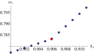
(d) $n=11$

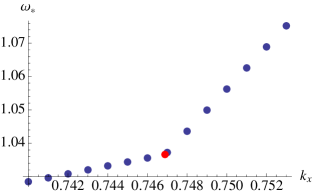
(e) $n=20$

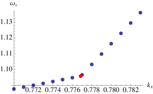
(f) $n=21$

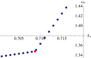
(g) $n=30$

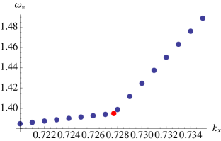
(h) $n=31$

Figure 3: Dispersion behavior near the pole. The red dot marks the position of the pole.

5 Conclusions

We have generalized the work of ref. [20] to include an infinite number of excitations labeled by $n$. Different $n$ correspond to different Landau Levels for the probe fermion in the presence of magnetic field. We studied in detail two separate classes of solution, leading to distinct physics. One class is separable (it is used in the work of refs.[21, 22]) and the other is an infinite sum of the separable solutions (studied for $n=0$ in our first paper[20]). Both classes are probably physical, but the first class does not allow a smooth $H=0$ limit for arbitrary $k_{x}$, and so seems less suitable for discussion of quasiparticle peaks and Fermi surfaces in the spirit of ref.[11], which is our focus (and that of ref.[21]). In fact, we argued that the separable solutions have a constant Green function at $k_{y}=0$ when the $y$–dependence is included in the Green function definition, which differs from the argument presented in ref. [21].

The infinite–sum solutions have key properties that make them attractive. They limit to the $H=0$ solution smoothly for arbitrary $n$, with non–trivial dependence on $k_{x}$. This is the class of solutions we use to find quasiparticle peaks for all the Landau Levels $n$. Note that since $\omega$ depends on $k_{x}$, these Landau levels do not have the usual degeneracy found for the free fermion Landau levels.

We also noted that levels given by even $n$ and odd $n$ form distinct towers, distinguished by a relative energy shift (that diminishes as $n$ increases) that suggests a aligned/anti–aligned coupling to the magnetic field. The difference between even and odd stems from two different choices one can make at the event horizon.

We also noticed that the family of quasiparticle peaks, at sufficiently large $n$, has a dependence on $H$ and $n$ that is different that of the relativistic massless free fermion. In fact the exponent lies between the free relativistic value of $1/2$ and the non–relativistic value of unity. This is consistent with our quasiparticles possibly having an induced mass.

Acknowledgements

We would like to thank Nikolay Bobev, José Barbon, Karl Landsteiner, Moshe Rozali, and Julian Sonner for useful conversations. We would also like to thank an anonymous referee of J. Phys. A. for helpful suggestions for improvement of this manuscript. This work was supported by the US Department of Energy.

References

- [1] J. M. Maldacena, “The large N limit of superconformal field theories and supergravity,” Adv. Theor. Math. Phys. 2 (1998) 231–252, hep-th/9711200.
- [2] E. Witten, “Anti-de Sitter space and holography,” Adv. Theor. Math. Phys. 2 (1998) 253–291, hep-th/9802150.
- [3] S. S. Gubser, I. R. Klebanov, and A. M. Polyakov, “Gauge theory correlators from non-critical string theory,” Phys. Lett. B428 (1998) 105–114, hep-th/9802109.
- [4] A. Chamblin, R. Emparan, C. V. Johnson, and R. C. Myers, “Charged AdS black holes and catastrophic holography,” Phys. Rev. D60 (1999) 064018, hep-th/9902170.
- [5] A. Chamblin, R. Emparan, C. V. Johnson, and R. C. Myers, “Holography, thermodynamics and fluctuations of charged AdS black holes,” Phys. Rev. D60 (1999) 104026, hep-th/9904197.
- [6] M. Cvetic and S. S. Gubser, “Phases of R-charged black holes, spinning branes and strongly coupled gauge theories,” JHEP 04 (1999) 024, hep-th/9902195.
- [7] M. Cvetic and S. S. Gubser, “Thermodynamic stability and phases of general spinning branes,” JHEP 07 (1999) 010, hep-th/9903132.
- [8] S. S. Gubser, “Breaking an Abelian gauge symmetry near a black hole horizon,” 0801.2977.
- [9] S. A. Hartnoll, C. P. Herzog, and G. T. Horowitz, “Holographic Superconductors,” JHEP 12 (2008) 015, 0810.1563.
- [10] S. A. Hartnoll, C. P. Herzog, and G. T. Horowitz, “Building a Holographic Superconductor,” Phys. Rev. Lett. 101 (2008) 031601, 0803.3295.
- [11] H. Liu, J. McGreevy, and D. Vegh, “Non-Fermi liquids from holography,” 0903.2477.
- [12] T. Faulkner, H. Liu, J. McGreevy, and D. Vegh, “Emergent quantum criticality, Fermi surfaces, and AdS2,” 0907.2694.
- [13] C. M. Varma, Z. Nussinov, and W. van Saarloos, “Singular Fermi Liquids,” Physics Reports 361 (2002) 267.
- [14] M. Cubrovic, J. Zaanen, and K. Schalm, “Fermions and the AdS/CFT correspondence: quantum phase transitions and the emergent Fermi-liquid,” 0904.1993.
- [15] R. Penrose, “Gravitational collapse: The role of general relativity,” Riv. Nuovo Cim. 1 (1969) 252–276.
- [16] J. P. Gauntlett, J. Sonner, and T. Wiseman, “Holographic superconductivity in M-Theory,” Phys. Rev. Lett. 103 (2009) 151601, 0907.3796.
- [17] S. S. Gubser, C. P. Herzog, S. S. Pufu, and T. Tesileanu, “Superconductors from Superstrings,” Phys. Rev. Lett. 103 (2009) 141601, 0907.3510.
- [18] S. S. Gubser, S. S. Pufu, and F. D. Rocha, “Quantum critical superconductors in string theory and M- theory,” Phys. Lett. B683 (2010) 201–204, 0908.0011.
- [19] J. Gauntlett, J. Sonner, and T. Wiseman, “Quantum Criticality and Holographic Superconductors in M- theory,” 0912.0512.
- [20] T. Albash and C. V. Johnson, “Holographic Aspects of Fermi Liquids in a Background Magnetic Field,” 0907.5406.
- [21] P. Basu, J. He, A. Mukherjee, and H.-H. Shieh, “Holographic Non-Fermi Liquid in a Background Magnetic Field,” 0908.1436.
- [22] F. Denef, S. A. Hartnoll, and S. Sachdev, “Quantum oscillations and black hole ringing,” 0908.1788.
- [23] N. Iqbal and H. Liu, “Real-time response in AdS/CFT with application to spinors,” 0903.2596.