The role of center vortices in Gribov’s confinement scenario

Abstract

The connection of Gribov’s confinement scenario in Coulomb gauge with the center vortex picture of confinement is investigated. For this purpose we assume a vacuum wave functional which models the infrared properties of the theory and in particular shows strict confinement, i.e. an area law of the Wilson loop. We isolate the center vortex content of this wave functional by standard lattice methods and investigate their contributions to various static propagators of the Hamilton approach to Yang-Mills theory in Coulomb gauge. We find that the infrared properties of these quantities, in particular the infrared divergence of the ghost form factor, are dominated by center vortices.

1 Introduction

The infrared sector of QCD, in particular the confinement mechanism, is not fully understood yet, although substantial progress had been made during recent years. The progress comes mainly from lattice calculations [1], [2], which gave support to both the dual Meissner effect [3] and the center vortex picture [4] of confinement and also indicate that these two pictures are likely only two sides of the same medal. Furthermore, there is lattice evidence that also Gribov’s confinement scenario is triggered by magnetic monopoles and center vortex configurations [5, 6]. In addition, one can show analytically that Zwanziger’s horizon condition, i.e. an infrared diverging ghost form factor, which is at the heart of Gribov’s confinement scenario in Coulomb gauge, implies dual Meissner effect [7].

In recent years there has been a renewed interest in studying Yang-Mills theory in Coulomb gauge, both in the continuum [8] and on the lattice [9, 10, 11, 12, 13, 14]. In particular, much work was devoted to a variational solution of the Yang-Mills Schrödinger equation in Coulomb gauge [15, 16, 17, 18, 19, 20, 21, 22, 23]. Using Gaussian type of Ansatzes for the vacuum wave functional, a set of Dyson-Schwinger equations for the gluon and ghost propagators was derived by minimizing the vacuum energy density. An infrared analysis [22] of these equations exhibits solutions in accord with Gribov(-Zwanziger) confinement scenario. Imposing Zwanziger’s horizon condition one finds an infrared diverging gluon energy and a linear rising static quark (Coulomb) potential [22] and also a perimeter law for the ’t Hooft loop [23]. These infrared properties are reproduced by a full numerical solution of the Dyson-Schwinger equations over the entire momentum regime [19], and are also supported by lattice calculations [10, 13, 14]. Moreover, these lattice calculations also show clear evidence for an infrared divergent ghost form factor and an infrared suppressed static gluon propagator. While the horizon condition has to be imposed by hand in $D=3+1$, as there exist also subcritical solutions with an infrared finite ghost form factor [20], the coupled set of Dyson-Schwinger equations in $D=2+1$ only allows for critical solutions having an infrared diverging ghost form factor [24]. Furthermore, recent studies within the functional renormalization group treatment of the Hamilton approach in Coulomb gauge yields the horizon condition as a solution of the flow equation [25]. In $D=1+1$, finally, the exact ghost form factor is infrared enhanced [21].

Despite the encouraging results for the infrared properties of the various Greens function (in particular the linear Coulomb potential) and the good agreement of the gluon energy [20] with the lattice data [13, 14], the crucial test for the wave functional in the variational approach, namely the calculation of the Wilson loop, still has to come. In fact, a linear Coulomb potential is necessary but not sufficient for confinement since the Coulomb string tension is only an upper bound to the Wilsonian string tension [8]. With the variational vacuum wave functional at hand it would be, in principle, straightforward to calculate the Wilson loop. However, path ordering makes an exact evaluation of the Wilson loop impossible. In Ref. [26] the spatial Wilson loop was calculated from a Dyson equation, which takes care of the path ordering in an approximate fashion, employing the static gluon propagator as input. Despite the rather limited range of applicability of the Dyson equation, a linearly rising potential could be extracted from the obtained Wilson loop.

Here we will proceed along a different line. We assume a wave functional which is known a priori to produce an area law for the (spatial) Wilson loop, and calculate with this wave functional the various propagators of the Hamiltonian approach in Coulomb gauge. The infrared properties of these propagators are then compared with the ones obtained from lattice results in $D=4$ Coulomb gauge which, in turn, agree qualitatively with findings from a Gaussian type of variational wave functional.

A simple choice for a confining wave functional is

$$\Psi[\mathbf{A}]={\cal N}\exp\left(-\frac{1}{8\mu}\int d^{3}xF_{ij}(\mathbf{x})\,F_{ij}(\mathbf{x})\right)\hskip 2.84544pt,$$ (1)

where $F_{ij}$ denotes the spatial components of the non-Abelian field strength and $\mu$ is a dimensionfull parameter, which, in principle, could serve as variational parameter. We will later see that the scaling properties of $D=3$ Yang-Mills theory tie the parameter $\mu$ to the numerical value of the (spatial) string tension: $\mu$ thus merely sets the overall scale.

The wave functional in eq. (1) models the infrared sector of the Yang-Mills vacuum: it is gauge invariant and can be considered as the leading order in a gradient expansion of the true Yang-Mills vacuum wave functional [27]. Furthermore, the functional of eq. (1) produces an area law for the (spatial) Wilson loop. This is because the $D=4$ expectation value of any gauge invariant and $A_{0}$–independent observable $\Omega[\mathbf{A}]$ in this state is precisely given by the one in the $D=3$ dimensional Yang-Mills theory,

$$\langle\,\Psi\,|\,\Omega\,|\,\Psi\rangle=\frac{\displaystyle\int\mathscr{D}\mathbf{A}\,\,\Omega[\mathbf{A}]\,\exp\left[\displaystyle-\frac{1}{4\mu}\int d^{3}xF^{2}_{ij}(\mathbf{x})\right]}{\displaystyle\int\mathscr{D}\mathbf{A}\,\exp\left[-\displaystyle\frac{1}{4\mu}\int d^{3}xF^{2}_{ij}(\mathbf{x})\right]}\,.$$ (2)

For gauge variant observables such as the Green functions, we need to pick a specific gauge on the vector potential $\mathbf{A}$. Choosing Coulomb gauge $\nabla\,\mathbf{A}=0$ in $D=4$ obviously entails Landau gauge for the $D=3$ YM-theory.

The wave functional of eq. (1) is certainly inappropriate at large momenta where it yields a gluon energy $\omega(|\mathbf{k}|)\sim|\mathbf{k}|^{2}$ instead of $\omega(\mathbf{k})\sim|\mathbf{k}|$. However, this should be irrelevant for the confining properties. Also in the deep IR region one does not expect eq. (1) to exactly reproduce the $D=4$ Yang-Mills Theory, since the standard lattice gluon and ghost propagator in $D=3$ Landau gauge rather satisfy a decoupling type of solution [28], in contrast to $D=4$ Coulomb gauge [13, 14]. Indeed, one would expect the correct wave-function to be better described by [29]:

$$\Psi[\mathbf{A}]={\cal N}\exp\left(-\frac{1}{2}\int d^{3}xF_{ij}(\mathbf{x})\frac{1}{\sqrt{-D^{2}+c}}F_{ij}(\mathbf{x})\right)\hskip 2.84544pt,$$ (3)

where $D^{2}$ is the adjoint covariant Laplace operator. In Ref. [29], where the $D=2+1$ theory was examined, the choice $c=-\lambda_{0}+m^{2}$ was made, $\lambda_{0}$ being the lowest eigenvalue of $-D^{2}$. The technical difficulties of working with eq. (3) are however beyond the scope of this paper, since one does not expect the Laplacian term to modify the vortex content of the $D=3$ theory. Even the simplified version given in eq. (1) cannot be used for analytic calculations; instead, the calculation of expectation values in this state requires conventional 3-dimensional Yang-Mills lattice simulations. As stated earlier, these $D=3$ lattice calculations must be carried out in Landau gauge when (1) is used as Schrödinger wave functional in Coulomb gauge.

The infrared properties of the vacuum sector of Yang-Mills theory are known to be dominated by center vortices [1]. This is also true in $D=3$. The wave functional eq. (1) thus contains, among other configurations, an ensemble of percolating center vortices. By standard lattice methods [30] we can extract the center vortex content of this wave functional. Therefore the use of the wave functional eq. (1) also allows us to study (on the lattice) how, within the Hamiltonian approach, the Gribov-Zwanziger confinement mechanism is related to the center vortex picture of confinement. Previous lattice calculations [5, 6] have shown that removal of center vortices from the (4-dimensional) Yang-Mills ensemble by the method of Ref. [30] makes the ghost form factor infrared finite, analogously to the suppression observed before in Landau gauge [31]. In the present work we will calculate the center vortex contribution to various Coulomb gauge propagators. The paper is organized as follows:

In the next section, we briefly recall some properties of $D=3$ Yang–Mills theory, in particular the scaling behavior and some known facts about Landau gauge Green functions. Section 3 contains a description of our numerical setup and the results for the static gluon and ghost form factors in Coulomb gauge. We also discuss the role of center vortices and their implications for the Gribov–Zwanziger scenario. We close with a brief summary and an outlook on future investigations.

2 Yang-Mills theory in three dimensions

Since we want to describe the continuum model of eq. (1) using a lattice, we must first have a closer look at the scaling properties of $D=3$ YM theory. The lattice model is defined on a $D=3$ cubic space-time grid with periodic boundary conditions. We will use the Wilson action and employ various gauge fixing algorithms. The scale $\mu$ of the continuum wave functional in eq. (1) plays the role of the three-dimensional bare YM coupling in the continuum limit, $\mu=g_{0}^{2}$.

In three-dimensional YM theory, the renormalized coupling $g_{R}$ is

$$\beta=\frac{4}{ag_{0}^{2}}\,,\qquad\qquad g_{0}^{2}=g_{R}^{2}\left[1+\mathscr{O}(\hbar\beta^{-1})\right]$$

in terms of the bare coupling $g_{0}$ and the lattice spacing $a$. The string tension in units of the lattice spacing is therefore

$$\hat{\sigma}\equiv\sigma a^{2}=\sigma\,\frac{16}{\beta^{2}g_{0}^{4}}=\frac{16\,\sigma}{\beta^{2}\,g_{R}^{4}}\,+\mathscr{O}(\beta^{-3})\,.$$ (4)

Since $g_{R}$ sets the overall scale, $\sigma/g_{R}^{4}$ is a dimensionless constant independent of $\beta$, i.e. large Creutz ratios should scale according to

$$\chi(R,R)\approx\hat{\sigma}(\beta)=\frac{{\rm const}}{\beta^{2}}+\mathscr{O}(\beta^{-3})\,.$$ (5)

Large-scale simulations in $SU(2)$ [32] have indeed confirmed the existence of a scaling window $\beta\approx 3\ldots 12$ in which the dependency (5) can be observed. More precisely, the best fit [32] is

$$\hat{\sigma}(\beta)=\frac{1.788}{\beta^{2}}\,\left(1+\frac{1.414}{\beta}+\cdots\right)\,.$$ (6)

valid for $\beta\geq 3$. From eqs. (4), (6) and $\mu=g_{0}^{2}$, we find

$$\frac{\sigma}{\mu^{2}}=0.111\,\left[1+\frac{1.414}{\beta}+\cdots\right]\,,$$ (7)

i.e. the variation parameter $\mu=\mu(\sigma,\beta)$ is fixed once the overall scale $\sigma$ and the lattice coupling $\beta$ in the scaling window are given. For the standard value $\sqrt{\sigma}=440\,\mathrm{MeV}$, $\mu$ falls in the range $\mu=1088\,\mathrm{MeV}\,\,\ldots\,\,1236\,\mathrm{MeV}$ when $\beta$ is varied in the scaling window. There is however no compelling reason for the string tension of this $D=3$ model of the $D=4$ Yang-Mills vacuum to coincide with the "physical" string tension of the genuine $D=3$ Yang-Mills theory. In view of the following we will then treat $\mu$ as an adjustable parameter that controls the tradeoff between matching the $D=4$ string tension or the corresponding Green functions.

Ghost and gluon Green functions in Landau gauge are generally expected to be multiplicatively renormalizable, i.e. the lattice data for different $\beta$ must fall on top of each other once the momentum is expressed in physical units and a finite field renormalization $Z(\beta)$ is applied. The Gribov-Zwanziger confinement criterion makes qualitative predictions about the deep IR behavior of Green functions. It is based on the idea that the gauge field configurations in the functional integral should be restricted to the so-called fundamental modular region (FMR). The dominant contributions within the FMR should then come from field configurations near the Gribov horizon, where the near-zero modes of the Faddeev-Popov operator $\mathsf{M}\equiv-\partial\hat{D}$ strongly enhance the Coulomb potential

$$V_{c}(|\mathbf{x}-\mathbf{y}|)\sim\mathrm{Tr}\,\left\langle\mathsf{M}^{-1}\,(-\Delta)\,\mathsf{M}^{-1}\right\rangle.$$ (8)

To enforce the restriction to the FMR, a non-local but renormalizable horizon term may be added to the Yang-Mills action. The fact that the partition function is dominated by near-horizon configurations is then expressed as the so-called horizon condition, which in turn implies that the ghost propagator should be more singular than the free ghost in the deep infrared,

$$G^{ab}(p) \equiv \langle(\mathsf{M}^{-1})^{ab}\rangle=\frac{\delta^{ab}}{p^{2}}\,d(p)$$

$$\lim\limits_{p\to 0}\,d^{-1}(p) = 0\,.$$ (9)

Similarly, the gluon propagator should be infrared suppressed or vanishing,

$$D^{ab}_{\mu\nu}(p) \equiv \langle A_{\mu}^{a}(-p)\,A_{\nu}^{b}(p)\rangle=\delta^{ab}\,\left(\delta_{\mu\nu}-\frac{p_{\mu}\,p_{\nu}}{p^{2}}\right)\,D(p)$$

$$\lim\limits_{p\to 0}\,D(p) < \infty.$$ (10)

These results are expected to hold both in $D=3$ and $D=4$ dimensions. It should be noted, however, that a soft BRS breaking but renormalizable mass term is possible in $D=3$ and $D=4$ which gives rise to the so-called decoupling solution. The latter is characterized by a tree-level-like ghost propagator in the IR ($d(0)=\mbox{const}$) accompanied by an infrared finite, but non-vanishing gluon propagator $D(0)\neq 0$. Recent lattice investigations seem to favor this type of behavior in Landau gauge for both $D=3$ and $D=4$ which is, however, at odds with both the Gribov-Zwanziger and the Kugo-Ojima criterion favored by functional methods in the continuum. As for the Coulomb gauge in $D=4$, there is, however, ample evidence both from variational methods [17, 19] and lattice investigations [13, 14] that the ghost propagator is infrared enhanced while the static gluon propagator is infrared vanishing, in accord with the original Gribov scenario.

In the next section, we compute the gluon and ghost Green functions in the deep infrared, using the confining wave functional eq. (1) as a model of the $D=4$ ground state in Coulomb gauge, reliable at least in some intermediate momentum range. Technically, this amounts to a lattice simulation in $D=3$ Landau gauge; in contrast to earlier studies cited above, we will first perform a detour via the maximal center gauge (MCG) to identify the percolating vortex content of each configuration. We can then remove or isolate these vortices before going to Landau gauge, and thus study the interplay between the vortex and Gribov-Zwanziger scenario.

3 Numerical results

3.1 Numerical setup

Since we are mainly interested in the IR properties we choose in the following a fixed coupling $\beta=3.5$ close to the smaller end of the scaling window, which in turn gives access to the smallest momenta while still allowing to extract continuum physics. Calculations were carried out on $20^{3}$ and $40^{3}$ lattices using a standard over-relaxed version of Creutz’ heath-bath algorithm. We employed 500 sweeps for thermalization and 50 to 100 sweeps between measurements to reduce auto-correlations. For each Green function, we took 300 measurements on the smaller volume $20^{3}$, and 100 measurements for the volume $40^{3}$.

In each measurement, the lattice configuration was first brought to maximal center gauge (MCG) to allow for a clean identification of the center vortex content. The vortices were then either removed or isolated, and both fields (in addition to the unmodified MCG configuration) were subjected to further Landau gauge fixing. As explained above, this corresponds to $D=4$ simulations with the trial wave functional eq. (1) (including its center vortex content) in Coulomb gauge.

For both gauge fixing steps, we used an iterated over-relaxation algorithm with up to $30$ restarts after a random gauge transformation on the initial configuration to reduce the Gribov noise. The gauge fixing procedure was terminated when the local gauge violation was sufficiently small,

$$\|\theta\|_{\infty}\equiv\max_{x}\max_{k\in\{1,2,3\}}\left|\theta^{k}(x)\right|<\epsilon=10^{-12}\,,$$

where in terms of the the quaternion representation $U_{\mu}=a_{\mu}^{0}+ia_{\mu}^{k}\,\sigma_{k}$ of the $SU(2)$ links,

$$\begin{array}[]{l@{\qquad}r@{\,\,\,=\,\,\,}l}\mathrm{MCG:}&\displaystyle\theta^{k}(x)&\displaystyle\frac{1}{2}\sum_{\mu=0}^{2}\left[a_{\mu}^{0}(x)\,a_{\mu}^{k}(x)-a_{\mu}^{0}(x-\hat{\mu})\,a_{\mu}^{k}(x-\hat{\mu})\right]\\[17.07164pt] \mathrm{Landau:}&\displaystyle\theta^{k}(x)&\displaystyle\frac{1}{2}\sum_{\mu=0}^{2}\left(a_{\mu}^{k}(x)-a_{\mu}^{k}(x-\hat{\mu})\right)\,.\end{array}$$

In all cases, the gauge fixing functional was numerically stationary long before the violation limit was reached.

For Landau gauge, we further improved the quality of the gauge fixing using either flip pre-conditioning steps [33] and, on the larger $40^{3}$ lattice, simulated annealing methods. However, these improvements had only a marginal effect on the attained maximum of the gauge fixing functional, since the previous MCG fixing acts as a strong pre-conditioning even when vortices were not removed.

3.2 Gluon propagator

The gauge field on the lattice is extracted using the standard definition,

$$a(\beta)\,A^{k}_{\mu}(x+\hat{\mu}/2)\approx\frac{1}{2i}\,\left(U_{\mu}(x)-U_{\mu}^{\dagger}(x)\right)=2a_{\mu}^{k}(x)$$

where $a(\beta)$ is the lattice spacing and $U_{\mu}=a_{\mu}^{0}+i\,a_{\mu}^{k}\,\sigma_{k}$ is the quaternion representation of the links. A fast Fourier transformation then gives access to the gluon propagator eq. (10).

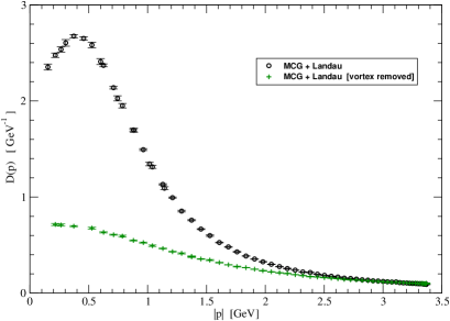
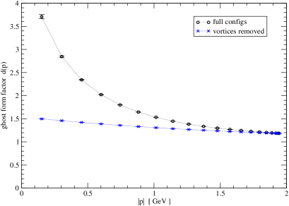
Figure 1: Left panel: The $D=3$ gluon propagator in Landau gauge after prior MCG fixing, both with and without vortices. Right panel: The same plot for the $D=3$ ghost form factor in Landau gauge.

In the left panel of Fig. 1, we first show the $D=3$ gluon propagator in Landau gauge, after prior MCG fixing. As long as vortices are not removed, the resulting propagator is virtually identical with the one obtained by fixing minimal Landau gauge directly. As can be clearly seen, the removal of vortices has little effect in the UV but clearly suppresses the propagator at intermediate and small momenta.

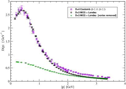
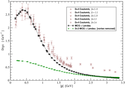
Figure 2: The equal-time gluon propagator in $D=4$ Coulomb gauge, compared to the $D=3$ gluon propagator in MCG+Landau gauge, both with and without vortices. In the left panel, we have only included $D=4$ data from two close couplings, which hides the inherent scaling violations. If more couplings are included (right panel), the scaling problems become apparent and the comparison with the $D=3$ data is less favorable.

Fig. 2 shows the equal-time gluon propagator $D_{C}(\mathbf{p})$ for Coulomb gauge in $D=4$, as obtained before removal of scaling violations. We have compared this data to the $D=3$ gluon propagator

1. directly in (minimal) Landau gauge

2. in Landau gauge after prior MCG fixing,

3. in Landau gauge after prior MCG fixing and vortex removal

(The cases a. and b. are virtually identical, and only b. is shown in Fig. 2 to make the plot less cluttered.) The confining $D=3$ MCG/Landau propagators $D_{L}(p)$ a. and b. show good agreement in the low and intermediate momentum range with the naive instantaneous $D=4$ Coulomb propagator, once the (Wilson) string tensions in the two calculations are set equal. (We took $\sqrt{\sigma}=440\,\mathrm{MeV}$ to set the scale on the momentum axis.) As expected, the non-confining Landau gauge propagator with vortices removed cannot be matched with the $D=4$ Coulomb data in any momentum range.

However, this agreement of the confining propagators must be considered spurious, since the naive $D=4$ Coulomb data is subject to severe scaling violations. In Ref. [13], these violations were thoroughly analyzed and a procedure to extract the true instantaneous propagator $D_{C}(\mathbf{p})$ in the infinite volume and continuum limit was devised. The result displays proper scaling and the correct deep ultra-violet behavior $D_{C}(\mathbf{p})\sim|\mathbf{p}|^{-1}$; it can also be fitted in the entire momentum range through the Gribov formula [13].

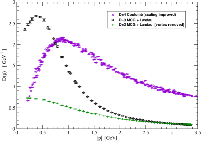
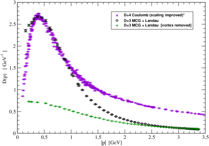
Figure 3: The equal-time gluon propagator in $D=4$ Coulomb gauge, compared to the $D=3$ gluon propagator in MCG+Landau gauge, both with and without vortices. The scaling violations in the Coulomb data are removed [13] to exhibit the true continuum result. In the left panel, the (Wilson) string tension of the $D=3$ and $D=4$ calculations are matched, while the right panel has $\sigma_{3D}\approx 6.2\,\sigma_{4D}$. (For simplicity, we have scaled $\sigma_{4D}$ and left $\sigma_{3D}$ at the standard value.)

As can be seen from the left panel in Fig. 3, the improved static Coulomb propagator $D_{C}(\mathbf{p})$ differs considerably from the naive result, so that the spurious agreement with the confining $D=3$ ensembles is destroyed. In particular, the deviation between the strong $1/p^{2}$ decay of the $D=3$ propagator and the slow $1/|\mathbf{p}|$ decay of $D_{C}(\mathbf{p})$ is now much more apparent. Qualitative agreement in the phenomenologically important momentum range around $1\,\mathrm{GeV}$ can only be reached if the $D=3$ momentum is scaled with a factor $\sim 2.5$ as compared to the $D=4$ case (see right panel in fig. 3). This in turn would mean that the scale parameter $\mu$ in the initial wave functional eq. (1) must be altered by the same factor and the $D=3$ string tension would no longer match the $D=4$ result. The best agreement is thus obtained if $\sigma_{3D}\approx 6.2\,\sigma_{4D}$, corresponding to $\mu\approx 7\,\mathrm{GeV}$.

The vortex-removed ensemble d. leads to a gluon propagator which is incompatible with the $D=4$ Coulomb result in any momentum range, even if the restrictions on the parameter $\mu$ are relaxed. This shows that the percolating center vortex content is not only indispensable for the confining properties of the Wilson loop, but also for the qualitative behavior of the gluon propagator at intermediate momenta.

As stated above, a better approximation of the correct vacuum wave functional is given by eq. (3). Indeed, either by inspecting Fig. 3 or on simple dimensional arguments, it should be clear that one should rather compare the $D=4$ static Coulomb propagator $D_{C}(\mathbf{p})$ with $p\,D_{L}(p)$ [14], which on the other hand will mimic the somewhat less crude approximation of the vacuum wave functional:

$$\Psi[\mathbf{A}]={\cal N}\exp\left(-\frac{1}{2}\int d^{3}xF_{ij}(\mathbf{x})\frac{1}{\sqrt{-\nabla^{2}}}F_{ij}(\mathbf{x})\right)\hskip 2.84544pt,$$ (11)

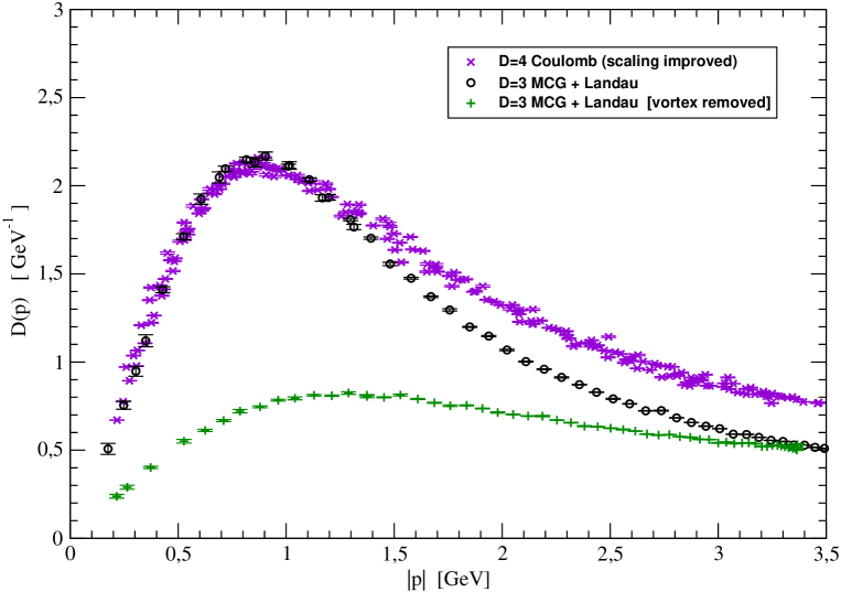
Figure 4: The gluon static propagator in $D=4$ Coulomb gauge, compared to the approximation $p\,D_{L}(p)$ of eq. (11) in $D=3$ MCG+Landau gauge.

The data basically coincide when tuning $\sigma_{3D}\approx 1.49\,\sigma_{4D}$, as can be seen in fig. 4. Such good agreement in the direction of the wave functional given in eq. (3) definitely deserves further investigation.

3.3 The ghost form factor

Although large volume simulations performed in a setup similar to ours clearly show a decoupling behavior also for the Landau ghost in $D=3$ [28], for the momenta available in our simulations this regime still has not kicked in, so that eq. (1) might still be considered a valid approximation in the following. Future simulations closer to the thermodynamic/continuum limit will however explicitely have to deal with eq. (3) or at least eq. (11), since the simple dimensional argument leading for the static gluon to the comparison in fig. 4 cannot obviously be applied to the Faddeev-Popov operator.

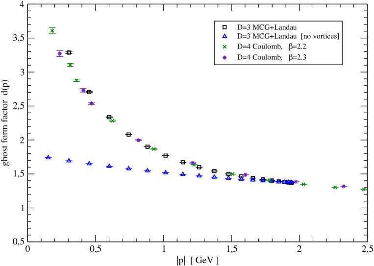
Figure 5: The ghost form factor in $D=4$ Coulomb gauge, compared to the same quantity in $D=3$ MCG+Landau gauge. The $D=4$ data is from a $32^{4}$ lattice at $\beta=2.2$ and $\beta=2.3$, while the $D=3$ data was obtained on $40^{3}$ lattices with $\beta=3.5$.

The right panel of figure 1 shows the dimensionless ghost form factor (9) as obtained from $D=3$ Landau gauge with prior MCG fixing. Without vortex removal, the result is virtually identical to the direct Landau gauge fixing, and a power law behavior of the form

$$d(p)\sim p^{-2\kappa}\,\qquad\qquad\kappa=0.23(1)$$ (12)

can be fitted. This agrees well with the infrared exponent of $D=4$ Coulomb gauge [10], which is not subject to scaling violations. Fig. 5 compares the ghost form factors in $D=3$ Landau gauge and $D=4$ Coulomb gauge quantitatively; as expected from the matching IR exponent, the comparison is fairly good. In the UV, the $d(p)$ approaches $1$ in both $D=3$ and $D=4$, so the qualitative agreement is also good in this regime. (A closer comparison of possible anomalous dimensions in the sub-leading terms is beyond our current numerical precision.)

It should be noted that the power-like behavior eq. (12) is conformally invariant, i.e. the exponent $\kappa$ is not affected by any rescaling of the momenta or string tension. This allows to maintain the good agreement of the ghost form factor, while relaxing the condition on $\mu$ to make the gluon propagators match (approximately). With the higher value of $\mu$ and the $3D$ string tension, it is therefore possible to reproduce at least qualitatively both the gluon and ghost form factor from the wave functional eq. (1), at least in the intermediate momentum range.

From the right panel in Fig. 1, it is also seen that the vortex-removed ghost form factor in $D=3$ is virtually flat ($\kappa<0.05$) so that it cannot be matched even qualitatively to the $D=4$ Coulomb result. In particular, it seems impossible to satisfy the horizon condition $d(0)^{-1}=0$ once center vortices are removed. This is, of course, expected since vortices live on the Gribov horizon and are thus indispensable to maintain enough near-zero modes of the Faddeev-Popov operator to produce the diverging ghost form factor. A similar conclusion was also reached in Ref. [6] from the direct study of the low-lying Faddeev-Popov spectrum.

4 Conclusion and outlook

In this paper we have investigated the properties of the static propagators of the Hamiltonian approach in Coulomb gauge, assuming the wave functional eq. (1), which shows strict confinement, as an approximation of the low energy limit of the true Yang-Mills vacuum wave functional. The calculation of expectation values of observables in the $D=3+1$ Hamiltonian approach in Coulomb gauge in this state requires and ordinary $D=3$ lattice simulation in Landau gauge. Adjusting the free scale $\mu$ of the state eq. (1) yields propagators which in a low to intermediate momentum regime (up to about $1~{}\mathrm{GeV}$) reproduce quite well the exact lattice propagators of the $D=3+1$ Coulomb gauge, which also agree qualitatively with propagators obtained in the variational approach to continuum Yang-Mills theory in Coulomb gauge. An even better agreement should be obtained by employing the wave functional given in eq. (3), (11), as Fig. 4 shows.

The propagators drastically change in the infra-red when the magnetic center vortices occurring with the weight $|\Psi[\mathbf{A}]|^{2}$ in the wave functional are removed by the method of Ref. [30]. In particular, the ghost form factor loses its infrared singularity and the horizon condition is no longer satisfied. These results indicate that there is no need to include additional explicit center vortex degrees of freedom in the trial wave wave functional of the variational approach, as was proposed recently [34].

References

- [1] For lattice evidence for the center vortex picture of confinement see: L. DelDebbio, M. Faber, J. Greensite and S. Olejnik, Phys. Ref. D55, 2298 (1997); K. Langfeld, H. Reinhardt and O. Tennert, Phys. Lett. B419, 316, (1998); M. Engelhardt, K. Langfeld, H. Reinhardt and O. Tennert, Phys. Rev. D61, 054504 (2000); J. Greensite, Prog. Part. Nucl. Phys. 51, 1 (2003)
- [2] For lattice evidence for the dual super-conductor picture of confinement see A.S. Kronfeld, G. Schierholz and U.-J. Wiese, Nucl. Phys. B198 (1987) 516; T. Suzuki, I. Yotsuyanagi, Phys. Ref. D42 (1990) 4257; S. Hoki et al. Phys. Lett. B272 (1991) 326; G. Bali, Ch. Schlichter, K. Schilling, Prog. Theor. Phys. Suppl. 131 (1998) 645 and Ref. therein.
- [3] Y. Nambu, Phys. Rev. D 10, 4262 (1974); S. Mandelstam, Phys. Lett. B 53, 476 (1975); G. Parisi, Phys. Rev. D 11, 970 (1975); Z. F. Ezawa and H. C. Tze, Nucl. Phys. B 100, 1 (1975); R. Brout, F. Englert and W. Fischler, Phys. Rev. Lett. 36, 649 (1976); F. Englert and P. Windey, Nucl. Phys. B 135, 529 (1978); G. ’t Hooft, Nucl. Phys. B 190, 455 (1981), Phys. Scr. 25 (1982) 133
- [4] G. ’t , Nucl. Phys. B 138, 1 (1978); G. Mack and V. B. Petkova, Annals Phys. 123, 442 (1979); G. Mack, Phys. Rev. Lett. 45, 1378 (1980); G. Mack and V. B. Petkova, Annals Phys. 125, 117 (1980); G. Mack, G. Mack and E. Pietarinen, Nucl. Phys. B 205, 141 (1982); Y. Aharonov, A. Casher and S. Yankielowicz, Nucl. Phys. B 146, 256 (1978); J. M. Cornwall, Nucl. Phys. B 157, 392 (1979); H. B. Nielsen and P. Olesen, Nucl. Phys. B 160, 380 (1979); J. Ambjorn and P. Olesen, Nucl. Phys. B 170, 60 (1980); E.T. Tomboulis, Physi. Rev. D 23, 2371 (1981)
- [5] J. Greensite and S. Olejnik, Phys. Rev. D67, 094503 (2003) [arXiv:hep-lat/0302018].
- [6] J. Greensite, S. Olejnik and D. Zwanziger, JHEP 0505, 070 (2005) [arXiv:hep-lat/0407032].
- [7] H. Reinhardt, Phys. Rev. Lett. 101, 061602 (2008) [arXiv:0803.0504 [hep-th]].
- [8] D. Zwanziger, Phys. Rev. Lett. 90, 102001 (2003) [arXiv:hep-lat/0209105].
- [9] K. Langfeld and L. Moyaerts, Phys. Rev. D70 (2004) 074507 [arXiv:hep-lat/0406024].
- [10] M. Quandt, G. Burgio, S. Chimchinda and H. Reinhardt, PoS LAT2007, 325 (2007) [arXiv:0710.0549 [hep-lat]].
- [11] A. Voigt, M. Ilgenfritz, M. Müller-Preussker, A. Sternbeck, PoS LAT2007, 338 (2007) [arXiv:0709.4585]
- [12] A. Voigt, M. Ilgenfritz, M. Müller-Preussker, A. Sternbeck, Phys. Rev. D78 (2008) 014501. [arXiv:arXiv:0803.2307 [hep-lat]].
- [13] G. Burgio, M. Quandt and H. Reinhardt, Phys. Rev. Lett. 102 (2009) 032002.
- [14] G. Burgio, M. Quandt and H. Reinhardt, arXiv:0911.5101 [hep-lat] (2009) .
- [15] A. P. Szczepaniak and E. S. Swanson, Phys. Rev. D 65, 025012 (2002) [arXiv:hep-ph/0107078].
- [16] C. Feuchter and H. Reinhardt, Phys. Rev. D 70, 105021 (2004) [arXiv:hep-th/0408236].
- [17] C. Feuchter and H. Reinhardt, arXiv:hep-th/0402106.
- [18] H. Reinhardt and C. Feuchter, Phys. Rev. D 71, 105002 (2005) [arXiv:hep-th/0408237].
- [19] D. Epple, H. Reinhardt and W. Schleifenbaum, Phys. Rev. D 75, 045011 (2007) [arXiv:hep-th/0612241].
- [20] D. Epple, H. Reinhardt, W. Schleifenbaum and A. P. Szczepaniak, Phys. Rev. D 77, 085007 (2008) [arXiv:0712.3694 [hep-th]].
- [21] H. Reinhardt and W. Schleifenbaum, Annals Phys. 324, 735 (2009) [arXiv:0809.1764 [hep-th]].
- [22] W. Schleifenbaum, M. Leder and H. Reinhardt, Phys. Rev. D 73, 125019 (2006) [arXiv:hep-th/0605115].
- [23] H. Reinhardt and D. Epple, Phys. Rev. D76 (2007) 065015, [arXiv:0706.0175 [hep-th]] .
- [24] C. Feuchter and H. Reinhardt, Phys. Rev. D 77, 085023 (2008), [arXiv:0711.2452 [hep-th]].
- [25] M. Leder, J. Pawlowski, A. Weber and H. Reinhardt, to be published
- [26] M. Pak and H. Reinhardt, arXiv:0910.2916 [hep-th] (2009) .
- [27] J. Greensite, Nucl. Phys. B158 (1979) 469.
-
[28]
A. Cucchieri and T. Mendes,
Phys. Rev. D78 (2008) 094503 [arXiv:0804.2371] ;
A. Cucchieri and T. Mendes, Phys. Rev. Lett. 100 (2008) 241601 [arXiv:0712.3517] ;
I.L. Bogolubsky et al., PoS, LATTICE2009, (2009) 237 [arXiv:0912.2249]. - [29] J. Greensite and S. Olejnik, Phys. Rev. D 77, 065003 (2008), [arXiv:0707.2860 [hep-lat]].
- [30] P. de Forcrand and M. D’Elia, Phys. Rev. Lett. 82 (1999) 4582.
-
[31]
J. Gattnar, K. Langfeld and H. Reinhardt,
Phys. Rev. Lett. 93, 061601 (2004)
[arXiv:hep-lat/0403011]
K. Langfeld, G. Schulze and H. Reinhardt, Phys. Rev. Lett. 95, 221601 (2005) [arXiv:hep-lat/0508007]. - [32] M.J. Teper, Phys. Rev. D59 (1999) 014512.
-
[33]
I.L. Bogolubsky et al.,
Phys. Rev. D74 (2006) 034503
[arXiv:hep-lat/0511056] ;
I.L. Bogolubsky et al., Phys. Rev. D77 (2008) 014504 [arXiv:0707.3611] - [34] A. Sczcepaniak, talk given at the ECT workshop QCD Green’s functions, confinement and phenomenology, Trento, September 07–11, 2009 .
-
[35]
L. v. Smekal, R. Alkofer and A. Hauck,
Phys. Rev. Lett. 79 (1997) 3591 [arXiv:hep-ph/9705242];
C. Fischer and J. Pawlowski, Phys. Rev. D75 (2007) 025012 [arXiv:hep-th/0609009];
C. Fischer, A. Maas, J. Pawlowski, Ann. Phys. 324 (2009) [arXiv:0810.1987].