Effective Polar Potential in the Central Force Schrödinger Equation

Abstract

The angular part of the Schrödinger equation for a central potential is brought to the one -dimensional ”Schrödinger form” where one has a kinetic energy plus potential energy terms. The resulting polar potential is seen to be a family of potentials characterized by the square of the magnetic quantum number $m$. It is demonstrated that this potential can be viewed as a confining potential that attempts to confine the particle to the $xy$-plane, with a strength that increases with increasing $m$. Linking the solutions of the equation to the conventional solutions of the angular equation, i.e. the associated Legendre functions , we show that the variation in the spatial distribution of the latter for different values of the orbital angular quantum number $l$ can be viewed as being a result of ”squeezing” with different strengths by the introduced ”polar potential”.

I Introduction

The Schrödinger equation for a central potential is a ”classic ” example in undergraduate and first year graduate quantum mechanics courses (see griffithsQM , for example). It is a good exercise in the separation of variables; a good example of the conservation of angular momentum, and a starting point for treating the Hydrogen atom problem. An important concept that is introduced along with this problem is that of the ”effective radial potential”, where the central potential that appears in the radial equation - after separation of variables-acquires and additional term that depends on the total angular momentum quantum number $l$ (see below). One then has a one-dimensional Schrödinger equation with an effective potential

$$V_{eff}(r)=V(r)+\frac{\hbar^{2}}{2m}\frac{l(l+1)}{r^{2}}$$ (1)

The behavior of the radial wave function is interpreted in view of this effective potential. In particular, the new repulsive part, is interpreted as a centripetal barrier that attempts to throw the particle away from the origin, thus determining its shape for different values of $l$. The present paper analyzes the angular equation along similar lines (for the polar variable $\theta$) and demonstrate that, viewed as a one-dimensional Schrödinger equation, we can identify an effective polar potential that shapes the angular part of the solution. The aim is to give the students of quantum mechanics a ”feeling” of how the spherical harmonics, that constitute the angular part of the wave function for any radial potential, assume the distribution they have about the $z$-axis. We will identify a polar potential - more precisely, a family of polar potentials that depend on the magnetic quantum number $m$ - that squeezes the particle towards the $xy$-plane with a strength that increases with $m$. The physical picture introduced, and the intuition employed, we believe, will also provide the students with a simple prototype of the intuitive thinking that is employed by practicing physicists in understanding more complex real-world systems.

II The Solutions of the Schrödinger Equation for a Central Potential

The Schrödinger equation

$$-\frac{\hbar^{2}}{2m}\nabla^{2}\psi+V\psi=E\psi$$

separates in spherical coordinates for a central potential by writing $\psi=R(r)Y(\theta,\phi)$, and introducing the separation constant $l(l+1)$ . The resulting radial and angular equations are, respectively:

$$\frac{1}{R}\frac{d}{dr}\left(r^{2}\frac{dR}{dr}\right)-\frac{2mr^{2}}{\hbar^{2}}\left[V(r)-E\right]=l(l+1)$$ (2)

$$\frac{1}{\sin\theta}\frac{\partial}{\partial\theta}\left(\sin\theta\frac{\partial Y}{\partial\theta}\right)+\frac{1}{\sin^{2}\theta}\frac{\partial^{2}Y}{\partial\phi^{2}}=-l(l+1)Y$$ (3)

The radial equation is brought to the Schrödinger form by substituting:

$$u(r)=rR(r)$$

so equation (2) becomes:

$$-\frac{\hbar^{2}}{2m}\frac{d^{2}u}{dr^{2}}+\left\{V(r)+\frac{\hbar^{2}}{2m}\frac{l(l+1)}{r^{2}}\right\}u=Eu$$ (4)

with the term in the brackets being the effective potential we mentioned above, equation (1).

Now if we look at equation (3), the so called angular equation, we can do one more separation of variables by setting $Y(\theta,\phi)=\Theta(\theta)\Phi(\phi)$, then we will have the azimuthal angle equation,

$$\frac{d^{2}\Phi}{d\phi^{2}}+m^{2}\Phi=0$$ (5)

and the polar equation,

$$\frac{1}{\sin\theta}\frac{d}{d\theta}\left(\sin\theta\frac{d\Theta}{d\theta}\right)-\frac{m^{2}}{\sin^{2}\theta}\Theta=-l(l+1)\Theta$$ (6)

the solutions of (5) are

$$\Phi(\phi)=e^{im\phi}$$ (7)

and we require the solutions $\Phi(\phi)$ to be single valued, i.e

$$\Phi(\phi+2\pi)=\Phi(\phi)$$

which dictates that $m=0,\pm 1,\pm 2,...$. It is worth to recall that the r.h.s of (3) is the total angular momentum hermitian operator $L^{2}$ represented in spherical coordinates. In general $L^{2}$ admits integer and half integer solutions for the eigenvalue $l$, which is the result of the angular momentum commutation relations. The restriction of $l$ to integers is a consequence of restricting $m$ to integers.

Let’s go back to equation (6), and write down its famous solutions which are the associated Legendre functions griffithsQM ; boas ($N_{l}^{m}$ is a normalization constant):

$$\Theta(\theta)=N_{l}^{m}P^{m}_{l}(\cos\theta)$$ (8)

where $P^{m}_{l}$ are given by

$$P^{m}_{l}(x)=(1-x^{2})^{\frac{|m|}{2}}\left(\frac{d}{dx}\right)^{|m|}P_{l}(x)$$ (9)

where $P_{l}(x)$ are the the Legendre polynomials which are given by the Rodrigues formula griffithsQM ; boas :

$$P_{l}(x)=\frac{1}{2^{l}l!}\left(\frac{d}{dx}\right)^{l}(x^{2}-1)^{l}$$ (10)

The solutions $|P_{l}^{m}(\cos\theta)|^{2}$ represent the probability of finding the particle at a certain angle $\theta$, which means that they give the probability distribution of the particle about the $z$-axis. We will show below that we can view this distribution as being shaped by a polar potential.

III The Polar Potential

Now we can bring the polar equation (6) to the Schrödinger form, just as we did with the radial equation. Defining:

$$\Theta(\theta)=\sin^{-\frac{1}{2}}(\theta)y(\theta)$$ (11)

and multiplying by 1/2, equation (6) becomes

$$-\frac{1}{2}\frac{d^{2}y(\theta)}{d\theta^{2}}+\left\{\frac{m^{2}-\frac{1}{4}}{2\sin^{2}(\theta)}\right\}y(\theta)=Ey(\theta)$$ (12)

where $E=(1/2)(l(l+1)+1/4)$.

This equation can be thought of as a one dimensional Shrödinger equation (with $\hbar=m=1$ ) for a particle confined between $0$ and $\pi$, and satisfying the boundary conditions $y(0)=y(\pi)=0$. The term in brackets is a one dimensional potential, more precisely it is a family of potentials depending on the choice of the value of $m$. 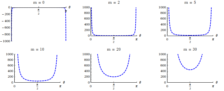These potentials are special cases of the so called Pöschl-Teller potential poschl ; flugge . To gain a closer look at the potential, we plot it for various $m$-values in Fig.1. As the figure intuitively suggests, the potential, which is infinite at the boundaries - thus banning the particle from going beyond the boundary- attempts to confine the particle about the $z$-axis, the higher $m$ is the stronger is the confining strength. For the lower $m$ values the potentials are very close to an infinite well with width $\pi$, as we increase $m$ the potential squeezes the states resulting in more confinement.

Figure 1: Graphs of the potential for several values of integer m

Let’s take a look at the solutions now. The solutions for this family of potentials can be worked out in several ways, a nice algebraic way is to use Infeld and Hull factorization method infeldHull . This family of potentials enjoys shape invariance symmetry, which can be exploited to workout the eigenvalues algebraically. Supersymmetric quantum mechanics techniques can also be used to work out the eigenstates dutt . We will not use these techniques here, rather we will work out the solutions from the solutions of the original angular equation (6). If we restrict the values of $m$ to nonnegative integers, the solutions, upon employing the transformation (11) can be written directly from the solutions of the original equation and they read

$$y_{n}^{m}(\theta)=N_{n}^{m}\sin^{\frac{1}{2}}\theta\ P_{n+m}^{m}(\cos\theta)$$ (13)

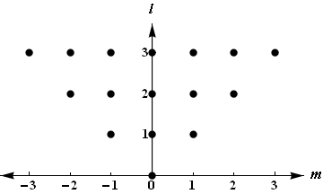
where $P_{n+m}^{m}$ are, again, the associate Legendre functions. These solutions are for nonnegative $m$, those for negative $m$ are - as is well-known griffithsQM ; boas - directly proportional to these solutions. So, without loss of generality, we will restrict ourselves to nonnegative $m$ values. In the original equation (6), the solutions are conventionally labeled by a pair of numbers ($m$,$l$) and subject to the condition $m\leq l$. The pairs ($m$,$l$) constitute a lattice as shown in Fig.2. In the conventional interpretation of the solutions of (6) the number $l$ is associated with the angular momentum, so the usual way to look at the grid of solutions is to fix the angular momentum by fixing $l$ and then changing $m$, so all the solutions with different $m$’s and same $l$ are degenerate and correspond to the same angular momentum. This amounts to moving right (or left) on the grid. But what we are doing here is different, we are fixing $m$ and looking at the solutions of a one-dimensional potential at a fixed $m$ value. When we fix the value of $m$ to a specific integer we get all the solutions for that one dimensional potential. As one can see, the first eigenstate for $m=1$ is at $l=1$, but it still corresponds to the ground state of $m=1$ potential, which will be labeled as $n=0$, where $n$ is the quantum number which labels the states of a fixed $m$ potential. The same thing happens with all other $m$-values, thus we are moving up the grid shown in Fig.2. It is always the case that the ground state of a fixed $m$ potential coincides with a $l=m$, therefore, the relation between $l$ and $n$ is $l=m+n$. Consequently, the eigenergies can now be written down directly from those of equation (12); they read:

$$E_{n}^{m}=\frac{1}{2}(n+m+\frac{1}{2})^{2}$$ (14)

Here, higher values of $n$, i.e. excited states correspond to higher values of the kinetic energy of the confined particle. That this corresponds to higher $l$-values -in the conventional view- is natural, as higher kinetic energies mean higher angular momenta.

Figure 2: $l$ and $m$ lattice

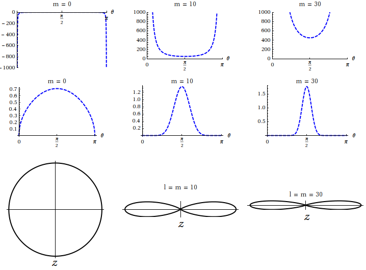
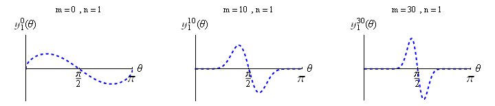
Now, we show how to relate the behavior of the potential to that of the eigenenergies, eigenstates and the original associate Legendre functions. Let’s look again at the graphs of the potential for several $m$ in Fig.(1). Here we note that as $m$ increases the bottom of the potential is shifted up, and this is responsible for increasing the ground state energy with increasing $m$. The second observation here is that as one goes for higher values of $m$, the potential tends to confine the particle closer to the mid point of the potential $\left(\theta=\frac{\pi}{2}\right)$, which means confining the particle closer to the $xy$-plane. This is confirmed by looking at the behavior of the ground states for several $m$. In Fig. (3) we plot the ground states for various values of $m$ just below the corresponding potential. It is clear that as $m$ increases the ground state gets squeezed closer to middle of the box, giving rise to more confinement of the particle. The last line in Fig.(3) shows the corresponding associated Legendre functions which are related to the eigenfunctions through the transformation (11). It is quite obvious that the particle is more likely to be found near the $xy-$plane as $m$ increases. Since higher $m$ means higher angular momentum, this squeezing of the states towards the $xy-$plane can be explained semi-classically in terms of the increase of the moment of inertia of the particle about the $z-$axis. Finally, while the examples we have considered above are for the ground states only, the same arguments apply equally well to the excited states. Fig. (4) shows the first excited states; $n=1$, for three $m$-values. It is clear that as one goes up in $m$, the particle gets more squeezed towards the $xy$-plane.

Figure 3: The first row shows the potential for three values of $m$, the second row shows the ground state solutions for those potentials, the last line shows the polar plots for the Legendre functions with the argument $\cos\theta$ for the corresponding values of $m$ and $l$

In conclusion, we see that we can view the angular distribution in the wave functions of a particle in a central potential as being a result of confinement by an $m-$dependent ”effective” polar potential.

Figure 4: The first excited states for $m=0,10,30$.The excited states get more confined about $\theta=\pi/2$ as $m$ increases

References

- [1] David Griffiths. Introduction to Quantum Mechanics. Pearson Prentice Hall, second edition, 2005.
- [2] Mary Boas. Mathematical Methods in the Physical Sciences. Wiley, third edition, 2006.
- [3] G. Pöschl and E. Teller. The factorization method. Z. Phys., 83:143–151, 1933.
- [4] S.Flugge. Practical Quantum Mwchanics I. Springer-Verlag, 1970.
- [5] L. Infeld and T. E. Hull. The factorization method. Rev. Mod. Phys., 23(1):21–68, Jan 1951.
- [6] Ranabir Dutt, Avinash Khare, and Uday P. Sukhatme. Am.J. Phys., 56(2):163–168, 1988.