Cross Section Evaluation by Spinor Integration II: The massive case in 4D

Abstract:

In this paper, we continue our study of calculating the cross section by the spinor method, i.e., performing the phase space integration using the spinor method. We have focused on the case where the physical momenta are massive and in pure 4D. We established the framework of such a new method and presented several examples, including two real progresses: $Z^{0}\to l^{+}l^{-}H$ and $q\overline{q}\to f\overline{f}H^{0}$.

1 Introduction

In the Tevatron collider and the LHC, multiple final states are observed frequently. In order to check the standard model and looking forward to finding new physics beyond the standard model [1, 2, 3, 4], we need to explore the problem of how to calculate the cross section efficiently and conveniently. In the past, the cross section is evaluated in the 3-dimensional momentum space [5, 6] and people have developed quite mature numerical techniques. For the applications of programs Madgraph, Pythia, AlpGen and Sherpa, the reader can check references, for example, [7].

On the other hand, enormous progress have been made in the evaluation of one-loop amplitudes [2]. One of such progress is the unitarity cut method originally proposed in [8, 9]. With the twistor program initiated by Witten [10], the double cut phase space integration has been reduced to algebraic manipulation through the holomorphic anomily [11, 12, 13, 14]. Inspired by this simplification, in our first paper [15], we have explored how to apply the spinor integration method to the evaluation of the cross section for massless case. There are some obvious advantages comparing with the momentum integration method. First, the three-dimension momentum space integration can be reduced to just one-dimensional integration and furthermore for the massless case, the integration region is just $[0,1]$. Secondly, in the calculation, every step is manifestly Lorentz invariant, thus we obtain compact analytic expressions.

Continuing our study for the massless case, in this paper we focus on the massive case. We will see that if all the mass is set to zero, the massless case will be reproduced. Different from the massless case, the integration variable $L$ is no longer a null momentum. So we can’t apply the spinor method directly. However this problem have been solved in the unitarity cut method [16, 17]. More accurately, we can write

$$\int d^{4}L=\int dz\int d^{4}\ell\delta^{+}(\ell^{2})(2\ell\cdot K);\quad L=\ell+zK,$$ (1)

where $K$ is a fixed vector and $z$ is a real number. Through this decomposition, we establish the general framework for massive case by the spinor method.

In our first paper, we have emphasized the advantages of using the spinor method [15]. In the massive case, the constrained three-dimensional momentum space integration still can be reduced to an one-dimensional integration, plus possible Feynman integrations. In every step, we get a scalar type of integrations, which are Lorentz invariant. Furthermore, the integration region can be written directly. Though it’s not simply $[0,1]$ like the massless case, it’s only the simple functions of mass and energy.

The outline of this paper is as follows. In section 2, we first briefly review the 4D unitarity cut method. Then we take the Faddeev-Popov trick to establish the general framework.

In section 3, we apply our method to the pure phase space integration for two, three and four out-going particles as well as some simple examples to demonstrate the main idea and feature. These are the basis for practical and more complicated applications.

In section 4, we calculate two practical examples and summarize some experience of performing the integrations.

A summary of our results with some comments is given in section 5.

2 Framework to use spinor method

In this section, we will setup the spinor integration method for massive particles in 4D. Then we apply this method to the phase space integration where the integration region (i.e, the $\int dx$) of one dimensionless parameter is determined by the kinematical discussion. This region corresponds to the boundary of the whole phase space of outgoing momenta. One important difference, compared to the massless case, is that the integration region will be functions of masses of outgoing particles.

2.1 The spinor integration method for massive cuts

Here, we briefly review the spinor integration method for massive cuts (or sometimes called the “unitarity cut method”) [16, 17, 18]. The Lorentz-invariant phase space (LIPS) of a massive double cut is defined by inserting two $\delta$-functions representing the cut conditions:

$$I=\int d^{4}~{}\widetilde{\ell}\delta^{+}(\widetilde{\ell}^{2}-m_{1}^{2})\delta((K-\widetilde{\ell})^{2}-m_{2}^{2}),$$ (2)

where $\widetilde{\ell}$ is the internal loop momentum and $K$ the total momentum through the unitarity cut. Because $\widetilde{\ell}$ is a massive momentum, to use spinor integration method we need decompose it as

$$\widetilde{\ell}=\ell+zK,\quad\ell^{2}=0;\quad\int d^{4}\widetilde{\ell}=\int dzd^{4}\ell~{}\delta^{+}(\ell^{2})(2\ell\cdot K).$$ (3)

where $\ell$ is a null 4-momentum, and can be expressed with spinor variables as

$$\ell=tP_{\lambda\widetilde{\lambda}},\quad P_{\lambda\widetilde{\lambda}}=\lambda\widetilde{\lambda};\quad\int d^{4}\ell~{}\delta^{+}(\ell^{2})=\int\left\langle\lambda~{}\lambda\right\rangle\left[\widetilde{\lambda}~{}\widetilde{\lambda}\right]\int tdt.$$ (4)

Under this decomposition Eq.(2) becomes

$$I = \int dzd^{4}\ell\delta^{+}(\ell^{2})(2\ell\cdot K)\delta^{+}(z^{2}K^{2}+2zK\cdot\ell-m_{1}^{2})\delta^{+}((1-2z)K^{2}-2K\cdot\ell+m_{1}^{2}-m_{2}^{2})$$ (5)

$$= \int dz~{}((1-2z)K^{2}+m_{1}^{2}-m_{2}^{2})\delta^{+}(z(1-z)K^{2}+z(m_{1}^{2}-m_{2}^{2})-m_{1}^{2})$$

$$\int\left\langle\lambda~{}\lambda\right\rangle\left[\widetilde{\lambda}~{}\widetilde{\lambda}\right]{(1-2z)K^{2}+m_{1}^{2}-m_{2}^{2}\over\left\langle\lambda|K|\widetilde{\lambda}\right]^{2}},\quad t={(1-2z)K^{2}+m_{1}^{2}-m_{2}^{2}\over\left\langle\lambda|K|\widetilde{\lambda}\right]}.$$

In the first line of the result it depends only on the variable $z$, so we can use the $\delta$-function to eliminate $z$ as follows

$$z_{\pm}={(K^{2}+m_{1}^{2}-m_{2}^{2})\pm\sqrt{\Delta[K,m_{1},m_{2}]}\over 2K^{2}}~{},$$ (6)

where we have defined

$$\Delta[K,m_{1},m_{2}]=(K^{2}-m_{1}^{2}-m_{2}^{2})^{2}-4m_{1}^{2}m_{2}^{2}~{}.$$ (7)

Between the two solutions of $z$, only one should be taken. To see that, we make a kinematical analysis. Choose a center-of-mass frame such that

$$K=(E>0,0,0,0),\quad\widetilde{\ell}=(a,b,0,0),\quad K-\widetilde{\ell}=(E-a,-b,0,0).$$

The mass-shell conditions require $a^{2}-b^{2}=m_{1}^{2}$ and $(E-a)^{2}-b^{2}=m_{2}^{2}$, so $a={(E^{2}+m_{1}^{2}-m_{2}^{2})/2E}$. In the decomposition $\widetilde{\ell}=\ell+zK$, because the positive light cone with $\delta^{+}(\ell)$ have been chosen, we can write

$$\ell=(|b|,b,0,0),\quad\widetilde{\ell}=(|b|+zE,b,0,0)$$

Then $|b|+zE=a$. This means that only $z_{-}$ is retained. In the following of this paper, we always refer to $z$ as $z_{-}$ , if it’s not explicitly illustrated.

Then Eq.(5) becomes

$$I=\int\left\langle\lambda~{}\lambda\right\rangle\left[\widetilde{\lambda}~{}\widetilde{\lambda}\right]{(1-2z)K^{2}+m_{1}^{2}-m_{2}^{2}\over\left\langle\lambda|K|\widetilde{\lambda}\right]^{2}},\quad t={(1-2z)K^{2}+m_{1}^{2}-m_{2}^{2}\over\left\langle\lambda|K|\widetilde{\lambda}\right]}.$$ (8)

Eq.(8) is our final form for the spinor integration with massive double cuts. For convenience we define

$$z[K,m_{1},m_{2}]={\alpha[K,m_{1};m_{2}]-\beta[K;m_{1},m_{2}]\over 2},\quad t={\beta K^{2}\over\left\langle\lambda|K|\widetilde{\lambda}\right]},$$ (9)

where

$$\alpha[K,m_{1};m_{2}]\equiv{K^{2}+m_{1}^{2}-m_{2}^{2}\over K^{2}},\quad\beta[K;m_{1},m_{2}]\equiv{\sqrt{\Delta[K,m_{1},m_{2}]}\over K^{2}}.~{}~{}~{}~{}~{}$$ (10)

Notice that when $m_{1}=m_{2}=0$ we have $\alpha=\beta=1$, thus reproducing the massless case. Finally the original $\widetilde{\ell}$ can be parameterized as

$$\widetilde{\ell}=tP_{\lambda\widetilde{\lambda}}+zK={K^{2}\over\left\langle\lambda|K|\widetilde{\lambda}\right]}\left[\beta\left(P_{\lambda\widetilde{\lambda}}-{K\cdot P_{\lambda\widetilde{\lambda}}\over K^{2}}K\right)+\alpha{K\cdot P_{\lambda\widetilde{\lambda}}\over K^{2}}K\right].$$ (11)

2.2 Spinor integration method for the physical phase space integration

Now, we explore how to apply the spinor integration method for massive cuts to the phase space integration. Just like the massless case, when there are only two outgoing particles, spinor integration method can be applied directly without any modification. To see explicitly, just write the phase space of the cross section:

$$I_{2} = \prod_{f=1,2}\int{d^{4}L_{f}\over(2\pi)^{3}}\delta^{+}(L_{f}^{2}-m_{i}^{2})(2\pi)^{4}\delta^{4}(K-\sum_{f=1,2}L_{f})$$ (12)

$$\sim \int d^{4}L_{1}\delta^{+}(L_{1}^{2}-m_{1}^{2})\delta^{+}((K-L_{1})^{2}-m_{2}^{2}),$$

which is exactly the same (namely the show-up of two $\delta$-functions) as the spinor integration method given in Eq.(2).

Thing will be different when $n=3$, where the physical phase space is given by:

$$I_{3} = \prod_{i=1}^{3}\int{d^{4}L_{i}\over(2\pi)^{3}}\delta^{+}(L_{i}^{2}-m_{i}^{2})(2\pi)^{4}\delta^{4}(K-\sum L_{i})f(L_{1},L_{2},L_{3})$$ (13)

$$= \int{d^{4}L_{3}\over(2\pi)^{3}}\delta^{+}(L_{3}^{2}-m_{3}^{2})\int{d^{4}L_{2}\over(2\pi)^{2}}\delta^{+}(L_{2}^{2}-m_{2}^{2})\delta^{+}((K-L_{3}-L_{2})^{2}-m_{1}^{2})f(L_{2},L_{3})$$

$$= \int{d^{4}L_{3}\over(2\pi)^{3}}\delta^{+}(L_{3}^{2}-m_{3}^{2})\widetilde{f}(L_{3}).$$

The problem we meet here is just the same as the massless case. The integration over $L_{2}$ with two $\delta$-functions can be performed by the spinor integration method. However, there is only one $\delta$-function in the integration over $L_{3}$. In order to apply the spinor method recursively and continuously, we need insert one more $\delta$-function like the Faddeev-Popov method.

Similarly to the massless case [15], we consider the following integration

$$I_{x} \equiv \int dx\delta((xK-L_{3})^{2}-m_{3}^{2})=\int dx\delta(x^{2}K^{2}-x(2K\cdot L_{3})+L_{3}^{2}-m_{3}^{2}),$$

where the $\delta$-function has two solutions

$$x_{i} = {(2K\cdot L_{3})\pm\sqrt{(2K\cdot L_{3})^{2}-4K^{2}(L_{3}^{2}-m_{3}^{2})}\over 2K^{2}}~{}.$$ (14)

Using the on-shell condition $L_{3}^{2}=m_{3}^{2}$, it reduces to

$$x_{-}=0,~{}~{}~{}~{}x_{+}={2K\cdot L_{3}\over K^{2}}~{}.$$ (15)

We find that $x_{-}=0$ is always a root. However, when $x=0$, we have $\delta(L_{3}^{2}-m_{3}^{2})$ which does not give an independent $\delta$-function. So $x_{-}=0$ should be excluded from our consideration. For another root $x_{+}$, from $(K-L_{3})^{2}=K^{2}+m_{3}^{2}-2K\cdot L_{3}\geq(m_{1}+m_{2})^{2}$, we have

$$2K\cdot L_{3}\leq K^{2}+m_{3}^{2}-(m_{1}+m_{2})^{2},$$ (16)

which gives the upper bound of $x_{+}$. For the lower bound, considering the center-of-mass frame where $K=(E,0,0,0)$, $L_{3}=(E_{3},p,0,0)$ with $E_{3}^{2}-p^{2}=m_{3}^{2}$, we have $2K\cdot L_{3}\geq 2Em_{3}$, i.e., $(2K\cdot L_{3})^{2}\geq 4K^{2}m_{3}^{2}$.

Putting all consideration together we have

$$I_{x} \equiv \int_{x_{0}}^{x_{1}}dx\delta((xK-L_{3})^{2}-m_{3}^{2})=\int_{x_{0}}^{x_{1}}dx{\delta(x-x_{+})\over|2x_{+}K^{2}-(2K\cdot L_{3})|}$$ (17)

$$= {1\over|\sqrt{(2K\cdot L_{3})^{2}-4K^{2}(L_{3}^{2}-m_{3}^{2})}|},~{}~{}~{}~{}$$

where

$$x_{0}[K,m_{3}]\equiv\sqrt{4m_{3}^{2}\over K^{2}},~{}~{}~{}~{}~{}x_{1}[K,m_{3};m_{t}]\equiv{K^{2}+m_{3}^{2}-m_{t}^{2}\over K^{2}}=\sqrt{x_{0}[K,m_{3}]^{2}+\Lambda[K;m_{3},m_{t}]^{2}}~{},$$ (18)

where $\Lambda[K;m_{3},m_{t}]={\sqrt{\Delta[K,m_{3},m_{t}]}/K^{2}}$ with $m_{t}=m_{1}+m_{2}$. Using $K^{2}\geq(m_{1}+m_{2}+m_{3})^{2}$, it is easy to see that $\Lambda[K;m_{3},m_{t}]^{2}\geq 0$ and thus $x_{1}\geq x_{0}$.

Now Eq.(13) can be written as

$$I_{3} = {1\over(2\pi)^{3}}\int d^{4}L_{3}\delta^{+}(L_{3}^{2}-m_{3}^{2}){|\sqrt{(2K\cdot L_{3})^{2}-4K^{2}(L_{3}^{2}-m_{3}^{2})}|}\int_{x_{0}}^{x_{1}}dx\delta((xK-L_{3})^{2}-m_{3}^{2})\widetilde{f}(L_{3}).$$

Decomposing $L_{3}=\ell+zK$ with $\ell^{2}=0$, then

$$I_{3} = {1\over(2\pi)^{3}}\int dzd^{4}\ell\delta^{+}(\ell^{2})(2\ell\cdot K)\delta^{+}(z^{2}K^{2}+2zK\cdot\ell-m_{3}^{2}){(2L_{3}\cdot K)}\int_{x_{0}}^{x_{1}}dx\delta^{+}({x^{2}K^{2}-2xK\cdot L_{3}})\widetilde{f}(\ell)$$ (19)

$$= {1\over(2\pi)^{3}}\int_{x_{0}}^{x_{1}}dx{xK^{2}}\int dz(x-2z)K^{2}\delta^{+}(z(x-z)K^{2}-m_{3}^{2})$$

$$\hphantom{{1\over(2\pi)^{3}}\int_{x_{0}}^{x_{1}}dx}\times\int d^{4}\ell\delta^{+}(\ell^{2})\delta^{+}(x(x-2z)K^{2}-2xK\cdot\ell)\widetilde{f}(\ell).$$

One by-product of the above procedure is

$$2K\cdot L_{3}=xK^{2}~{}.~{}~{}$$ (20)

By solving the $\delta$-function $\delta^{+}(z(x-z)K^{2}-m_{3}^{2})$ and the similar kinematical discussion as in Section 2.1, we get

$$z = {xK^{2}-\sqrt{K^{2}(x^{2}K^{2}-4m_{3}^{2})}\over 2K^{2}}={x\over 2}-{\sqrt{x^{2}-x_{0}^{2}}\over 2},~{}~{}~{}~{}x-2z=\sqrt{x^{2}-x_{0}^{2}}~{}.$$ (21)

Continue the evaluation as

$$I_{3} = {c\over(2\pi)^{3}}\int_{x_{0}}^{x_{1}}dx{xK^{2}}\int\left\langle\lambda|d\lambda\right\rangle\left[\widetilde{\lambda}|d\widetilde{\lambda}\right]\int tdt\delta^{+}(x(x-2z)K^{2}-xt\left\langle\lambda|K|\widetilde{\lambda}\right])\widetilde{f}(\lambda,\widetilde{\lambda},t)$$ (22)

$$= {c\over(2\pi)^{3}}\int_{x_{0}}^{x_{1}}dx{xK^{2}}\int\left\langle\lambda|d\lambda\right\rangle\left[\widetilde{\lambda}|d\widetilde{\lambda}\right]{(x-2z)K^{2}\over x\left\langle\lambda|K|\widetilde{\lambda}\right]^{2}}\widetilde{f}(\lambda,\widetilde{\lambda},t),~{}~{}~{}~{}t={(x-2z)K^{2}\over\left\langle\lambda|K|\widetilde{\lambda}\right]}$$

$$= {c\over(2\pi)^{3}}\int_{x_{0}}^{x_{1}}dx(K^{2})^{2}\sqrt{x^{2}-x_{0}^{2}}\int\left\langle\lambda|d\lambda\right\rangle\left[\widetilde{\lambda}|d\widetilde{\lambda}\right]{\widetilde{f}(\lambda,\widetilde{\lambda},t)\over\left\langle\lambda|K|\widetilde{\lambda}\right]^{2}},~{}~{}~{}~{}t={K^{2}\sqrt{x^{2}-x_{0}^{2}}\over\left\langle\lambda|K|\widetilde{\lambda}\right]},$$

where $c=\pi/2$ is related to the Jacobi of changing integration variables and the way we have taken the residues.

Finally we arrive

$$I_{3} = \int{d^{4}L_{3}\over(2\pi)^{3}}\delta^{+}(L_{3}^{2}-m_{3}^{2})\widetilde{f}(L_{3})$$ (23)

$$= {\pi\over 2(2\pi)^{3}}\int_{x_{0}}^{x_{1}}dx(K^{2})^{2}\sqrt{x^{2}-x_{0}^{2}}\int\left\langle\lambda|d\lambda\right\rangle\left[\widetilde{\lambda}|d\widetilde{\lambda}\right]{\widetilde{f}(\lambda,\widetilde{\lambda},t)\over\left\langle\lambda|K|\widetilde{\lambda}\right]^{2}},~{}~{}~{}~{}t={K^{2}\sqrt{x^{2}-x_{0}^{2}}\over\left\langle\lambda|K|\widetilde{\lambda}\right]}~{}~{}~{}\smash{\hbox to0.0pt{\raise 4.30554pt\hbox{\tiny[I3-form]}\hss}}$$

This is our key setup in this paper. Notice that when $m_{1}=m_{2}=m_{3}=0$, $x_{0}=0$, so Eq. (23) reduces to

$$I_{3} = \int{d^{4}L_{3}\over(2\pi)^{3}}\delta^{+}(L_{3}^{2})\widetilde{f}(L_{3})$$ (24)

$$= {\pi\over 2(2\pi)^{3}}\int_{0}^{1}dx(K^{2})^{2}x\int\left\langle\lambda|d\lambda\right\rangle\left[\widetilde{\lambda}|d\widetilde{\lambda}\right]{\widetilde{f}(\lambda,\widetilde{\lambda},t)\over\left\langle\lambda|K|\widetilde{\lambda}\right]^{2}},~{}~{}~{}~{}t={K^{2}x\over\left\langle\lambda|K|\widetilde{\lambda}\right]}.$$

which is the familiar massless case presented in [15].

In the end, let us give a remark. The integration region of $x\in[x_{0},x_{1}]$ depends on the dynamical momentum $K$ as well as mass parameters $m_{3}$ and $m_{total}$. Because this, the roles of $m_{3}$ and $m_{total}$ are not obviously symmetric. If we define

$$x=\sqrt{x_{0}^{2}+\Lambda^{2}u^{2}}~{},$$ (25)

the integration region of $u$ will be $u\in[0,1]$ which does not depend on external momenta and masses anymore. Under this transformation we have

$$I_{3} = {\pi\over 2(2\pi)^{3}}\int_{0}^{1}du(K^{2})^{2}{\Lambda^{3}u^{2}\over\sqrt{x_{0}^{2}+\Lambda^{2}u^{2}}}\int\left\langle\lambda|d\lambda\right\rangle\left[\widetilde{\lambda}|d\widetilde{\lambda}\right]{\widetilde{f}(\lambda,\widetilde{\lambda},t)\over\left\langle\lambda|K|\widetilde{\lambda}\right]^{2}},~{}~{}~{}~{}t={K^{2}\Lambda u\over\left\langle\lambda|K|\widetilde{\lambda}\right]}.~{}~{}~{}$$ (26)

and

$$L_{3} = {K^{2}\Lambda u\over\left\langle\lambda|K|\widetilde{\lambda}\right]}\lambda\widetilde{\lambda}+\left({\sqrt{x_{0}^{2}+\Lambda^{2}u^{2}}\over 2}-{\Lambda u\over 2}\right)K.$$ (27)

This transformation will become even simpler when $m_{3}=0$ where we get a just linear transformation $x=\Lambda u$. Although Eq. (26) may look simpler, however by some calculations we find that Eq. (26) is, in general, not better than Eq. (23) and readers can use anyone they like. In the later part of this paper, we will use the form of Eq. (23).

3 Simple examples

In this section, we present some very simple examples to demonstrate our method, especially the integration region of $x$. We denote the physical phase space integration of $n$ outgoing particles as $I_{n}^{s\,\mathrm{or}\,m}(f;K)$, where $s$ stands for the spinor method and $m$ the momentum method. The $K$ is the sum of momenta of these $n$ particles and $f$ is a general function.

3.1 The pure phase space integration with two outgoing particles

This integral can be performed directly by the spinor method as we have analyzed in last section.

Spinor integration method: The integration is given by

$$I_{2}^{s}(1;K) = \int{d^{4}L_{2}\over(2\pi)^{3}}{d^{4}L_{1}\over(2\pi)^{3}}\delta^{+}(L_{2}^{2}-m_{2}^{2})\delta^{+}(L_{1}^{2}-m_{1}^{2})(2\pi)^{4}\delta^{4}(K-L_{2}-L_{1})$$ (28)

$$= {1\over(2\pi)^{2}}\int d^{4}L_{1}\delta^{+}(L_{1}^{2}-m_{1}^{2})\delta^{+}((K-L_{1})^{2}-m_{2}^{2}).$$ (29)

According to Eq.(8), one gets

$$I_{2}^{s}(1;K) = {\pi\over 2(2\pi)^{2}}\int\left\langle\lambda~{}\lambda\right\rangle\left[\widetilde{\lambda}~{}\widetilde{\lambda}\right]{(1-2z)K^{2}+m_{1}^{2}-m_{2}^{2}\over\left\langle\lambda|K|\widetilde{\lambda}\right]^{2}}={1\over(2\pi)^{2}}{\pi\over 2}\beta$$ (30)

$$= {1\over 2(2\pi)^{2}}{\sqrt{(K^{2}-m_{1}^{2}-m_{2}^{2})^{2}-4m_{1}^{2}m_{2}^{2}}\over K^{2}},~{}~{}~{}~{}$$

which is obviously symmetric between $m_{1},m_{2}$.

Momentum integration method: It is given by

$$I_{2}^{m}(1;K) = \int\frac{dL_{1}^{3}}{(2\pi)^{3}2E_{1}}\frac{dL_{2}^{3}}{(2\pi)^{3}2E_{2}}(2\pi)^{4}\delta^{4}(K-L_{2}-L_{1}).$$ (31)

Taking the center-of-mass frame, where $K=(E,0,0,0)$ and $L_{1}=(E_{1},k_{1},0,0)$, yields

$$I_{2}^{m}(1;K) = {1\over(2\pi)^{2}}\int{k_{1}^{2}dk_{1}\over 2E_{2}}d\Omega\delta^{+}(E^{2}-2EE_{1}+m_{1}^{2}-m_{2}^{2})={1\over(2\pi)^{2}}{\pi\over 2}\beta.$$ (32)

3.2 The pure phase space integration with three outgoing particles

Spinor integration method: From Eq.(13) with the result $I_{2}^{s}(1;K)$ in previous subsection we have

$$I_{3}^{s}(1,K) = \int{d^{4}L_{3}\over(2\pi)^{3}}\delta^{+}(L_{3}^{2}-m_{3}^{2})I_{2}^{s}(1;K-L_{3})$$ (33)

$$= {\pi\over 2(2\pi)^{3}}\int_{x_{0}}^{x_{1}}dx(K^{2})^{2}\sqrt{x^{2}-x_{0}^{2}}\int\left\langle\lambda|d\lambda\right\rangle\left[\widetilde{\lambda}|d\widetilde{\lambda}\right]{I_{2}^{s}(1;K-L_{3})\over\left\langle\lambda|K|\widetilde{\lambda}\right]^{2}},$$ (34)

where $I_{2}^{s}(1;K-L_{3})$ depends on $(K-L_{3})^{2}$ only. But using $L_{3}^{2}-m_{3}^{2}=0$ and $(xK-L_{3})^{2}-m_{3}^{2}=0$, we can find

$$(K-L_{3})^{2} = (1-x)K^{2}+m_{3}^{2},$$ (35)

which does not depend on $\lambda,\widetilde{\lambda}$ at all. Thus

$$I_{3}^{s}(1,K) = {\pi\over 2(2\pi)^{3}}\int_{x_{0}}^{x_{1}}dxK^{2}\sqrt{x^{2}-x_{0}^{2}}~{}I_{2}^{s}(1;K-L_{3}),$$ (36)

where $x_{,}x_{1}$ is given by (18). This expression is obviously symmetric between $m_{1},m_{2}$, but not for $m_{3}$. However, it is easy to check numerically that the final result is indeed symmetric among all the masse parameters.

Momentum integration method: The integration is

$$I_{3}^{m}(1;K) = \int{d^{3}L_{1}\over(2\pi)^{3}2E_{1}}{d^{3}L_{2}\over(2\pi)^{3}2E_{2}}{d^{3}L_{3}\over(2\pi)^{3}2E_{3}}(2\pi)^{4}\delta^{4}(K-L_{1}-L_{2}-L_{3})$$ (37)

$$= \int{d^{3}L_{3}\over(2\pi)^{3}2E_{3}}I_{2}^{m}(1;K-L_{3}).$$ (38)

In the center-of-mass frame, $K=(E,0,0,0)$, $L_{3}=(E_{3},p,0,0)$ with $E_{3}^{2}-p^{2}=m_{3}^{2}$, thus $(E-E_{3})^{2}-p^{2}\geq(m_{1}+m_{2})^{2}$, i.e., $E_{3}\leq(E^{2}+m_{3}^{2}-(m_{1}+m_{2})^{2}/2E)$. Namely, the integration region of $E_{3}$ is

$$m_{3}\leq E_{3}\leq{E^{2}+m_{3}^{2}-(m_{1}+m_{2})^{2}\over 2E}~{}.$$ (39)

Using this we have

$$I_{3}^{m}(1;K) = {1\over(2\pi)^{2}}\int dE_{3}\sqrt{E_{3}^{2}-m_{3}^{2}}I_{2}^{m}(1;K-L_{3}).$$ (40)

In order to show this is identical to Eq.(36), we can make a transformation $2E_{3}/E\to x$. Then

$$m_{3}\leq E_{3}\leq{E^{2}+m_{3}^{2}-(m_{1}+m_{2})^{2}\over 2E} \to x_{0}\leq x\leq x_{1},$$

$$2E\sqrt{E_{3}^{2}-m_{3}^{2}} \to K^{2}\sqrt{x^{2}-x_{0}^{2}}.$$ (41)

It’s obvious to see that $I_{3}^{m}(1;K)=I_{3}^{s}(1,K)$.

3.3 The pure phase space integration with four outgoing particles

Here we will only present the expression using spinor method. The pure phase space is

$$I_{4}^{s}(1;K) = \int{d^{4}L_{4}\over(2\pi)^{3}}\delta^{+}(L_{4}^{2}-m_{4}^{2})I_{3}^{s}(1;K-L_{4}).$$ (42)

Using the recursive method we get

$$I_{4}^{s}(1;K) = {1\over 64(2\pi)^{5}}\int_{x^{(4)}_{0}}^{x^{(4)}_{1}}dx^{(4)}K^{2}\sqrt{(x^{(4)})^{2}-(x^{(4)}_{0})^{2}}$$ (43)

$$\int_{x^{(3)}_{0}}^{x^{(3)}_{1}}dx^{(3)}(K-L_{4})^{2}\sqrt{(x^{(3)})^{2}-(x^{(3)}_{0})^{2}}~{}I_{2}^{s}(1;K-L_{3}-L_{4}).~{}~{}~{}$$

where naively we have following boundary values

$$x_{0}^{(3)}=\sqrt{4m_{3}^{2}\over(K-L_{4})^{2}},~{}~{}~{}~{}~{}x_{1}^{(3)}={(K-L_{4})^{2}+m_{3}^{2}-(m_{1}+m_{2})^{2}\over(K-L_{4})^{2}}.$$ (44)

However, similarly to Eq.(35), we can find that

$$(K-L_{4})^{2} = (1-x^{(4)})K^{2}+m_{4}^{2}$$

$$(K-L_{4}-L_{3})^{2} = (1-x^{(3)})(K-L_{4})^{2}+m_{3}^{2}=(1-x^{(3)})(1-x^{(4)})K^{2}+(1-x^{(3)})m_{4}^{2}+m_{3}^{2}~{}~{}~{}$$ (45)

Thus we have

$$x_{0}^{(4)} = \sqrt{4m_{4}^{2}\over K^{2}},~{}~{}~{}~{}~{}x_{1}^{(4)}={K^{2}+m_{4}^{2}-(m_{1}+m_{2}+m_{3})^{2}\over K^{2}}$$

$$x_{0}^{(3)} = \sqrt{4m_{3}^{2}\over(1-x^{(4)})K^{2}+m_{4}^{2}},~{}~{}~{}~{}~{}x_{1}^{(3)}={(1-x^{(4)})K^{2}+m_{4}^{2}+m_{3}^{2}-(m_{1}+m_{2})^{2}\over(1-x^{(4)})K^{2}+m_{4}^{2}}~{}~{}~{}$$ (46)

Putting (45) and (46) into (43), we get the analytic expression for the pure phase space of four arbitrary massive particles

$$I_{4}^{s}(1;K) = {1\over 64(2\pi)^{5}}\int_{x^{(4)}_{0}}^{x^{(4)}_{1}}dx^{(4)}\sqrt{K^{2}((x^{(4)})^{2}K^{2}-4m_{4}^{2})}\int_{x^{(3)}_{0}}^{x^{(3)}_{1}}dx^{(3)}$$ (47)

$$\times{[((1-x^{(4)})K^{2}+m_{4}^{2})((x^{(3)})^{2}((1-x^{(4)})K^{2}+m_{4}^{2})-4m_{3}^{2})]^{1\over 2}\over(1-x^{(3)})(1-x^{(4)})K^{2}+(1-x^{(3)})m_{4}^{2}+m_{3}^{2}}$$

$$\times[((1-x^{(3)})(1-x^{(4)})K^{2}+(1-x^{(3)})m_{4}^{2}+m_{3}^{2}-m_{1}^{2}-m_{2}^{2})^{2}-4m_{1}^{2}m_{2}^{2}]^{1\over 2}.~{}~{}~{}~{}$$

The expression is not obviously symmetric among $(m_{1},m_{2},m_{3},m_{4})$ by our choice of the order of integrations. However, it is easy to check by the numerical method that the final result is indeed symmetric among all masses.

3.4 The phase space integration of 3-outgoing particles with $f=(2L_{1}\cdot L_{2})(2L_{1}\cdot L_{3})$

Here we calculate a relatively complicate example with $f=(2L_{1}\cdot L_{2})(2L_{1}\cdot L_{3})$.

Spinor integration method: The integration can be directly written as

$$I_{3}^{s}(f;K) = \int{d^{4}L_{3}\over(2\pi)^{3}}\delta^{+}(L_{3}^{2}-m_{3}^{2})I_{2}^{s}(f;K^{\prime}),\quad K^{\prime}=K-L_{3},$$ (48)

where using the momentum conservation, $f$ can be written as

$$f = (2L_{1}\cdot K^{\prime}-2m_{1}^{2})(2L_{1}\cdot(K-K^{\prime})).$$ (49)

Using the Eq.(11) with $K$ replaced by $K^{\prime}$, we can simplify $f$ further as

$$f = (\alpha K^{\prime 2}-2m_{1}^{2})\left(\beta K^{\prime 2}{\left\langle\lambda|K|\widetilde{\lambda}\right]\over\left\langle\lambda|K^{\prime}|\widetilde{\lambda}\right]}+(\alpha-\beta)K^{\prime}\cdot K-\alpha K^{\prime 2}\right).$$ (50)

where

$$\alpha={K^{\prime 2}+m_{1}^{2}-m_{2}^{2}\over K^{\prime 2}},\quad\beta={\sqrt{\Delta[K^{\prime},m_{1},m_{2}]}\over K^{\prime 2}}.~{}~{}~{}~{}$$ (51)

Now we calculate $I_{2}^{s}(f;K^{\prime})$ using the simplified version $f$. It is given by

$$I_{2}^{s}(f;K^{\prime}) = {\pi\over 2(2\pi)^{2}}\alpha\beta(K^{\prime 2}-m_{1}^{2}-m_{2}^{2})(K^{\prime}\cdot K-K^{\prime 2}).$$ (52)

When we put it back into $I_{3}^{s}(f;K)$, we need to know that

$$K^{\prime 2} = (1-x)K^{2}+m_{3}^{2}$$

$$K^{\prime}\cdot K = K^{2}-zK^{2}-{1\over 2}t\left\langle\lambda|K|\widetilde{\lambda}\right]=K^{2}-{1\over 2}xK^{2},$$

where we have used the relation $t={(x-2z)K^{2}\over\left\langle\lambda|K|\widetilde{\lambda}\right]}$. This means $I_{2}^{s}(f;K^{\prime})$ does’t contain explicitly $\lambda$ and $\widetilde{\lambda}$ for the spinor integration over $L_{3}$. So we get immediately

$$I_{3}^{s}(f;K) = {1\over 16(2\pi)^{3}}\int_{x_{0}}^{x_{1}}dxK^{2}\sqrt{x^{2}-x_{0}^{2}}\alpha\beta((1-x)K^{2}+m_{3}^{2}-m_{1}^{2}-m_{2}^{2})({1\over 2}xK^{2}-m_{3}^{2}).$$ (53)

where $x_{0},x_{1}$ and ${\alpha},{\beta}$ are given by (18) and (51) respectively.

Momentum integration method: The integration is

$$I_{3}^{m}(f;K) = \int{d^{3}L_{3}\over(2\pi)^{3}2E_{3}}I_{2}^{m}(f;K^{\prime}).$$ (54)

$I_{2}^{m}(f;K^{\prime})$ can be calculated as follows:

$$I_{2}^{m}(f;K^{\prime}) = {1\over(2\pi)^{2}}\int{d^{3}L_{1}\over 2E_{1}}\delta^{+}((K^{\prime}-L_{1})^{2}-m_{2}^{2})(2L_{1}\cdot K^{\prime}-2m_{1}^{2})(2L_{1}\cdot(K-K^{\prime})).$$ (55)

Choose a center-of-mass frame, such that $K^{\prime}=(E^{\prime},0,0,0)$, $L_{1}=(E_{1},0,0,k_{1})$ with $E_{1}^{2}-k_{1}^{2}=m_{1}^{2}$ and $K=(E,\vec{p})$. The angle between $\vec{p}$ and $\vec{L_{1}}$ is $\theta$. Then

$$I_{2}^{m}(f;K^{\prime}) = {1\over(2\pi)^{2}}\int{k_{1}^{2}dk_{1}\over 2E_{1}}\int_{-1}^{1}dy\int_{0}^{2\pi}d\varphi\delta^{+}(E^{\prime 2}-2E^{\prime}E_{1}+m_{1}^{2}-m_{2}^{2})$$ (56)

$$\times(2E_{1}E^{\prime}-2m_{1}^{2})(2(EE_{1}-ypk_{1})-2E_{1}E^{\prime})$$

$$= {1\over 2\pi}\int k_{1}dE_{1}\delta^{+}(E^{\prime 2}-2E^{\prime}E_{1}+m_{1}^{2}-m_{2}^{2})(2E_{1}E^{\prime}-2m_{1}^{2})(2EE_{1}-2E_{1}E^{\prime})$$

$$= {1\over 8\pi}{E^{\prime 2}+m_{1}^{2}-m_{2}^{2}\over E^{\prime}}{\sqrt{\Delta[E^{\prime},m_{1},m_{2}]}\over E^{\prime 2}}(E^{\prime 2}-m_{1}^{2}-m_{2}^{2})(E-E^{\prime}).$$

This is identical to $I_{2}^{s}(f;K^{\prime})$ in the center-of-mass frame. To calculate $I_{3}^{m}(f;K)$ simply, we need to choose the center-of-mass frame of $K$ which is not the one we have used for $I_{2}^{m}(f;K^{\prime})$, thus we need to write $I_{2}^{m}(f;K^{\prime})$ as the Lorentz-invariant form, which is not so straightforward sometimes.

Here we use the Lorentz invariant form $I_{2}^{s}(f;K^{\prime})$ given by the spinor method to go further. Taking the center-of-mass frame where $K=(E,0,0,0)$, then

$$I_{3}^{m}(f;K) = {1\over 4(2\pi)^{3}}\int dE_{3}\sqrt{E_{3}^{2}-m_{3}^{2}}{E^{2}-2EE_{3}+m_{3}^{2}+m_{1}^{2}-m_{2}^{2}\over(E^{2}-2EE_{3}+m_{3}^{2})^{2}}{\sqrt{\Delta[E^{\prime},m_{1},m_{2}]}}$$ (57)

$$\times(E^{2}-2EE_{3}+m_{3}^{2}-m_{1}^{2}-m_{2}^{2})(EE_{3}-m_{3}^{2}).$$

It is equal to $I_{3}^{s}(f;K)$, which can be easily checked by making a transform $2E_{3}/E\to x$ as in Section 3.2.

4 Practical applications

In our previous section we have done some simple examples. However, these examples do not involve the real amplitudes. In this section we will discuss the phase space integration of two simple real physics progresses with three out-going particles. These two examples are presented in the following two references: [19] and [20].

4.1 $Z^{0}$ decays into lepton pairs and spin-0 bosons

This example discuss the decay reaction

$$Z^{0}\to l^{+}l^{-}H,$$ (58)

where $l$ stands for the electron or muon with $m_{l}=0$ and $H$ for the Higgs with $m_{H}\neq 0$. The invariant matrix element squared is given by Eq.(2.10a) in [19]. According to the Glashow-Weinberg-Salam model (Eq.(3.1) and Eq.(3.2) in [19]), the matrix element squared can be written as

$$\overline{\sum_{pol}}|M|^{2} ={cM_{Z}^{2}\over(Q^{2}-M_{Z}^{2})^{2}}[Q^{2}M_{Z}^{2}+4(k\cdot l_{+})(k\cdot l_{-})],\quad c={2\over 3}(a^{2}+b^{2})B_{1}^{2},$$ (59)

where $k$ is the total momentum of $Z^{0}$, $M_{Z}$ the mass of $Z^{0}$ and

$$a={g\over\cos{\theta_{W}}}({1\over 4}-\sin^{2}\theta_{W}),\quad b=-{g\over 4\cos{\theta_{W}}},\quad B_{1}={g\over M_{Z}\cos{\theta_{W}}},\quad Q=l_{+}+l_{-}.$$

We evaluate this by first evaluating the phase space integration over $l_{+}$ and $l_{H}$. From Eq.(30), we can easily get

$$I_{2}^{s}(\overline{\sum_{pol}};k-l_{-}) = {\pi\over 2(2\pi)^{2}}\int\left\langle\lambda\ d\lambda\right\rangle\left[\widetilde{\lambda}\ d\widetilde{\lambda}\right]{(k-l_{-})^{2}-M_{H}^{2}\over\left\langle\lambda|k-l_{-}|\widetilde{\lambda}\right]^{2}}$$ (60)

$$\times{cM_{Z}^{2}\over(t\left\langle\lambda|l_{-}|\widetilde{\lambda}\right]-M_{Z}^{2})^{2}}(t\left\langle\lambda|l_{-}|\widetilde{\lambda}\right]M_{Z}^{2}+2(k\cdot l_{-})t\left\langle\lambda|k|\widetilde{\lambda}\right])$$

$$= {c\ \pi\over 2(2\pi)^{2}}\int\left\langle\lambda\ d\lambda\right\rangle\left[\widetilde{\lambda}\ d\widetilde{\lambda}\right]{((k-l_{-})^{2}-M_{H}^{2})^{2}\over\left\langle\lambda|P_{1}|\widetilde{\lambda}\right]^{2}\left\langle\lambda|P_{2}|\widetilde{\lambda}\right]}\left\langle\lambda|R|\widetilde{\lambda}\right],$$

where

$$P_{1} = (k-l_{-})-{(k-l_{-})^{2}-M_{H}^{2}\over M_{Z}^{2}}l_{-},\quad P_{2}=k-l_{-}$$

$$R = l_{-}+{2(k\cdot l_{-})\over M_{Z}^{2}}k.$$

Introducing one Feynman parameter we can continue to

$$I_{2}^{s}(\overline{\sum_{pol}};k-l_{-}) = {c\ \pi\over 2(2\pi)^{2}}\int_{0}^{1}dy\int\left\langle\lambda\ d\lambda\right\rangle\left[\widetilde{\lambda}\ d\widetilde{\lambda}\right]((k-l_{-})^{2}-M_{H}^{2})^{2}{2y\left\langle\lambda|R|\widetilde{\lambda}\right]\over\left\langle\lambda|P|\widetilde{\lambda}\right]^{3}}$$ (61)

$$= {c\ \pi\over 2(2\pi)^{2}}\int_{0}^{1}dy((k-l_{-})^{2}-M_{H}^{2})^{2}{y2P\cdot R\over(P^{2})^{2}},~{}~{}~{}~{}$$

where

$$2P\cdot R = 2k\cdot l_{-}+{2(k\cdot l_{-})\over M_{Z}^{2}}(sy+u+k^{2})$$

$$P^{2} = sy+u,\quad s={1\over M_{Z}^{2}}((2k\cdot l_{-})^{2}-(k^{2}-M_{H}^{2})(2k\cdot l_{-})),\quad u=k^{2}-2k\cdot l_{-}.$$

Now we put (61) into

$$I_{3}^{s}(\overline{\sum_{pol}};k) = \int{d^{4}l_{-}\over(2\pi)^{3}}\delta^{+}(l_{-}^{2})I_{2}^{s}(\overline{\sum_{pol}};k-l_{-}).$$ (62)

To continue, we exchange the integration order of $\int dy$ and $\int d^{4}l_{-}$. Using $2k\cdot l_{-}=t\left\langle\lambda|k|\widetilde{\lambda}\right]=k^{2}x$ and performing the spinor integration, we finally arrive

$$I_{3}(\overline{\sum_{pol}};k) = {c\over 16(2\pi)^{3}}\int_{0}^{k^{2}-M_{H}^{2}\over k^{2}}dx(k^{2}x)^{2}\int_{0}^{1}dy(k^{2}-k^{2}x-M_{H}^{2})^{2}{y(1+{1\over M_{Z}^{2}}(sy+u+k^{2}))\over(sy+u)^{2}},~{}~{}~{}~{}$$ (63)

where

$$s = -{k^{2}x\over M_{Z}^{2}}(k^{2}(1-x)-M_{H}^{2}),\quad u=k^{2}(1-x).$$

We can perform the integral over $y$ to yield

$$I_{3}(\overline{\sum_{pol}};k) = {c\over 16(2\pi)^{3}}\int_{0}^{k^{2}-M_{H}^{2}\over k^{2}}dxM_{Z}^{2}\left((k^{2}x+M_{Z}^{2})\ln\left({1-{x(k^{2}(1-x)-M_{H}^{2})\over(1-x)M_{Z}^{2}}}\right)\right.$$ (64)

$$\left.-{(1-x)M_{Z}^{2}(k^{2}+M_{Z}^{2})\over(1-x)(k^{2}x-M_{Z}^{2})-xM_{H}^{2}}+{k^{2}x(k^{2}(x-1)+M_{H}^{2})\over M_{Z}^{2}}-k^{2}-M_{Z}^{2}\right).~{}~{}~{}~{}$$

which can be integrated further to get analytic expression if one wants. Notice that $k^{2}=M_{Z}^{2}$, Eq. (64) can be simplified further as

$$I_{3}(\overline{\sum_{pol}};k) = {2M_{Z}^{4}\over 384(\pi)^{3}}(a^{2}+b^{2}){g^{2}\over M_{Z}^{2}\cos^{2}{\theta_{W}}}\int_{0}^{1-{M_{H}^{2}\over M_{Z}^{2}}}dx\left((x+1)\ln{{1+x^{2}+x({M_{H}^{2}\over M_{Z}^{2}}-2)\over 1-x}}\right.$$ (65)

$$\left.+{2(1-x)\over 1+x^{2}+x({M_{H}^{2}\over M_{Z}^{2}}-2)}+x^{2}+x({M_{H}^{2}\over M_{Z}^{2}}-1)-2\right).~{}~{}~{}~{}$$

Multiplied by the normalization factor $(2M_{Z})^{-1}$ we have omitted in the calculation of the cross section, the integrand of Eq. (65) is just Eq. (3.4) in [19] by verifying $x=x_{-}$ and $\delta=M_{H}/M_{Z}$ in the center-of-mass frame.

4.2 The production of Higgs bosons in $p\bar{p}$ collisions

For the second real example, we consider the quark-antiquark-annihilation mechanism $q\bar{q}\to f\bar{f}H^{0}$ in [20]. The corresponding cross section and the matrix element squared are respectively given by Eq.(2.2) and Eq.(2.3) in [20]. We write the cross section as

$$I_{3}^{s}(H^{\mu\nu}q^{\mu\nu};Q) = c\int d^{4}k\delta^{+}(k^{2}-m_{f}^{2})\int d^{4}\bar{k}\delta^{+}(\bar{k}^{2}-m_{f}^{2})\int d^{4}h\delta^{+}(h^{2}-m_{H}^{2})\delta^{4}(Q-k-\bar{k}-h)H^{\mu\nu}q^{\mu\nu}$$ (66)

$$= c\int d^{4}k\delta^{+}(k^{2}-m_{f}^{2})I_{2}^{s}(H^{\mu\nu}q^{\mu\nu};Q^{\prime}),\quad Q^{\prime}=Q-k,$$

where $k(\bar{k})$ and $h$ are respectively the momentum of the heavy quark(antiquark) $f(\bar{f})$ and the Higgs, $Q,q,\overline{q}$ the total momentum and momenta of particles $q,\overline{q}$. We have absorbed all the common constant factors including $\pi$-factor into $c$. $H^{\mu\nu}q^{\mu\nu}$ is given by

$$H^{\mu\nu}q^{\mu\nu} = {32\over(2h\cdot\bar{k}+m_{H}^{2})(2h\cdot k+m_{H}^{2})}\Bigg{\{}Q^{2}(Q\cdot h)^{2}\left[1+{(4m_{f}^{2}-m_{H}^{2})Q^{2}\over(2h\cdot\bar{k}+m_{H}^{2})(2h\cdot k+m_{H}^{2})}\right]$$ (67)

$$\hphantom{{32\over(2h\cdot\bar{k}+m_{H}^{2})}}+\left[(Q^{2}+m_{H}^{2}-4m_{f}^{2})+{2Q\cdot h(4m_{f}^{2}-m_{H}^{2})\over(2h\cdot\bar{k}+m_{H}^{2})}\right]\left[{Q^{2}\over 2}m_{f}^{2}-2k\cdot q\ k\cdot\bar{q}\right]$$

$$\hphantom{{32\over(2h\cdot\bar{k}+m_{H}^{2})}}+\left[(Q^{2}+m_{H}^{2}-4m_{f}^{2})+{2Q\cdot h(4m_{f}^{2}-m_{H}^{2})\over(2h\cdot k+m_{H}^{2})}\right]\left[{Q^{2}\over 2}m_{f}^{2}-2\bar{k}\cdot q\ \bar{k}\cdot\bar{q}\right]$$

$$\hphantom{{32\over(2h\cdot\bar{k}+m_{H}^{2})}}-(Q^{2}+m_{H}^{2}-4m_{f}^{2})[2k\cdot q\ \bar{k}\cdot\bar{q}+2k\cdot\bar{q}\ \bar{k}\cdot q-Q^{2}k\cdot\bar{k}]\Bigg{\}}.$$

Notice that

$$2h\cdot\bar{k}+m_{H}^{2} = Q^{2}-2Q\cdot\bar{k}$$

$$2h\cdot k+m_{H}^{2} = Q^{2}-2Q\cdot k$$

$$2Q\cdot h = (Q^{2}-2Q\cdot k)+(Q^{2}-2Q\cdot\bar{k})$$

$$2k\cdot\bar{k} = (Q^{2}+m_{H}^{2}-2m_{f}^{2})-(Q^{2}-2Q\cdot k)-(Q^{2}-2Q\cdot\bar{k}).$$

To simplify the calculation, we rearrange $H^{\mu\nu}q^{\mu\nu}$ as

$$H^{\mu\nu}q^{\mu\nu} = 32\Bigg{\{}{1\over 4}Q^{2}\left[{Q^{2}-2Q\cdot k\over Q^{2}-2Q\cdot\bar{k}}+2+{Q^{2}-2Q\cdot\bar{k}\over Q^{2}-2Q\cdot k}\right]$$ (68)

$$+{1\over 4}(4m_{f}^{2}-m_{H}^{2})(Q^{2})^{2}\left[{1\over(Q^{2}-2Q\cdot\bar{k})^{2}}+{2\over(Q^{2}-2Q\cdot\bar{k})(Q^{2}-2Q\cdot k)}+{1\over(Q^{2}-2Q\cdot k)^{2}}\right]$$

$$+\left[{Q^{2}\over(Q^{2}-2Q\cdot\bar{k})(Q^{2}-2Q\cdot k)}+{4m_{f}^{2}-m_{H}^{2}\over(Q^{2}-2Q\cdot\bar{k})^{2}}\right]\left[Q^{2}m_{f}^{2}-2k\cdot q\ 2k\cdot\bar{q}\right]$$

$$-{Q^{2}+m_{H}^{2}-4m_{f}^{2}\over(Q^{2}-2Q\cdot\bar{k})(Q^{2}-2Q\cdot k)}[2k\cdot q\ 2\bar{k}\cdot\bar{q}-{1\over 2}Q^{2}((Q^{2}+m_{H}^{2}-2m_{f}^{2})-(Q^{2}-2Q\cdot k))]$$

$$-{(Q^{2}+m_{H}^{2}-4m_{f}^{2})Q^{2}\over 2(Q^{2}-2Q\cdot k)}\Bigg{\}},$$

where we have used the symmetry between $k$ and $\bar{k}$.

Now we can start the calculation. First we will perform the phase space integration over $\bar{k}$ and $h$. Then we perform the left $k$ integration.

4.2.1 The integration $I_{2}^{s}(H^{\mu\nu}q^{\mu\nu};Q^{\prime})$

First we simplify the input according to Eq.(11), i.e.,

$$\bar{k} = {Q^{\prime 2}\over\left\langle\lambda|Q^{\prime}|\widetilde{\lambda}\right]}\left[\beta(P_{\lambda\widetilde{\lambda}}-{Q^{\prime}\cdot P_{\lambda\widetilde{\lambda}}\over Q^{\prime 2}}Q^{\prime})+\alpha{Q^{\prime}\cdot P_{\lambda\widetilde{\lambda}}\over Q^{\prime 2}}Q^{\prime}\right],$$

$$Q^{2}-2Q\cdot\bar{k} = {Q^{\prime 2}\over\left\langle\lambda|Q^{\prime}|\widetilde{\lambda}\right]}\left\langle\lambda|P_{1}|\widetilde{\lambda}\right],$$ (69)

with

$$P_{1} = -\beta(Q-{Q^{\prime}\cdot Q\over Q^{\prime 2}}Q^{\prime})-(\alpha{Q^{\prime}\cdot Q\over Q^{\prime 2}}-{Q^{2}\over Q^{\prime 2}})Q^{\prime}=-\beta Q_{1}+\alpha_{1}Q^{\prime}.$$

By checking Eq.(68), we find that there are four nontrivial integrations should be attacked. We do them one by one.

Type I: $f_{1}=1/(Q^{2}-2Q\cdot\bar{k})$

The integration is

$$I_{2}^{s}(f_{1};Q^{\prime}) = \int\left\langle\lambda~{}d\lambda\right\rangle\left[\widetilde{\lambda}~{}d\widetilde{\lambda}\right]{\beta\alpha_{1}\over\left\langle\lambda|\alpha_{1}Q^{\prime}|\widetilde{\lambda}\right]\left\langle\lambda|P_{1}|\widetilde{\lambda}\right]}$$ (70)

$$= \int_{0}^{1}dy\int\left\langle\lambda~{}d\lambda\right\rangle\left[\widetilde{\lambda}~{}d\widetilde{\lambda}\right]{\beta\alpha_{1}\over\left\langle\lambda|yP_{1}+(1-y)\alpha_{1}Q^{\prime}|\widetilde{\lambda}\right]^{2}}$$

$$= \int_{0}^{1}dy{4\beta\alpha_{1}Q^{\prime 2}\over-y^{2}\beta^{2}\Sigma+4\alpha_{1}^{2}(Q^{\prime 2})^{2}},$$

where

$$\Sigma=(2Q\cdot Q^{\prime})^{2}-4Q^{2}Q^{\prime 2}.$$

Type II: $f_{2}=Q^{2}-2Q\cdot\bar{k}$

The integral is

$$I_{2}^{s}(f_{2};Q^{\prime}) = \int\left\langle\lambda~{}d\lambda\right\rangle\left[\widetilde{\lambda}~{}d\widetilde{\lambda}\right]{\beta Q^{\prime 2}\over\left\langle\lambda|Q^{\prime}|\widetilde{\lambda}\right]^{2}}{Q^{\prime 2}\over\left\langle\lambda|Q^{\prime}|\widetilde{\lambda}\right]}\left\langle\lambda|P_{1}|\widetilde{\lambda}\right]$$ (71)

$$= \beta Q^{\prime}\cdot P_{1}=\beta\alpha_{1}Q^{\prime 2}.$$

Type III: $f_{3}=1/(Q^{2}-2Q\cdot\bar{k})^{2}$

$$I_{2}^{s}(f_{3};Q^{\prime}) = \int\left\langle\lambda~{}d\lambda\right\rangle\left[\widetilde{\lambda}~{}d\widetilde{\lambda}\right]{\beta Q^{\prime 2}\over\left\langle\lambda|Q^{\prime}|\widetilde{\lambda}\right]^{2}}{1\over(Q^{2}-2Q\cdot\bar{k})^{2}}$$ (72)

$$= \int\left\langle\lambda~{}d\lambda\right\rangle\left[\widetilde{\lambda}~{}d\widetilde{\lambda}\right]{\beta/Q^{\prime 2}\over\left\langle\lambda|P_{1}|\widetilde{\lambda}\right]^{2}}$$ (73)

$$= {4\beta\over-\beta^{2}\Sigma+4\alpha_{1}^{2}(Q^{\prime 2})^{2}}.$$ (74)

Type IV: $f_{4}=2\bar{k}\cdot\bar{q}/(Q^{2}-2Q\cdot\bar{k})$

Using

$$2\bar{k}\cdot\bar{q} = {Q^{\prime 2}\over\left\langle\lambda|Q^{\prime}|\widetilde{\lambda}\right]}\left\langle\lambda|P_{2}|\widetilde{\lambda}\right],\quad P_{2}=\beta(\bar{q}-{Q^{\prime}\cdot\bar{q}\over Q^{\prime 2}}Q^{\prime})+\alpha{Q^{\prime}\cdot\bar{q}\over Q^{\prime 2}}Q^{\prime},$$ (75)

we get

$$I_{2}^{s}(f_{3};Q^{\prime}) = \int\left\langle\lambda~{}d\lambda\right\rangle\left[\widetilde{\lambda}~{}d\widetilde{\lambda}\right]{\beta Q^{\prime 2}\over\left\langle\lambda|Q^{\prime}|\widetilde{\lambda}\right]^{2}}{\left\langle\lambda|P_{2}|\widetilde{\lambda}\right]\over\left\langle\lambda|P_{1}|\widetilde{\lambda}\right]}$$ (76)

$$= \int_{0}^{1}dy\int\left\langle\lambda~{}d\lambda\right\rangle\left[\widetilde{\lambda}~{}d\widetilde{\lambda}\right]{2\beta\alpha_{1}^{2}Q^{\prime 2}(1-y)\left\langle\lambda|P_{2}|\widetilde{\lambda}\right]\over\left\langle\lambda|yP_{1}+(1-y)\alpha_{1}Q^{\prime}|\widetilde{\lambda}\right]^{3}}$$ (77)

$$= \int_{0}^{1}dy{\beta\alpha_{1}^{2}Q^{\prime 2}(1-y)[(-y\beta^{2}(1-{Q^{\prime}\cdot Q\over Q^{\prime 2}})+\alpha_{1}\alpha)2Q\cdot\bar{q}-(y\beta^{2}{Q^{\prime}\cdot Q\over Q^{\prime 2}}+\alpha_{1}\alpha)2k\cdot\bar{q}]\over(-y^{2}\beta^{2}{\Sigma\over 4Q^{\prime 2}}+\alpha_{1}^{2}Q^{\prime 2})^{2}}$$ (78)

Now substituting above four types of integrations into $I_{2}^{s}(H^{\mu\nu}q^{\mu\nu};Q^{\prime})$ and with some algebraic manipulation, we can get

$${1\over 32}I_{2}^{s}(H^{\mu\nu}q^{\mu\nu};Q^{\prime}) = [{1\over 4}Q^{2}(Q^{2}-2Q\cdot k)+{1\over 2}(Q^{2})^{2}{6m_{f}^{2}-m_{H}^{2}\over Q^{2}-2Q\cdot k}-{Q^{2}2k\cdot q\ 2k\cdot\bar{q}\over Q^{2}-2Q\cdot k}-{1\over 2}Q^{2}(Q^{2}+m_{H}^{2}$$ (79)

$$-4m_{f}^{2})+{1\over 2}Q^{2}{(Q^{2}+m_{H}^{2}-4m_{f}^{2})(Q^{2}+m_{H}^{2}-2m_{f}^{2})\over Q^{2}-2Q\cdot k}]\int_{0}^{1}dy{4\beta\alpha_{1}Q^{\prime 2}\over-y^{2}\beta^{2}\Sigma+4\alpha_{1}^{2}(Q^{\prime 2})^{2}}$$

$$-{(Q^{2}+m_{H}^{2}-4m_{f}^{2})(2k\cdot q)\over Q^{2}-2Q\cdot k}\int_{0}^{1}dy\beta\alpha_{1}^{2}Q^{\prime 2}(1-y)$$

$${[(-y\beta^{2}(1-{Q^{\prime}\cdot Q\over Q^{\prime 2}})+\alpha_{1}\alpha)(2Q\cdot\bar{q})-(y\beta^{2}{Q^{\prime}\cdot Q\over Q^{\prime 2}}+\alpha_{1}\alpha)(2k\cdot\bar{q})]\over(-y^{2}\beta^{2}{\Sigma\over 4Q^{\prime 2}}+\alpha_{1}^{2}Q^{\prime 2})^{2}}$$

$$+{\beta(4m_{f}^{2}-m_{H}^{2})\over-\beta^{2}\Sigma+4\alpha_{1}^{2}(Q^{\prime 2})^{2}}[(Q^{2})^{2}+4(Q^{2}m_{f}^{2}-2k\cdot q\ 2k\cdot\bar{q})]+{(4m_{f}^{2}-m_{H}^{2})\beta(Q^{2})^{2}\over 4(Q^{2}-2Q\cdot k)^{2}}$$

$$+{Q^{2}\beta\alpha_{1}Q^{\prime 2}-2Q^{2}\beta(Q^{2}+m_{H}^{2}-4m_{f}^{2})\over 4(Q^{2}-2Q\cdot k)}+{1\over 2}\beta Q^{2}.$$

4.2.2 The integration $I_{3}^{s}(f;Q^{\prime})$

Now we do the left $k$-integration using (23) with

$$x_{0} = \sqrt{4m_{f}^{2}\over Q^{2}},\quad x_{1}={Q^{2}+m_{f}^{2}-(m_{f}+m_{H})^{2}\over Q^{2}}$$ (80)

and following relations

$$Q\cdot k = {x\over 2}Q^{2},~{}~{}~{}~{}~{}(Q-k)^{2}=(1-x)Q^{2}+m_{f}^{2}$$

$$2k\cdot q = {(x-2z_{1})\left\langle\lambda|q|\widetilde{\lambda}\right]Q^{2}\over\left\langle\lambda|Q|\widetilde{\lambda}\right]}+2z_{1}Q\cdot q$$

$$2k\cdot\bar{q} = {(x-2z_{1})\left\langle\lambda|\bar{q}|\widetilde{\lambda}\right]Q^{2}\over\left\langle\lambda|Q|\widetilde{\lambda}\right]}+2z_{1}Q\cdot\bar{q}$$

From $I_{2}^{s}(H^{\mu\nu}q^{\mu\nu};Q^{\prime})$, the terms containing $Q\cdot k$ and $(Q-k)^{2}$ do not depend on $k$, thus can be done easily just as in the example of the pure phase space integration with three outgoing particles. Then we need only perform the following two types of nontrivial integrations:

$$I_{3}^{s}(2\bar{q}\cdot k;Q) = \int_{x_{0}}^{x_{1}}dx(Q^{2})^{2}\sqrt{x^{2}-x_{0}^{2}}\int\left\langle\lambda|d\lambda\right\rangle\left[\widetilde{\lambda}|d\widetilde{\lambda}\right]{1\over\left\langle\lambda|Q|\widetilde{\lambda}\right]^{2}}({(x-2z_{1})\left\langle\lambda|\bar{q}|\widetilde{\lambda}\right]\over\left\langle\lambda|Q|\widetilde{\lambda}\right]}Q^{2}+2z_{1}Q\cdot\bar{q})$$ (81)

$$= \int_{x_{0}}^{x_{1}}dx(Q^{2})^{2}\sqrt{x^{2}-x_{0}^{2}}[(x-2z_{1}){Q\cdot\bar{q}\over Q^{2}}+{2z_{1}Q\cdot\bar{q}\over Q^{2}}]$$

$$= \int_{x_{0}}^{x_{1}}dxQ^{2}\sqrt{x^{2}-x_{0}^{2}}xQ\cdot\bar{q},$$

$$I_{3}^{s}(2k\cdot q\ 2k\cdot\bar{q};Q) = \int_{x_{0}}^{x_{1}}dx(Q^{2})^{2}\sqrt{x^{2}-x_{0}^{2}}\int\left\langle\lambda|d\lambda\right\rangle\left[\widetilde{\lambda}|d\widetilde{\lambda}\right]{1\over\left\langle\lambda|Q|\widetilde{\lambda}\right]^{2}}$$ (82)

$$\times({(x-2z_{1})^{2}\left\langle\lambda|q|\widetilde{\lambda}\right]\left\langle\lambda|\bar{q}|\widetilde{\lambda}\right]\over\left\langle\lambda|Q|\widetilde{\lambda}\right]^{2}}(Q^{2})^{2}+2z_{1}Q\cdot q{(x-2z_{1})\left\langle\lambda|\bar{q}|\widetilde{\lambda}\right]\over\left\langle\lambda|Q|\widetilde{\lambda}\right]}Q^{2}$$

$$+2z_{1}Q\cdot\bar{q}{(x-2z_{1})\left\langle\lambda|q|\widetilde{\lambda}\right]\over\left\langle\lambda|Q|\widetilde{\lambda}\right]}Q^{2}+2z_{1}Q\cdot\bar{q}2z_{1}Q\cdot q)$$

$$= \int_{x_{0}}^{x_{1}}dx(Q^{2})^{2}\sqrt{x^{2}-x_{0}^{2}}((x-2z_{1})^{2}{(2Q\cdot\bar{q})(2Q\cdot q)-Q^{2}(q\cdot\bar{q})\over 3Q^{2}}$$

$$+2z_{1}Q\cdot q(x-2z_{1}){Q\cdot\bar{q}\over Q^{2}}+2z_{1}Q\cdot\bar{q}(x-2z_{1}){Q\cdot q\over Q^{2}}+{2z_{1}Q\cdot\bar{q}2z_{1}Q\cdot q\over Q^{2}})$$

$$= \int_{x_{0}}^{x_{1}}dxQ^{2}\sqrt{x^{2}-x_{0}^{2}}\left({(2Q\cdot\bar{q})(2Q\cdot q)\over 3Q^{2}}(x^{2}Q^{2}-m_{f}^{2})-{q\cdot\bar{q}\over 3}(x^{2}Q^{2}-4m_{f}^{2})\right)$$

4.2.3 The final result

Substituting $I_{2}^{s}(H^{\mu\nu}q^{\mu\nu};Q^{\prime})$, $I_{3}^{s}(2k\cdot q\ 2k\cdot\bar{q};Q)$ and $I_{3}^{s}(2\bar{q}\cdot k;Q)$ into Eq.(66) yields

$${1\over 32c}I_{3}^{s}(H^{\mu\nu}q^{\mu\nu};Q) = \int_{x_{0}}^{x_{1}}dx\sqrt{x^{2}-x_{0}^{2}}\Bigg{\{}{1\over 2(1-x)}\int_{0}^{1}dy{\beta(2-2\alpha+\alpha x)\over-y^{2}\beta^{2}(x^{2}-x_{0}^{2})+(2-2\alpha+\alpha x)^{2}}T_{1}$$ (83)

$$-{(Q^{2}+m_{H}^{2}-4m_{f}^{2})\over Q^{2}(1-x)}\int_{0}^{1}dy{4\beta(1-y)(2-2\alpha+\alpha x)^{2}\over(-y^{2}\beta^{2}(x^{2}-x_{0}^{2})+(2-2\alpha+\alpha x)^{2})^{2}}T_{2}$$

$$+{\beta(4m_{f}^{2}-m_{H}^{2})/Q^{2}\over-\beta^{2}(x^{2}-x_{0}^{2})+(2-2\alpha+\alpha x)^{2}}T_{3}+T_{4}\Bigg{\}},$$

where

$$T_{1} = (Q^{2}x+m_{H}^{2}-4m_{f}^{2})^{2}+(Q^{2}+m_{H}^{2}-4m_{f}^{2})^{2}+4(Q^{2}+m_{H}^{2}-4m_{f}^{2})m_{f}^{2}+2Q^{2}(6m_{f}^{2}-m_{H}^{2})$$

$$+{4\over 3}(q\cdot\bar{q}(x^{2}Q^{2}-4m_{f}^{2})-(2Q\cdot\bar{q})(2Q\cdot q)(x^{2}-{m_{f}^{2}\over Q^{2}})),$$

$$T_{2} = (y\beta^{2}({x-{2m_{f}^{2}\over Q^{2}}})+\alpha(2-2\alpha+\alpha x))x(Q\cdot\bar{q})(Q\cdot q)$$

$$+{1\over 6}(y\beta^{2}(2-x)+\alpha(2-2\alpha+\alpha x))(q\cdot\bar{q}(x^{2}Q^{2}-4m_{f}^{2})-(2Q\cdot\bar{q})(2Q\cdot q)(x^{2}-{m_{f}^{2}\over Q^{2}})),$$

$$T_{3} = (Q^{2})^{2}+4Q^{2}m_{f}^{2}+{4\over 3}(q\cdot\bar{q}(x^{2}Q^{2}-4m_{f}^{2})-(2Q\cdot\bar{q})(2Q\cdot q)(x^{2}-{m_{f}^{2}\over Q^{2}})),$$

$$T_{4} = {\beta(4m_{f}^{2}-m_{H}^{2})Q^{2}\over 4(1-x)^{2}}+{\beta(2-2\alpha+\alpha x)(Q^{2})^{2}-4(Q^{2}+m_{H}^{2}-4m_{f}^{2})Q^{2}\beta\over 8(1-x)}+{1\over 2}\beta(Q^{2})^{2}.$$ (84)

The corresponding parameters are

$$\alpha = {(1-x)Q^{2}+2m_{f}^{2}-m_{H}^{2}\over(1-x)Q^{2}+m_{f}^{2}},\quad\beta={[((1-x)Q^{2}-m_{H}^{2})^{2}-4m_{f}^{2}m_{H}^{2}]^{1\over 2}\over(1-x)Q^{2}+m_{f}^{2}}.$$ (85)

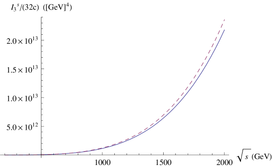
Figure 1: ${1\over 32c}I_{3}^{s}$ as a function of $\sqrt{s}$ for the $p\bar{p}$ collision. The dashed and continuous curves respectively represent two sets of parameters: $m_{H}=10$ GeV, $m_{f}=4.5$ GeV and $m_{H}=30$ GeV, $m_{f}=35$ GeV.

In Fig. 1, we display ${1\over 32c}I_{3}^{s}$ versus the c.m. energy $\sqrt{s}$ of the $p\bar{p}$ by the numerical method. Notice that the displayed ${1\over 32c}I_{3}^{s}$ is not the real cross section since the dynamical factor $c$ given in the original reference has not been included and the real cross section is $I_{3}^{s}$ (so the decay behavior of $I_{3}$ at high energy can not be observed from this Figure). Here, we emphasize two points. First, by our spinor method, almost all calculations have been reduced to reading out the residues of poles and making some algebraic manipulations. Thus although the analytic expression looks long, the calculation is kindly trivial.

Second, we can take appropriate integration order to simplify the process according to the structure of the integrand. Usually we should first perform the integrations over those variables, with respect to which the structure of the integrand is relatively simple. In this example, we have leave $k$ as the last integration variable. This is because the integrand Eq. (68) does not contain $h$ explicitly.

Notice that different integration ordering, i.e., integrating over $p_{1}$ first and then $p_{2}$ or integrating over $p_{2}$ first and then $p_{1}$, will in general give different-looking expressions. For example, in the expression of (47), we have fixed arbitrarily the ordering $m_{1},m_{2},m_{3},m_{4}$. Different ordering will end up with different integration regions although the final result should be the same. Furthermore, if we have left one particle un-integrated while others have been integrated, then we will get the corresponding differential cross section for this particle. Thus different integration ordering will give different differential cross sections for different particles.

5 Conclusion

Originating from the application of the spinor method to the massless case, in this paper, we have established the framework to process the massive case. From the examples presented in the paper, the advantages of our method is further manifested.

First, the manifestly Lorentz invariant form of the result in each step is gotten naturally. This ensures that the recursive method can be applied conveniently especially when the number of outgoing particles is large. In this process, we don’t need take any specified reference frame as when using the momentum integration method.

Second, the integration regions can be written straightforward according to Eq.(18), while with the momentum integration method, one has to pursue exhaustively to specify those of many variables (for example, angles and module variables). Note that in our method, though for the massive case the region is not so simple as the massless case, it is only the functions of mass and energy.

Finally, the salient point is that the constrained three-dimensional momentum space integration is reduced to an one-dimensional integration, plus possible Feynman integrations. However, in this so large simplification, we just pay a little extra price, namely the integration over $\lambda$ and $\widetilde{\lambda}$ which can be obtained by reading out residues of corresponding poles.

In this paper, our new method have shown out the value of practical calculations. As we have mentioned in the introduction, our method provides compact analytic expressions for cross section. Thus we can investigate the analytic structure using these expressions. We think it is an interesting direction. Also, in this paper we have just touched the tree-level result. It is our goal to combine these analytic expressions with one-loop result to see if we can improve current numerical NLO algorithm, especially the IR singularity substraction. A regularization scheme is mandatory and we need consider the general D-dimensional case. All these questions will be our future projects.

Acknowledgement:

We would like to thanks Dr. Kai Wang for providing us the references for our two real examples and Prof. Luo for stimulating discussions. The work is funded by Qiu-Shi funding as well as group funding 1A3000-172210115 from Zhejiang University, and Chinese NSF funding under contract No.10875104.

References

• [1] M. G. Albrow et al. [TeV4LHC QCD Working Group], arXiv:hep-ph/0610012.
• [2] Z. Bern et al. [NLO Multileg Working Group], [arXiv:hep-ph/0803.0494].
• [3] G. H. Brooijmans et al., arXiv:0802.3715 [hep-ph].
• [4] David E. Morrissey, Tilman Plehn, Tim M.P. Tait [arXiv:hep-ph/0912.3259]
• [5] S. Catani, M.H. Seymour, Nucl. Phys. B 485, 291 (1997) [Erratum-ibid. B 510 503 (1998)] [arXiv:hep-ph/9605323]
• [6] A. Gehrmann-De Ridder, T. Gehrmann and G. Heinrich, Nucl. Phys.  B 682, 265 (2004) [arXiv:hep-ph/0311276].
• [7] F. Maltoni, T. Stelzer, JHEP 0302, 027 (2003) [arXiv:hep-ph/0208156]; T. Sjostrand, S. Mrenna, P. Skands, JHEP 0605, 026 (2006) [axXiv:hep-ph/0603175]; M.L. Mangano, M. Moretti, F. Piccinini, R. Pittau, A.D. Polosa JHEP 0307, 001 (2003) [arXiv:hep-ph/0206293]; T. Gleisberg et al. JHEP 0902, 007 (2009) [arXiv:0811.4622]; S. Hoeche, F. Krauss, S. Schumann, F. Siegert, JHEP 0905, 053 (2009) [arXiv:0903.1219 [hep-ph]].
• [8] Z. Bern, L. J. Dixon, D. C. Dunbar and D. A. Kosower, Nucl. Phys. B 425, 217 (1994) [arXiv:hep-ph/9403226].
• [9] Z. Bern, L. J. Dixon, D. C. Dunbar and D. A. Kosower, Nucl. Phys.  B 435, 59 (1995) [arXiv:hep-ph/9409265].
• [10] E. Witten, Commun. Math. Phys.  252, 189 (2004)
• [11] F. Cachazo, P. Svrcek and E. Witten, JHEP 0410, 077 (2004)
• [12] R. Britto, F. Cachazo and B. Feng, Phys. Rev. D 71, 025012 (2005)
• [13] R. Britto, E. Buchbinder, F. Cachazo and B. Feng, Phys. Rev. D 72, 065012 (2005) [arXiv:hep-ph/0503132].
• [14] R. Britto, B. Feng and P. Mastrolia, Phys. Rev. D 73, 105004 (2006)
• [15] B. Feng, R. Huang, Y. Jia, M. Luo, H. Wang, Phys. Rev. D 81, 016003 (2010) [arXiv:hep-ph/0905.2715].
• [16] C. Anastasiou, R. Britto, B. Feng, Z. Kunszt and P. Mastrolia, Phys. Lett.  B 645, 213 (2007) [arXiv:hep-ph/0609191].
• [17] C. Anastasiou, R. Britto, B. Feng, Z. Kunszt and P. Mastrolia, JHEP 0703, 111 (2007) [arXiv:hep-ph/0612277].
• [18] B. Feng, G. Yang Nucl. Phys. B 811 305 (2009) [arXiv:hep-ph/0806.4016 ]
• [19] P. Kalyniak, John N. Ng, and P. Zakarauskas, Phys. Rev. D 29, 502(1984)
• [20] John N. Ng, and Pierre Zakarauskas, Phys. Rev. D 29, 876(1984)