Light-front quark model analysis of the exclusive rare $B_{c}\to D_{(s)}(\ell^{+}\ell^{-},\nu_{\ell}\bar{\nu}_{\ell})$ decays

Abstract

We investigate the exclusive rare $B_{c}\to D_{(s)}\nu_{\ell}\bar{\nu_{\ell}}$ and $B\to D_{(s)}\ell^{+}\ell^{-}$ ($\ell=e,\mu,\tau$) decays within the standard model and the light-front quark model constrained by the variational principle for the QCD motivated effective Hamiltonian. The form factors $f_{\pm}(q^{2})$ and $f_{T}(q^{2})$ are obtained from the analytic continuation method in the $q^{+}=0$ frame. While the form factors $f_{+}(q^{2})$ and $f_{T}(q^{2})$ are free from the zero-mode, the form factor $f_{-}(q^{2})$ is not free from the zero-mode in the $q^{+}=0$ frame. We discuss the covariance(i.e. frame-independence) of our model calculation and quantify the zero-mode contributions to $f_{-}(q^{2})$ for $B_{c}\to D_{(s)}$ decays. The branching ratios and the longitudinal lepton polarization asymmetries are calculated with and without the long-distance contributions. Our numerical results for the non-resonant branching ratios for $B_{c}\to D(D_{s})\sum\nu_{\ell}\bar{\nu_{\ell}}$ and $B_{c}\to D(D_{s})\ell^{+}\ell^{-}$ are in the order of $10^{-8}\;(10^{-7})$ and $10^{-9}\;(10^{-8})$, respectively. The averaged values of the lepton polarization asymmetries obtained from the linear (harmonic oscillator) potential parameters are found to be $-0.99\;(-0.99)$ for $B_{c}\to D\mu^{+}\mu^{-}$ and $-0.16\;(-0.15)$ for $B_{c}\to D\tau^{+}\tau^{-}$, and $-0.98\;(-0.98)$ for $B_{c}\to D_{s}\mu^{+}\mu^{-}$ and $-0.14\;(-0.12)$ for $B_{c}\to D_{s}\tau^{+}\tau^{-}$, respectively.

I Introduction

The LHCb (Large Hadron Collider beauty) experiment dedicated to heavy flavor physics at LHC make precision tests of the standard model (SM) and beyond the SM ever more promising. Its primary goal is to look for indirect evidence of new physics in CP violation and rare decays of beauty and charm hadrons. Especially, a stringent test on the unitarity of Cabibbo-Kobayashi-Maskawa (CKM) mixing matrix in the SM will be made by this facility. With the upcoming chances that a numerous number of $B_{c}$ mesons will be produced at LHC, one might explore the exclusive rare $B_{c}$ decays to $(D,D_{s})\ell^{+}\ell^{-}$ and $(D,D_{s})\nu_{\ell}\bar{\nu}_{\ell}$ ($\ell=e,\mu,\tau$) induced by the flavor-changing neutral current $b\to(d,s)$ transitions. Since in the SM the rare $B_{c}$ decays are forbidden at tree level and occur at the lowest order only through one-loop diagrams GWS ; BM ; Misiak ; TI ; AMM ; KMS ; AKS , they are well suited to test the SM and search for physics beyond the SM. In such exclusive rare decays, any reliable extraction of the perturbative effects encoded in the Wilson coefficients of the effective Hamiltonian requires an accurate separation of the nonperturbative contributions, which are encoded in the hadronic form factors. This part of the calculation is model dependent since it involves nonperturbative QCD. Therefore, a reliable estimate of the hadronic form factors for the exclusive rare $B_{c}$ decays is very important to make correct predictions within and beyond the SM.

There are some theoretical approaches to the calculations of the exclusive rare $B_{c}\to(D,D_{s})\ell^{+}\ell^{-}$ and $B_{c}\to(D,D_{s})\nu_{\ell}\bar{\nu}_{\ell}$ decay modes. Although we may not be able to list them all, we may note here the following works: the relativistic constituent quark model Faessler , the light-front(LF) and constituent quark model (CQM) Geng , and three point QCD sum rules Azizi . The rare $B_{c}\to D_{s}\ell^{+}\ell^{-}$ decay beyond the SM has also been studied in Yilmaz . Perhaps, one of the most well-suited formulations for the analysis of exclusive processes involving hadrons may be provided in the framework of light-front quantization BPP .

The purpose of this paper is to extend our our light-front quark model (LFQM) CJ1 ; CJ_PLB1 ; JC_E ; CJK ; ChoiRD ; CJBc ; CJNRD based on the QCD-motivated effective LF Hamiltonian to calculate the hadronic form factors, decay rates and the longitudinal lepton polarization asymmetries (LPAs) for the exclusive rare $B_{c}\to(D,D_{s})\ell^{+}\ell^{-}$ and $B_{c}\to(D,D_{s})\nu_{\ell}\bar{\nu}_{\ell}$ decays within the SM. The LPA, as another parity-violating observable, is an important asymmetry Hew and could be measured by the LHCb experiment. In particular, the $\tau$ channel would be more accessible experimentally than $e$- or $\mu$-channels since the LPAs in the SM are known to be proportional to the lepton mass.

In our previous LFQM analysis CJBc ; CJNRD , we have analyzed the exclusive semileptonic $B_{c}\to(D,\eta_{c},B,B_{s})\ell\nu_{\ell}$ decays CJBc and the nonleptonic two-body decays of $B_{c}$ mesons such as $B_{c}\to(D_{(s)},\eta_{c},B_{(s)})(P,V)$ decays CJNRD (here $P$ and $V$ denote pseudoscalar and vector mesons, respectively). Our LFQM CJ1 ; CJ_PLB1 ; JC_E ; CJK ; ChoiRD ; CJBc ; CJNRD analysis compared to the other LFQM has several salient features: (i) We have implemented the variational principle to the QCD motivated effective LF Hamiltonian to enable us to analyze the meson mass spectra and to find optimized model parameters CJ1 ; CJ_PLB1 . (ii) The weak form factors $f_{\pm}(q^{2})$ for the semileptonic decays between two pseudoscalar mesons are obtained in the Drell-Yan-West ($q^{+}=q^{0}+q^{3}=0$) frame DYW (i.e., $q^{2}=-{\bf q}^{2}_{\perp}<0$) and then analytically continued to the timelike region by changing ${\bf q}^{2}_{\perp}$ to $-q^{2}$ in the form factor. The covariance (i.e., frame independence) of our model has been checked CJBc by performing the LF calculation in the $q^{+}=0$ frame in parallel with the manifestly covariant calculation using the exactly solvable covariant fermion field theory model in $(3+1)$ dimensions. We also found the zero-mode Zero contribution to the form factor $f_{-}(q^{2})$ and identified CJBc the zero-mode operator that is convoluted with the initial and final state LF wave functions.

Specifically, in the present analysis of exclusive rare $B_{c}\to(D,D_{s})\ell^{+}\ell^{-}$ and $B_{c}\to(D,D_{s})\nu_{\ell}\bar{\nu}_{\ell}$ decays, three independent hadronic form factors, i.e. $f_{+}(q^{2})$, $f_{-}(q^{2})$ from the vector-axial vector current, and $f_{T}(q^{2})$ from the tensor current, are needed. While the two form factors $f_{+}$ and $f_{T}$ can be obtained only from the valence contributions in the $q^{+}=0$ frame without encountering the zero-mode complication, the form factor $f_{-}(q^{2})$ receives the higher Fock state contribution (i.e., the zero mode in the $q^{+}=0$ frame or the nonvalence contribution in the $q^{+}>0$ frame) within the framework of LF quantization. Thus, it is necessary to include either the zero-mode contribution (if working in the $q^{+}=0$ frame) or the nonvalence contribution (if working in the $q^{+}>0$ frame) to obtain the form factor $f_{-}(q^{2})$. In this work, we shall use the form factors $f_{+}(q^{2})$ and $f_{-}(q^{2})$ for the exclusive semileptonic $B_{c}\to(D,D_{s})$ decays obtained in CJBc and the form factor $f_{T}(q^{2})$ obtained in CJK for the analysis of $B\to K\ell^{+}\ell^{-}$ decay. Especially, the Lorentz covariance of our tensor form factor $f_{T}(q^{2})$ is discussed in this work. The present investigation further constrains the phenomenological parameters and extends the applicability of our LFQM CJ1 ; CJ_PLB1 to the wider range of hadronic phenomena.

The paper is organized as follows. In Sec. II, the SM operator basis, describing the $b\to(d,s)\ell^{+}\ell^{-}$ and $b\to(d,s)\nu_{\ell}\bar{\nu}_{\ell}$ transitions, is briefly presented. In Sec. III, we briefly describe the formulation of our LFQM and the procedure of fixing the model parameters using the variational principle for the QCD motivated effective Hamiltonian. We present the LF covariant forms of the form factors $f_{\pm}(q^{2})$ and $f_{T}(q^{2})$ obtained in the $q^{+}=0$ frame. In Sec. IV, our numerical results, i.e. the form factors, decay rates, and the LPAs for the rare $B_{c}\to(D,D_{s})\ell^{+}\ell^{-}$ and $B_{c}\to(D,D_{s})\nu_{\ell}\bar{\nu}_{\ell}$ decays are presented. Summary and discussion of our main results follow in Sec. V. In the Appendix, we explicitly show the covariance of $f_{T}(q^{2})$ by performing the LF calculation in parallel with the manifestly covariant one using the exactly solvable covariant fermion field theory model in $(3+1)$ dimensions.

II Effective Hamiltonian

In the SM, the exclusive rare $B_{c}\to D_{q}(\ell^{+}\ell^{-},\nu_{\ell}\bar{\nu}_{\ell})$ decays are at the quark level described by the loop $b\to q(\ell^{+}\ell^{-},\nu_{\ell}\bar{\nu}_{\ell})(q=d,s)$ transitions, and receive contributions from the $Z(\gamma)$-penguin and $W$-box diagrams as shown in Fig. 1.

Figure 1: Loop diagrams for $B_{c}\to D_{q}(\ell^{+}\ell^{-},\nu_{\ell}\bar{\nu}_{\ell})(q=d,s)$ transitions.

The effective Hamiltonian responsible for the $b\to q\ell^{+}\ell^{-}(q=d,s)$ decay processes can be represented in terms of the Wilson coefficients, $C_{7}^{\rm eff},C_{9}^{\rm eff}$ and $C_{10}$ as BM

$${\cal H}^{\ell^{+}\ell^{-}}_{\rm eff} = \frac{G_{F}\alpha_{\rm em}}{2\sqrt{2}\pi}V_{tb}V^{*}_{tq}\biggl{[}C^{\rm eff}_{9}\bar{q}\gamma_{\mu}(1-\gamma_{5})b\bar{\ell}\gamma^{\mu}\ell$$ (1)

$$+C_{10}\bar{q}\gamma_{\mu}(1-\gamma_{5})b\bar{\ell}\gamma^{\mu}\gamma_{5}\ell$$

$$-C_{7}^{\rm eff}\frac{2m_{b}}{q^{2}}\bar{q}i\sigma_{\mu\nu}q^{\nu}(1+\gamma_{5})b\bar{\ell}\gamma^{\mu}\ell\biggr{]},$$

where $G_{F}$ is the Fermi constant, $\alpha_{\rm em}$ is the fine structure constant, and $V_{ij}$ are the CKM matrix elements. The relevant Wilson coefficients $C_{i}$ can be found in Ref. BM . The effective Hamiltonian responsible for the $b\to q\nu_{\ell}\bar{\nu}_{\ell}(q=d,s)$ decay processes is given by MN

$${\cal H}^{\nu_{\ell}\bar{\nu}_{\ell}}_{\rm eff} = \frac{G_{F}\alpha_{\rm em}}{2\sqrt{2}\pi}V_{tb}V^{*}_{tq}\frac{X(x_{t})}{\sin^{2}\theta_{W}}\bar{q}\gamma_{\mu}(1-\gamma_{5})b$$ (2)

$$\times \bar{\nu}_{\ell}\gamma^{\mu}(1-\gamma_{5})\nu_{\ell},$$

where $x_{t}=(m_{t}/M_{W})^{2}$ and $X(x_{t})$ is an Inami-Lim function TI , which is given by

$$X(x)=\frac{x}{8}\biggl{(}\frac{2+x}{x-1}+\frac{3x-6}{(x-1)^{2}}\ln x\biggr{)}.$$ (3)

The long distance (LD) contribution to the exclusive $B_{c}\to D_{q}(q=d,s)$ decays is contained in the meson matrix elements of the bilinear quark currents appearing in ${\cal H}^{\ell^{+}\ell^{-}}_{\rm eff}$ and ${\cal H}^{\nu_{\ell}\bar{\nu_{\ell}}}_{\rm eff}$. In the matrix elements of the hadronic currents for $B_{c}\to D_{q}$ transitions, the parts containing $\gamma_{5}$ do not contribute. Considering Lorentz and parity invariances, these matrix elements can be parametrized in terms of hadronic form factors as follows:

$$J^{\mu}\equiv\langle D_{q}|\bar{q}\gamma^{\mu}b|B_{c}\rangle=f_{+}(q^{2})P^{\mu}+f_{-}(q^{2})q^{\mu},$$ (4)

and

$$J^{\mu}_{T} \equiv \langle D_{q}|\bar{q}i\sigma^{\mu\nu}q_{\nu}b|B_{c}\rangle$$ (5)

$$= \frac{f_{T}(q^{2})}{M_{B_{c}}+M_{D_{q}}}[q^{2}P^{\mu}-(M^{2}_{B_{c}}-M^{2}_{D_{q}})q^{\mu}],$$

where $P=P_{B_{c}}+P_{D_{q}}$ and $q=P_{B_{c}}-P_{D_{q}}$ is the four-momentum transfer to the lepton pair and $4m^{2}_{\ell}\leq q^{2}\leq(M_{B_{c}}-M_{D_{q}})^{2}$. We use the convention $\sigma^{\mu\nu}=(i/2)[\gamma^{\mu},\gamma^{\nu}]$ for the antisymmetric tensor. Sometimes it is useful to express Eq. (4) in terms of $f_{+}(q^{2})$ and $f_{0}(q^{2})$, which are related to the exchange of $1^{-}$ and $0^{+}$, respectively, and satisfy the following relations:

$$f_{+}(0)=f_{0}(0),\;f_{0}(q^{2})=f_{+}(q^{2})+\frac{q^{2}}{M^{2}_{B_{c}}-M^{2}_{D_{q}}}f_{-}(q^{2}).$$ (6)

With the help of the effective Hamiltonian in Eq. (1) and Eqs. (4) and (5), the transition amplitude ${\cal M}=\langle D_{q}\ell^{+}\ell^{-}|{\cal H}_{\rm eff}|B_{c}\rangle$ for the $B_{c}\to D_{q}\ell^{+}\ell^{-}$ decay can be written as

$${\cal M} = \frac{G_{F}\alpha_{\rm em}}{2\sqrt{2}\pi}V_{tb}V^{*}_{tq}\biggl{\{}\biggl{[}C^{\rm eff}_{9}J_{\mu}-\frac{2m_{b}}{q^{2}}C^{\rm eff}_{7}J^{T}_{\mu}\biggr{]}\bar{\ell}\gamma^{\mu}\ell$$ (7)

$$\hskip 71.13188pt+C_{10}J_{\mu}\bar{\ell}\gamma^{\mu}\gamma_{5}\ell\biggr{\}}.$$

The differential decay rate for the exclusive rare $B_{c}\to D_{q}\ell^{+}\ell^{-}$ with nonzero lepton mass is given by GK ; MN

$$\frac{d\Gamma}{ds} = \frac{M^{5}_{B_{c}}G^{2}_{F}}{3\cdot 2^{9}\pi^{5}}\alpha^{2}_{\rm em}|V_{tb}V^{*}_{tq}|^{2}\phi_{H}^{1/2}\biggl{(}1-\frac{4t}{s}\biggr{)}^{1/2}$$ (8)

$$\times\biggl{[}\phi_{H}\biggl{(}1+\frac{2t}{s}\biggr{)}{\cal F}_{1}+12t{\cal F}_{2}\biggr{]},$$

where

$${\cal F}_{1} = \biggl{|}C^{\rm eff}_{9}f_{+}-\frac{2\hat{m_{b}}C^{\rm eff}_{7}}{1+\sqrt{r}}f_{T}\biggr{|}^{2}+|C_{10}f_{+}|^{2},$$

$${\cal F}_{2} = |C_{10}|^{2}\biggl{[}(1+r-\frac{s}{2})|f_{+}|^{2}+(1-r)f_{+}f_{-}+\frac{s}{2}|f_{-}|^{2}\biggr{]},$$

$$\phi_{H} = (s-1-r)^{2}-4r,$$

with $s=q^{2}/M^{2}_{B_{c}}$, $t=m^{2}_{\ell}/M^{2}_{B_{c}}$, $\hat{m_{b}}=m_{b}/M_{B_{c}}$ and $r=M^{2}_{D_{q}}/M^{2}_{B_{c}}$. The differential decay rate in Eq. (8) may be written in terms of ($f_{+},f_{0},f_{T}$) instead of ($f_{+},f_{-},f_{T}$) as discussed in CJK . Note also from Eqs. (8) and (II) that the form factor $f_{-}(q^{2})$ contributes only in the nonzero lepton ($m_{\ell}\neq 0$) mass limit. Dividing Eq. (8) by the total width of the $B_{c}$ meson, one can obtain the differential branching ratio $d{\rm BR}(B_{c}\to D_{q}\ell^{+}\ell^{-})/ds=(d\Gamma(B_{c}\to D_{q}\ell^{+}\ell^{-})/\Gamma_{\rm tot})/ds$.

The differential decay rate for $B_{c}\to D_{q}\nu_{\ell}\bar{\nu}_{\ell}$ can be easily obtained from the corresponding formula Eq. (8) for $B_{c}\to D_{q}\ell^{+}\ell^{-}$ by the replacement

$$\hat{m}_{\ell}\to 0,\;C_{7}^{\rm eff}\to 0,\;C^{\rm eff}_{9}\to\frac{X(x_{t})}{\sin^{2}\theta_{W}},\;C_{10}\to-\frac{X(x_{t})}{\sin^{2}\theta_{W}},$$ (10)

where $\theta_{W}$ is the Weinberg angle. As another interesting observable, the LPA, is defined as

$$P_{L}(s)=\frac{d\Gamma_{h=-1}/ds-d\Gamma_{h=1}/ds}{d\Gamma_{h=-1}/ds+d\Gamma_{h=1}/ds},$$ (11)

where $h=+1\;(-1)$ denotes right (left) handed $\ell^{-}$ in the final state. From Eq. (8), one obtains for $B_{c}\to D_{q}\ell^{+}\ell^{-}$

$$P_{L}(s)=\frac{2\biggl{(}1-4\frac{t}{s}\biggr{)}^{1/2}\phi_{H}C_{10}f_{+}\biggl{[}f_{+}{\rm Re}C^{\rm eff}_{9}-\frac{2\hat{m_{b}}C^{\rm eff}_{7}}{1+\sqrt{r}}f_{T}\biggr{]}}{\biggl{[}\phi_{H}\biggl{(}1+2\frac{t}{s}\biggr{)}{\cal F}_{1}+12t{\cal F}_{2}\biggr{]}}.$$ (12)

Because of the experimental difficulties of studying the polarizations of each lepton depending on $s$ and the Wilson coefficients, it would be better to eliminate the dependence of the LPA on $s$, by considering the averaged form over the entire kinematical region. The averaged LPA is defined by

$$\langle P_{L}\rangle=\frac{\int^{(1-\sqrt{r})^{2}}_{4t}P_{L}\frac{dBR}{ds}ds}{\int^{(1-\sqrt{r})^{2}}_{4t}\frac{dBR}{ds}ds}.$$ (13)

III Form factors in Light-front quark model

The key idea in our LFQM CJ1 ; CJ_PLB1 for mesons is to treat the radial wave function as a trial function for the variational principle to the QCD-motivated effective Hamiltonian saturating the Fock state expansion by the constituent quark and antiquark. The QCD-motivated Hamiltonian for a description of the ground state meson mass spectra is given by

$$H_{q\bar{q}}|\Psi^{JJ_{z}}_{nlm}\rangle = \biggl{[}\sqrt{m^{2}_{q}+{\vec{k}}^{2}}+\sqrt{m^{2}_{\bar{q}}+{\vec{k}}^{2}}+V_{q\bar{q}}\biggr{]}|\Psi^{JJ_{z}}_{nlm}\rangle,$$ (14)

$$= [H_{0}+V_{q\bar{q}}]|\Psi^{JJ_{z}}_{nlm}\rangle=M_{q\bar{q}}|\Psi^{JJ_{z}}_{nlm}\rangle,$$

where ${\vec{k}}=({\bf k}_{\perp},k_{z})$ is the three-momentum of the constituent quark, $M_{q\bar{q}}$ is the mass of the meson, and $|\Psi^{JJ_{z}}_{nlm}\rangle$ is the meson wave function. We use two interaction potentials $V_{q\bar{q}}$; (i) Coulomb plus harmonic oscillator (HO) and (ii) Coulomb plus linear confining potentials. The hyperfine interaction essential to distinguish pseudoscalar and vector mesons is also included; viz.,

$$V_{q\bar{q}}=V_{0}+V_{\rm hyp}=a+{\cal V}_{\rm conf}-\frac{4\alpha_{s}}{3r}+\frac{2}{3}\frac{{\bf S}_{q}\cdot{\bf S}_{\bar{q}}}{m_{q}m_{\bar{q}}}\nabla^{2}V_{\rm coul},$$ (15)

where ${\cal V}_{\rm conf}=br\;(r^{2})$ for the linear (HO) potential and $\langle{\bf S}_{q}\cdot{\bf S}_{\bar{q}}\rangle=1/4\;(-3/4)$ for the vector (pseudoscalar) meson. Using this Hamiltonian, we analyze the meson mass spectra and various wave-function-related observables, such as decay constants, electromagnetic form factors of mesons in a spacelike region, and the weak form factors for the exclusive semileptonic and rare decays of pseudoscalar mesons in the timelike region CJ1 ; CJ_PLB1 ; JC_E ; CJK ; ChoiRD ; CJBc .

The momentum-space LF wave function of the ground state pseudoscalar mesons is given by

$$\Psi^{00}_{100}(x_{i},{\bf k}_{i\perp},\lambda_{i})={\cal R}^{00}_{\lambda_{1}\lambda_{2}}(x_{i},{\bf k}_{i\perp})\phi(x_{i},{\bf k}_{i\perp}),$$ (16)

where $\phi(x_{i},{\bf k}_{i\perp})$ is the radial wave function and ${\cal R}^{00}_{\lambda_{1}\lambda_{2}}$ is the spin-orbit wave function. The model wave function in Eq. (16) is represented by the Lorentz-invariant internal variables, $x_{i}=p^{+}_{i}/P^{+}$, ${\bf k}_{i\perp}={\bf p}_{i\perp}-x_{i}{\bf P}_{\perp}$ and $\lambda_{i}$, where $P^{\mu}=(P^{+},P^{-},{\bf P}_{\perp})=(P^{0}+P^{3},(M^{2}+{\bf P}^{2}_{\perp})/P^{+},{\bf P}_{\perp})$ is the momentum of the meson $M$, and $p^{\mu}_{i}$ and $\lambda_{i}$ are the momenta and the helicities of constituent quarks, respectively. The covariant forms of the spin-orbit wave function for pseudoscalar mesons is given by

$${\cal R}_{\lambda_{1}\lambda_{2}}^{00} = \frac{-\bar{u}_{\lambda_{1}}(p_{1})\gamma_{5}v_{\lambda_{2}}(p_{2})}{\sqrt{2}\tilde{M_{0}}},$$ (17)

where $\tilde{M_{0}}=\sqrt{M^{2}_{0}-(m_{1}-m_{2})^{2}}$ and $M^{2}_{0}=\sum_{i=1}^{2}({\bf k}^{2}_{i\perp}+m^{2}_{i})/x_{i}$ is the boost invariant meson mass square obtained from the free energies of the constituents in mesons. For the radial wave function $\phi$, we use the Gaussian wave function:

$$\phi(x_{i},{\bf k}_{i\perp})=\frac{4\pi^{3/4}}{\beta^{3/2}}\sqrt{\frac{\partial k_{z}}{\partial x}}{\rm exp}(-{\vec{k}}^{2}/2\beta^{2}),$$ (18)

where $\beta$ is the variational parameter and $\sqrt{\partial k_{z}/\partial x}$ is the Jacobian of the variable transformation $\{x,{\bf k}_{\perp}\}\to{\vec{k}}=({\bf k}_{\perp},k_{z})$.

We apply our variational principle to the QCD-motivated effective Hamiltonian first to evaluate the expectation value of the central Hamiltonian $H_{0}+V_{0}$, i.e., $\langle\phi|(H_{0}+V_{0})|\phi\rangle$ with a trial function $\phi(x_{i},{\bf k}_{i\perp})$ that depends on the variational parameter $\beta$. Once the model parameters are fixed by minimizing the expectation value $\langle\phi|(H_{0}+V_{0})|\phi\rangle$, then the mass eigenvalue of each meson is obtained as $M_{q\bar{q}}=\langle\phi|(H_{0}+V_{q\bar{q}})|\phi\rangle$. A more detailed procedure for determining the model parameters of light- and heavy-quark sectors can be found in our previous works CJ1 ; CJ_PLB1 ; CJBc .

The form factors $f_{\pm}(q^{2})$ and $f_{T}(q^{2})$ for $B_{c}(q_{1}\bar{q})\to P(q_{2}\bar{q})$ decays are obtained from the $q^{+}=0$ frame. Although the form factors $f_{\pm}(q^{2})$ and $f_{T}(q^{2})$ are given in CJBc and CJK , respectively, we list them here again:

$$f_{+}(q^{2}) = \int^{1}_{0}dx\int\frac{d^{2}{\bf k}_{\perp}}{16\pi^{3}}\frac{\phi_{1}(x,{\bf k}_{\perp})}{\sqrt{{\cal A}_{1}^{2}+{\bf k}^{2}_{\perp}}}\frac{\phi_{2}(x,{\bf k}^{\prime}_{\perp})}{\sqrt{{\cal A}_{2}^{2}+{\bf k}^{\prime 2}_{\perp}}}({\cal A}_{1}{\cal A}_{2}+{\bf k}_{\perp}\cdot{\bf k^{\prime}}_{\perp}),$$

$$f_{-}(q^{2}) = \int^{1}_{0}(1-x)dx\int\frac{d^{2}{\bf k}_{\perp}}{16\pi^{3}}\frac{\phi_{1}(x,{\bf k}_{\perp})}{\sqrt{{\cal A}^{2}_{1}+{\bf k}^{2}_{\perp}}}\frac{\phi_{2}(x,{\bf k^{\prime}}_{\perp})}{\sqrt{{\cal A}^{2}_{2}+{\bf k}^{\prime 2}_{\perp}}}\biggl{\{}-x(1-x)M^{2}_{1}-{\bf k}^{2}_{\perp}-m_{1}m+(m_{2}-m){\cal A}_{1}$$

$$+2\frac{q\cdot P}{q^{2}}\biggl{[}{\bf k}^{2}_{\perp}+2\frac{({\bf k}_{\perp}\cdot{\bf q}_{\perp})^{2}}{q^{2}}\biggr{]}+2\frac{({\bf k}_{\perp}\cdot{\bf q}_{\perp})^{2}}{q^{2}}+\frac{{\bf k}_{\perp}\cdot{\bf q}_{\perp}}{q^{2}}[M^{2}_{2}-(1-x)(q^{2}+q\cdot P)+2xM^{2}_{0}$$

$$-(1-2x)M^{2}_{1}-2(m_{1}-m)(m_{1}+m_{2})]\biggr{\}},$$

$$f_{T}(q^{2}) = (M_{1}+M_{2})\int^{1}_{0}(1-x)dx\int\frac{d^{2}{\bf k}_{\perp}}{16\pi^{3}}\frac{\phi_{1}(x,{\bf k}_{\perp})}{\sqrt{{\cal A}^{2}_{1}+{\bf k}^{2}_{\perp}}}\frac{\phi_{2}(x,{\bf k^{\prime}}_{\perp})}{\sqrt{{\cal A}^{2}_{2}+{\bf k}^{\prime 2}_{\perp}}}\biggl{[}(m_{1}-m_{2})\frac{{\bf k}_{\perp}\cdot{\bf q}_{\perp}}{{\bf q}^{2}_{\perp}}+{\cal A}_{1}\biggr{]},$$ (19)

where ${\bf k^{\prime}}_{\perp}={\bf k}_{\perp}+(1-x){\bf q}_{\perp}$, ${\cal A}_{i}=(1-x)m_{i}+xm$ ($i=1,2$), and $q\cdot P=M^{2}_{1}-M^{2}_{2}$ with $M_{1}$ and $M_{2}$ being the physical masses of the initial and final state mesons, respectively. The explicit covariances of $f_{\pm}(q^{2})$ and $f_{T}(q^{2})$ are proven in CJBc and in the appendix of this work, respectively. Since the form factors $f_{\pm}(q^{2})$ and $f_{T}(q^{2})$ in Eq. (III) are defined in the spacelike ($q^{2}=-{\bf q}^{2}_{\perp}<0$) region, we then analytically continue them to the timelike $q^{2}>0$ region by changing ${\bf q}^{2}_{\perp}$ to $-q^{2}$ in the form factors. We should note that our analytic method is reliable in the entire physical region of the exclusive rare decay since the first unitary branch point occurs just right after the zero-recoil point, $q^{2}=(M_{1}-M_{2})^{2}$.

We also compare our analytic solutions with the double pole parametric form given by

$$f_{i}(q^{2})=\frac{f_{i}(0)}{1-\sigma_{1}s+\sigma_{2}s^{2}},$$ (20)

where $\sigma_{1}$ and $\sigma_{2}$ are the fitted parameters.

IV Numerical results

In our numerical calculations for the exclusive rare $B_{c}\to(D,D_{s})(\nu_{\ell}\bar{\nu_{\ell}})$ and $B_{c}\to(D,D_{s})(\ell^{+}\ell^{-})$ decays, we use two sets of model parameters ($m_{q},\beta$) for the linear and HO confining potentials given in Table 1 CJ1 ; CJ_PLB1 ; CJBc . Although our predictions CJBc of ground state heavy meson masses are overall in good agreement with the experimental values, we use the experimental meson masses Data08 in the computations of the decay widths to reduce possible theoretical uncertainties.

Table 1: Model parameters ($m_{q},\beta$) [GeV] for $D,D_{s}$ and $B_{c}$ mesons used in our analysis. $q=u$ and $d$.

Model	$m_{q}$	$m_{s}$	$m_{c}$	$m_{b}$	$\beta_{qc}$	$\beta_{sc}$	$\beta_{cb}$
Linear	0.22	0.45	1.8	5.2	0.4679	0.5016	0.8068
HO	0.25	0.48	1.8	5.2	0.4216	0.4686	1.0350

Note that in the numerical calculations we take $(m_{c},m_{b})=(1.8,5.2)$ GeV in all formulas except in the Wilson coefficient $C^{\rm eff}_{9}$, where $(m_{c},m_{b,\rm pole})=(1.4,4.8)$ GeV have been commonly used BM . For the numerical values of the Wilson coefficients, we use the results given by Ref. BM :

$$C_{1} = -0.248,\;C_{2}=1.107,\;C_{3}=0.011,$$

$$C_{4} = -0.026,\;C_{5}=0.007,\;C_{6}=-0.031,$$

$$C^{\rm eff}_{7} = -0.313,\;C_{9}=4.344,\;C_{10}=-4.669,$$ (21)

and other input parameters are $|V_{tb}V^{*}_{ts}|=0.039$, $|V_{tb}V^{*}_{td}|=0.008$, $\alpha_{\rm em}^{-1}=129$, $M_{W}=80.43$ GeV, $m_{t}=171.3$ GeV, $\sin^{2}\theta_{W}=0.2233$, and $\tau_{B_{c}}=0.46$ ps. The effective Wilson coefficient $C^{\rm eff}_{9}$ taking into account both the short distance (SD) and the LD contributions from $c\bar{c}$ resonance states ($J/\psi,\psi^{\prime},\cdots$) has the following form BM

$$C^{\rm eff}_{9}(s)=C_{9}+Y_{SD}(s)+Y_{LD}(s),$$ (22)

where the explicit forms of $Y_{SD}(s)$ and $Y_{LD}(s)$ can be found in BM ; Faessler . For the LD contribution $Y_{LD}(s)$, we include two $c\bar{c}$ resonant states $J/\psi(1S)$ and $\psi^{\prime}(2S)$ and use $\Gamma(J/\psi\to\ell^{+}\ell^{-})=5.26\times 10^{-6}$ GeV, $M_{J/\psi}=3.1$ GeV, $\Gamma_{J/\psi}=87\times 10^{-6}$ GeV for $J/\psi(1S)$ and $\Gamma(\psi^{\prime}\to\ell^{+}\ell^{-})=2.12\times 10^{-6}$ GeV, $M_{\psi^{\prime}}=3.69$ GeV, $\Gamma_{\psi^{\prime}}=277\times 10^{-6}$ GeV for $\psi^{\prime}(2S)$ Data08 .

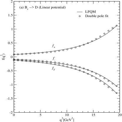
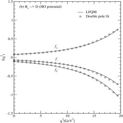
Figure 2: The weak form factors (solid line) for $B_{c}\to D$ transitions obtained from the (a) linear and (b) HO potential parameters. The circles stand for the results from the double pole fits.

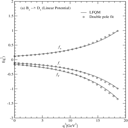
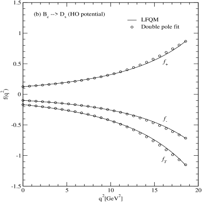
Figure 3: The weak form factors (solid line) for $B_{c}\to D_{s}$ transitions obtained from the (a) linear and (b) HO potential parameters. The circles stand for the results from the double pole fits.

In Figs. 2 and 3, we show the $q^{2}$ dependences of the form factors $f_{\pm}(q^{2})$ and $f_{T}(q^{2})$ (solid line) for the $B_{c}\to D$ and $B_{c}\to D_{s}$ transitions obtained from the (a) linear and (b) HO potential parameters, respectively. We also include the results (circles) obtained from the double pole form given by Eq. (20). As one can see from Figs. 2 and 3, our analytic solutions are well approximated by the double pole form.

The form factors at the zero-recoil point (i.e., $q^{2}=q^{2}_{\rm max})$ correspond to the overlap integral of the initial and final state meson wave functions. The maximum-recoil point (i.e., $q^{2}=0$) corresponds to a final state meson recoiling with the maximum three-momentum $|{\vec{P}}_{D_{(s)}}|=(M^{2}_{B_{c}}-M^{2}_{D_{(s)}})/2M_{B_{c}}$ in the rest frame of the $B_{c}$ meson. For $B_{c}\to D$ transition, while the form factors at $q^{2}=0$ obtained from the linear [HO] potential parameters are $f_{+}(0)=0.086\;[0.079]$, $f_{-}(0)=-0.089\;[-0.070]$, and $f_{T}(0)=-0.120\;[-0.108]$, the form factors at $q^{2}=q^{2}_{\rm max}$ are $f_{+}(q^{2}_{\rm max})=1.129\;[0.752]$, $f_{-}(q^{2}_{\rm max})=-1.060\;[-0.723]$, and $f_{T}(q^{2}_{\rm max})=-1.319\;[-1.034]$. As for the zero-mode contribution to the form factor $f_{-}(q^{2})$, i.e. $f^{\rm Z.M.}_{-}(q^{2})=f_{-}(q^{2})-f^{\rm val}_{-}(q^{2})$ CJBc , we obtain the valence contribution to $f_{-}(q^{2})$ as $f^{\rm val}_{-}(0)=-0.096\;[-0.081]$ and $f^{\rm val}_{-}(q^{2}_{\rm max})=-1.132\;[-0.823]$ from the linear [HO] potential parameters. This estimates about $7\%\sim 15\%$ zero-mode contribution to $f_{-}(q^{2})$ for the $B_{c}\to D$ transition. For $B_{c}\to D_{s}$ transition, while the form factors at $q^{2}=0$ obtained from the linear [HO] potential parameters are $f_{+}(0)=0.120\;[0.126]$, $f_{-}(0)=-0.113\;[-0.099]$, and $f_{T}(0)=-0.163\;[-0.168]$, the form factors at $q^{2}=q^{2}_{\rm max}$ are $f_{+}(q^{2}_{\rm max})=0.992\;[0.868]$, $f_{-}(q^{2}_{\rm max})=-0.988\;[-0.719]$, and $f_{T}(q^{2}_{\rm max})=-1.342\;[-1.157]$. We also obtain the valence contribution to $f_{-}(q^{2})$ as $f^{\rm val}_{-}(0)=-0.121\;[-0.105]$ and $f^{\rm val}_{-}(q^{2}_{\rm max})=-1.114\;[-0.815]$ from the linear [HO] potential parameters. This also estimates about $7\%\sim 15\%$ zero-mode contribution to $f_{-}(q^{2})$ for the $B_{c}\to D_{s}$ transition.

Table 2: Results for form factors at $q^{2}=0$ of $B_{c}\to D\ell^{+}\ell^{-}/\nu_{\ell}\bar{\nu_{\ell}}$ decay and parameters $\sigma_{i}$ defined in Eq. (20).

Model	$f_{+}(0)$	$\sigma_{1}$	$\sigma_{2}$	$f_{-}(0)$	$\sigma_{1}$	$\sigma_{2}$	$f_{T}(0)$	$\sigma_{1}$	$\sigma_{2}$
Linear	0.086	$-3.50$	3.30	$-0.089$	$-3.38$	3.09	$-0.120$	$-3.35$	3.06
HO	0.079	$-3.20$	2.81	$-0.070$	$-3.28$	2.94	$-0.108$	$-3.18$	2.77
RCQM Faessler	0.186	$-3.48$	1.62	$-0.190$	$-2.44$	1.54	$-0.275$	$-2.40$	1.49
CQM Geng	0.123	$-3.35$	3.03	$-0.130$	$-3.63$	3.55	$-0.186$	$-3.52$	3.38
SR Azizi	0.22	$-1.10$	$-2.48$	$-0.29$	$-0.63$	$-4.06$	$-0.27$	$-0.72$	$-3.24$

Table 3: Results for form factors at $q^{2}=0$ of $B_{c}\to D_{s}\ell^{+}\ell^{-}/\nu_{\ell}\bar{\nu_{\ell}}$ decay and parameters $\sigma_{i}$ defined in Eq. (20).

Model	$f_{+}(0)$	$\sigma_{1}$	$\sigma_{2}$	$f_{-}(0)$	$\sigma_{1}$	$\sigma_{2}$	$f_{T}(0)$	$\sigma_{1}$	$\sigma_{2}$
Linear	0.120	$-3.32$	3.09	$-0.113$	$-3.36$	3.14	$-0.163$	$-3.28$	3.00
HO	0.126	$-3.10$	2.73	$-0.099$	$-3.12$	2.74	$-0.168$	$-3.08$	2.69
CQM Geng	0.167	$-3.40$	3.21	$-0.166$	$-3.51$	3.38	$-0.247$	$-3.41$	3.30
SR Azizi	0.16	$-1.55$	$-2.80$	$-0.18$	$-0.77$	$-6.71$	$-0.19$	$-1.43$	$-3.06$

The form factors at $q^{2}=0$ and the parameters $\sigma_{i}$ of the double pole form for the $B_{c}\to D$ and $B_{c}\to D_{s}$ transitions are listed in Tables 2 and 3, respectively, and compared with other theoretical results Faessler ; Geng ; Azizi . The differences of the form factors between the linear and HO potential model predictions for the $B_{c}\to D$ are larger than those for the $B_{c}\to D_{s}$. Our predictions of the form factors are also rather smaller than other theoretical model predictions Faessler ; Geng ; Azizi . The upcoming experimental study planned at the Tevatron and at the LHC may distinguish these different model predictions.

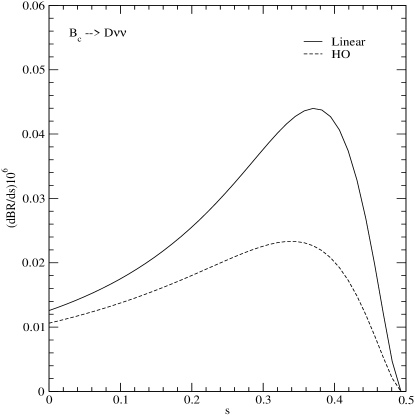
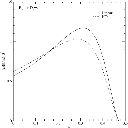
Figure 4: Differential branching ratios for $B_{c}\to D\sum\nu_{\ell}\bar{\nu_{\ell}}$ (upper panel) and $B_{c}\to D_{s}\sum\nu_{\ell}\bar{\nu_{\ell}}$ (lower panel) obtained from the linear (solid line) and HO (dashed line) potential parameters.

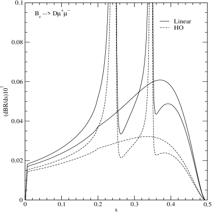
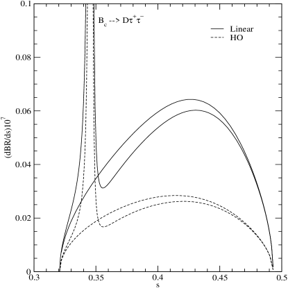
Figure 5: Differential branching ratios for $B_{c}\to D\mu^{+}\mu^{-}$ (upper panel) and $B_{c}\to D\tau^{+}\tau^{-}$ (lower panel) obtained from the linear (solid line) and HO (dashed line) potential parameters. The curves with (without) resonant shapes represent the results with (without) the LD contributions.

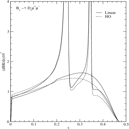
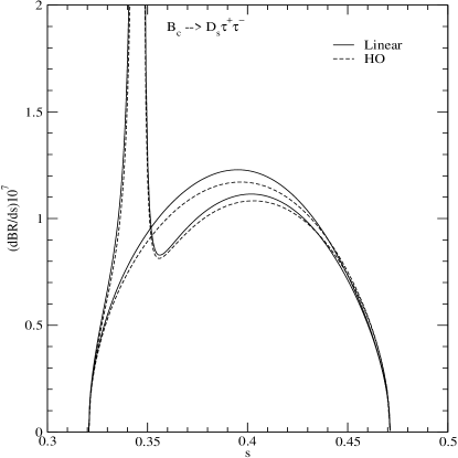
Figure 6: Differential branching ratios for $B_{c}\to D_{s}\mu^{+}\mu^{-}$ (upper panel) and $B_{c}\to D_{s}\tau^{+}\tau^{-}$ (lower panel) obtained from the linear (solid line) and HO (dashed line) potential parameters.

We show our results for the differential branching ratios for $B_{c}\to(D,D_{s})\sum\nu_{\ell}\bar{\nu}_{\ell}$ in Fig. 4, $B_{c}\to D\ell^{+}\ell^{-}$ in Fig. 5, and $B_{c}\to D_{s}\ell^{+}\ell^{-}$ in Fig. 6, respectively. The solid (dashed) line represents the result obtained from the linear (HO) potential parameters. For the $B_{c}\to(D,D_{s})\ell^{+}\ell^{-}$ transitions in Figs. 5 and 6, the curves with (without) resonant shapes represent the results with (without) the LD contribution to $C^{\rm eff}_{9}$. Although the form factor $f_{-}(q^{2})$ does not contribute to the branching ratio in the massless lepton ($\ell=e$ or $\mu$) decay, it is necessary for the heavy $\tau$ decay process. As one can see from Figs. 5 and 6, the LD contributions clearly overwhelm the branching ratios near $J/\psi(1S)$ and $\psi^{\prime}(2S)$ peaks, however, suitable $\ell^{+}\ell^{-}$ invariant mass cuts can separate the LD contribution from the SD one away from these peaks. This divides the spectrum into two distinct regions Hew ; AGM : (i) low-dilepton mass, $4m^{2}_{\ell}\leq q^{2}\leq M^{2}_{J/\psi}-\delta$, and (ii) high-dilepton mass, $M^{2}_{\psi^{\prime}}+\delta\leq q^{2}\leq q^{2}_{\rm max}$, where $\delta$ is to be matched to an experimental cut.

Our predictions for the nonresonant branching ratios obtained from the linear and the HO potential parameters are summarized in Table 4 and compared with other theoretical predictions Faessler ; Geng ; Azizi within the SM. Since the amplitude $B_{c}\to(D,D_{s})\ell^{+}\ell^{-}$ is regular at $q^{2}=0$, the transitions $B_{c}\to(D,D_{s})e^{+}e^{-}$ and $B_{c}\to(D,D_{s})\mu^{+}\mu^{-}$ have almost the same decay rates, i.e. insensitive to the mass of the light lepton. The branching ratios with the LD contributions for $B_{c}\to(D,D_{s})\ell^{+}\ell^{-}$ $(\ell=\mu,\tau)$ obtained from the linear (HO) potential parameters are also presented in Table 5 for low- and high-dilepton mass regions of $q^{2}$.

Table 4: Nonresonant branching ratios (in units of $10^{-8}$) for $B_{c}\to(D,D_{s})(\nu_{\ell}\bar{\nu}_{\ell})$ and $B_{c}\to(D,D_{s})(\ell^{+}\ell^{-})$ transitions compared with other theoretical model predictions within the SM.

Mode	Linear	HO	Faessler	Geng	Azizi
$B_{c}\to D\sum\nu_{\ell}\bar{\nu}_{\ell}$	1.31	0.81	3.28	2.74	$(3.38\pm 0.71)$
$B_{c}\to D_{s}\sum\nu_{\ell}\bar{\nu}_{\ell}$	39	37	73	92	$(49\pm 12)$
$B_{c}\to D\mu^{+}\mu^{-}$	0.18	0.11	0.44	0.40	$(0.31\pm 0.06)$
$B_{c}\to D_{s}\mu^{+}\mu^{-}$	5.4	5.1	9.7	13.3	$(6.1\pm 1.5)$
$B_{c}\to D\tau^{+}\tau^{-}$	0.08	0.04	0.11	0.12	$(0.13\pm 0.03)$
$B_{c}\to D_{s}\tau^{+}\tau^{-}$	1.4	1.3	2.2	3.7	$(2.3\pm 0.5)$

Table 5: Branching ratios with the LD contributions for $B_{c}\to(D,D_{s})\ell^{+}\ell^{-}$ for low and high dilepton mass regions of $q^{2}$ [GeV²] obtained from the linear (HO) potential parameters.

Mode	$4m^{2}_{\ell}\leq q^{2}\leq 8.5$	$13.8\leq q^{2}\leq q^{2}_{\rm max}$
$B_{c}\to D\mu^{+}\mu^{-}$	$6.56\;(4.98)\times 10^{-10}$	$5.00\;(2.38)\times 10^{-10}$
$B_{c}\to D\tau^{+}\tau^{-}$		$6.68\;(3.01)\times 10^{-10}$
$B_{c}\to D_{s}\mu^{+}\mu^{-}$	$2.68\;(2.75)\times 10^{-8}$	$0.86\;(0.69)\times 10^{-8}$
$B_{c}\to D_{s}\tau^{+}\tau^{-}$		$1.09\;(1.07)\times 10^{-8}$

In Figs. 7 and 8, we show the LPAs for $B\to D\ell^{+}\ell^{-}$ and $B\to D_{s}\ell^{+}\ell^{-}$ ($\ell=\mu,\tau$) as a function of $s$, respectively, obtained from the linear (solid line) and HO (dashed line) potential parameters. The curves with (without) resonant shapes represent the results with (without) the LD contributions. In both figures, the LPAs become zero at the end point regions of $s$. However, we note that if $m_{\ell}=0$, the LPAs are not zero at the end points. As in the case of the $B\to K\mu^{+}\mu^{-}$ decay where $P_{L}\simeq-1$ away from the end point regions CJK ; GK ; MN ; HQ , the LPAs away from the end point regions are close to $-1$ for both $B_{c}\to D\mu^{+}\mu^{-}$ and $B_{c}\to D_{s}\mu^{+}\mu^{-}$ transitions. In fact, the $P_{L}$ for the muon decay is insensitive to the form factors, e.g. our $P_{L}$ away from the end point regions is well approximated by HQ

$$P_{L}\simeq 2\frac{C_{10}{\rm Re}C^{\rm eff}_{9}}{|C^{\rm eff}_{9}|^{2}+|C_{10}|^{2}}\simeq-1,$$ (23)

in the limit of $C^{\rm eff}_{7}\to 0$ from Eq. (12). It also shows that the LPA for the $\mu$ dilepton channel is insensitive to the little variation of $C^{\rm eff}_{7}$ as expected. On the other hand, the LPA for the $\tau$ dilepton channel is somewhat sensitive to the form factors.

The averaged values of $P_{L}$ without the LD contributions obtained from the linear (HO) potential parameters are $\langle P_{L}(B_{c}\to D\mu^{+}\mu^{-})\rangle=-0.99\;(-0.99)$, $\langle P_{L}(B_{c}\to D\tau^{+}\tau^{-})=-0.16\;(-0.15)$, $\langle P_{L}(B_{c}\to D_{s}\mu^{+}\mu^{-})\rangle=-0.98\;(-0.98)$ and $\langle P_{L}(B_{c}\to D_{s}\tau^{+}\tau^{-})=-0.14\;(-0.12)$, respectively.

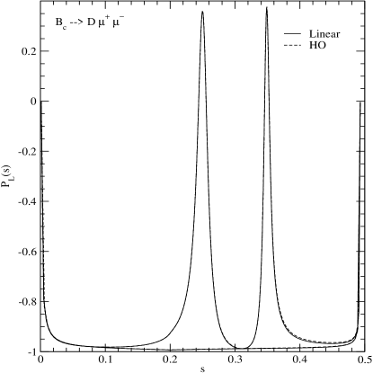
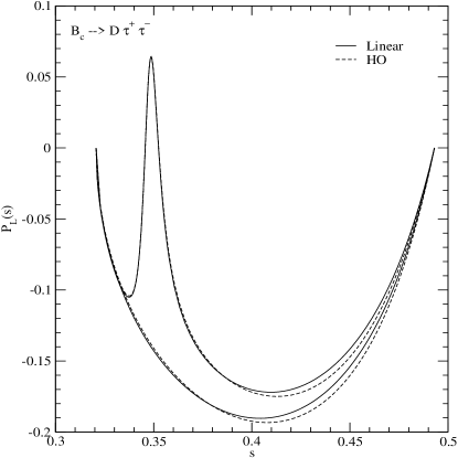
Figure 7: Longitudinal lepton polarization asymmetries for $B_{c}\to D\mu^{+}\mu^{-}$(upper panel) and $B_{c}\to D\tau^{+}\tau^{-}$(lower panel) obtained from the linear (solid line) and HO (dashed line) potential parameters.

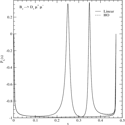
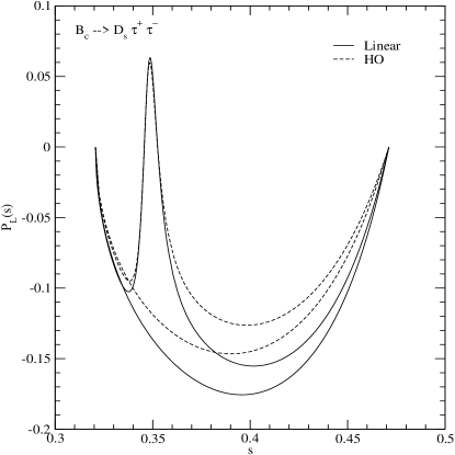
Figure 8: Longitudinal lepton polarization asymmetries for $B_{c}\to D_{s}\mu^{+}\mu^{-}$(upper panel) and $B_{c}\to D_{s}\tau^{+}\tau^{-}$(lower panel) obtained from the linear (solid line) and HO (dashed line) potential parameters.

V Summary and Discussion

In this work, we investigated the exclusive rare semileptonic $B_{c}\to(D,D_{s})\nu_{\ell}\bar{\nu_{\ell}}$ and $B_{c}\to(D,D_{s})\ell^{+}\ell^{-}$ ($\ell=e,\mu,\tau$) decays within the SM, using our LFQM constrained by the variational principle for the QCD motivated effective Hamiltonian with the linear ( or HO) plus Coulomb interaction. Our model parameters obtained from the variational principle uniquely determine the physical quantities related to the above processes. This approach can establish the broader applicability of our LFQM to the wider range of hadronic phenomena. For instance, our LFQM has been tested extensively in the spacelike processes CJ1 as well as in the timelike exclusive processes such as semileptonic CJ_PLB1 ; JC_E ; CJBc , rare semileptonic CJK , radiative ChoiRD , and nonleptonic two-body CJNRD decays of pseudoscalar and vector mesons.

The weak form factors $f_{\pm}(q^{2})$ and $f_{T}(q^{2})$ for the rare semileptonic decays between two pseudoscalar mesons are obtained in the $q^{+}=0$ frame ($q^{2}=-{\bf q}^{2}_{\perp}<0$) and then analytically continued to the timelike region by changing ${\bf q}^{2}_{\perp}$ to $-q^{2}$ in the form factor. The covariance (i.e., frame independence) of our model has been checked by performing the LF calculation in the $q^{+}=0$ frame in parallel with the manifestly covariant calculation using the exactly solvable covariant fermion field theory model in $(3+1)$-dimensions. While the form factors $f_{+}(q^{2})$ and $f_{T}(q^{2})$ are immune to the zero modes, the form factor $f_{-}(q^{2})$ is not free from the zero mode. Our numerical results show that the zero-mode contribution to the form factor $f_{-}(q^{2})$ amounts to $7\%\sim 15\%$ for both $B_{c}\to D$ and $B_{c}\to D_{s}$ decays.

Using the solutions of the weak form factors obtained from the $q^{+}=0$ frame, we calculated the branching ratios for $B_{c}\to(D,D_{s})\nu_{\ell}\bar{\nu_{\ell}}$ and $B_{c}\to(D,D_{s})\ell^{+}\ell^{-}$ and the LPAs for $B_{c}\to(D,D_{s})\ell^{+}\ell^{-}$ including both short- and long-distance contributions from the QCD Wilson coefficients. Our numerical results for the nonresonant branching ratios for $B_{c}\to D(D_{s})\sum\nu_{\ell}\bar{\nu_{\ell}}$ and $B_{c}\to D(D_{s})\ell^{+}\ell^{-}$ are in the order of $10^{-8}\;(10^{-7})$ and $10^{-9}\;(10^{-8})$, respectively. The averaged values of the LPAs obtained from the linear (HO) potential parameters are found to be $-0.99\;(-0.99)$ for $B_{c}\to D\mu^{+}\mu^{-}$ and $-0.16\;(-0.15)$ for $B_{c}\to D\tau^{+}\tau^{-}$, and $-0.98\;(-0.98)$ for $B_{c}\to D_{s}\mu^{+}\mu^{-}$ and $-0.14\;(-0.12)$ for $B_{c}\to D_{s}\tau^{+}\tau^{-}$, respectively. These polarization asymmetries provide valuable information on the flavor changing loop effects in the SM. Although the $q^{2}$ dependent behaviors of our form factors for the $B_{c}\to D_{(d,s)}$ transitions are not much different from those of other theoretical predictions Faessler ; Geng ; Azizi , our results for the decay rates are slightly less than those of Refs. Faessler ; Geng ; Azizi . This difference essentially comes from the different values of the form factors at the maximum recoil point and may be tested by future experiments. The decay rates for the $B_{c}\to D\ell^{+}\ell^{-}$ and the LPAs for the $B_{c}\to D_{s}\tau^{+}\tau^{-}$ are also quite sensitive to the choice of potential within our LFQM. From the future experimental data on these sensitive processes, one may obtain more realistic information on the potential between quark and antiquark in the heavy meson system.

Appendix A LF covariance of tensor form factor $f_{T}(q^{2})$

In the solvable model, based on the covariant Bethe-Salpeter (BS) model of ($3+1$)-dimensional fermion field theory BCJ01 ; MF ; Jaus99 , the matrix element $J^{\mu}_{T}$ of the tensor current (see Eq. (5)) is given by

$$J^{\mu}_{T}=ig_{1}g_{2}\Lambda^{2}_{1}\Lambda^{2}_{2}\int\frac{d^{4}k}{(2\pi)^{4}}\frac{S^{\mu}_{T}}{N_{\Lambda_{1}}N_{1}N_{k}N_{2}N_{\Lambda_{2}}},$$ (24)

where $g_{1}$ and $g_{2}$ are the normalization factors which can be fixed by requiring both charge form factors of pseudoscalar mesons to be unity at zero momentum transfer, respectively. The denominators in Eq. (24), are given by

$$N_{k} = k^{2}-m^{2}+i\epsilon,\;N_{j}=p_{j}^{2}-{m_{j}}^{2}+i\epsilon,$$

$$N_{\Lambda_{j}} = p_{j}^{2}-{\Lambda_{j}}^{2}+i\epsilon\;(j=1,2),$$ (25)

where $m_{1}$, $m$, and $m_{2}$ are the masses of the constituents carrying the intermediate four-momenta $p_{1}=P_{1}-k$, $k$, and $p_{2}=P_{2}-k$, respectively. $\Lambda_{1}$ and $\Lambda_{2}$ play the role of momentum cut-offs similar to the Pauli-Villars regularization BCJ01 . The trace term $S^{\mu}_{T}$ is given by

$$S^{\mu}_{T} = {\rm Tr}[\gamma_{5}(\not\!p_{1}+m_{1})i\sigma^{\mu\nu}q_{\nu}(\not\!p_{2}+m_{2})\gamma_{5}(-\not\!k+m)]$$ (26)

$$= -4\{p^{\mu}_{1}[m(p_{2}\cdot q)+m_{2}(k\cdot q)]-p^{\mu}_{2}[m(p_{1}\cdot q)$$

$$+m_{1}(k\cdot q)]+k^{\mu}[m_{1}(p_{2}\cdot q)-m_{2}(p_{1}\cdot q)]\}.$$

Following the same procedure as in CJBc for the calculation of the form factors $f_{\pm}(q^{2})$, we obtain the manifestly covariant form factor $f_{T}(q^{2})$ as follows:

$$f^{\rm Cov}_{T}(q^{2}) = \frac{N(M_{1}+M_{2})}{8\pi^{2}(\Lambda^{2}_{1}-m^{2}_{1})(\Lambda^{2}_{2}-m^{2}_{2})}\int^{1}_{0}dx\int^{1-x}_{0}dy$$ (27)

$$\times[xm_{1}+ym_{2}+(1-x-y)m]C,$$

where $N=g_{1}g_{2}\Lambda^{2}_{1}\Lambda^{2}_{2}$ and $C$ is given by Eq. (14) of Ref. CJBc .

Performing the LF calculation of Eq. (24) in the $q^{+}=0$ frame, we use the plus component of the currents to obtain the form factor $f_{T}(q^{2})$, i.e.,

$$f^{\rm LF}_{T}(q^{2})=(M_{1}+M_{2})\frac{J^{+}_{T}}{2q^{2}P^{+}_{1}}.$$ (28)

The LF calculation for $S^{\mu}_{T}$ in (26) can be separated into the on-mass shell ( $p^{-}=p^{-}_{\rm on}$) propagating part $S^{\mu}_{\rm on}$ and the (off-mass shell) instantaneous one $S^{\mu}_{\rm inst}$ using the following identity:

$$\not\!p+m=(\not\!p_{\rm on}+m)+\frac{1}{2}\gamma^{+}(p^{-}-p^{-}_{\rm on}).$$ (29)

Then the trace term $S^{\mu}_{T}$ in Eq. (26) is given by

$$S^{\mu}_{T}=S^{\mu}_{T\rm on}+S^{\mu}_{T\rm inst},$$ (30)

where the on-mass shell propagating part $S^{\mu}_{T\rm on}$ has the same form as $S^{\mu}_{T}$ in Eq. (26) but with $p^{-}=p^{-}_{\rm on}$. The instantaneous part $S^{\mu}_{T\rm inst}$ is given by

$$S^{\mu}_{T\rm inst} = -2g^{\mu+}\Delta p^{-}_{1}[m(p_{2\rm on}\cdot q)+m_{2}(k_{\rm on}\cdot q)]$$

$$+ 2g^{\mu+}\Delta p^{-}_{2}[m(p_{1\rm on}\cdot q)+m_{1}(k_{\rm on}\cdot q)]$$

$$+ 2g^{\mu+}\Delta k^{-}[m_{2}(p_{1\rm on}\cdot q)-m_{1}(p_{2\rm on}\cdot q)],$$

where $\Delta p^{-}_{i}=p^{-}_{i}-p^{-}_{i\rm on}$. By doing the integration over $k^{-}$ in Eq. (24), one finds the two LF time-ordered contributions to the residue calculations corresponding to the two poles in $k^{-}$, the LF valence contribution defined in $0<k^{+}<P^{+}_{2}$ region and the nonvalence contribution defined in $P^{+}_{2}<k^{+}<P^{+}_{1}$ region. The nonvalence contribution in the $q^{+}>0$ frame corresponds to the zero mode (if it exists) in the $q^{+}\to 0$ limit. As we have shown in CJBc ; BCJ01 , the LF valence contribution comes exclusively from the on-mass shell propagating part and the zero mode from the instantaneous part. This implies that the form factor $f_{T}(q^{2})$ is free from the zero mode since $S^{+}_{T\rm inst}=0$. The LF form factor $f^{\rm LF}_{T}(q^{2})$ is then obtained as

$$f^{\rm LF}_{T}(q^{2}) = \frac{N}{8\pi^{3}}(M_{1}+M_{2})\int^{1}_{0}\frac{dx}{(1-x)}\int d^{2}{\bf k}_{\perp}\chi_{1}(x,{\bf k}_{\perp})$$ (32)

$$\times\chi_{2}(x,{\bf k^{\prime}}_{\perp})\biggl{[}(m_{1}-m_{2})\frac{{\bf k}_{\perp}\cdot{\bf q}_{\perp}}{{\bf q}^{2}_{\perp}}+{\cal A}_{1}\biggr{]},$$

where ${\bf k^{\prime}}_{\perp}={\bf k}_{\perp}+(1-x){\bf q}_{\perp}$, ${\cal A}_{i}=(1-x)m_{i}+xm(i=1,2)$, and $q\cdot P=M^{2}_{1}-M^{2}_{2}$. The LF vertex functions $\chi_{1}$ and $\chi_{2}$ are given by

$$\chi_{1}(x,{\bf k}_{\perp}) = \frac{1}{x^{2}(M^{2}_{1}-M^{2}_{0})(M^{2}_{1}-M^{2}_{\Lambda_{1}})},$$

$$\chi_{2}(x,{\bf k^{\prime}}_{\perp}) = \frac{1}{x^{2}(M^{2}_{2}-M^{\prime 2}_{0})(M^{2}_{2}-M^{\prime 2}_{\Lambda_{2}})},$$ (33)

where

$$M^{2}_{0} = \frac{{\bf k}^{2}_{\perp}+m^{2}}{1-x}+\frac{{\bf k}^{2}_{\perp}+m^{2}_{1}}{x},$$

$$M^{\prime 2}_{0} = \frac{{\bf k^{\prime}}^{2}_{\perp}+m^{2}}{1-x}+\frac{{\bf k^{\prime}}^{2}_{\perp}+m^{2}_{2}}{x},$$ (34)

and $M^{2}_{\Lambda_{1}}=M^{2}_{0}(m_{1}\to\Lambda_{1})$, $M^{\prime 2}_{\Lambda_{2}}=M^{\prime 2}_{0}(m_{2}\to\Lambda_{2})$. We numerically confirm that our LF form factor $f^{\rm LF}_{T}(q^{2})$ is exactly the same as the manifestly covariant form factor $f^{\rm Cov}_{T}(q^{2})$. This proves that $f^{\rm LF}_{T}(q^{2})$ is immune to the zero mode.

Following the same procedure CJBc to obtain the form factors $f_{\pm}(q^{2})$ within our LFQM, the form factor $f_{T}(q^{2})$ given by Eq. (III) is obtained by the following relations:

$$\sqrt{2N}\frac{\chi_{1}(x,{\bf k}_{\perp})}{1-x} = \frac{\phi_{1}(x,{\bf k}_{\perp})}{\sqrt{{\cal A}^{2}_{1}+{\bf k}^{2}_{\perp}}},$$

$$\sqrt{2N}\frac{\chi_{2}(x,{\bf k^{\prime}}_{\perp})}{1-x} = \frac{\phi_{2}(x,{\bf k^{\prime}}_{\perp})}{\sqrt{{\cal A}^{2}_{2}+{\bf k^{\prime}}^{2}_{\perp}}}.$$ (35)

References

(1) B. Grinstein, M. B. Wise and M. J. Savage,
Nucl. Phys. B 319, 271 (1989).
(2) A. J. Buras and M. Mnz,
Phys. Rev. D 52, 186 (1995).
(3) M. Misiak, Nucl. Phys. B 393, 23 (1993);
. 439, 461(E) (1995).
(4) T. Inami and C. S. Lim, Prog. Theor. Phys. 65,
297 (1981); G. Buchalla, A. J. Buras, and M.E. Lautcnbacher,
Rev. Mod. Phys. 68, 1125 (1996).
(5) A. Ali, T. Mannel and T. Morozumi,
Phys. Lett. B 273, 505 (1991); A. Ali, Acta Phys. Pol. B
27, 3529 (1996).
(6) C. S. Kim, T. Morozumi, and A. I. Sanda,
Phys. Rev. D 56, 7240 (1997).
(7) T. M. Aliev, C. S. Kim, and M. Savci,
Phys. Lett. B 441, 410 (1998).
(8) A. Faessler, Th. Gutsche, M.A. Ivanov, J.G. Körner,
and V.E. Lyubovitskij, Eur. Phys. J. direct C 4, 18 (2002).
(9) C.Q. Geng, C.W. Hwang, and C.C. Liu, Phys. Rev. D 65, 094037 (2002).
(10) K. Azizi and R. Khosravi, Phys. Rev. D 78, 036005 (2008).
(11) U.O. Yilmaz, Phys. Rev. D 78, 055004 (2008).
(12) S. J. Brodsky, H. -C. Pauli, and S. S. Pinsky,
Phys. Rep. 301, 299 (1998).
(13) H. -M. Choi and C. -R. Ji, Phys. Rev. D 59, 074015 (1999).
(14) H.-M. Choi and C. -R. Ji, Phys. Lett. B 460, 461 (1999);
Phys. Rev. D 59, 034001 (1998).
(15) C. -R. Ji and H. -M. Choi, Phys. Lett. B 513, 330 (2001).
(16) H. -M. Choi, C. -R. Ji, and L. S. Kisslinger,
Phys. Rev. D 65, 074032 (2002).
(17) H. -M. Choi, Phys. Rev. D 75, 073016 (2007).
(18) H. -M. Choi and C. -R. Ji, Phys. Rev. D 80, 054016 (2009).
(19) H. -M. Choi and C. -R. Ji, Phys. Rev. D 80, 114003 (2009).
(20) J. L. Hewett, Phys. Rev. D 53, 4964 (1996);
F. Krger and L. M. Sehgal, Phys. Lett. B 380, 199 (1996).
(21) S. D. Drell and T. M. Yan, Phys. Rev. Lett. 24, 181 (1970);
G. West, Phys. Rev. Lett. 24, 1206 (1970).
(22) H.-M. Choi and C.-R. Ji,
Phys. Rev. D 58, 071901(R) (1998);
Phys. Rev. D 72, 013004 (2005); S. J. Brodsky and D. S. Hwang,
Nucl. Phys. B 543, 239 (1999); M. Burkardt, Phys. Rev. D 47, 4628 (1993);
J.P.B.C. de Melo, J.H.O. Sales, T. Frederico, and P.U. Sauer,
Nucl. Phys. A 631, 574c (1998).
(23) D. Melikhov and N. Nikitin,
Phys. Rev. D 57, 6814 (1998).
(24) C. Q. Geng and C. P. Kao, Phys. Rev. D 54, 5636 (1996).
(25) C. Amsler et al.(Particle Data Group),
Phys. Lett. B 667, 1 (2008).
(26) A. Ali, G. F. Guidice, and T. Mannel,
Z. Phys. C 67, 417 (1995).
(27) W. Roberts, Phys. Rev. D 54, 863 (1996);
G. Burdman, Phys. Rev. D 52, 6400 (1995).
(28) B.L.G. Bakker, H.-M. Choi, and C.-R. Ji,
Phys. Rev. D 63, 074014 (2001); Phys. Rev. D 65, 116001 (2002);
Phys. Rev. D 67, 113007 (2003).
(29) J.P.B.C. de Melo and T. Frederico,
Phys. Rev. C 55, 2043 (1997); J.P.B.C. de Melo, T. Frederico, E. Pace, and
G. Salme, Phys. Rev. D 73, 074013 (2006).