Chapter 1 $B$ physics in the LHC era

Gino Isidori
INFN, Laboratori Nazionali di Frascati, I-00044 Frascati, Italy

Institute for Advanced Study, T. U. München, D-80333 München, Germany

1 Introduction

In the last few years there has been a great experimental progress in quark flavour physics. The validity of the Standard Model (SM) has been strongly reinforced by a series of challenging experimental tests in $B$, $D$, and $K$ decays. All the relevant SM parameters controlling quark-flavour dynamics (the quark masses and the angles of the Cabibbo-Kobayashi-Maskawa matrix [2, 3] have been determined with good accuracy. More important, several suppressed observables (such as $\Delta m_{B_{d}}$, $\Delta m_{B_{s}}$, ${\cal A}^{{}_{\rm CP}}_{K\Psi}$, $B\to X_{s}\gamma$, $\epsilon_{K}$, …) potentially sensitive to physics beyond the SM have been measured with good accuracy, showing no deviations from the SM. The situation is somehow similar to the flavour-conserving electroweak precision observables after LEP: the SM works very well and genuine one-loop electroweak effects have been tested with relative accuracy in the $10\%$–$30\%$ range. Similarly to the case of electroweak observables, also in the quark flavour sector non-standard effects can only appear as small corrections to the leading SM contribution.

Despite the success of the SM in electroweak and quark-flavour physics, we have also clear indications that this theory is not complete: the phenomenon of neutrino oscillations and the evidence for dark matter cannot be explained within the SM. The SM is also affected by a serious theoretical problem because of the instability of the Higgs sector under quantum corrections. We have not yet enough information to unambiguously determine how the SM Lagrangian should be modified; however, most realistic proposals point toward the existence of new degrees of freedom in the TeV range, possibly accessible at the high-$p_{T}$ experiments at the LHC.

Assuming that the SM is not a complete theory, the precise tests of flavour dynamics performed so far imply a series of challenging constraints about the new theory: if there are new degrees of freedom at the TeV scale, present data tell us that they must posses a highly non-generic flavour structure. This structure is far from being established and its deeper investigation is the main goal of continuing high-precision flavour-physics in the LHC era. In these lectures we focus on the interest and potential impact of future measurements in the $B$-meson system in this perspective.

The lectures are organized as follows: in the first lecture we briefly recall the main features of flavour physics within the SM. We also address in general terms the so-called flavour problem, namely the challenge to any SM extension posed by the success of the SM in flavour physics. In the second lecture we analyse in some detail the SM predictions for some of the most interesting $B$ physics observables to be measured in the LHC era. In the last lecture we analyse flavour physics in various realistic beyond-the-SM scenarios, discussing how they can be tested by future experiments.

The presentation of these lectures is somehow original, but all the material can be found, often with more details, in various set of lectures [4] and review articles [5, 6, 7] present in the recent literature.

2 Flavour physics within the SM and the flavour problem

2.1 The flavour sector of the SM

The Standard Model (SM) Lagrangian can be divided into two main parts, the gauge and the Higgs (or symmetry breaking) sector. The gauge sector is extremely simple and highly symmetric: it is completely specified by the local symmetry ${\mathcal{G}}^{\rm SM}_{\rm local}=SU(3)_{C}\times SU(2)_{L}\times U(1)_{Y}$ and by the fermion content,

$${\cal L}^{\rm SM}_{\rm gauge} = \sum_{i=1\ldots 3}\ \sum_{\psi=Q^{i}_{L}\ldots E^{i}_{R}}{\bar{\psi}}iD\!\!\!\!/~{}\psi$$ (1)

$$-\frac{1}{4}\sum_{a=1\ldots 8}G^{a}_{\mu\nu}G^{a}_{\mu\nu}-\frac{1}{4}\sum_{a=1\ldots 3}W^{a}_{\mu\nu}W^{a}_{\mu\nu}-\frac{1}{4}B_{\mu\nu}B_{\mu\nu}~{}.$$

The fermion content consist of five fields with different quantum numbers under the gauge group.

$$Q^{i}_{L}(3,2)_{+1/6}~{},\ \ U^{i}_{R}(3,1)_{+2/3}~{},\ \ D^{i}_{R}(3,1)_{-1/3}~{},\ \ L^{i}_{L}(1,2)_{-1/2}~{},\ \ E^{i}_{R}(1,1)_{-1}~{},$$ (2)

each of them appearing in three different replica or flavours ($i=1,2,3$).

This structure give rise to a large global flavour symmetry of ${\cal L}^{\rm SM}_{\rm gauge}$. Both the local and the global symmetries of ${\cal L}^{\rm SM}_{\rm gauge}$ are broken with the introduction of a $SU(2)_{L}$ scalar doublet $\phi$, or the Higgs field. The local symmetry is spontaneously broken by the vacuum expectation value of the Higgs field, $\langle\phi\rangle=v=(2\sqrt{2}G_{F})^{-1/2}\approx 174$ GeV, while the global flavour symmetry is explicitly broken by the Yukawa interaction of $\phi$ with the fermion fields:

$$-{\cal L}^{\rm SM}_{\rm Yukawa}=Y_{d}^{ij}{\bar{Q}}^{i}_{L}\phi D^{j}_{R}+Y_{u}^{ij}{\bar{Q}}^{i}_{L}\tilde{\phi}U^{j}_{R}+Y_{e}^{ij}{\bar{L}}_{L}^{i}\phi E_{R}^{j}+{\rm h.c.}\qquad(\tilde{\phi}=i\tau_{2}\phi^{\dagger})~{}.$$ (3)

The large global flavour symmetry of ${\cal L}^{\rm SM}_{\rm gauge}$, corresponding to the independent unitary rotations in flavour space of the five fermion fields in Eq. (2), is a $U(3)^{5}$ group. This can be decomposed as follows:

$${\mathcal{G}}_{\rm flavour}=U(3)^{5}\times{\mathcal{G}}_{q}\times{\mathcal{G}}_{\ell}~{},$$ (4)

where

$${\mathcal{G}}_{q}={SU}(3)_{Q_{L}}\times{SU}(3)_{U_{R}}\times{SU}(3)_{D_{R}},\qquad{\mathcal{G}}_{\ell}={SU}(3)_{L_{L}}\otimes{SU}(3)_{E_{R}}~{}.$$ (5)

Three of the five $U(1)$ subgroups can be identified with the total barion and lepton number, which are not broken by ${\cal L}_{\rm Yukawa}$, and the weak hypercharge, which is gauged and broken only spontaneously by $\langle\phi\rangle\not=0$. The subgroups controlling flavour-changing dynamics and flavour non-universality are the non-Abelian groups ${\mathcal{G}}_{q}$ and ${\mathcal{G}}_{\ell}$, which are explicitly broken by $Y_{d,u,e}$ not being proportional to the identity matrix.

The diagonalization of each Yukawa coupling requires, in general, two independent unitary matrices, $V_{L}YV^{\dagger}_{R}={\rm diag}(y_{1},y_{2},y_{3})$. In the lepton sector the invariance of ${\cal L}^{\rm SM}_{\rm gauge}$ under ${\mathcal{G}}_{\ell}$ allows us to freely choose the two matrices necessary to diagonalize $Y_{e}$ without breaking gauge invariance, or without observable consequences. This is not the case in the quark sector, where we can freely choose only three of the four unitary matrices necessary to diagonalize both $Y_{d}$ and $Y_{u}$. Choosing the basis where $Y_{d}$ is diagonal (and eliminating the right-handed diagonalization matrix of $Y_{u}$) we can write

$$Y_{d}=\lambda_{d}~{},\qquad Y_{u}=V^{\dagger}\lambda_{u}~{},$$ (6)

where

$$\lambda_{d}={\rm diag}(y_{d},y_{s},y_{b})~{},\ \ \ \lambda_{u}={\rm diag}(y_{u},y_{c},y_{t})~{},\qquad y_{q}=\frac{m_{q}}{v}~{}.$$ (7)

Alternatively we could choose a gauge-invariant basis where $Y_{d}=V\lambda_{d}$ and $Y_{u}=\lambda_{u}$. Since the flavour symmetry do not allow the diagonalization from the left of both $Y_{d}$ and $Y_{u}$, in both cases we are left with a non-trivial unitary mixing matrix, $V$, which is nothing but the Cabibbo-Kobayashi-Maskawa (CKM) mixing matrix [2, 3].

A generic unitary $3\times 3$ [$N\times N$] complex unitary matrix depends on three [$N(N-1)/2$] real rotational angles and six [$N(N+1)/2$] complex phases. Having chosen a quark basis where the $Y_{d}$ and $Y_{u}$ have the form in (6) leaves us with a residual invariance under the flavour group which allows us to eliminate five of the six complex phases in $V$ (the relative phases of the various quark fields). As a result, the physical parameters in $V$ are four: three real angles and one complex CP-violating phase. The full set of parameters controlling the breaking of the quark flavour symmetry in the SM is composed by the six quark masses in $\lambda_{u,d}$ and the four parameters of $V$.

For practical purposes it is often convenient to work in the mass eigenstate basis of both up- and and down-type quarks. This can be achieved rotating independently the up and down components of the quark doublet $Q_{L}$, or moving the CKM matrix from the Yukawa sector to the charged weak current in ${\cal L}^{\rm SM}_{\rm gauge}$:

$$\left.J_{W}^{\mu}\right|_{\rm quarks}=\bar{u}^{i}_{L}\gamma^{\mu}d^{i}_{L}\quad\stackrel{{\scriptstyle u,d~{}{\rm mass-basis}}}{{\longrightarrow}}\quad\bar{u}^{i}_{L}V_{ij}\gamma^{\mu}d^{j}_{L}~{}.$$ (8)

However, it must be stressed that $V$ originates from the Yukawa sector (in particular by the miss-alignment of $Y_{u}$ and $Y_{d}$ in the ${SU}(3)_{Q_{L}}$ subgroup of ${\mathcal{G}}_{q}$): in absence of Yukawa couplings we can always set $V_{ij}=\delta_{ij}$.

To summarize, quark flavour physics within the SM is characterized by a large flavour symmetry, ${\mathcal{G}}_{q}$, defined by the gauge sector, whose only breaking sources are the two Yukawa couplings $Y_{d}$ and $Y_{u}$. The CKM matrix arises by the miss-alignment of $Y_{u}$ and $Y_{d}$ in flavour space.

2.2 Some properties of the CKM matrix

The standard parametrization of the CKM matrix [8] in terms of three rotational angles ($\theta_{ij}$) and one complex phase ($\delta$) is

$$V = \left(\begin{array}[]{ccc}V_{ud}&V_{us}&V_{ub}\\ V_{cd}&V_{cs}&V_{cb}\\ V_{td}&V_{ts}&V_{tb}\end{array}\right)$$ (12)

$$= \left(\begin{array}[]{ccc}c_{12}c_{13}&s_{12}c_{13}&s_{13}e^{-i\delta}\\ -s_{12}c_{23}-c_{12}s_{23}s_{13}e^{i\delta}&c_{12}c_{23}-s_{12}s_{23}s_{13}e^{i\delta}&s_{23}c_{13}\\ s_{12}s_{23}-c_{12}c_{23}s_{13}e^{i\delta}&-s_{23}c_{12}-s_{12}c_{23}s_{13}e^{i\delta}&c_{23}c_{13}\end{array}\right)~{},$$ (16)

where $c_{ij}=\cos\theta_{ij}$ and $s_{ij}=\sin\theta_{ij}$ ($i,j=1,2,3$).

The off-diagonal elements of the CKM matrix show a strongly hierarchical pattern: $|V_{us}|$ and $|V_{cd}|$ are close to $0.22$, the elements $|V_{cb}|$ and $|V_{ts}|$ are of order $4\times 10^{-2}$ whereas $|V_{ub}|$ and $|V_{td}|$ are of order $5\times 10^{-3}$. The Wolfenstein parametrization, namely the expansion of the CKM matrix elements in powers of the small parameter $\lambda\doteq|V_{us}|\approx 0.22$, is a convenient way to exhibit this hierarchy in a more explicit way [9]:

$$V=\left(\begin{array}[]{ccc}1-{\lambda^{2}\over 2}&\lambda&A\lambda^{3}(\varrho-i\eta)\\ -\lambda&1-{\lambda^{2}\over 2}&A\lambda^{2}\\ A\lambda^{3}(1-\varrho-i\eta)&-A\lambda^{2}&1\end{array}\right)+{\cal{O}}(\lambda^{4})~{},$$ (17)

where $A$, $\varrho$, and $\eta$ are free parameters of order 1. Because of the smallness of $\lambda$ and the fact that for each element the expansion parameter is actually $\lambda^{2}$, this is a rapidly converging expansion.

The Wolfenstein parametrization is certainly more transparent than the standard parametrization. However, if one requires sufficient level of accuracy, the terms of ${\cal{O}}(\lambda^{4})$ and ${\cal{O}}(\lambda^{5})$ have to be included in phenomenological applications. This can be achieved in many different ways, according to the convention adopted. The simplest (and nowadays commonly adopted) choice is obtained defining the parameters $\{\lambda,A,\varrho,\eta\}$ in terms of the angles of the exact parametrization in Eq. (16) as follows:

$$\lambda\doteq s_{12}~{},\qquad A\lambda^{2}\doteq s_{23}~{},\qquad A\lambda^{3}(\varrho-i\eta)\doteq s_{13}e^{-i\delta}~{}.$$ (18)

The change of variables $\{s_{ij},\delta\}\to\{\lambda,A,\varrho,\eta\}$ in Eq. (16) leads to an exact parametrization of the CKM matrix in terms of the Wolfenstein parameters. Expanding this expression up to ${\cal{O}}(\lambda^{5})$ leads to

$$\left(\begin{array}[]{ccc}1-\frac{1}{2}\lambda^{2}-\frac{1}{8}\lambda^{4}&\lambda+{\cal{O}}(\lambda^{7})&A\lambda^{3}(\varrho-i\eta)\\ -\lambda+\frac{1}{2}A^{2}\lambda^{5}[1-2(\varrho+i\eta)]&1-\frac{1}{2}\lambda^{2}-\frac{1}{8}\lambda^{4}(1+4A^{2})&A\lambda^{2}+{\cal{O}}(\lambda^{8})\\ A\lambda^{3}(1-\bar{\varrho}-i\bar{\eta})&\!\!\!\!\!-A\lambda^{2}+\frac{1}{2}A\lambda^{4}[1-2(\varrho+i\eta)]&1-\frac{1}{2}A^{2}\lambda^{4}\end{array}\right)$$ (19)

where

$$\bar{\varrho}=\varrho(1-\frac{\lambda^{2}}{2})+{\cal O}(\lambda^{4})~{},\qquad\bar{\eta}=\eta(1-\frac{\lambda^{2}}{2})+{\cal O}(\lambda^{4})~{}.$$ (20)

The advantage of this generalization of the Wolfenstein parametrization is the absence of relevant corrections to $V_{us}$, $V_{cd}$, $V_{ub}$ and $V_{cb}$, and a simple change in $V_{td}$, which facilitate the implementation of experimental constraints.

The unitarity of the CKM matrix implies the following relations between its elements:

$${\bf I)}\quad\sum_{k=1\ldots 3}V_{ik}^{*}V_{ki}=1~{},\quad\qquad{\bf II)}\quad\sum_{k=1\ldots 3}V_{ik}^{*}V_{kj\not=i}~{}.$$ (21)

These relations are a distinctive feature of the SM, where the CKM matrix is the only source of quark flavour mixing. Their experimental verification is therefore a useful tool to set bounds, or possibly reveal, new sources of flavour symmetry breaking. Among the relations of type II, the one obtained for $i=1$ and $j=3$, namely

$$V_{ud}V_{ub}^{*}+V_{cd}V_{cb}^{*}+V_{td}V_{tb}^{*}=0$$ (22)

$${\rm or}\qquad\frac{V_{ud}V_{ub}^{*}}{V_{cd}V_{cb}^{*}}+\frac{V_{td}V_{tb}^{*}}{V_{cd}V_{cb}^{*}}+1=0\qquad\leftrightarrow\qquad[\bar{\varrho}+i\bar{\eta}]+[(1-\bar{\varrho})-i\bar{\eta}]+1=0~{},$$

is particularly interesting since it involves the sum of three terms all of the same order in $\lambda$ and is usually represented as a unitarity triangle in the complex plane, as shown in Fig. 1. It is worth to stress that Eq. (22) is invariant under any phase transformation of the quark fields. Under such transformations the triangle in Fig. 1 is rotated in the complex plane, but its angles and the sides remain unchanged. Both angles and sides of the unitary triangle are indeed observable quantities which can be measured in suitable experiments.

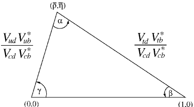
Figure 1: The CKM unitarity triangle.

2.3 Present status of CKM fits

The values of $|V_{us}|$ and $|V_{cb}|$, or $\lambda$ and $A$ in the parametrization (19), are determined with good accuracy from $K\to\pi\ell\nu$ and $B\to X_{c}\ell\nu$ decays, respectively. According to the recent analysis in Ref. [5], their numerical values are

$$\lambda=0.2259\pm 0.0009~{},\qquad A=0.802\pm 0.015~{}.$$ (23)

Using these results, all the other constraints on the elements of the CKM matrix can be expressed as constraints on $\bar{\varrho}$ and $\bar{\eta}$ (or constraints on the CKM unitarity triangle in Fig. 1). The list of the most sensitive observables used to determine $\bar{\varrho}$ and $\bar{\eta}$ in the SM includes:

• The rates of inclusive and exclusive charmless semileptonic $B$ decays, which depend on $|V_{ub}|$ and provide a constraint on $\bar{\varrho}^{2}+\bar{\eta}^{2}$.

• The time-dependent CP asymmetry in $B\to\psi K_{S}$ decays (${\cal A}^{{}_{\rm CP}}_{K\Psi}$), which depends on the phase of the $B_{d}$–$\bar{B}_{d}$ mixing amplitude relative to the decay amplitude (see Sect. 3.2). Within the SM this translates into a constraint on $\sin 2\beta$.

• The rates of various $B\to DK$ decays, which provide constraints on the angle $\gamma$ (see Sect. 3.3.2).

• The rates of various $B\to\pi\pi,\rho\pi,\rho\rho$ decays, which constrain $\alpha=\pi-\beta-\gamma$.

• The ratio between the mass splittings in the neutral $B$ and $B_{s}$ systems, which depends on $|V_{td}/V_{ts}|^{2}\propto[(1-\bar{\varrho})^{2}+\bar{\eta}^{2}]$.

• The indirect CP violating parameter of the kaon system ($\epsilon_{K}$), which determines and hyperbola in the $\bar{\varrho}$ and $\bar{\eta}$ plane (see Ref. [5] for more details).

The resulting constraints are shown in Fig. 2. As can be seen, they are all consistent with a unique value of $\bar{\varrho}$ and $\bar{\eta}$ [5]:

$$\rho=+0.158\pm 0.021~{},\qquad\eta=+0.343\pm 0.013~{}.$$ (24)

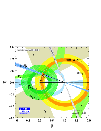
Figure 2: Allowed region in the $\bar{\varrho},\bar{\eta}$ plane, from [11]. Superimposed are the individual constraints from charmless semileptonic $B$ decays ($|V_{ub}|$), mass differences in the $B_{d}$ ($\Delta m_{d}$) and $B_{s}$ ($\Delta m_{s}$) systems, CP violation in the neutral kaon ($\varepsilon_{K}$) and in the $B_{d}$ systems ($\sin 2\beta$), the combined constrains on $\alpha$ and $\gamma$ from various $B$ decays.

The consistency of different constraints on the CKM unitarity triangle is a powerful consistency test of the SM in describing flavour-changing phenomena. From the plot in Fig. 2 it is quite clear, at least in a qualitative way, that there is little room for non-SM contributions in flavour changing transitions. A more quantitative evaluation of this statement is presented in the next section.

2.4 The SM as an effective theory

As anticipated in the introduction, despite the impressive phenomenological success of the SM in flavour and electroweak physics, there are various convincing arguments which motivate us to consider this model only as the low-energy limit of a more complete theory.

Assuming that the new degrees of freedom which complete the theory are heavier than the SM particles, we can integrate them out and describe physics beyond the SM in full generality by means of an effective theory approach. The SM Lagrangian becomes the renormalizable part of a more general local Lagrangian which includes an infinite tower of operators with dimension $d>4$, constructed in terms of SM fields and suppressed by inverse powers of an effective scale $\Lambda$. These operators are the residual effect of having integrated out the new heavy degrees of freedom, whose mass scale is parametrized by the effective scale $\Lambda>m_{W}$.

As we will discuss in more detail in Sect. 3.1, integrating out heavy degrees of freedom is a procedure often adopted also within the SM: it allows us to simplify the evaluation of amplitudes which involve different energy scales. This approach is indeed a generalization of the Fermi theory of weak interactions, where the dimension-six four-fermion operators describing weak decays are the results of having integrated out the $W$ field. The only difference when applying this procedure to physics beyond the SM is that in this case, as also in the original work by Fermi, we don’t know the nature of the degrees of freedom we are integrating out. This imply we are not able to determine a priori the values of the effective couplings of the higher-dimensional operators. The advantage of this approach is that it allows us to analyse all realistic extensions of the SM in terms of a limited number of parameters (the coefficients of the higher-dimensional operators). The drawback is the impossibility to establish correlations of New Physics (NP) effects at low and high energies.

Assuming for simplicity that there is a single elementary Higgs field, responsible for the $SU(2)_{L}\times U(1)_{Y}\to U(1)_{Q}$ spontaneous breaking, the Lagrangian of the SM considered as an effective theory can be written as follows

$${\cal L}_{\rm eff}={\cal L}^{\rm SM}_{\rm gauge}+{\cal L}^{\rm SM}_{\rm Higgs}+{\cal L}^{\rm SM}_{\rm Yukawa}+\Delta{\cal L}_{d>4}~{},$$ (25)

where $\Delta{\cal L}_{d>4}$ denotes the series of higher-dimensional operators invariant under the SM gauge group:

$$\Delta{\cal L}_{d>4}=~{}\sum_{d>4}~{}\sum_{n=1}^{N_{d}}~{}\frac{c^{(d)}_{n}}{\Lambda^{d-4}}{\cal O}^{(d)}_{n}({\rm SM~{}fields}).$$ (26)

If NP appears at the TeV scale, as we expect from the stabilization of the mechanism of electroweak symmetry breaking, the scale $\Lambda$ cannot exceed a few TeV. Moreover, if the underlying theory is natural (no fine-tuning in the coupling constants), we expect $c^{(d)}_{i}=O(1)$ for all the operators which are not forbidden (or suppressed) by symmetry arguments. The observation that this expectation is not fulfilled by several dimension-six operators contributing to flavour-changing processes is often denoted as the flavour problem.

If the SM Lagrangian were invariant under some flavour symmetry, this problem could easily be circumvented. For instance in the case of barion- or lepton-number violating processes, which are exact symmetries of the SM Lagrangian, we can avoid the tight experimental bounds promoting $B$ and $L$ to be exact symmetries of the new dynamics at the TeV scale. The peculiar aspects of flavour physics is that there is no exact flavour symmetry in the low-energy theory. In this case it is not sufficient to invoke a flavour symmetry for the underlying dynamics. We also need to specify how this symmetry is broken in order to describe the observed low-energy spectrum and, at the same time, be in agreement with the precise experimental tests of flavour-changing processes.

2.4.1 Bounds on the scale of New Physics from $\Delta F=2$ processes

The best way to quantify the flavour problem is obtained by looking at consistency of the tree- and loop-mediated constraints on the CKM matrix discussed in Sect. 2.3.

In first approximation we can assume that NP effects are negligible in processes which are dominated by tree-level amplitudes. Following this assumption, the values of $|V_{us}|$, $|V_{cb}|$, and $|V_{ub}|$, as well as the constraints on $\alpha$ and $\gamma$ are essentially NP free. As can be seen in Fig. 2, this implies we can determine completely the CKM matrix assuming generic NP effects in loop-mediated amplitudes. We can then use the measurements of observables which are loop-mediated within the SM to bound the couplings of effective NP operators in Eq. (26) which contribute to these observables at the tree level.

Figure 3: Box diagrams contributing to $B_{d}$-$\bar{B}_{d}$ mixing in the unitary gauge.

The loop-mediated constraints shown in Fig. 2 are those from the mixing of $B_{d}$, $B_{s}$, and $K^{0}$ with the corresponding anti-particles (generically denoted as $\Delta F=2$ amplitudes). Within the SM, these amplitudes are generated by box amplitudes of the type in Fig. 3 (and similarly for $B_{s}$, and $K^{0}$) and are affected by small hadronic uncertainties (with the exception of $\Delta m_{K}$). We will come back to the evaluation of these amplitudes in more detail in Sect. 3.2. For the moment it is sufficient to notice that the leading contribution is obtained with the top-quark running inside the loop, giving rise to the highly suppressed result

$${\cal M}_{\Delta F=2}^{\rm SM}\approx\frac{G_{F}^{2}m_{t}^{2}}{16\pi^{2}}~{}V_{3i}^{*}V_{3j}~{}\langle\bar{M}|(\bar{d}_{L}^{i}\gamma^{\mu}d_{L}^{j})^{2}|M\rangle\times F\left(\frac{m_{t}^{2}}{m_{W}^{2}}\right)\qquad[M=K^{0},B_{d},B_{s}]~{},$$ (27)

where $F$ is a loop function of order one ($i,j$ denote the flavour indexes of the meson valence quarks).

Magnitude and phase of all these mixing amplitudes have been determined with good accuracy from experiments with the exception of the CP-violating phase in $B_{s}$–$\bar{B}_{s}$ mixing. As shown in Fig. 2, in all cases where the experimental information is precise, the magnitude of the new-physics amplitude cannot exceed, in size, the SM contribution.

To translate this information into bounds on the scale of new physics, let’s consider the following set of $\Delta F=2$ dimensions-six operators

$${\cal O}_{\Delta F=2}^{ij}=(\bar{Q}_{L}^{i}\gamma^{\mu}Q_{L}^{j})^{2}~{},\qquad Q^{i}_{L}=\left(\begin{array}[]{c}u^{i}_{L}\\ d^{i}_{L}\end{array}\right)~{},$$ (28)

where $i,j$ are flavour indexes in the basis defined by Eq. (6). These operators contribute at the tree-level to the meson-antimeson mixing amplitudes. Denoting $c_{ij}$ the couplings of the non-standard operators in (28), the condition $|{\cal M}_{\Delta F=2}^{\rm NP}|<|{\cal M}_{\Delta F=2}^{\rm SM}|$ implies

$$\Lambda<\frac{3.4~{}{\rm TeV}}{|V_{3i}^{*}V_{3j}|/|c_{ij}|^{1/2}}<\left\{\begin{array}[]{l}9\times 10^{3}~{}{\rm TeV}\times|c_{21}|^{1/2}\qquad{\rm from}\quad K^{0}-\bar{K}^{0}\\ 4\times 10^{2}~{}{\rm TeV}\times|c_{31}|^{1/2}\qquad{\rm from}\quad B_{d}-\bar{B}_{d}\\ 7\times 10^{1}~{}{\rm TeV}\times|c_{32}|^{1/2}\qquad{\rm from}\quad B_{s}-\bar{B}_{s}\end{array}\right.$$ (32)

The main messages of these bounds are the following:

• New physics models with a generic flavour structure ($c_{ij}$ of order 1) at the TeV scale are ruled out. If we want to keep $\Lambda$ in the TeV range, physics beyond the SM must have a highly non-generic flavour structure.

• In the specific case of the $\Delta F=2$ operators in (28), in order to keep $\Lambda$ in the TeV range, we must find a symmetry argument such that $|c_{ij}|\mathrel{\raise 2.15277pt\hbox{$<$}\kern-7.44856pt\lower 4.0pt\hbox{{$\displaystyle\sim$}}}|V_{3i}^{*}V_{3j}|^{2}$.

The strong constraining power of $\Delta F=2$ observables is a consequence of their strong suppression within the SM. They are suppressed not only by the typical $1/(4\pi)^{2}$ factor of loop amplitudes, but also by the GIM mechanism [13] and by the hierarchy of the CKM matrix ($|V_{3i}|\ll 1$, for $i\not=3$). Reproducing a similar structure beyond the SM is a highly non-trivial task. As we will discuss in the last lecture, only in a few cases this can be implemented in a natural way.

To conclude, we stress that the good agreement of SM and experiments for $B_{d}$ and $K^{0}$ mixing does not imply that further studies of flavour physics are not interesting. On the one hand, even for $|c_{ij}|\approx|V_{3i}^{*}V_{3j}|$, which can be considered the most pessimistic case, as we will discuss in Sect. 4.1, we are presently constraining physics at the TeV scale. Therefore improving these bounds, if possible, would be extremely valuable. One the other hand, as we will discuss in the next lecture, there are various interesting observables which have not been deeply investigated yet, whose study could reveal additional key features about the flavour structure of physics beyond the SM.

3 $B$-physics phenomenology: mixing, CP violation, and rare decays

As we have seen in the previous lecture, the exploration of the mechanism of quark-flavour mixing is entered in a new era. The precise measurements of mixing-induced CP violation and tree-level allowed semileptonic transition have provided an important consistency check of the SM, and a precise determination of the Cabibbo-Kobayashi-Maskawa matrix. The next goal is to understand if there is still room for new physics or, more precisely, if there is still room for new sources of flavour symmetry breaking close to the electroweak scale. From this perspective, a few rare $B$ decays mediated by flavour-changing neutral-current (FCNC) amplitudes, and also the CP violating phase of $B_{s}$ mixing, represent a fundamental tool.

Beside the experimental sensitivity, the conditions which allow us to perform significant NP searches in rare decays can be summarized as follows: i) decay amplitude dominated by electroweak dynamics, and thus enhanced sensitivity to non-standard contributions; ii) small theoretical error within the SM, or good control of both perturbative and non-perturbative corrections. In the next section we analyze how and in which cases these two conditions can be achieved.

3.1 Theoretical tools: low-energy effective Lagrangians

The decays of $B$ mesons are processes which involve at least two different energy scales: the electroweak scale, characterized by the $W$ boson mass, which determines the flavor-changing transition at the quark level, and the scale of strong interactions $\Lambda_{\mathrm{QCD}}$, related to the hadron formation. The presence of these two widely separated scales makes the calculation of the decay amplitudes starting from the full SM Lagrangian quite complicated: large logarithms of the type log($m_{W}/\Lambda_{\mathrm{QCD}}$) may appear, leading to a breakdown of ordinary perturbation theory.

This problem can be substantially simplified by integrating out the heavy SM fields ($W$ and $Z$ bosons, as well as the top quark) at the electroweak scale, and constructing an appropriate low-energy effective theory where only the light SM fields appear. The weak effective Lagrangians thus obtained contains local operators of dimension six (and higher), written in terms of light SM fermions, photon and gluon fields, suppressed by inverse powers of the $W$ mass.

To be concrete, let’s consider the example of charged-current semileptonic weak interactions. The basic building block in the full SM Lagrangian is

$${\cal L}^{\rm full~{}SM}_{W}=\frac{g}{\sqrt{2}}J_{W}^{\mu}(x)W_{\mu}^{+}(x)+{\rm h.c.}~{},$$ (33)

where

$$J_{W}^{\mu}(x)=V_{ij}~{}\bar{u}_{L}^{i}(x)\gamma^{\mu}d_{L}^{j}(x)+\bar{e}^{j}_{L}(x)\gamma^{\mu}\nu_{L}^{j}(x)$$ (34)

is the weak charged current already introduced in Eq. (8). Integrating out the $W$ field at the tree level we contract two vertexes of this type generating the non-local transition amplitude

$$i{\cal T}=-i\frac{g^{2}}{2}\int d^{4}xD_{\mu\nu}\left(x,m_{W}\right)T\left[J_{W}^{\mu}(x),J_{W}^{\nu\dagger}(0)\right]~{},$$ (35)

which involves only light fields. Here $D_{\mu\nu}\left(x,m_{W}\right)$ is the $W$ propagator in coordinate space: expanding it in inverse powers of $m_{W}$,

$$D_{\mu\nu}\left(x,m_{W}\right)=\int\frac{d^{4}q}{(2\pi)^{4}}e^{-iq\cdot x}\frac{-ig_{\mu\nu}+{\cal O}(q_{\mu},q_{\nu})}{q^{2}-m_{W}^{2}+i\varepsilon}=\delta(x)\frac{ig_{\mu\nu}}{m_{W}^{2}}+\dots\,,$$ (36)

the leading contribution to ${\cal T}$ can be interpreted as the tree-level contribution of the following effective local Lagrangian

$${\cal L}^{\rm(0)}_{\rm eff}=-\frac{4G_{F}}{\sqrt{2}}g_{\mu\nu}J_{W}^{\mu}(x)J_{W}^{\nu\dagger}(x)~{},$$ (37)

where $G_{F}/\sqrt{2}=g^{2}/(8m_{W}^{2})$ is the Fermi coupling. If we select in the product of the two currents one quark and one leptonic current,

$${\cal L}^{\rm semi-lept}_{\rm eff}=-\frac{4G_{F}}{\sqrt{2}}~{}V_{ij}~{}\bar{u}_{L}^{i}(x)\gamma^{\mu}d_{L}^{j}(x)~{}\bar{\nu}_{L}(x)\gamma_{\mu}e_{L}(x)+{\rm h.c.}~{},$$ (38)

we obtain an effective Lagrangian which provides an excellent description of semileptonic weak decays. The neglected terms in the expansion (36) correspond to corrections of ${\cal O}(m_{B}^{2}/m^{2}_{W})$ to the decay amplitudes. In principle, these corrections could be taken into account by adding appropriate dimension-eight operators in the effective Lagrangian. However, in most cases they are safely negligible.

The case of charged semileptonic decays is particularly simple since we can ignore QCD effects: the operator (38) is not renormalized by strong interactions. The situation is slightly more complicated in the case of non-leptonic or flavour-changing neutral-current processes, where QCD corrections and higher-order weak interactions cannot be neglected, but the basic strategy is the same. First of all we need to identify a complete basis of local operators, that includes also those generated beyond the tree level. In general, given a fixed order in the $1/m^{2}_{W}$ expansion of the amplitudes, we need to consider all operators of corresponding dimension (e.g. dimension six at the first order in the $1/m^{2}_{W}$ expansion) compatible with the symmetries of the system. Then we must introduce an artificial scale in the problem, the renormalization scale $\mu$, which is needed to regularize QCD (or QED) corrections in the effective theory.

The effective Lagrangian for generic $\Delta F=1$ processes assumes the form

$${\cal L}_{\Delta F=1}=-4\frac{G_{F}}{\sqrt{2}}\sum_{i}C_{i}(\mu)Q_{i}$$ (39)

where the sum runs over the complete basis of operators. As explicitly indicated, the effective couplings $C_{i}(\mu)$ (known as Wilson coefficients) depend, in general, on the renormalization scale. The dependence from this scale cancels when evaluating the matrix elements of the effective Lagrangian for physical processes, that we can generically indicate as

$${\cal M}(i\to f)=-4\frac{G_{F}}{\sqrt{2}}\sum_{i}C_{i}(\mu)\langle f|Q_{i}(\mu)|i\rangle~{}.$$ (40)

The independence of ${\cal M}$ from $\mu$ holds for any initial and final state, including partonic states at high energies. This implies that the $C_{i}(\mu)$ obey a series of renormalization group equations (RGE), whose structure is completely determined by the anomalous dimensions of the effective operators. These equations can be solved using standard RG techniques, allowing the resummation of all large logs of the type $\alpha_{s}(\mu)^{n+m}\log(m_{W}/\mu)^{n}$ to all orders in $n$ (working at order $m+1$ in perturbation theory). The scale $\mu$ acts as a separator of short- and long-distance virtual corrections: short-distance effects are included in the $C_{i}(\mu)$, whereas long-distance effects are left as explicit degrees of freedom in the effective theory.

In practice, the problem reduces to the following three well-defined and independent steps:

1. the evaluation of the initial conditions of the $C_{i}(\mu)$ at the electroweak scale $(\mu\approx m_{W})$;

2. the evaluation of the anomalous dimension of the effective operators, and the corresponding RGE evolution of the $C_{i}(\mu)$ from the electroweak scale down to the energy scale of the physical process ($\mu\approx m_{B}$);

3. the evaluation of the matrix elements of the effective Lagrangian for the physical hadronic processes (which involve energy scales from $m_{B}$ down to $\Lambda_{QCD}$).

The first step is the one where physics beyond the SM may appear: if we assume NP is heavy, it may modify the initial conditions of the Wilson coefficients at the high scale, while it cannot affect the following two steps. While the RGE evolution and the hadronic matrix elements are not directly related to NP, they may influence the sensitivity to NP of physical observables. In particular, the evaluation of hadronic matrix elements is potentially affected by non-perturbative QCD effects: these are often a large source of theoretical uncertainty which can obscure NP effects. RGE effects do not induce sizable uncertainties since they can be fully handled within perturbative QCD; however, the sizable logs generated by the RGE running may dilute the interesting short-distance information encoded in the value of the Wilson coefficients at the high scale. As we will discuss in the following, only in specific observables these two effects are small and under good theoretical control.

A deeper discussion about the construction of low-energy effective Lagrangians, with a detailed discussions of the first two steps mentioned above, can be found in Ref. [14].

3.1.1 Effective operators for rare decays and $\Delta F=2$ amplitudes

Let’s give a closer look to processes where the underlying parton process is $b\to s+\bar{q}q$. In this case the relevant effective Lagrangian can be written as

$${\cal L}_{b\to s}^{\rm non-lept}=-4\frac{G_{F}}{\sqrt{2}}\left(\sum_{q=u,c}\lambda_{q}^{s}\sum_{i=1,2}C_{i}(\mu)Q^{q}_{i}(\mu)-\lambda_{t}^{s}\sum_{i=3}^{10}C_{i}(\mu)Q_{i}(\mu)\right)~{},$$ (41)

where $\lambda^{s}_{q}=V^{*}_{qb}V_{qs}$, and the operator basis is

$$\begin{array}[]{ll}Q^{q}_{1}={\bar{b}}_{L}^{\alpha}\gamma^{\mu}q_{L}^{\alpha}\,{\bar{q}}_{L}^{\beta}\gamma_{\mu}s_{L}^{\beta}~{},&Q^{q}_{2}={\bar{b}}_{L}^{\alpha}\gamma^{\mu}q_{L}^{\beta}\,{\bar{q}}_{L}^{\beta}\gamma_{\mu}s_{L}^{\alpha}~{},\\ Q_{3}={\bar{b}}_{L}^{\alpha}\gamma^{\mu}s_{L}^{\alpha}\,\sum_{q}{\bar{q}}_{L}^{\beta}\gamma_{\mu}q_{L}^{\beta}~{},&Q_{4}={\bar{b}}_{L}^{\alpha}\gamma^{\mu}s_{L}^{\beta}\,\sum_{q}{\bar{q}}_{L}^{\beta}\gamma_{\mu}q_{L}^{\alpha}~{},\\ Q_{5}={\bar{b}}_{L}^{\alpha}\gamma^{\mu}s_{L}^{\alpha}\,\sum_{q}{\bar{q}}_{R}^{\beta}\gamma_{\mu}q_{R}^{\beta}~{},&Q_{6}={\bar{b}}_{L}^{\alpha}\gamma^{\mu}s_{L}^{\beta}\,\sum_{q}{\bar{q}}_{R}^{\beta}\gamma_{\mu}q_{R}^{\alpha}~{},\\ Q_{7}=\frac{3}{2}{\bar{b}}_{L}^{\alpha}\gamma^{\mu}s_{L}^{\alpha}\,\sum_{q}e_{q}{\bar{q}}_{R}^{\beta}\gamma_{\mu}q_{R}^{\beta}~{},&Q_{8}=\frac{3}{2}{\bar{b}}_{L}^{\alpha}\gamma^{\mu}s_{L}^{\beta}\,\sum_{q}e_{q}{\bar{q}}_{R}^{\beta}\gamma_{\mu}q_{R}^{\alpha}~{},\\ Q_{9}=\frac{3}{2}{\bar{b}}_{L}^{\alpha}\gamma^{\mu}s_{L}^{\alpha}\,\sum_{q}e_{q}{\bar{q}}_{L}^{\beta}\gamma_{\mu}q_{L}^{\beta}~{},&Q_{10}=\frac{3}{2}{\bar{b}}_{L}^{\alpha}\gamma^{\mu}s_{L}^{\beta}\,\sum_{q}e_{q}{\bar{q}}_{L}^{\beta}\gamma_{\mu}q_{L}^{\alpha}~{},\\ \end{array}$$ (42)

with $\{\alpha,\beta\}$ and $e_{q}$ denoting color indexes the electric charge of the quark $q$, respectively.

Out of these operators, only $Q^{c}_{1}$ and $Q^{u}_{1}$ are generated at the tree-level by the $W$ exchange. Indeed, comparing with the tree-level structure in (37), we find

$$C^{u,c}_{1}(m_{W})=1+{\cal O}(\alpha_{s},\alpha)~{},\qquad C^{u,c}_{2-10}(m_{W})=0+{\cal O}(\alpha_{s},\alpha)~{}.$$ (43)

However, after including RGE effects and running down to $\mu\approx m_{b}$, both $C^{u,c}_{1}$ and $C^{u,c}_{2}$ become ${\cal O}(1)$, while $C_{3-6}$ become ${\cal O}(\alpha_{s}(m_{b}))$. In all these cases there is little hope to identify NP effects: the leading initial condition is the tree-level $W$ exchange, which is hardly modified by NP. In principle, the coefficients of the electroweak penguin operators, $Q_{7}$–$Q_{10}$, are more interesting: their initial conditions are related to electroweak penguin and box diagrams. However, it is hard to distinguish their contribution from those of the other four-quark operators in non-leptonic processes. Moreover, also for $C_{7-10}$ the relative contribution from long-distance physics (running down from $m_{W}$ to $m_{b}$) is sizable and dilute the interesting short-distance information.

For $b\to s$ transitions with a photon or a lepton pair in the final state, additional dimension-six operators must be included in the basis,

$${\cal L}_{b\to s}^{\rm rare}={\cal L}_{b\to s}^{\rm non-lept}+4\frac{G_{F}}{\sqrt{2}}\lambda_{t}^{s}\left(C_{7\gamma}Q_{7\gamma}+C_{8g}Q_{8g}+C_{9V}Q_{9V}+C_{10A}Q_{10A}\right)~{},$$ (44)

where

$$Q_{7\gamma}=\frac{e}{16\pi^{2}}m_{b}{\bar{b}}_{R}^{\alpha}\sigma^{\mu\nu}F_{\mu\nu}s_{L}^{\alpha}~{},\qquad\ Q_{8g}=\frac{g_{s}}{16\pi^{2}}m_{b}{\bar{b}}_{R}^{\alpha}\sigma^{\mu\nu}G_{\mu\nu}^{A}T^{A}s_{L}^{\alpha}~{},$$

$$Q_{9V}=\frac{1}{2}{\bar{b}}_{L}^{\alpha}\gamma^{\mu}s_{L}^{\alpha}\,\bar{l}\gamma_{\mu}l~{},\qquad\qquad\quad Q_{10A}=\frac{1}{2}{\bar{b}}_{L}^{\alpha}\gamma^{\mu}s_{L}^{\alpha}\,\bar{l}\gamma_{\mu}\gamma_{5}l~{},$$ (45)

and $G^{A}_{\mu\nu}$ ($F_{\mu\nu}$) is the gluon (photon) field strength tensor. The initial conditions of these operators are particularly sensitive to NP: within the SM they are generated by one-loop penguin and box diagrams dominated by the top-quark exchange. The most theoretically clean is $C_{10A}$, which do not mix with any of the four-quark operators listed above and which has a vanishing anomalous dimension:

$$C^{\rm SM}_{10A}(m_{W})=\frac{g^{2}}{8\pi^{2}}\frac{x_{t}}{8}\left[\frac{4-x_{t}}{1-x_{t}}+\frac{3x_{t}}{(1-x_{t})^{2}}\;\ln x_{t}\right]~{},\qquad x_{t}=\frac{m_{t}^{2}}{m_{W}^{2}}~{}.$$ (46)

NP effects at the TeV scale could easily modify this result, and this deviation would directly show up in low-energy observables sensitive to $C_{10A}$, such as ${\cal A}_{\rm FB}(B\to K^{*}\ell^{+}\ell^{-})$ and ${\cal B}(B\to\ell^{+}\ell^{-})$ (see Sect. 3.3.3 and 3.3.4). We finally note that while the operators in Eqs. (42) and (45) form a complete basis within the SM, this is not necessarily the case beyond the SM. In particular, within specific scenarios also right-handed current operators (e.g. those obtained from (45) for $q_{L(R)}\to q_{R(L)}$) may appear.

The $\Delta F=2$ effective weak Lagrangians are simpler than the $\Delta F=1$ ones: the SM operator basis includes one operator only. The Lagrangian relevant for $B^{0}_{d}$–$\bar{B}^{0}_{d}$ and $B^{0}_{s}$–$\bar{B}^{0}_{s}$ mixing is conventionally written as ($q=\{d,s\}$):

$${\cal L}^{\rm SM}_{\Delta B=2}=\frac{G_{F}^{2}}{4\pi^{2}}m_{W}^{2}(V_{tb}^{*}V_{tq})^{2}~{}\eta_{B}(\mu)~{}S_{0}(x_{t})~{}(\bar{b}_{L}\gamma_{\mu}q_{L}\,\bar{b}_{L}\gamma^{\mu}q_{L})~{},$$ (47)

where the initial condition of the Wilson coefficient is the loop function $S_{0}(x_{t})$, corresponding to the box diagrams in Fig. 3. The effect of QCD correction is only a multiplicative correction factor, $\eta_{B}(\mu)$, which can be computed with high accuracy and turns out to be of order one. The explicit expression of the loop function, dominated by the top-quark exchange, is

$$S_{0}(x_{t})=\frac{4x_{t}-11x_{t}^{2}+x_{t}^{3}}{4(1-x_{t})^{2}}-\frac{3x_{t}^{3}\ln x_{t}}{2(1-x_{t})^{3}}~{}.$$ (48)

3.1.2 The gaugeless limit of FCNC and $\Delta F=2$ amplitudes

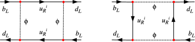
Figure 4: One-loop contributions $\Delta F=2$ amplitudes in the gaugeless limit.

An interesting aspect which is common to the electroweak loop functions in Eqs. (46) and (48) is the fact they diverge in the limit $m_{t}/m_{W}\to\infty$. This behavior is apparently strange: it contradicts the expectation that contributions of heavy particles at low energy decouple in the limit where their masses increase. The origin of this effect can be understand by noting that the leading contributions to both amplitudes are generated only by the Yukawa interaction. These contributions can be better isolated in the gaugeless limit of the SM, i.e. if we send to zero the gauge couplings. In this limit $m_{W}\to 0$ and the derivation of the effective Lagrangian discussed in Sect. 3.1 does not make sense. However, the leading contributions to the effective Lagrangians for $\Delta F=2$ and rare decays are unaffected. Indeed, the leading contributions to these processes are generated by Yukawa interactions of the type in Fig. 4, where the scalar fields are the Goldstone-bosons components of the Higgs field (which are not eaten up by the $W$ in the limit $g\to 0$). Since the top is still heavy, we can integrate it out, obtaining the following result for ${\cal L}_{\Delta B=2}$:

$$\left.{\cal L}^{\rm SM}_{\Delta B=2}\right|_{g_{i}\to 0}~{}=~{}\frac{G_{F}^{2}m_{t}^{2}}{16\pi^{2}}(V_{tb}^{*}V_{tq})^{2}(\bar{b}_{L}\gamma_{\mu}q_{L})^{2}~{}=~{}\frac{[(Y_{u}Y^{*}_{u})_{bq}]^{2}}{128\pi^{2}m_{t}^{2}}(\bar{b}_{L}\gamma_{\mu}q_{L})^{2}~{}.$$ (49)

Taking into account that $S_{0}(x)\to x/4$ for $x\to\infty$, it is easy to verify that this result is equivalent to the one in Eq. (48) in the large $m_{t}$ limit. A similar structure holds for the $\Delta F=1$ amplitude contributing to the axial operator $Q_{10A}$.

The last expression in Eq. (49), which holds in the limit where we neglect the charm Yukawa coupling, shows that the decoupling of the amplitude with the mass of the top is compensated by four powers of the top Yukawa coupling at the numerator. The divergence for $m_{t}\to\infty$ can thus be understood as the divergence of one of the fundamental couplings of the theory. Note also that in the gaugeless limit there is no GIM mechanism: the contributions of the various up-type quarks inside the loops do not cancel each other: they are directly weighted by the corresponding Yukawa couplings, and this is why the top-quark contribution is the dominant one.

This exercise illustrates the key role of the Yukawa coupling in determining the main properties flavour physics within the SM, as advertised in the first lecture. It also illustrates the interplay of flavour and electroweak symmetry breaking in determining the structure of short-distance dominated flavour-changing processes in the SM.

3.1.3 Hadronic matrix elements

As anticipated, all non-perturbative effects are confined in the hadronic matrix elements of the operators of the effective Lagrangians. As far as the evaluation of the matrix elements is concerned, we can divide $B$-physics observables in three main categories: i) inclusive decays, ii) one-hadron final states, iii) multi-hadron processes.

The heavy-quark expansion [15] form a solid theoretical framework to evaluate the hadronic matrix elements for inclusive processes: inclusive hadronic rates are related to those of free $b$ quarks, calculable in perturbation theory, by means of a systematic expansion in inverse powers of $\Lambda_{\rm QCD}/m_{b}$. Thanks to quark-hadron duality, the lowest-order terms in this expansion are the pure partonic rates, and for sufficiently inclusive observables higher-order corrections are usually very small. This technique has been very successful in the past in the case of charged-current semileptonic decays, as well as $B\to X_{s}\gamma$. However, it has a limited domain of applicability, due to the difficulty of selecting and reconstructing hadronic inclusive states. It cannot be used at hadronic machines, and even at $B$ factories it cannot be applied to very rare decays.

For processes with a single hadron in the final state, the hadronic effects are often (although not always) confined to the matrix elements of a single quark current. These can be expressed in terms of the meson decay constants

$$\langle 0|b\gamma_{\mu}\gamma_{5}q|B_{q}(p)\rangle=ip_{\mu}F_{B_{q}}~{},$$ (50)

or appropriate $B\to H$ hadronic form factors. Lattice QCD is the best tool to evaluate these non-perturbative quantities from first principles, at least in the kinematical region where the form factors are real (no re-scattering phase allowed). At present not all the form-factors relevant for $B$-physics phenomenology are computed on the lattice with good accuracy, but the field is evolving rapidly (see e.g. Ref. [16, 17]). To this category belong also the so-called bag-parameters for $\Delta B=2$ mixing, $B_{d,s}$, defined by

$$\eta_{B}(\mu)\langle\bar{B}_{q}|(\bar{b}_{L}\gamma_{\mu}q_{L})^{2}|B_{q}\rangle=\frac{2}{3}f_{B_{q}}^{2}m_{B_{q}}^{2}\eta_{B}(\mu)B_{q}(\mu)=\frac{2}{3}f_{B_{q}}^{2}m_{B_{q}}^{2}\hat{\eta}_{B}\hat{B}_{q}~{},$$ (51)

where both $\hat{B}_{q}$ and $\hat{\eta}_{B}$ are scale-independent quantities ($\hat{\eta}_{B}=0.55\pm 0.01$). For later convenience, we report here the lattice averages for meson decay constants and bag parameters obtained in Ref. [17]:

$$F_{B_{s}}=245\pm 25~{}{\rm GeV}~{},\qquad\quad\hat{B}_{s}=1.22\pm 0.12~{},$$ (52)

$$\frac{F_{B_{s}}}{F_{B_{d}}}=1.21\pm 0.04~{},\qquad\qquad\frac{\hat{B}_{B_{s}}}{\hat{B}_{B_{d}}}=1.00\pm 0.03~{}.$$ (53)

As can be seen, the absolute determinations are affected by ${\cal O}(10\%)$ errors, while the ratios, which are sensitive to $SU(3)$ breaking effects only, are known with a better precision. This is why the ratio $\Delta m_{B_{d}}/\Delta m_{B_{s}}$ gives more significant constraint in Fig. 1 rather than $\Delta m_{B_{d}}$ only.

The last class of hadronic matrix elements is the one of multi-hadron final states, such as the two-body non-leptonic decays $B\to\pi\pi$ and $B\to K\pi$, as well as many other processes with more than one hadron in the final state. These are the most difficult ones to be estimated from first principles with high accuracy. A lot of progress in the recent pass has been achieved thanks to QCD factorization [18] and the SCET [19] approaches, which provide factorization formulae to relate these hadronic matrix elements to two-body hadronic form factors in the large $m_{b}$ limit. However, it is fair to say that the errors associated to the $\Lambda_{\rm QCD}/m_{b}$ corrections are still quite large. This subject is quite interesting by itself, but is beyond the scope of these lectures, where we focus on clean $B$-physics observables for NP studies. To this purpose, the only interesting non-leptonic channels are those where, with suitable ratios, or using $SU(2)$ relations among hadronic matrix elements, we can eliminate completely all hadronic unknowns. Examples of this type are the $B\to DK$ channels discussed in Sect. 3.3.2.

3.2 Time evolution and of $B_{d,s}$ states

The non vanishing amplitude mixing a $B^{0}$ meson ($B^{0}_{d}$ or $B^{0}_{s}$) with the corresponding anti meson, described within the SM by the effective Lagrangian in Eq. 47, induces a time-dependent oscillations between $B^{0}$ and $\bar{B}^{0}$ states: an initially produced $B^{0}$ or $\bar{B}^{0}$ evolves in time into a superposition of $B^{0}$ and $\bar{B}^{0}$. Denoting by $\left|B^{0}(t)\right>$ (or $\left|\bar{B}^{0}(t)\right>$) the state vector of a $B$ meson which is tagged as a $B^{0}$ (or $\bar{B}^{0}$) at time $t=0$, the time evolution of these states is governed by the following equation:

$$i\frac{d}{dt}\left(\begin{array}[]{c}\left|B(t)\right>\\ \left|\bar{B}(t)\right>\end{array}\right)=\left(M-i\,\frac{\Gamma}{2}\right)\left(\begin{array}[]{c}\left|B(t)\right>\\ \left|\bar{B}(t)\right>\end{array}\right)~{},$$ (54)

where the mass-matrix $M$ and the decay-matrix $\Gamma$ are $t$-independent, Hermitian $2\times 2$ matrices. CPT invariance implies that $M_{11}=M_{22}$ and $\Gamma_{11}=\Gamma_{22}$, while the off-diagonal element $M_{12}=M_{21}^{*}$ is the one we can compute using the effective Lagrangian ${\cal L}_{\Delta B=2}$.

The mass eigenstates are the eigenvectors of $M-i\,\Gamma/2$. We express them in terms of the flavor eigenstates as

$$\left|B_{L}\right>=p\left|B^{0}\right>+q\left|\bar{B}^{0}\right>~{},\qquad\left|B_{H}\right>=p\left|B^{0}\right>-q\left|\bar{B}^{0}\right>~{},$$ (55)

with $|p|^{2}+|q|^{2}=1$. Note that, in general, $\left|B_{L}\right>$ and $\left|B_{H}\right>$ are not orthogonal to each other. The time evolution of the mass eigenstates is governed by the two eigenvalues $M_{H}-i\,\Gamma_{H}/2$ and $M_{L}-i\,\Gamma_{L}/2$:

$$\left|B_{H,L}(t)\right>=e^{-(iM_{H,L}+\Gamma_{H,L}/2)t}\,\left|B_{H,L}(t=0)\right>\,.$$ (56)

For later convenience it is also useful to define

$$m=\frac{M_{H}+M_{L}}{2},\qquad\Gamma=\frac{\Gamma_{L}+\Gamma_{H}}{2}~{},\qquad\Delta m=M_{H}-M_{L}~{},\qquad\Delta\Gamma=\Gamma_{L}-\Gamma_{H}~{}.$$ (57)

With these conventions the time evolution of initially tagged $B^{0}$ or $\bar{B}^{0}$ states is

$$\left|B^{0}(t)\right> = e^{-imt}\,e^{-\Gamma t/2}\left[f_{+}(t)\,\left|B^{0}\right>+\frac{q}{p}\,f_{-}(t)\,\left|\bar{B}^{0}\right>\right]~{},$$

$$\left|\bar{B}^{0}(t)\right> = e^{-imt}\,e^{-\Gamma t/2}\left[\frac{p}{q}\,f_{-}(t)\,\left|B^{0}\right>+f_{+}(t)\,\left|\bar{B}^{0}\right>~{}\right]~{},$$ (58)

where

$$f_{+}(t) = \phantom{-}\cosh\frac{\Delta\Gamma t}{4}\cos\frac{\Delta mt}{2}-i\sinh\frac{\Delta\Gamma t}{4}\sin\frac{\Delta mt}{2}~{},$$ (59)

$$f_{-}(t) = -\sinh\frac{\Delta\Gamma t}{4}\cos\frac{\Delta mt}{2}+i\cosh\frac{\Delta\Gamma t}{4}\sin\frac{\Delta mt}{2}~{},$$ (60)

In both $B_{s}$ and $B_{d}$ systems the following hierarchies holds: $|\Gamma_{12}|\ll|M_{12}|$ and $\Delta\Gamma\ll\Delta m$. They are experimentally verified and can be traced back to the fact that $|\Gamma_{12}|$ is a genuine long-distance ${\cal O}(G_{F}^{2})$ effect (it is indeed related to the absorptive part of the box diagrams in Fig. 3) which do not share the large $m_{t}$ enhancement of $|M_{12}|$ (which is a short-distance dominated quantity). Taking into account this hierarchy leads to the following approximate expressions for the quantities appearing in the time-evolution formulae in terms of $M_{12}$ and $\Gamma_{12}$:

$$\Delta m = 2\,|M_{12}|\left[1+{\cal O}\left(\left|\frac{\Gamma_{12}}{M_{12}}\right|^{2}\right)\right]~{},$$ (61)

$$\Delta\Gamma = 2\,|\Gamma_{12}|\cos\phi\left[1+{\cal O}\left(\left|\frac{\Gamma_{12}}{M_{12}}\right|^{2}\right)\right]~{},$$ (62)

$$\frac{q}{p} = -e^{-i\phi_{B}}\left[1-\frac{1}{2}\left|\frac{\Gamma_{12}}{M_{12}}\right|\sin\phi+{\cal O}\left(\left|\frac{\Gamma_{12}}{M_{12}}\right|^{2}\right)\right]~{},$$ (63)

where $\phi={\rm arg}(-M_{12}/\Gamma_{12})$ and $\phi_{B}$ is the phase of $M_{12}$. Note that $\phi_{B}$ thus defined is not measurable and depends on the phase convention adopted, while $\phi$ is a phase-convention quantity which can be measured in experiments.

Taking into account the above results, the time-dependent decay rates of an initially tagged $B^{0}$ or $\bar{B}^{0}$ state into some final state $f$ can be written as

$$\Gamma[B^{0}(t=0)\to f(t)]={\cal N}_{0}|A_{f}|^{2}e^{-\Gamma t}\Bigg{\{}\frac{1+|\lambda_{f}|^{2}}{2}\cosh\frac{\Delta\Gamma t}{2}$$

$$\qquad+\frac{1-|\lambda_{f}|^{2}}{2}\cos(\Delta mt)-{\rm Re}\,\lambda_{f}\sinh\frac{\Delta\Gamma t}{2}-{\rm Im}\,\lambda_{f}\sin(\Delta mt)\Bigg{\}},$$

$$\!\!\!\!\!\Gamma[\bar{B}^{0}(t=0)\to f(t)]={\cal N}_{0}|A_{f}|^{2}\left(1+\left|\frac{\Gamma_{12}}{M_{12}}\right|\sin\phi\right)e^{-\Gamma t}\Bigg{\{}\frac{1+|\lambda_{f}|^{2}}{2}\times$$

$$\times\cosh\frac{\Delta\Gamma t}{2}-\frac{1-|\lambda_{f}|^{2}}{2}\cos(\Delta mt)-{\rm Re}\,\lambda_{f}\sinh\frac{\Delta\Gamma t}{2}+{\rm Im}\,\lambda_{f}\sin(\Delta mt)\Bigg{\}}~{},$$

where ${\cal N}_{0}$ is the flux normalization and, following the standard notation, we have defined

$$\lambda_{f}=\frac{q}{p}\frac{\bar{A}_{f}}{A_{f}}\approx-e^{-i\phi_{B}}\,\frac{\bar{A}_{f}}{A_{f}}\left[1-\frac{1}{2}\left|\frac{\Gamma_{12}}{M_{12}}\right|\sin\phi\right]$$ (64)

in terms of the decay amplitudes

$$A_{f}=\langle f|{\cal L}_{\Delta F=1}\left|B^{0}\right>~{},\qquad\qquad\bar{A}_{f}=\langle f|{\cal L}_{\Delta F=1}\left|\bar{B}^{0}\right>~{}.$$ (65)

From the above expressions it is clear that the key quantity we can access experimentally in the time-dependent study of $B$ decays is the combination $\lambda_{f}$. Both real and imaginary parts of $\lambda_{f}$ can be measured, and indeed this is a phase-convention independent quantity: the phase convention in $\phi_{B}$ is compensated by the phase convention in the decay amplitudes. In other words, what we can measure is the weak-phase difference between $M_{12}$ and the decay amplitudes.

For generic final states, $\lambda_{f}$ is a quantity that is difficult to evaluate. However, it becomes particularly simple in the case where $f$ is a CP eigenstate, ${\rm CP}\left|f\right>=\eta_{f}\left|f\right>$, and the weak phase of the decaying amplitude is know. In such case $\bar{A}_{f}/A_{f}$ is a pure phase factor ($|\bar{A}_{f}/A_{f}|=1$), determined by the weak phase of the decaying amplitude:

$$\left.\lambda_{f}\right|_{\rm CP-eigen.}=\eta_{f}\frac{q}{p}e^{-2i\phi_{A}}~{},\qquad A_{f}=|A_{f}|e^{i\phi_{A}}~{},\qquad\eta_{f}=\pm 1~{}.$$ (66)

The most clean example of this type of channels is the $\left|\psi K_{S}\right>$ final state for $B_{d}$ decays. In this case the final state is a CP eigenstate and the decay amplitude is real (to a very good approximation) in the standard CKM phase convention. Indeed the underlying partonic transition is dominated by the Cabibbo-allowed tree-level process $b\to c\bar{c}s$, which has a vanishing phase in the standard CKM phase convention, and also the leading one-loop corrections (top-quark penguins) have the same vanishing weak phase. Since in the $B_{d}$ system we can safely neglect $\Gamma_{12}/M_{12}$, this implies

$$\lambda^{B_{b}}_{\psi K_{s}}=-e^{-i\phi_{B_{d}}}~{},\qquad{\rm Im}\,\left(\lambda^{B_{b}}_{\psi K_{s}}\right)_{\rm SM}=\sin(2\beta)~{},$$ (67)

where the SM expression of $\phi_{B_{d}}$ is nothing but the phase of the CKM combination $(V_{tb}^{*}V_{td})^{2}$ appearing in Eq. (47). Given the smallness of $\Delta\Gamma_{d}$, this quantity is easily extracted by the ratio

$$\frac{\Gamma[\bar{B}_{d}(t=0)\to\psi K_{s}(t)]-\Gamma[B^{0}(t=0)\to f\psi K_{s}(t)]}{\Gamma[\bar{B}_{d}(t=0)\to\psi K_{s}(t)]+\Gamma[B^{0}(t=0)\to f\psi K_{s}(t)]}\approx{\rm Im}\,\left(\lambda^{B_{b}}_{\psi K_{s}}\right)\sin(\Delta m_{B_{d}}t)~{},$$

which can be considered the golden measurement of $B$ factories.

Another class of interesting final states are CP-conjugate channels $\left|f\right>$ and $\left|\bar{f}\right>$ which are accessible only to $B^{0}$ or $\bar{B}^{0}$ states, such that $|A_{f}|=|\bar{A}_{\bar{f}}|$ and $\bar{A}_{f}=\bar{A}_{f}$=0. Typical examples of this type are the charged semileptonic channels. In this case the asymmetry

$$\frac{\Gamma[\bar{B}^{0}(t=0)\to f(t)]-\Gamma[B^{0}(t=0)\to\bar{f}(t)]}{\Gamma[\bar{B}^{0}(t=0)\to f(t)]+\Gamma[B^{0}(t=0)\to\bar{f}(t)]}=\left|\frac{\Gamma_{12}}{M_{12}}\right|\sin\phi\left[1+{\cal O}\left(\frac{\Gamma_{12}}{M_{12}}\right)\right]$$

turns out to be time-independent and a clean way to determine the indirect CP-violating phase $\phi$.

3.3 A selection of particularly interesting observables in the LHC era

Given the general arguments about the sensitivity to physics beyond the SM presented at the end of the first lecture, and the theoretical tool discussed above, in the following we analyse some interesting measurements which could be performed in the LHC era, and particularly at Tevatron and at the LHCb experiment. The list presented here is far from being exhaustive (for a more complete analysis we refer to the reviews in Ref. [5, 6, 7, 20]), but it should serve as an illustration of the interesting potential of $B$ physics at hadron colliders.

3.3.1 CP violation in $B_{s}$ mixing

The CP violating phase of $B_{s}$–$\bar{B}_{s}$ mixing is the last missing ingredient of down-type $\Delta F=2$ observables. The fact we have not found any deviations from the SM in $B_{d}$–$\bar{B}_{d}$ and $\Delta m_{B_{s}}$ should not discourage the measurement of this missing piece of the $\Delta F=2$ puzzle.

The golden channel for the measurement of the CP-violating phase of $B_{s}$–$\bar{B}_{s}$ mixing is the time-dependent analysis of the $B_{s}(\bar{B}_{s})\to\psi\phi$ decay. At the quark level $B_{s}\to\psi\phi$ share the same virtues of $B_{d}\to\psi K$ (partonic amplitude of the type $b\to c\bar{c}s$), which is used to extract the phase of $B_{d}$–$\bar{B}_{d}$ mixing. However, there a few points which makes this measurement much more challenging:

• The $B_{s}$ oscillations are much faster ($\Delta m_{B_{s}}/\Delta m_{B_{d}}\approx F^{2}_{B_{s}}/F^{2}_{B_{d}}|V_{ts}/V_{td}|^{2}$ $\approx 30$), making the time-dependent analysis quite difficult (and essentially inaccessible at $B$ factories).

• Contrary to $\left|\psi K\right>$, which has a single angular momentum and is a pure CP eigenstate, the vector-vector state $\left|\psi\phi\right>$ produced by the $B_{s}$ decay has different angular momenta, corresponding to different CP eigenstates. These must be disentangled with a proper angular analysis of the final four-body final state $\left|(\ell^{+}\ell^{-})_{\psi}(K^{+}K^{-})_{\phi}\right>$. To avoid contamination from the nearby $\left|\psi f_{0}\right>$ state, the fit should include also a $\left|(\ell^{+}\ell^{-})_{\psi}(K^{+}K^{-})_{S-{\rm wave}}\right>$ component, for a total of ten independent (and unknown) weak amplitudes.

• Contrary to the $B_{d}$ system, the width difference cannot be neglected in the $B_{s}$ case, leading to an additional key parameter to be included in the fit.

Modulo the experimental difficulties listed above, the process is theoretically clean and a complete fit of the decay distributions should allow the extraction of

$$\lambda^{B_{s}}_{\psi\phi}\approx-e^{-i\phi_{B_{s}}}~{},$$ (68)

where the SM prediction is

$$\phi_{B_{s}}^{\rm SM}=-{\rm arg}\frac{(V_{tb}^{*}V_{ts})^{2}}{|V_{tb}^{*}V_{ts}|^{2}}\approx-0.03~{}.$$ (69)

The tiny value of $\phi^{\rm SM}_{B_{s}}$ implies that, within the SM, no CP asymmetry should be observed in the near future. The present status of the combined fit of $\Delta\Gamma_{s}$ and $\phi_{B_{s}}$ from the CDF [22] and D0 [23] experiments at Tevatron is shown in Fig. 5. As can be noted, the agreement with the SM is not good, but the errors are still large.

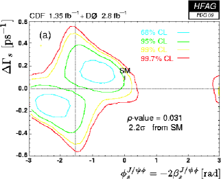
Figure 5: Combined fit of CDF and D0 results on $\Delta\Gamma$ and $\phi_{B_{s}}$ from the time-dependent analysis of $B_{s}\to\psi\phi$ decays, from Ref. [24].

As we will see in Sect. 4.1 a clear evidence for $\phi_{B_{s}}\not=0$ at Tevatron, or even within the first year of LHCb (which realistically would imply $|\phi_{B_{s}}|>0.1$), would not only signal the presence of physics beyond the SM, but would also rule out the whole class of MFV models.

3.3.2 CP violation in charged $B$ decays

Among non-leptonic channels $B^{\pm}\to DK$ decays are particularly interesting since, via appropriate asymmetries, allows us to extract the CKM angle $\gamma$ in a very clean way. The extraction of $\gamma$ involves only tree-level $B$ decay amplitudes, and is virtually free from hadronic uncertainties (which are eliminated directly by data). It is therefore an essential element for a precise determination of the SM Yukawa couplings also in presence of NP.

The main strategy is based on the following two observations:

• The partonic amplitudes for $B^{-}\to\bar{D}K^{-}$ ($b\to c\bar{u}s$) and $B^{-}\to\bar{D}K^{-}$ ($b\to u\bar{c}s$) are pure tree-level amplitudes (no penguins allowed given the four different quark flavours). As a result, their weak phase difference is completely determined and is $\gamma={\rm arg}\left(-V_{ud}V^{*}_{ub}/V_{cd}V^{*}_{cb}\right)$.

• Thanks to $D$–$\bar{D}$ mixing, there are several final states $f$ accessible to both $D$ and $\bar{D}$, where the two tree-level amplitudes can interfere. By combining the four final states $B^{\pm}\to fK^{\pm}$ and $B^{\pm}\to\bar{f}K^{\pm}$, we can extract $\gamma$ and all the relevant hadronic unknowns of the system.

The first strategy, proposed by Gronau, London, and Wyler [25] was based on the selection of $D(\bar{D})$ decays to two-body $CP$ eigenstates. But it has later been realized that any final state accessible to both $D$ and $\bar{D}$ (such as the $K^{\pm}\pi^{\mp}$ channels [26], or multibody final states [27]) may work as well.

Let’s start from the case of $D(\bar{D})$ decays to CP eigenstates, where the formalism is particularly transparent. The key quantity is the ratio

$$r_{B}e^{i\delta_{B}}=\frac{A(B^{+}\to D^{0}K^{+})}{A(B^{+}\to\bar{D}^{0}K^{+})}~{},$$ (70)

where $\delta$ is a strong phase. Denoting CP-even and CP-odd final states $f_{+}$ and $f_{-}$, we then have

$${A}\left(B^{-}\to f_{+}K^{-}\right) = A_{0}\times\left[1+r_{B}e^{i\left(\delta_{B}-\gamma\right)}\right]$$

$${A}\left(B^{-}\to f_{-}K^{-}\right) = A_{0}\times\left[1-r_{B}e^{i\left(\delta_{B}-\gamma\right)}\right]$$

$${A}\left(B^{+}\to f_{+}K^{+}\right) = A_{0}\times\left[1+r_{B}e^{i\left(\delta_{B}+\gamma\right)}\right]$$

$${A}\left(B^{+}\to f_{-}K^{+}\right) = A_{0}\times\left[1-r_{B}e^{i\left(\delta_{B}+\gamma\right)}\right]$$ (71)

It is clear that combining the four rates we can extract the three hadronic unknowns ($A_{0}$, $r_{B}$, and $\delta$) as well as $\gamma$. It is also clear that the sensitivity to $\gamma$ vanishes in the limit $r_{B}\to 0$, and indeed the main limitation of this method is that $r_{B}$ turns out to be very small.

The formalism is essentially unchanged if we consider final states that are not CP eigenstates, such as the $K^{\pm}\pi^{\mp}$ states. These have the advantage that the suppression of $r_{B}$ is partially compensated by the CKM suppression of the corresponding $D(\bar{D})\to K^{\pm}\pi^{\mp}$ decays. Indeed the effective relevant ratio becomes

$$r_{\rm eff}e^{i\delta_{\rm eff}}=\frac{A(B^{+}\to D^{0}K^{+})}{A(B^{+}\to\bar{D}^{0}K^{+})}~{},\times\frac{A(D^{0}\to K^{-}\pi^{+})}{A(\bar{D}^{0}\to K^{-}\pi^{+})}$$ (72)

which is substantially larger than $r_{B}$.

Once $r_{B}$ and $\delta_{B}$ (or $r_{\rm eff}$ and $\delta_{\rm eff}$) are determined from data, the extraction of $\gamma$ has essentially no theoretical uncertainty. In principle a theoretical error could be induced by the neglected CP-violating effects in charm mixing. In practice, the experimental bounds on charm mixing make this effect totally negligible. The key issue is only collecting high statistics on this highly-suppressed decay modes: a clear target for $B$ physics at hadron machines.

3.3.3 The forward-backward asymmetry in $B\to K^{*}\ell^{+}\ell^{-}$.

Theoretical predictions for exclusive FCNC decays are not easy. Even if the final state involve only one hadron, in most of the kinematical region re-scattering effects of the type $B\to K^{*}H\bar{H}\to K^{*}\ell^{+}\ell^{-}$ are possible, making difficult to estimate precisely the decay rate. However, the largest source of uncertainty is typically the normalization of the hadronic form factors. The theoretical error can be substantially reduced in appropriate ratios or differential distributions. A clean example of this type is the normalized forward-backward asymmetry in $B\to K^{*}\ell^{+}\ell^{-}$.

The observable is defined as

$${\cal A}_{FB}(s)=\frac{1}{d\Gamma(B\to K^{*}\mu^{+}\mu^{-})/ds}\int_{-1}^{1}d\cos\theta~{}\frac{d^{2}\Gamma(B\to K^{*}\mu^{+}\mu^{-})}{ds~{}d\cos\theta}\mbox{sgn}(\cos\theta)~{},$$ (73)

where $\theta$ is the angle between the momenta of $\mu^{+}$ and $\bar{B}$ in the dilepton center-of-mass frame. Assuming that the leptonic current has only a vector ($V$) or axial-vector ($A$) structure (as in the SM), the FB asymmetry provides a direct measure of the $A$–$V$ interference. Indeed, at the lowest-order one can write

$${\cal A}_{\rm FB}(q^{2})\propto{\rm Re}\left\{C_{10A}^{*}\left[\frac{q^{2}}{m_{b}^{2}}C_{9V}^{\rm eff}+r(q^{2})\frac{m_{b}C_{7\gamma}}{m_{B}}\right]\right\}~{},$$

where $r(q^{2})$ is an appropriate ratio of $B\to K^{*}$ vector and tensor form factors [28]. There are three main features of this observable that provide a clear and independent short-distance information:

1. The position of the zero ($q_{0}$) of ${\cal A}_{\rm FB}(q^{2})$ in the low-$q^{2}$ region (see Fig. 6) [28]: as shown by means of a full NLO calculation [29], the experimental measurement of $q^{2}_{0}$ could allow a determination of $C_{7}/C_{9}$ at the $10\%$ level.

2. The sign of ${\cal A}_{\rm FB}(q^{2})$ around the zero. This is fixed unambiguously in terms of the relative sign of $C_{10}$ and $C_{9}$: within the SM one expects ${\cal A}_{\rm FB}(q^{2}>q^{2}_{0})>0$ for $|\bar{B}\rangle\equiv|b\bar{d}\rangle$ mesons.

3. The relation ${\cal A}[\bar{B}]_{\rm FB}(q^{2})=-{\cal A}[B]_{\rm FB}(q^{2})$. This follows from the CP-odd structure of ${\cal A}_{\rm FB}$ and holds at the $10^{-3}$ level within the SM [30], where $C_{10}$ has a negligible CP-violating phase.

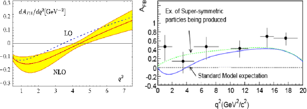
Figure 6: Left: SM prediction for the zero of the forward-backward asymmetry in $B^{-}\to K^{*-}\ell^{+}\ell^{-}$ at LO and NLO (the band indicates the theoretical uncertainty) [29]. Right: Recent measurement of the forward-backward asymmetry in $B^{-}\to K^{*-}\ell^{+}\ell^{-}$ by BELLE [31]

The present status of the measurement at BELLE [31] is shown in Fig. 6. Also in this case, similarly to $B_{s}$–$\bar{B}_{s}$ mixing, the agreement with the SM is not good, leaving open the room for speculations about sizable non-standard effects. However, the errors are clearly too large to draw definite conclusions.

3.3.4 $B\to\ell^{+}\ell^{-}$

The purely leptonic decays constitute a special case among exclusive transitions. Within the SM only the axial-current operator, $Q_{10A}$, induces a non-vanishing contribution to these decays. As a result, the short-distance contribution is not diluted by the mixing with four-quark operators. Moreover, the hadronic matrix element involved is the simplest we can consider, namely the $B$-meson decay constant in Eq. (50). As we have seen, present estimates of $F_{B_{d}}$ and $F_{B_{s}}$ from lattice QCD are already at the $10\%$ level, and in the future the error is expected to go below $5\%$.

The price to pay for this theoretically-clean amplitude is a strong helicity suppression for $\ell=\mu$ (and $\ell=e$), or the channels with the best experimental signature. Employing the full NLO expression of $C^{\rm SM}_{10A}$, we can write [32]

$${\mathcal{B}}(B_{s}\to\mu^{+}\mu^{-})^{\rm SM}=3.1\times 10^{-9}\left(\frac{|V_{ts}|}{0.04}\right)^{2}\times\left(\frac{F_{B_{s}}}{0.21~{}\mbox{GeV}}\right)^{2}\!\!$$ (74)

$$\frac{{\mathcal{B}}(B_{s}\to\tau^{+}\tau^{-})^{\rm SM}}{{\mathcal{B}}(B_{s}\to\mu^{+}\mu^{-})^{\rm SM}}=215~{},\qquad\frac{{\mathcal{B}}(B_{s}\to e^{+}e^{-})^{\rm SM}}{{\mathcal{B}}(B_{s}\to\mu^{+}\mu^{-})^{\rm SM}}=2.4\times 10^{-5}~{}.$$ (75)

The corresponding $B_{d}$ modes are both suppressed by an additional factor $|V_{td}/V_{ts}|^{2}F^{2}_{B_{d}}/F^{2}_{B_{s}}\approx 1/30$. The present experimental bound closest to SM expectations is the one obtained by CDF on $B_{s}\to\mu^{+}\mu^{-}$ [33]

$${\mathcal{B}}(B_{s}\to\mu^{+}\mu^{-})<5.8\times 10^{-8}\quad(95\%\;\;{\rm CL})~{},$$ (76)

which is about one order of magnitude above the SM level.

The strong helicity suppression and the theoretical cleanness make these modes excellent probes of several new-physics models and, particularly, of scalar FCNC amplitudes. Scalar FCNC operators, such as $\bar{b}_{R}s_{L}\bar{\mu}_{R}\mu_{L}$, are present within the SM but are negligible because of the smallness of down-type Yukawa couplings. On the other hand, these amplitudes could be non-negligible in models with an extended Higgs sector (see Sect. 4.1.2). In particular, within the MSSM, where two Higgs doublets are coupled separately to up- and down-type quarks, a strong enhancement of scalar FCNCs can occur at large $\tan\beta=v_{u}/v_{d}$. This effect is very small in non-helicity-suppressed $B$ decays (because of the small Yukawa couplings), but could easily enhance $B\to\ell^{+}\ell^{-}$ rates by one order of magnitude.

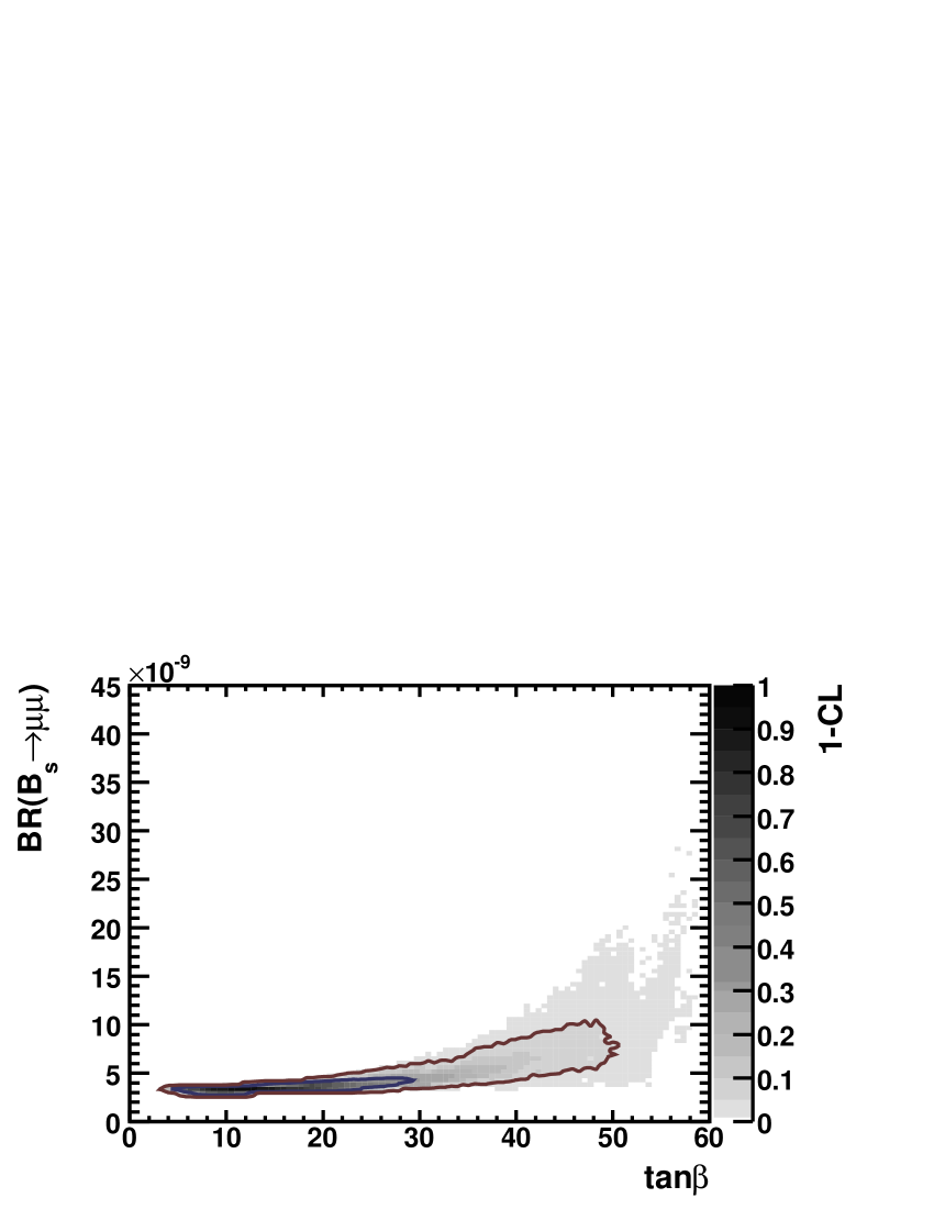
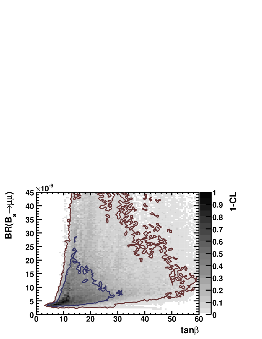
Figure 7: The correlation between branching ratio for $B_{s}\to\mu^{+}\mu^{-}$ and $\tan\beta$ in the CMSSM (left panel) and in the CMSSM with non-universal Higgs masses (right panel, see Sect. 4.2.2 for more details), from Ref. [34].

An illustration of the possible enhancement in a constrained version of the MSSM (that will be discussed in Sect. 4.2.2) is shown in Fig. 7. This figure shows that the present search for $B_{s}\to\mu^{+}\mu^{-}$ at CDF is already quite interesting, even if the sensitivity is well above the SM level. In a long-term perspective, the discovery and precise measurement of all the accessible $B\to\ell^{+}\ell^{-}$ channels is definitely one of the most interesting items of the $B$-physics program at hadron colliders.

4 Flavour physics beyond the SM: models and predictions

4.1 Minimal Flavour Violation

The main idea of MFV is that flavour-violating interactions are linked to the known structure of Yukawa couplings also beyond the SM. In a more quantitative way, the MFV construction consists in identifying the flavour symmetry and symmetry-breaking structure of the SM and enforce it also beyond the SM.

The MFV hypothesis consists of two ingredients [35]: (1) a flavor symmetry and (ii) a set of symmetry-breaking terms. The symmetry is noting but the large global symmetry ${\mathcal{G}}_{\rm flavour}$ of the SM Lagrangian in absence of Yukawa couplings shown in Eq. (4). Since this global symmetry, and particularly the ${SU}(3)$ subgroups controlling quark flavor-changing transitions, is already broken within the SM, we cannot promote it to be an exact symmetry of the NP model. Some breaking would appear at the quantum level because of the SM Yukawa interactions. The most restrictive assumption we can make to protect in a consistent way quark-flavor mixing beyond the SM is to assume that $Y_{d}$ and $Y_{u}$ are the only sources of flavour symmetry breaking also in the NP model. To implement and interpret this hypothesis in a consistent way, we can assume that ${\mathcal{G}}_{q}$ is a good symmetry and promote $Y_{u,d}$ to be non-dynamical fields (spurions) with non-trivial transformation properties under ${\mathcal{G}}_{q}$:

$$Y_{u}\sim(3,\bar{3},1)~{},\qquad Y_{d}\sim(3,1,\bar{3})~{}.\qquad$$ (77)

If the breaking of the symmetry occurs at very high energy scales, at low-energies we would only be sensitive to the background values of the $Y$, i.e. to the ordinary SM Yukawa couplings. The role of the Yukawa in breaking the flavour symmetry becomes similar to the role of the Higgs in the the breaking of the gauge symmetry. However, in the case of the Yukawa we don’t know (and we do not attempt to construct) a dynamical model which give rise to this symmetry breaking.

Within the effective-theory approach to physics beyond the SM introduced in Sect. 2.4, we can say that an effective theory satisfies the criterion of Minimal Flavor Violation in the quark sector if all higher-dimensional operators, constructed from SM and $Y$ fields, are invariant under CP and (formally) under the flavor group ${\mathcal{G}}_{q}$ [35].

According to this criterion one should in principle consider operators with arbitrary powers of the (dimensionless) Yukawa fields. However, a strong simplification arises by the observation that all the eigenvalues of the Yukawa matrices are small, but for the top one, and that the off-diagonal elements of the CKM matrix are very suppressed. Working in the basis in Eq. (6) we have

$$\left[Y_{u}(Y_{u})^{\dagger}\right]^{n}_{i\not=j}~{}\approx~{}y_{t}^{n}V^{*}_{it}V_{tj}~{}.$$ (78)

As a consequence, in the limit where we neglect light quark masses, the leading $\Delta F=2$ and $\Delta F=1$ FCNC amplitudes get exactly the same CKM suppression as in the SM:

$$\mathcal{A}(d^{i}\to d^{j})_{\rm MFV} = (V^{*}_{ti}V_{tj})^{\phantom{a}}\mathcal{A}^{(\Delta F=1)}_{\rm SM}\left[1+a_{1}\frac{16\pi^{2}M^{2}_{W}}{\Lambda^{2}}\right]~{},$$ (79)

$$\mathcal{A}(M_{ij}-\bar{M}_{ij})_{\rm MFV} = (V^{*}_{ti}V_{tj})^{2}\mathcal{A}^{(\Delta F=2)}_{\rm SM}\left[1+a_{2}\frac{16\pi^{2}M^{2}_{W}}{\Lambda^{2}}\right]~{}.$$ (80)

where the $\mathcal{A}^{(i)}_{\rm SM}$ are the SM loop amplitudes and the $a_{i}$ are $\mathcal{O}(1)$ real parameters. The $a_{i}$ depend on the specific operator considered but are flavor independent. This implies the same relative correction in $s\to d$, $b\to d$, and $b\to s$ transitions of the same type: a key prediction which can be tested in experiment.

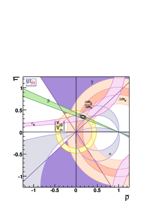
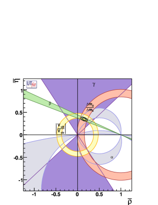
Figure 8: Fit of the CKM unitarity triangle (in 2008) within the SM (left) and in generic extensions of the SM satisfying the MFV hypothesis (right) [12].

As pointed out in Ref. [36], within the MFV framework several of the constraints used to determine the CKM matrix (and in particular the unitarity triangle) are not affected by NP. In this framework, NP effects are negligible not only in tree-level processes but also in a few clean observables sensitive to loop effects, such as the time-dependent CPV asymmetry in $B_{d}\to\psi K_{L,S}$. Indeed the structure of the basic flavor-changing coupling in Eq. (80) implies that the weak CPV phase of $B_{d}$–$\bar{B}_{d}$ mixing is arg[$(V_{td}V_{tb}^{*})^{2}$], exactly as in the SM. This construction provides a natural (a posteriori) justification of why no NP effects have been observed in the quark sector: by construction, most of the clean observables measured at $B$ factories are insensitive to NP effects in the MFV framework. A comparison of the CKM fits in the SM and in generic MFV models is shown in Fig. 8. Essentially only $\epsilon_{K}$ and $\Delta m_{B_{d}}$ (but not the ratio $\Delta m_{B_{d}}/\Delta m_{B_{s}}$) are sensitive to non-standard effects within MFV models.

Given the built-in CKM suppression, the bounds on higher-dimensional operators in the MFV framework turns out to be in the TeV range. This can easily be understood by the discussion in Sect. 2.4.1: the MFV bounds on operators contributing to $\epsilon_{K}$ and $\Delta m_{B_{d}}$ are obtained from Eq. (32) setting $|c_{ij}|=|y_{t}^{2}V_{3i}^{*}V_{3j}|^{2}$. From this perspective we could say that the MFV hypothesis provides a solution to the flavour problem.

4.1.1 General considerations

The idea that the CKM matrix rules the strength of FCNC transitions also beyond the SM is a concept that has been implemented and discussed in several works, especially after the first results of the $B$ factories (see e.g. Ref. [37, 38]). However, it is worth stressing that the CKM matrix represents only one part of the problem: a key role in determining the structure of FCNCs is also played by quark masses, or better by the Yukawa eigenvalues. In this respect, the above MFV criterion provides the maximal protection of FCNCs (or the minimal violation of flavour symmetry), since the full structure of Yukawa matrices is preserved. Moreover, contrary to other approaches, the above MFV criterion is based on a renormalization-group-invariant symmetry argument, which can easily be extended to TeV-scale effective theories where new degrees of freedoms, such as extra Higgs doublets or SUSY partners of the SM fields are included.

In particular, it is worth stressing that the MFV hypothesis can be implemented also in the so-called Higgsless models, i.e. assuming that the breaking of the electroweak symmetry is induced by some strong dynamics at the TeV scale (similarly tot he breaking of chiral symmetry in QCD). In this case Eq. (3) is replaced by an effective interaction between fermion fields and the Goldstone bosons associated to the spontaneous breaking of the gauge symmetry. From the point of view of the flavour symmetry, this interaction is identical to the one in (3), and this allows us to proceed as in the case with the explicit Higgs field (see e.g. Ref. [39]). The only difference between weakly- and strongly-interacting theories at the TeV scale is that in the latter case the expansion in powers of the Yukawa spurions is not necessarily a rapidly convergent series. If this is the case, then a resummation of the terms involving the top-quark Yukawa coupling needs to be performed [40]

This model-independent structure does not hold in most of the alternative definitions of MFV models that can be found in the literature. For instance, the definition of Ref. [38] (denoted constrained MFV, or CMFV) contains the additional requirement that the effective FCNC operators playing a significant role within the SM are the only relevant ones also beyond the SM. This condition is realized only in weakly coupled theories at the TeV scale with only one light Higgs doublet, such as the MSSM with small $\tan\beta$. It does not hold in several other frameworks, such as Higgsless models, or the MSSM with large $\tan\beta$.

Although the MFV seems to be a natural solution to the flavor problem, it should be stressed that we are still very far from having proved the validity of this hypothesis from data. A proof of the MFV hypothesis can be achieved only with a positive evidence of physics beyond the SM exhibiting the flavor-universality pattern (same relative correction in $s\to d$, $b\to d$, and $b\to s$ transitions of the same type) predicted by the MFV assumption. While this goal is quite difficult to be achieved, the MFV framework is quite predictive and thus could easily be falsified. Some of the most interesting predictions which could be tested in the near future are the following:

• No new CPV phases in $B_{s}$ mixing, hence $|\phi_{B_{s}}|<0.05$ from ${\cal A}_{\rm CP}(B_{s}\to\psi\phi)$.

• Ratio of $B_{s}$ and $B_{d}$ decays into $\ell^{+}\ell^{-}$ pairs determined by the CKM matrix: ${\cal B}(B_{d}\to\ell^{+}\ell^{-})/{\cal B}(B_{s}\to\ell^{+}\ell^{-})\approx|V_{td}/V_{ts}|^{2}$.

• No new CPV phases in $b\to s\gamma$, hence vanishingly small CP asymmetries in $B\to K^{*}\gamma$ and $B\to K^{*}\ell^{+}\ell^{-}$.

Violations of these bounds would not only imply physics beyond the SM, but also a clear signal of new sources of flavour symmetry breaking beyond the Yukawa couplings.

4.1.2 MFV at large $\tan\beta$.

If the Yukawa Lagrangian contains more than one Higgs field, we can still assume that the Yukawa couplings are the only irreducible breaking sources of ${\mathcal{G}}_{q}$, but we can change their overall normalization. A particularly interesting scenario is the two-Higgs-doublet model where the two Higgses are coupled separately to up- and down-type quarks:

$$\mathcal{L}^{2HDM}_{Y}={\bar{Q}}_{L}\lambda_{d}D_{R}\phi_{D}+{\bar{Q}}_{L}Y_{u}U_{R}\phi_{U}+{\bar{L}}_{L}Y_{e}E_{R}\phi_{D}{\rm~{}+~{}h.c.}$$ (81)

This Lagrangian is invariant under an extra ${U}(1)$ symmetry with respect to the one-Higgs Lagrangian in Eq. (3): a symmetry under which the only charged fields are $D_{R}$ and $E_{R}$ (charge $+1$) and $\phi_{D}$ (charge $-1$). This symmetry, denoted ${U}_{\rm PQ}$, prevents tree-level FCNCs and implies that $Y_{u,d}$ are the only sources of ${\mathcal{G}}_{q}$ breaking appearing in the Yukawa interaction (similar to the one-Higgs-doublet scenario). Coherently with the MFV hypothesis, we can then assume that $Y_{u,d}$ are the only relevant sources of ${\mathcal{G}}_{q}$ breaking appearing in all the low-energy effective operators. This is sufficient to ensure that flavour-mixing is still governed by the CKM matrix, and naturally guarantees a good agreement with present data in the $\Delta F=2$ sector. However, the extra symmetry of the Yukawa interaction allows us to change the overall normalization of $Y_{u,d}$ with interesting phenomenological consequences in specific rare modes.

The normalization of the Yukawa couplings is controlled by the ratio of the vacuum expectation values of the two Higgs fields, or by the parameter $\tan\beta=\langle\phi_{U}\rangle/\langle\phi_{D}\rangle=v_{u}/v_{d}$. Defining the eigenvalues $\lambda_{u,d}$ as in Eq. (6),

$$\lambda_{u} = \frac{1}{v_{u}}{\rm diag}(m_{u},m_{c},m_{t})~{},$$

$$\lambda_{d} = \frac{1}{v_{d}}{\rm diag}(m_{d},m_{s},m_{b})=\frac{\tan\beta}{v_{u}}{\rm diag}(m_{d},m_{s},m_{b}).$$ (82)

For $\tan\beta>\!\!>1$ the smallness of the $b$ quark can be attributed to the smallness of of $v_{d}$ with respect to $v_{u}\approx v$, rather than to the smallness of the corresponding Yukawa coupling. As a result, for $\tan\beta>\!\!>1$ we cannot anymore neglect down-type Yukawa couplings. Since the $b$-quark Yukawa coupling becomes $\mathcal{O}(1)$, the large-$\tan\beta$ regime is particularly interesting for all the helicity-suppressed observables in $B$ physics (i.e. the observables suppressed within the SM by the smallness of the $b$-quark Yukawa coupling).

Another important aspect of this scenario is that the the ${U}(1)_{\rm PQ}$ symmetry cannot be exact: it has to be broken at least in the scalar potential in order to avoid the presence of a massless pseudoscalar Higgs boson. Even if the breaking of ${U}(1)_{\rm PQ}$ and ${\mathcal{G}}_{q}$ are decoupled, the presence of ${U}(1)_{\rm PQ}$ breaking sources can have important implications on the structure of the Yukawa interaction, especially if $\tan\beta$ is large [42, 43]. We can indeed consider new dimension-four operators such as

$$\epsilon~{}{\bar{Q}}_{L}\lambda_{d}D_{R}\tilde{\phi}_{U}\qquad{\rm or}\qquad\epsilon~{}{\bar{Q}}_{L}\lambda_{u}\lambda_{u}^{\dagger}\lambda_{d}D_{R}\tilde{\phi}_{U}~{},$$ (83)

where $\epsilon$ denotes a generic MFV-invariant ${U}(1)_{\rm PQ}$-breaking source. Even if $\epsilon\ll 1$, the product $\epsilon\times\tan\beta$ can be $\mathcal{O}(1)$, inducing large corrections to the down-type Yukawa sector:

$$\epsilon~{}{\bar{Q}}_{L}\lambda_{d}D_{R}\tilde{\phi}_{U}\ \stackrel{{\scriptstyle vev}}{{\longrightarrow}}\ \epsilon~{}{\bar{Q}}_{L}\lambda_{d}D_{R}\langle\phi_{U}\rangle=(\epsilon\times\tan\beta)~{}{\bar{Q}}_{L}\lambda_{d}D_{R}\langle\phi_{D}\rangle~{}.$$ (84)

This is what happens in supersymmetry, where the operators in Eq. (83) are generated at the one-loop level [$\epsilon\sim 1/(16\pi^{2})$], and the large $\tan\beta$ solution is particularly welcome in the contest of Grand Unified models [44].

One of the clearest phenomenological consequences is a suppression (typically in the $10-50\%$ range) of the $B\to\ell\nu$ decay rate with respect to its SM expectation [45]. But the most striking signature could arise from the rare decays $B_{s,d}\to\ell^{+}\ell^{-}$ whose rates could be enhanced over the SM expectations by more than one order of magnitude [46] as already shown in Fig. 7 in the context of supersymmetric models. An enhancement of both $B_{s}\to\ell^{+}\ell^{-}$ and $B_{d}\to\ell^{+}\ell^{-}$ respecting the MFV relation $\Gamma(B_{s}\to\ell^{+}\ell^{-})/\Gamma(B_{d}\to\ell^{+}\ell^{-})\approx F^{2}_{B_{s}}/F^{2}_{B_{d}}|V_{ts}/V_{td}|^{2}$ would be an unambiguous signature of MFV at large $\tan\beta$ [47, 41].

4.2 Flavour breaking in the MSSM

The Minimal Supersymmetric extension of the SM (MSSM) is one of the most well-motivated and definitely the most studied extension of the SM at the TeV scale. For a detailed discussion of this model we refer to the review in Ref. [48] and to the lectures by J. Ellis at this school. Here we limit our self to analyse some properties of this model relevant to flavor physics.

The particle content of the MSSM consists of the SM gauge and fermion fields plus a scalar partner for each quark and lepton (squarks and sleptons) and a spin-1/2 partner for each gauge field (gauginos). The Higgs sector has two Higgs doublets with the corresponding spin-1/2 partners (higgsinos) and a Yukawa coupling of the type in Eq. (81). While gauge and Yukawa interactions of the model are completely specified in terms of the corresponding SM couplings, the so-called soft-breaking sector of the theory contains several new free parameters, most of which are related to flavor-violating observables. For instance the $6\times 6$ mass matrix of the up-type squarks, after the up-type Higgs field gets a vev ($\phi_{U}\to\langle\phi_{U}\rangle$), has the following structure

$${\tilde{M}}_{U}^{2}=\left(\begin{array}[]{cc}{\tilde{m}}_{Q_{L}}^{2}&A_{U}\langle\phi_{U}\rangle\\ A_{U}^{\dagger}\langle\phi_{U}\rangle&{\tilde{m}}_{U_{R}}^{2}\end{array}\right)~{}+~{}\mathcal{O}\left(m_{Z},m_{\rm top}\right)~{},$$ (85)

where ${\tilde{m}}_{Q_{L}}$, ${\tilde{m}}_{U_{R}}$, and $A_{U}$ are $3\times 3$ unknown matrices. Indeed the adjective minimal in the MSSM acronyms refers to the particle content of the model but does not specify its flavor structure.

Because of this large number of free parameters, we cannot discuss the implications of the MSSM in flavor physics without specifying in more detail the flavor structure of the model. The versions of the MSSM analyzed in the literature range from the so-called Constrained MSSM (CMSSM), where the complete model is specified in terms of only four free parameters (in addition to the SM couplings), to the MSSM without $R$ parity and generic flavor structure, which contains a few hundreds of new free parameters.

Throughout the large amount of work in the past decades it has became clear that the MSSM with generic flavor structure and squarks in the TeV range is not compatible with precision tests in flavor physics. This is true even if we impose $R$ parity, the discrete symmetry which forbids single s-particle production, usually advocated to prevent a too fast proton decay. In this case we have no tree-level FCNC amplitudes, but the loop-induced contributions are still too large compared to the SM ones unless the squarks are highly degenerate or have very small intra-generation mixing angles. This is nothing but a manifestation in the MSSM context of the general flavor problem illustrated in the first lecture.

The flavor problem of the MSSM is an important clue about the underling mechanism of supersymmetry breaking. On general grounds, mechanisms of SUSY breaking with flavor universality (such as gauge mediation) or with heavy squarks (especially in the case of the first two generations) tends to be favored. However, several options are still open. These range from the very restrictive CMSSM case, which is a special case of MSSM with MFV, to more general scenarios with new small but non-negligible sources of flavor symmetry breaking.

4.2.1 Flavor Universality, MFV, and RGE in the MSSM.

Since the squark fields have well-defined transformation properties under the SM quark-flavor group ${\mathcal{G}}_{q}$, the MFV hypothesis can easily be implemented in the MSSM framework following the general rules outlined in Sect. 4.1.

We need to consider all possible interactions compatible with i) softly-broken supersymmetry; ii) the breaking of ${\mathcal{G}}_{q}$ via the spurion fields $Y_{U,D}$. This allows to express the squark mass terms and the trilinear quark-squark-Higgs couplings as follows [49, 35]:

$${\tilde{m}}_{Q_{L}}^{2} = {\tilde{m}}^{2}\left(a_{1}{1{\rm l}}+b_{1}Y_{U}Y_{U}^{\dagger}+b_{2}Y_{D}Y_{D}^{\dagger}+b_{3}Y_{D}Y_{D}^{\dagger}Y_{U}Y_{U}^{\dagger}+\ldots\right)~{},$$

$${\tilde{m}}_{U_{R}}^{2} = {\tilde{m}}^{2}\left(a_{2}{1{\rm l}}+b_{5}Y_{U}^{\dagger}Y_{U}+\ldots\right)~{},\qquad$$

$$A_{U} = ~{}A\left(a_{3}{1{\rm l}}+b_{6}Y_{D}Y_{D}^{\dagger}+\ldots\right)Y_{U}~{},\qquad$$ (86)

and similarly for the down-type terms. The dimensional parameters $\tilde{m}$ and $A$, expected to be in the range few 100 GeV – 1 TeV, set the overall scale of the soft-breaking terms. In Eq. (86) we have explicitly shown all independent flavor structures which cannot be absorbed into a redefinition of the leading terms (up to tiny contributions quadratic in the Yukawas of the first two families), when $\tan\beta$ is not too large and the bottom Yukawa coupling is small, the terms quadratic in $Y_{D}$ can be dropped.

In a bottom-up approach, the dimensionless coefficients $a_{i}$ and $b_{i}$ should be considered as free parameters of the model. Note that this structure is renormalization-group invariant: the values of $a_{i}$ and $b_{i}$ change according to the Renormalization Group (RG) flow, but the general structure of Eq. (86) is unchanged. This is not the case if the $b_{i}$ are set to zero, corresponding to the so-called hypothesis of flavor universality. In several explicit mechanism of supersymmetry breaking, the condition of flavor universality holds at some high scale $M$, such as the scale of Grand Unification in the CMSSM (see below) or the mass-scale of the messenger particles in gauge mediation (see Ref. [50]). In this case non-vanishing $b_{i}\sim(1/4\pi)^{2}\ln M^{2}/{\tilde{M}}^{2}$ are generated by the RG evolution. As recently pointed out in Ref. [51] the RG flow in the MSSM-MFV framework exhibit quasi infra-red fixed points: even if we start with all the $b_{i}=\mathcal{O}(1)$ at some high scale, the only non-negligible terms at the TeV scale are those associated to the $Y_{U}Y_{U}^{\dagger}$ structures.

If we are interested only in low-energy processes we can integrate out the supersymmetric particles at one loop and project this theory into the general MFV effective theory approach discussed before. In this case the coefficients of the dimension-six effective operators written in terms of SM and Higgs fields are computable in terms of the supersymmetric soft-breaking parameters. The typical effective scale suppressing these operators (assuming an overall coefficient $1/\Lambda^{2}$) is $\Lambda\sim 4\pi\tilde{m}$. Since the bounds on $\Lambda$ within MFV are in the few TeV range, we then conclude that if MFV holds, the present bounds on FCNCs do not exclude squarks in the few hundred GeV mass range, i.e. well within the LHC reach.

4.2.2 The CMSSM framework.

The CMSSM, also known as mSUGRA, is the supersymmetric extension of the SM with the minimal particle content and the maximal number of universality conditions on the soft-breaking terms. At the scale of Grand Unification ($M_{\rm GUT}\sim 10^{16}$ GeV) it is assumed that there are only three independent soft-breaking terms: the universal gaugino mass (${\tilde{m}}_{1/2}$), the universal trilinear term ($A$), and the universal sfermion mass ($\tilde{m}_{0}$). The model has two additional free parameters in the Higgs sector (the so-called $\mu$ and $B$ terms), which control the vacuum expectation values of the two Higgs fields (determined also by the RG running from the unification scale down to the electroweak scale). Imposing the correct $W$- and $Z$-boson masses allow us to eliminate one of these Higgs-sector parameters, the remaining one is usually chosen to be $\tan\beta$. As a result, the model is fully specified in terms of the three high-energy parameters $\{{\tilde{m}}_{1/2},{\tilde{m}}_{0},A\}$, and the low-energy parameter $\tan\beta$. This constrained version of the MSSM is an example of a SUSY model with MFV. Note, however, that the model is much more constrained than the general MSSM with MFV: in addition to be flavor universal, the soft-breaking terms at the unification scale obey various additional constraints (e.g. in Eq. (86) we have $a_{1}=a_{2}$ and $b_{i}=0$).

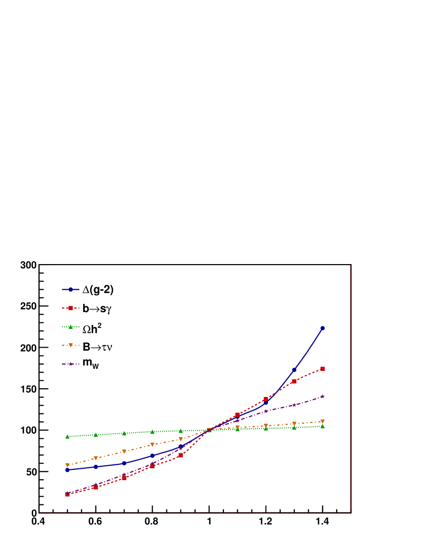
Figure 9: Relative sizes of the 95% C.L. preferred area in the $(m_{0},\tan\beta)$ plane of the CMSSM, as a function hypothetical variations of the present errors on $(g-2)_{\mu}$, the cold dark-matter abundance ($\Omega h^{2}$), ${\cal B}(B\to X_{s}\gamma)$, ${\cal B}(B^{+}\to\tau^{+}\nu)$, and $m_{W}$ [52]. The error scaling is relative to the current combined theory and experimental error.

In the MSSM with $R$ parity we can distinguish five main classes of one-loop diagrams contributing to FCNC and CP violating processes with external down-type quarks. They are distinguished according to the virtual particles running inside the loops: $W$ and up-quarks (i.e. the leading SM amplitudes), charged-Higgs and up-quarks, charginos and up-squarks, neutralinos and down-squarks, gluinos and down-squarks. Within the CMSSM, the charged-Higgs and chargino exchanges yield the dominant non-standard contributions.

Given the low number of free parameters, the CMSSM is very predictive and phenomenologically constrained by the precision measurements in flavor physics. The most powerful low-energy constraint comes from $B\to X_{s}\gamma$. For large values of $\tan\beta$, strong constraints are also obtained from $B_{s}\to\mu^{+}\mu^{-}$, and $B^{+}\to\tau^{+}\nu$. If these observables are within the present experimental bounds, the constrained nature of the model implies essentially no observable deviations from the SM in other flavor-changing processes. Interestingly enough, the CMSSM satisfy at the same time the flavor constraints and those from electroweak precision observables for squark masses below 1 TeV [52]. An illustration of the constraining power of the flavour observables in determining the allowed parameter space of the model is shown in Fig. 9. As can be noted, a reduction or the error on $B\to X_{s}\gamma$ by 50% would imply a substantial reduction of the allowed region in the CMSSM parameter space.

It is worth to stress that as long as we relax the strong universality assumptions of the CMSSM, the phenomenology of the model can vary substantially. An illustration of this statement is provided by Fig. 7, where we compare the predictions for $B_{s}\to\mu^{+}\mu^{-}$ in the CMSSM and in its minimal variation, the so-called Non-Universal Higgs Mass (NUHM) scenario. In the latter case only the condition of universality for the soft breaking terms in the Higgs sectors is relaxed, increasing by one unit the number of free parameters of the model. As can be noted, the difference is substantial (in both cases all existing constraints are satisfied). This also illustrate how precise data from flavour physics are essential to discriminate different versions of the MSSM. A recent detailed analysis of the discriminating power of flavour observables with respect to different versions of the MSSM, even beyond MFV, can be found in Ref. [53].

4.2.3 The Mass Insertion Approximation in the general MSSM.

Flavor universality at the GUT scale is not a general property of the MSSM, even if the model is embedded in a Grand Unified Theory. If this assumption is relaxed, new interesting phenomena can occur in flavor physics. The most general one is the appearance of gluino-mediated one-loop contributions to FCNC amplitudes [54]

The main problem when going beyond simplifying assumptions, such as flavor universality or MFV, is the proliferation in the number of free parameters. A useful model-independent parametrization to describe the new phenomena occurring in the general MSSM with R parity conservation is the so-called mass insertion (MI) approximation [55]. Selecting a flavor basis for fermion and sfermion states where all the couplings of these particles to neutral gauginos are flavor diagonal, the new flavor-violating effects are parametrized in terms of the non-diagonal entries of the sfermion mass matrices. More precisely, denoting by $\Delta$ the off-diagonal terms in the sfermion mass matrices (i.e. the mass terms relating sfermions of the same electric charge, but different flavor), the sfermion propagators can be expanded in terms of $\delta=\Delta/\tilde{m}^{2}$, where $\tilde{m}$ is the average sfermion mass. As long as $\Delta$ is significantly smaller than $\tilde{m}^{2}$ (as suggested by the absence of sizable deviations form the SM), one can truncate the series to the first term of this expansion and the experimental information concerning FCNC and CP violating phenomena translates into upper bounds on these $\delta$’s [56].

The major advantage of the MI method is that it is not necessary to perform a full diagonalization of the sfermion mass matrices, obtaining a substantial simplification in the comparison of flavor-violating effects in different processes. There exist four type of mass insertions connecting flavors $i$ and $j$ along a sfermion propagator: $\left(\Delta_{ij}\right)_{LL}$, $\left(\Delta_{ij}\right)_{RR}$, $\left(\Delta_{ij}\right)_{LR}$ and $\left(\Delta_{ij}\right)_{RL}$. The indexes $L$ and $R$ refer to the helicity of the fermion partners.

In most cases the leading non-standard amplitude is the gluino-exchange one, which is enhanced by one or two powers of the ratio $(\alpha_{\rm strong}/\alpha_{\rm weak})$ with respect to neutralino- or chargino-mediated amplitudes. When analyzing the bounds, it is customary to consider one non-vanishing MI at a time, barring accidental cancellations. This procedure is justified a posteriori by observing that the MI bounds have typically a strong hierarchy, making the destructive interference among different MIs rather unlikely. The bound thus obtained from recent measurements in $B$ and $K$ physics are reported in Tab. 1.

$|(\delta^{d}_{12})_{LL,RR}|<1\cdot 10^{-2}$	$|(\delta^{d}_{12})_{LL=RR}|<2\cdot 10^{-4}$	$|(\delta^{d}_{12})_{LR}|<5\cdot 10^{-4}$
$|(\delta^{d}_{13})_{LL,RR}|<7\cdot 10^{-2}$	$|(\delta^{d}_{13})_{LL=RR}|<5\cdot 10^{-3}$	$|(\delta^{d}_{13})_{LR}|<1\cdot 10^{-2}$
$|(\delta^{d}_{23})_{LL}|<2\cdot 10^{-1}$	$|(\delta^{d}_{23})_{LL=RR}|<5\cdot 10^{-2}$	$|(\delta^{d}_{23})_{LR,RL}|<5\cdot 10^{-3}$

Table 1: Upper bounds at 95% C.L. on the dimensionless down-type mass-insertion parameters (see text) for squark and gluino masses of 350 GeV (from Ref. [6]).

The bounds mainly depend on the gluino and on the average squark mass, scaling as the inverse mass (the inverse mass square) for bounds derived from $\Delta F=2$ ($\Delta F=1$) observables.

The only clear pattern emerging from these bounds is that there is no room for sizable new sources of flavor-symmetry breaking. However, it is too early to draw definite conclusions since some of the bounds, especially those in the 2-3 sector, are still rather weak. As suggested by various authors (see eg. Ref. [57]), the possibility of sizable deviations from the SM in the 2-3 sector could fit well with the large 2-3 mixing of light neutrinos, in the context of a unification of quark and lepton sectors. The could possibly explain a large CP violating phase in $B_{s}$–$\bar{B}_{s}$ mixing.

4.3 Flavour protection from hierarchical fermion profiles

So far we have assumed that the suppression of flavour-changing transitions beyond the SM can be attributed to a flavour symmetry, and a specific form of the symmetry-breaking terms. An interesting alternative is the possibility of a generic dynamical suppression of flavour-changing interactions, related to the weak mixing of the light SM fermions with the new dynamics at the TeV scale. A mechanism of this type is the so-called RS-GIM mechanism occurring in models with a warped extra dimension. In this framework the hierarchy of fermion masses, which is attributed to the different localization of the fermions in the bulk [58], implies that the lightest fermions are those localized far from the infra-red (SM) brane. As a result, the suppression of FCNCs involving light quarks is a consequence of the small overlap of the light fermions with the lightest Kaluza-Klein excitations [59].

As pointed out in [60], also the general features of this class of models can be described by means of an effective theory approach. The two main assumptions of this approach are the following:

• There exists a (non-canonical) basis for the SM fermions where their kinetic terms exhibit a rather hierarchical form:

  $${\cal L}^{\rm quarks}_{\rm kin}=\sum_{\Psi=Q_{L},U_{R},D_{R}}\overline{\Psi}Z_{\psi}^{-2}D\!\!\!\!/~{}\Psi~{},$$

  $$Z_{\psi}={\rm diag}(z_{\psi}^{(1)},z_{\psi}^{(2)},z_{\psi}^{(3)})~{},\qquad z_{\psi}^{(1)}\ll z_{\psi}^{(2)}\ll z_{\psi}^{(3)}\mathrel{\raise 2.15277pt\hbox{$<$}\kern-7.44856pt\lower 4.0pt\hbox{{$\displaystyle\sim$}}}1~{}.$$ (87)

• In such basis there is no flavour symmetry and all the flavour-violating interactions, including the Yukawa couplings, are ${\cal O}(1)$.

Once the fields are transformed into the canonical basis, the hierarchical kinetic terms act as a distorting lens, through which all interactions are seen as approximately aligned on the magnification axes of the lens. As anticipated, this construction provide an effective four-dimensional description of a wide class of models with a with a warped extra dimension. However, it should be stresses that this mechanism is not a general feature of models with extra dimensions: as discussed in [61], also in extra-dimensional models is possible to postulate the existence of additional symmetries and, for instance, recover a MFV structure.

The dynamical mechanism of hierarchical fermion profiles is quite effective in suppressing FCNCs beyond the SM. In particular, it can be shown that all the dimensions-six FCNC left-left operators (such as the $\Delta F=2$ terms in Eq. (28)), have the same suppression as in MFV [60]. However, a residual problem is present in the left-right operators contributing to CP-violating observables in the kaon system: $\epsilon_{K}$ [12, 62] and $\epsilon^{\prime}/\epsilon_{K}$ [63], with potentially visible effects also in rare $K$ decays [64]. As a result, contrary to most of the models discussed before, in this framework one expects no significant NP effects in the $B$ system, while possible improved predictions in the $K$ system could reveal some deviation from the SM.

5 Conclusions

The absence of significant deviations from the SM in quark flavour physics is a key information about any extension of the SM. Only models with a highly non generic flavour structure can both stabilize the electroweak sector and, at the same time, be compatible with flavour observables. In such models we expect new particles within the LHC reach; however, the structure of the new theory cannot be determined using only the high-$p_{T}$ data from LHC. As illustrated in these lectures, there are still various open questions about the flavour structure of the model that can be addressed only at low energies, and in particular with $B$ decays.

The set of $B$-physics observables to be measured with higher precision, and the rare transitions to be searched for is limited, if we are interested only on physics beyond the SM. But is far from being a small set. As shown in these lectures, we know very little yet about CP violation the the $B_{s}$ system, and about FCNC transitions of the type $B\to K^{*}\ell^{+}\ell^{-}$ and $B_{s,d}\to\ell^{+}\ell^{-}$. And a systematic reduction in the determination of the SM Yukawa couplings, such as the determination of $\gamma$ from $B\to DK$ decays, could possibly reveal non-standard effects also in observables which we have already measured well, such as $\epsilon_{K}$ or the $B_{d}$ mixing phase.

Acknowledgments

I wish to thank the organizers of SUSSP65 for the invitation to this interesting and well-organized school, as well as all the participants who contributed to create a very enjoyable and stimulating atmosphere.

Bibliography

- [1]
- [2] N. Cabibbo, Phys. Rev. Lett. 10, 531 (1963).
- [3] M. Kobayashi and T. Maskawa, Prog. Theor. Phys. 49, 652 (1973).
- [4] A. J. Buras, arXiv:hep-ph/0505175, M. Neubert, arXiv:hep-ph/0512222; Y. Nir, arXiv:0708.1872 [hep-ph].
- [5] M. Antonelli et al., arXiv:0907.5386 [hep-ph].
- [6] M. Artuso et al., Eur. Phys. J. C 57 (2008) 309 [arXiv:0801.1833 [hep-ph]].
- [7] A. J. Buras, arXiv:0910.1032 [hep-ph].
- [8] L. L. Chau and W. Y. Keung, Phys. Rev. Lett. 53 (1984) 1802.
- [9] L. Wolfenstein, Phys. Rev. Lett. 51, 1945 (1983).
- [10] A. J. Buras, M. E. Lautenbacher, and G. Ostermaier, Phys. Rev. D 50, 3433 (1994) [arXiv:hep-ph/9403384].
- [11] J. Charles et al. [CKMfitter Collaboration], Eur. Phys. J. C41, 1 (2005) [hep-ph/0406184]; [updates at http://www.slac.stanford.edu/xorg/ckmfitter/]
- [12] M. Bona et al. [UTfit Collaboration], JHEP 0803 (2008) 049 [arXiv:0707.0636 [hep-ph]]; [updates at http://www.utfit.org/].
- [13] S. L. Glashow, J. Iliopoulos and L. Maiani, Phys. Rev. D 2, 1285 (1970).
- [14] G. Buchalla, A. J. Buras and M. E. Lautenbacher, Rev. Mod. Phys. 68 (1996) 1125 [arXiv:hep-ph/9512380].
- [15] H. Georgi, Phys. Lett. B 240 (1990) 447.
- [16] E. Gamiz, arXiv:0811.4146 [hep-lat].
- [17] V. Lubicz and C. Tarantino, Nuovo Cim. 123B (2008) 674 [arXiv:0807.4605 [hep-lat]].
- [18] M. Beneke, G. Buchalla, M. Neubert and C. T. Sachrajda, Nucl. Phys. B 591 (2000) 313 [arXiv:hep-ph/0006124].
- [19] C. W. Bauer, S. Fleming, D. Pirjol and I. W. Stewart, Phys. Rev. D 63 (2001) 114020 [arXiv:hep-ph/0011336].
- [20] K. Anikeev et al., arXiv:hep-ph/0201071.
- [21] B. Aubert et al. [BABAR Collaboration], Phys. Rev. D 71 (2005) 032005 [arXiv:hep-ex/0411016].
- [22] T. Aaltonen et al. [CDF Collaboration], Phys. Rev. Lett. 100 (2008) 161802 [arXiv:0712.2397 [hep-ex]].
- [23] V. M. Abazov et al. [D0 Collaboration], Phys. Rev. Lett. 101 (2008) 241801 [arXiv:0802.2255 [hep-ex]].
- [24] E. Barberio et al. [Heavy Flavor Averaging Group], arXiv:0808.1297 [hep-ex].
- [25] M. Gronau and D. London., Phys. Lett. B 253 (1991) 483; M. Gronau and D. Wyler, Phys. Lett. B 265 (1991) 172.
- [26] D. Atwood, I. Dunietz and A. Soni, Phys. Rev. Lett. 78 (1997) 3257 [arXiv:hep-ph/9612433].
- [27] A. Giri, Y. Grossman, A. Soffer and J. Zupan, Phys. Rev. D 68 (2003) 054018 [arXiv:hep-ph/0303187].
- [28] G. Burdman, Phys. Rev. D 57 (1998) 4254 [hep-ph/9710550].
- [29] M. Beneke, T. Feldmann and D. Seidel, Nucl. Phys. B 612 (2001) 25 [hep-ph/0106067].
- [30] G. Buchalla, G. Hiller and G. Isidori, Phys. Rev. D 63 (2001) 014015 [hep-ph/0006136].
- [31] J. T. Wei et al. [BELLE Collaboration], Phys. Rev. Lett. 103 (2009) 171801 [arXiv:0904.0770 [hep-ex]].
- [32] A. J. Buras, Phys. Lett. B 566 (2003) 115 [arXiv:hep-ph/0303060].
- [33] M. Aoki [CDF Collaboration and D0 Collaboration], arXiv:0906.3320 [hep-ex].
- [34] O. Buchmueller et al., Eur. Phys. J. C 64, 391 (2009) [arXiv:0907.5568 [hep-ph]].
- [35] G. D’Ambrosio, G. F. Giudice, G. Isidori and A. Strumia, Nucl. Phys. B 645 (2002) 155 [hep-ph/0207036].
- [36] A. J. Buras, P. Gambino, M. Gorbahn, S. Jager and L. Silvestrini, Phys. Lett. B 500 (2001) 161 [arXiv:hep-ph/0007085].
- [37] A. Ali and D. London, Eur. Phys. J. C 9 (1999), 687 [hep-ph/9903535]; S. Laplace, Z. Ligeti, Y. Nir and G. Perez, Phys. Rev. D 65 (2002), 094040 [hep-ph/0202010].
- [38] A. J. Buras, Acta Phys. Polon. B 34 (2003) 5615 [arXiv:hep-ph/0310208].
- [39] R. Barbieri, G. Isidori and D. Pappadopulo, JHEP 0902 (2009) 029 [arXiv:0811.2888 [hep-ph]].
- [40] T. Feldmann and T. Mannel, Phys. Rev. Lett. 100 (2008) 171601 [arXiv:0801.1802 [hep-ph]]; A. L. Kagan, G. Perez, T. Volansky and J. Zupan, arXiv:0903.1794 [hep-ph].
- [41] T. Hurth, G. Isidori, J. F. Kamenik and F. Mescia, Nucl. Phys. B 808 (2009) 326 [arXiv:0807.5039 [hep-ph]].
- [42] L. J. Hall, R. Rattazzi and U. Sarid, Phys. Rev. D 50, 7048 (1994) [hep-ph/9306309]; T. Blazek, S. Raby and S. Pokorski, Phys. Rev. D 52, 4151 (1995) [hep-ph/9504364].
- [43] K. S. Babu and C. F. Kolda, Phys. Rev. Lett. 84, 228 (2000) [hep-ph/9909476]; G. Isidori and A. Retico, JHEP 0111, 001 (2001) [hep-ph/0110121].
- [44] M. Olechowski and S. Pokorski, Phys. Lett. B 214 (1988) 393; P. Krawczyk and S. Pokorski, Phys. Rev. Lett. 60 (1988) 182.
- [45] W. S. Hou, Phys. Rev. D 48, 2342 (1993); A. G. Akeroyd and S. Recksiegel, J. Phys. G 29, 2311 (2003) [hep-ph/0306037]; G. Isidori and P. Paradisi, Phys. Lett. B 639, 499 (2006) [hep-ph/0605012].
- [46] C. Hamzaoui, M. Pospelov and M. Toharia, Phys. Rev. D 59, 095005 (1999) [hep-ph/9807350]; S. R. Choudhury and N. Gaur, Phys. Lett. B 451 (1999) 86 [arXiv:hep-ph/9810307].
- [47] M. Blanke, A. J. Buras, D. Guadagnoli and C. Tarantino, JHEP 0610 (2006) 003 [arXiv:hep-ph/0604057].
- [48] S. P. Martin, arXiv:hep-ph/9709356.
- [49] L. J. Hall and L. Randall, Phys. Rev. Lett. 65, 2939 (1990).
- [50] G. F. Giudice and R. Rattazzi, Phys. Rept. 322 (1999) 419 [arXiv:hep-ph/9801271].
- [51] P. Paradisi, M. Ratz, R. Schieren and C. Simonetto, Phys. Lett. B 668 (2008) 202 [arXiv:0805.3989 [hep-ph]]; G. Colangelo, E. Nikolidakis and C. Smith, Eur. Phys. J. C 59 (2009) 75 [arXiv:0807.0801 [hep-ph]].
- [52] O. Buchmueller et al., Phys. Lett. B 657, 87 (2007) [arXiv:0707.3447 [hep-ph]].
- [53] W. Altmannshofer, A. J. Buras, S. Gori, P. Paradisi and D. M. Straub, arXiv:0909.1333 [hep-ph].
- [54] J. R. Ellis and D. V. Nanopoulos, Phys. Lett. B 110, 44 (1982); R. Barbieri and R. Gatto, Phys. Lett. B 110, 211 (1982).
- [55] L. J. Hall, V. A. Kostelecky and S. Raby, Nucl. Phys. B 267, 415 (1986).
- [56] F. Gabbiani, E. Gabrielli, A. Masiero and L. Silvestrini, Nucl. Phys. B 477, 321 (1996) [arXiv:hep-ph/9604387].
- [57] M. Ciuchini, A. Masiero, P. Paradisi, L. Silvestrini, S. K. Vempati and O. Vives, Nucl. Phys. B 783 (2007) 112 [arXiv:hep-ph/0702144].
- [58] N. Arkani-Hamed and M. Schmaltz, Phys. Rev. D 61, 033005 (2000) [arXiv:hep-ph/9903417]; T. Gherghetta and A. Pomarol, Nucl. Phys. B 586, 141 (2000) [arXiv:hep-ph/0003129]. S. J. Huber and Q. Shafi, Phys. Lett. B 498, 256 (2001) [arXiv:hep-ph/0010195];
- [59] K. Agashe, G. Perez and A. Soni, Phys. Rev. D 71, 016002 (2005) [arXiv:hep-ph/0408134]; Phys. Rev. Lett. 93, 201804 (2004) [arXiv:hep-ph/0406101]; R. Contino, T. Kramer, M. Son and R. Sundrum, JHEP 0705 (2007) 074 [arXiv:hep-ph/0612180].
- [60] S. Davidson, G. Isidori and S. Uhlig, Phys. Lett. B 663, 73 (2008) [arXiv:0711.3376 [hep-ph]].
- [61] G. Cacciapaglia et al., JHEP 0804 (2008) 006 [arXiv:0709.1714 [hep-ph]]; C. Csaki, A. Falkowski and A. Weiler, arXiv:0806.3757 [hep-ph].
- [62] C. Csaki, A. Falkowski and A. Weiler, JHEP 0809, 008 (2008) [arXiv:0804.1954 [hep-ph]]; M. Blanke et al., JHEP 0903, 001 (2009) [arXiv:0809.1073 [hep-ph]]; M. Bauer et al., arXiv:0811.3678 [hep-ph].
- [63] O. Gedalia, G. Isidori and G. Perez, arXiv:0905.3264 [hep-ph].
- [64] M. Blanke, A. J. Buras, B. Duling, K. Gemmler and S. Gori, JHEP 0903 (2009) 108 [arXiv:0812.3803 [hep-ph]].
- [65]