The Kelvin Formula for Thermopower

Abstract

Thermoelectrics are important in physics, engineering, and material science due to their useful applications and inherent theoretical difficulty. Recent experimental interest has shifted to strongly correlated materials, where the calculations become particularly difficult. Here we reexamine the framework for calculating the thermopower, inspired by ideas of Lord Kelvin from 1854. We find an approximate but concise expression, which we term as the Kelvin formula for the the Seebeck coefficient. According to this formula, the Seebeck coefficient is given as the particle number $N$ derivative of the entropy ${\mathcal{S}}$, at constant volume $V$ and temperature $T$, $S_{\text{Kelvin}}=\frac{1}{q_{e}}\left\{\frac{\partial{{\mathcal{S}}}}{\partial N}\right\}_{V,T}$. This formula is shown to be competitive compared to other approximations in various contexts including strongly correlated systems. We finally connect to a recent thermopower calculation for non-Abelian fractional quantum Hall states, where we point out that the Kelvin formula is exact.

I Introduction

A complete understanding of thermoelectric effects is important in the physical sciences where wide ranging applications utilize materials with large thermoelectric power $S$ (Seebeck coefficient). Thermoelectrics of strongly correlated materials are of fundamental interest since they present an important and challenging problem. Recent experiments have revealed that some materials, such as sodium cobalt oxide Na_xCoO₂ (NCO), possess unusually large thermopower nco-terasaki-wang-ong , due in part to strong electron interactions mrp-joh-bss-prl-prbs . Frustrated systems frustration , like NCO, might produce further surprises in enhanced thermopower in some situations bss-prb ; mrp-joh-bss-prl-prbs . In addition, emerging work yang-halperin from the fractional quantum Hall effect (FQHE) is revitalizing thermopower as a tool to investigative the topological non-Abelian quasiparticles mr-pf thought to exist at filling factor 5/2 willett .

Here we present the Kelvin formula for thermopower, $S_{\mathrm{Kelvin}}$. This is a formula inspired by Lord Kelvin’s thermodynamic treatment of this variable in 1854 kelvin . It is found by reconsidering the sequence of taking the thermodynamic and uniform limits, and is a valuable approximation to the exact, but computationally intractable result, obtained via Onsager and Kubo’s treatments onsager ; kubo .

For strongly correlated systems, such as the $t$-$J$ model, $S_{\mathrm{Kelvin}}$ is found to possess an accuracy between the rather coarse Mott-Heikes formulation, and a better argued high frequency limit formulation due to Shastry bss-prb and studied in Refs. mrp-joh-bss-prl-prbs, and  bss-review, . For intermediate couplings, such as the Hubbard model, we argue that $S_{\mathrm{Kelvin}}$ provides one of the best available approximations, it is better than the high frequency limit. In certain dissipation-less situations, such as the FQHE, $S_{\mathrm{Kelvin}}$ is exact, thereby providing an elegant and simple derivation for the thermopower formula used in Ref. yang-halperin, (derived originally in Refs. obraztsov-cooper, .)

$S_{\mathrm{Kelvin}}$ is obtained by completing Shastry’s argument bss-review for the “absolute thermopower”, i.e. $S$ of an isolated system. Kelvin originally studied kelvin this object using the then available techniques, later he and others emphasized relative thermopower between two materials. Let us revert to the absolute thermopower as a starting point and imagine a long isolated cylinder of material of length $\L$ subject to a time dependent electric field $-\nabla\Phi$ and temperature gradient $\nabla T$. $-\nabla\Phi$ couples to the dipole moment and $\nabla T$ couples to the moment of the energy density (cf. Luttinger luttinger ). These fields individually generate a dipole moment linear in the fields to lowest order, and the condition for the cancellation of the two contributions, i.e., the zero dipole moment (or zero current) condition, leads to the thermopower $S$ for a finite system size $\L$ at finite frequencies $\omega$ as $S(\L,\omega)=\frac{\nabla\Phi}{\nabla T}\{\L,\omega\}$.

The thermodynamic limit, $\L\rightarrow\infty$, and the static limit, $\omega\rightarrow 0$, must both be taken, as known from Onsager onsager and others edwards ; luttinger . Kubo’s exact formulas obtain in the fast or transport limit, where $\L\to\infty$ before $\omega\to 0$. Taking the static limit $\omega\to 0$ before $\L\to\infty$ leads to the slow , where Kelvin’s approximate formula arises and is expressible solely in terms of equilibrium thermodynamic variables.

We transcribe this discussion to a more convenient periodic system, by trading the length scale $\L$ for a wave vector $q_{x}=2\pi/\L$ and the $\L\rightarrow\infty$ limit by the uniform limit $q_{x}\rightarrow 0$. The slow limit corresponds to $\lim{\{q_{x}\rightarrow 0,\;\omega\rightarrow 0\}}$, and the fast limit corresponds to $\lim{\{\omega\rightarrow 0,\;q_{x}\rightarrow 0\}}$. The thermopower measures the induced thermoelectric voltage due to a temperature gradient and, as such, a useful and general formula for thermopower is given by the ratio between the thermoelectrical and electrical conductivities bss-review ,

$$S(q_{x},\omega) = \frac{\chi_{\rho(q_{x}),\hat{K}(-q_{x})}(\omega)}{T\ \chi_{\rho(q_{x}),\rho(-q_{x})}(\omega)}\;,$$ (1)

where

$$\chi_{\hat{A},\hat{B}}(\omega) = i\int_{0}^{\infty}dte^{(i\omega-0^{+})t}\langle[\hat{A}(t),\hat{B}(0)]\rangle$$ (2)

$$= \sum_{n,m}\frac{p_{n}-p_{m}}{\varepsilon_{m}-\varepsilon_{n}+\omega}\langle n|\hat{A}|m\rangle\langle m|\hat{B}|n\rangle$$ (3)

is the susceptibility of any two operators $\hat{A}$ and $\hat{B}$, where $\rho$, $\hat{K}=\hat{H}-\mu\hat{N}$, and $\hat{J}_{x}$ are the charge density, the (grand) Hamiltonian, and the charge current operator, respectively, at finite wave vectors; $\hat{H}$, $\mu$, and $\hat{N}$ are the Hamiltonian, the chemical potential, and the total number operator, respectively. The susceptibility written in Eq. (3) is the Lehmann representation (where $p_{n}=\exp(-\beta\varepsilon_{n})/Z$ is the probability of the quantum state $|n\rangle$ with energy $\varepsilon_{n}$ and $Z$ is the partition function and $\beta=1/k_{\mathrm{B}}T$ with $k_{\mathrm{B}}$ the Boltzmann constant) which we find useful below. With Eq. (1), we can take different limits and obtain various interesting formulas.

II Thermopower formulae

II.1 The Kubo formula

Taking the fast limit and using the continuity equations to pass from densities to current operators, Eq. (1) gives the exact Kubo result kubo

$$S_{\mathrm{Kubo}}=\frac{1}{T}\frac{\int_{0}^{\infty}dt\int_{0}^{\beta}d\tau\langle\hat{J}^{E}_{x}(t-i\tau)\hat{J}_{x}(0)\rangle}{\int_{0}^{\infty}dt\int_{0}^{\beta}d\tau\langle\hat{J}_{x}(t-i\tau)\hat{J}_{x}(0)\rangle}-\frac{\mu(T)}{q_{e}T},$$ (4)

where $q_{e}$ is the charge of the carriers and $\hat{J}^{E}$ the energy current.

II.2 The Mott-Heikes formula

For narrow band systems, such as NCO, high $T_{C}$ superconductors, or heavy fermion systems, the so-called Mott-Heikes (MH) approximation introduced by Heikes (popularized by Mott beni-heikes ) is written $S_{\mathrm{MH}}=(\mu_{0}-\mu(T))/q_{e}T$, where $\mu_{0}\equiv\mu(T=0)$. $S_{\mathrm{MH}}$ is obtained by rather drastically replacing the first part of Eq. (4) by the zero temperature chemical potential $\mu_{0}$ to make the theory sensibly behaved as $T\to 0$. From thermodynamics, we know that $-\frac{\mu(T)}{T}=(\frac{\partial{{\mathcal{S}}}}{\partial N})_{E,V}$, and, hence, $S_{\mathrm{MH}}$ relates thermopower to the partial derivative of entropy ${\mathcal{S}}$ with particle number $N$, at a fixed energy $E$ and volume $V$. We see below that $S_{\mathrm{Kelvin}}$ is similar, but with more natural “held” variables, namely $T$ and $V$.

II.3 High frequency formula

From Eq. (1), we can make a high frequency approximation, where $\omega\gg\omega_{c}$ ($\omega_{c}$ representing all finite characteristic energy scales), leading to the object $S^{*}$. The formal expression and evaluation for $S^{*}$ are discussed elsewhere bss-review and we only quote the results. We have argued that $S^{*}$ is the best possible approximation to the exact Kubo formula for strongly correlated systems mrp-joh-bss-prl-prbs such as the $t$-$J$ model, since the high frequency limit respects the single occupancy constraint and is closer to the DC limit than initially expected. It is not specifically suited for Hubbard type models, since the high frequency limit assumes $\omega\gg U$, and cannot capture the physics of correlations effectively bss-review . We will see that $S_{\mathrm{Kelvin}}$ steps into this breach, and provides a very useful alternative for Hubbard type models louis .

II.4 The Kelvin formula

To obtain an approximate thermodynamical expression, we consider the slow limit of Eq. (1). $S$ is among the few objects (along with Hall constant and Lorentz number) where this process gives finite and approximate results, unlike the electrical conductivity where the slow limit gives meaningless results bss-review . This limit is identified with Kelvin since he essentially took the equilibrium limit of an interacting gas of particles. The slow limit ($q_{x}\rightarrow 0$, $\omega\rightarrow 0$) is easiest to compute starting from Eq. (1)

$$S_{\mathrm{Kelvin}}=\lim_{q_{x}\rightarrow 0}\frac{\chi_{\rho(q_{x}),\hat{K}(-q_{x})}(0)}{T\ \chi_{\rho(q_{x}),\rho(-q_{x})}(0)}.$$ (5)

To simplify we first consider the numerator of Eq. (5) which we rewrite by first using the Lehmann representation and then taking the $q_{x}\rightarrow 0$ limit. Note that $\hat{\rho}(q_{x})$ tends to a conserved quantity $q_{e}N$ and cannot mix states of different energy so $\varepsilon_{m}\rightarrow\varepsilon_{n}$. Thus,

$$\lim_{q_{x}\rightarrow 0}\chi_{\rho(q_{x}),\hat{K}(-q_{x})}(0) = \lim_{q_{x}\rightarrow 0}\sum_{n,m}\frac{p_{n}-p_{m}}{\varepsilon_{m}-\varepsilon_{n}}\langle n|\hat{\rho}(q_{x})|m\rangle\langle m|\hat{K}(-q_{x})|n\rangle$$ (6)

$$= \lim_{\varepsilon_{m}\rightarrow\varepsilon_{n}}\sum_{n,m}\frac{p_{n}-p_{m}}{\varepsilon_{m}-\varepsilon_{n}}\langle n|\hat{\rho}(q_{x})|m\rangle\langle m|\hat{K}(-q_{x})|n\rangle$$

$$= \lim_{\varepsilon_{m}\rightarrow\varepsilon_{n}}\sum_{n,m}p_{n}\frac{1-e^{\beta(\varepsilon_{n}-\varepsilon_{m})}}{\varepsilon_{m}-\varepsilon_{n}}\langle n|\hat{\rho}(q_{x})|m\rangle\langle m|\hat{K}(-q_{x})|n\rangle$$

$$= q_{e}\sum_{n,m}\beta p_{n}\delta_{\varepsilon_{n},\varepsilon_{m}}\langle n|\hat{N}|m\rangle\langle m|\hat{K}|n\rangle$$

$$= q_{e}\beta[\langle\hat{N}\hat{K}\rangle-\langle\hat{N}\rangle\langle\hat{K}\rangle]$$

$$= q_{e}\left[\frac{d}{d\mu}\langle\hat{H}\rangle-\mu\frac{d}{d\mu}\langle\hat{N}\rangle\right]\;.$$

The derivative with respect to $\mu$ in Eq. (6) is within the grand canonical ensemble and performed with a fixed $V$ and $T$. The denominator of Eq. (5) is treated similarly yielding $q_{e}^{2}\beta[\langle\hat{N}^{2}\rangle-\langle\hat{N}\rangle^{2}]=q_{e}^{2}d\langle\hat{N}\rangle/d\mu$. Combining it with Eq. (6), yields

$$S_{\mathrm{Kelvin}} = \frac{1}{q_{e}T}\frac{\frac{d}{d\mu}\langle\hat{H}\rangle-\mu\frac{d}{d\mu}\langle\hat{N}\rangle}{\frac{d}{d\mu}\langle\hat{N}\rangle}\;.$$ (7)

To further simplify Eq. (7) we note a relation found in textbooks on thermodynamics in the grand canonical ensemble: $\langle\hat{H}\rangle\equiv E=\Omega+T{\mathcal{S}}+\mu N$ ($\Omega$ the grand potential), so that $(\frac{\partial E}{\partial\mu})_{T,V}=\mu(\frac{\partial N}{\partial\mu})_{T,V}+T(\frac{\partial{\mathcal{S}}}{\partial\mu})_{T,V}$ and hence

$$S_{\mathrm{Kelvin}} = \frac{1}{q_{e}}\frac{(\frac{\partial{\mathcal{S}}}{\partial\mu})_{T,V}}{(\frac{\partial N}{\partial\mu})_{T,V}}$$ (8)

$$= \frac{1}{q_{e}}\left(\frac{\partial{\mathcal{S}}}{\partial N}\right)_{T,V}$$

$$= \frac{-1}{q_{e}}\left(\frac{\partial\mu}{\partial T}\right)_{N,V}$$ (9)

where we used, to go from the second equality to the last equality, a Maxwell relation obtained with $dF=-{{\mathcal{S}}}dT-pdV+\mu dN$, and equating $\frac{\partial^{2}F}{\partial T\partial N}=\frac{\partial^{2}F}{\partial N\partial T}$. We refer to the last two equivalent equations (Eqs. (8) and (9)) as the Kelvin formula for the thermopower. This formula is unknown in the literature as far as we are aware.

Note that $S_{\mathrm{MH}}$ is similar to $S_{\mathrm{Kelvin}}$. The distinction is that in $S_{\mathrm{Kelvin}}$, the number derivative of the entropy is taken at constant $T$ rather than at constant $E$. Thus, in the low $T$ limit of a metal, where $\mu(T)\propto T^{2}$, they differ in the linear $T$ coefficient by a significant factor of two. We show below that for non-interacting electrons, scattered by impurities, $S_{\mathrm{Kelvin}}$ is closer to the exact result than $S_{\mathrm{MH}}$. Further, we see that the approximation of exchanging the slow and fast limits has some justification in dissipation-less systems, such as in the FQHE where $S_{\mathrm{Kelvin}}$ is identical to that found by several workers (see below).

III Applications of thermopower formulae

III.1 Free electrons

To gain insight into the strengths and weaknesses of the various thermopower formulations discussed above we consider non-interacting degenerate electrons treated within the limit of elastic scattering at the Born level with an energy momentum dependent relaxation time $\tau(p,\omega)$. This is a modestly dissipative system, but at such a simple level that the Boltzmann-Bloch equation is an adequate description. The solution for $S$ is available in textbooks and a useful benchmark for various approximations. In the low temperature limit bss-review , to $\mathcal{O}(T^{3})$,

$$S_{\mathrm{Mott}}=T\frac{\pi^{2}k_{B}^{2}}{3q_{e}}\frac{d}{d\mu}\ln\left[\rho_{0}(\mu)\langle(v^{x}_{p})^{2}\tau(p,\mu)\rangle_{\mu}\right]|_{\mu\rightarrow\mu_{0}}\;,$$ (10)

a formula often ascribed to Mott and $\rho_{0}(\mu)$ is the single particle density of states per unit volume per spin. In this non-interacting electron context, $S_{\mathrm{Kelvin}}$ gives (to $\mathcal{O}(T^{3})$),

$$S_{\mathrm{Kelvin}}=T\frac{\pi^{2}k_{\mathrm{B}}^{2}}{3q_{e}}\frac{d}{d\mu}\ln\left[\rho_{0}(\mu)\right]|_{\mu\rightarrow\mu_{0}}\;,$$ (11)

which differs from the exact answer (Eq. (10)) in the neglect of the relaxation time $\tau$ and particle velocity $v^{x}_{p}$ in the logarithm. $S_{\mathrm{MH}}$, to the same order, gives

$$S_{\mathrm{MH}}=T\frac{\pi^{2}k_{\mathrm{B}}^{2}}{6q_{e}}\frac{d}{d\mu}\ln\left[\rho_{0}(\mu)\right]|_{\mu\rightarrow\mu_{0}}$$ (12)

which is off by an important factor of two from $S_{\mathrm{Kelvin}}$ (Eq. (11)). The formulations (Mott-Heikes and Kelvin) would be identical if $\mu\propto T$, which occurs if the system possesses a ground state degeneracy, and in the classical regime. The high frequency approximation gives a better result than all these and, again in the low temperature limit, to $\mathcal{O}(T^{3})$,

$$S^{*}=T\frac{\pi^{2}k_{\mathrm{B}}^{2}}{3q_{e}}\frac{d}{d\mu}\ln\left[\rho_{0}(\mu)\langle(v^{x}_{p})^{2}\rangle_{\mu}\right]|_{\mu\rightarrow\mu_{0}}\;.$$ (13)

Other than the neglect of the energy derivative of $\tau$, this is the same as the exact result. Hence, ranking the thermopower approximations for non-interacting electrons we have, from worst to best, $S_{\mathrm{MH}}$, $S_{\mathrm{Kelvin}}$, and $S^{*}$ with the exact result being $S_{\mathrm{Mott}}$.

III.2 Hubbard model

For intermediate coupling models, the relative rankings of the various approximations can be different. In particular, $S_{\mathrm{Kelvin}}$ can be superior to $S^{*}$, since the effect of correlations is diluted in the latter by making the assumption of $\omega\gg U$, whereas $S_{\mathrm{Kelvin}}$ retains $\omega\ll U$. The sign of the true (i.e. transport) thermopower and the transport Hall constant are expected to flip as we approach half filling in the Hubbard or $t$-$J$ models due to the onset of correlations (carriers become holes measured from half filling rather than from a completely filled band). In the case of the $t$-$J$ model, the high frequency Hall constant $R_{H}^{*}$ and $S^{*}$ do display this behavior bss-review . However, for the Hubbard model, $R_{H}^{*}$ and $S^{*}$ do not display a sign change assad ; louis . $S_{\mathrm{Kelvin}}$ on the other hand, does appear to show the expected change in sign louis ; pruschke . Further discussion concerning the relative merits of $S_{\mathrm{Kelvin}}$ and $S^{*}$ will be reported later louis .

III.3 NCO and the $t$-$J$ model

To show the usefulness of $S_{\mathrm{Kelvin}}$, we apply it to NCO since (i) we have previously investigated mrp-joh-bss-prl-prbs this system while benchmarking $S^{*}$, (ii) the system is intrinsically interesting nco-terasaki-wang-ong , and (iii) we can compare different thermopower formulations on equal footing. As discussed mrp-joh-bss-prl-prbs , the action in NCO takes place primarily in the cobalt oxide planes where $d$-shell spin-1/2 electrons live on a triangular lattice and these strongly interacting 2D electrons can be modeled with the $t$-$J$ model. Hence, we exactly diagonalize the $t$-$J$ model on a $\L=12$ site two-dimensional triangular lattice with periodic boundary conditions (cf. Fig. 1e). Note that we only show results for the $t$-$J$ model with zero super-exchange interaction ($J=0$), as the results only weakly depend on $J$. To map the $t$-$J$ model to NCO we follow Refs. mrp-joh-bss-prl-prbs, and bss-prb, and give results as a function of electron doping $x=|1-n|$ away from half filling ($n$ is electron number density).

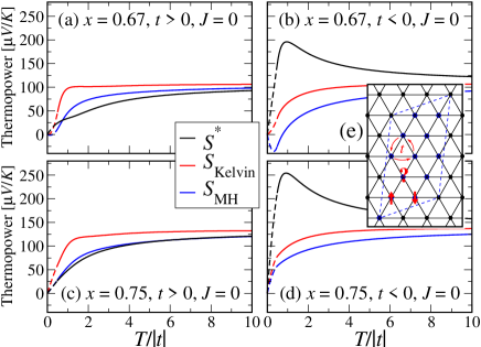
Figure 1: Thermopower vs. $T$ for the $t$-$J$ model (with $J=0$) corresponding to NCO in the Curie-Weiss metallic phase near $x\sim 0.7$. (a) and (c) correspond to $x=0.67$ and $x=0.75$ for the NCO system ($t>0$) while in (b) and (d) the sign of the hopping has been switched to investigate the enhancement expected for frustrated systems. The black, red (light gray), and blue (dark gray) lines are $S^{*}$, $S_{\mathrm{Kelvin}}$, and $S_{\mathrm{MH}}$. Finite size effects at low $T$ are treated in the spirit described previously mrp-joh-bss-prl-prbs . At each $x$, for $T$ below an appropriately chosen cutoff temperature $T_{0}=0.5|t|$, the thermopower is fit to $S(T)\to aT+bT^{2}$ where $a$ and $b$ are obtained from the computed $S(T_{0})$ and $S^{\prime}(T_{0})$ providing a sensible extrapolation to low $T$ and plotted as dashed lines. The inset figure (e) depicts the 12-site unit cell.

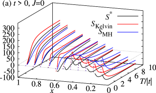
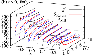
Figure 2: The thermopower vs. $T$ and $x$ for the $t$-$J$ model (with $J=0$) for $t>0$ (a) and $t<0$ (b). Note that $x\sim 0.7$ corresponds to the Curie-Weiss metallic phase of NCO, cf. Fig. 1. The line-type and color-coding is the same as in Fig. 1. Note that for dopings below 0.5 it is not clear whether the $t$-$J$ model adequately describes the physics of NCO.

$S^{*}$ adequately describes the physics of NCO for $x>0.5$ and, in particular the so-called Curie-Weiss metallic phase mrp-joh-bss-prl-prbs near $x\sim 0.7$. The subject of this work, however, is $S_{\mathrm{Kelvin}}$. We see in Figs. 1a and c and  2a, similar to $S_{\mathrm{MH}}$, $S_{\mathrm{Kelvin}}$ does a good job capturing the physics with minimal computational effort. However, $S_{\mathrm{Kelvin}}$ does seem to overestimate the thermopower for intermediate temperatures and high dopings as compared to $S_{\mathrm{MH}}$. Near $x\approx 0.7$, $S_{\mathrm{Kelvin}}$ and $S_{\mathrm{MH}}$ are similar but as $x$ is decreased the two formulae diverge and for low dopings, $S_{\mathrm{Kelvin}}$ better captures the physics as it is closer to the more accurate high frequency limit $S^{*}$.

An interesting property of the triangular lattice underlying the physics of NCO is its geometrical frustration frustration , cf. inset Fig. 1e. It was predicted bss-prb ; mrp-joh-bss-prl-prbs that if the sign of the hopping amplitude were flipped to $t<0$ the thermopower would be enhanced at low to intermediate $T$. We have considered this situation in Figs. 1b and d and 2b. Since the thermopower enhancement for $t<0$ compared to $t>0$ is largely a consequence of electron-electron interaction it is important to determine whether this effect is captured by $S_{\mathrm{Kelvin}}$. We see this enhancement is captured to some extent by $S_{\mathrm{Kelvin}}$ and $S_{\mathrm{Kelvin}}$ is better than $S_{\mathrm{MH}}$ in the large doping region where the enhancement is the greatest, but is missing some of the electron-electron physics at very low $T$ that is captured by $S^{*}$ (as is $S_{\mathrm{MH}}$).

III.4 FQHE at $\nu=5/2$

We now discuss how $S_{\mathrm{Kelvin}}$ is applied to dissipation-less systems such as the FQHE where thermopower can be used as a possible non-Abelian quasiparticle detector yang-halperin .

For a weakly disordered electron system (from Eq. (10) and (11)) $S_{\mathrm{Kelvin}}$ essentially gives the dissipation-less thermopower where particle velocities are further approximated. If the system is dissipation-less and the particle velocities are also energy independent, such as the FQHE, then we expect $S_{\mathrm{Kelvin}}$ is exact. An expression for the thermopower in a 2D electron system in the presence of a perpendicular magnetic field (the FQHE system) has been derived obraztsov-cooper ; yang-halperin , assuming zero impurities, as $\frac{{\mathcal{S}}}{q_{e}N}$ (Eq. (6) in Ref. yang-halperin, ). Yang and Halperin show yang-halperin that ${\mathcal{S}}\sim k_{B}N\log(d)$ where $d>1$ is the quantum dimension of the quasiparticles for the FQHE at $\nu=5/2$ (provided they are non-Abelian). Thus, a non-zero entropy linear in $N$ is obtained. From Eq. (8), we see that the thermopower is the derivative of the entropy with respect to the number of particles at constant $T$ and $V$. When entropy is linear in particle number, as in non-Abelian FQHE states, $\partial{\mathcal{S}}/\partial N\rightarrow{\mathcal{S}}/N$ and the formulas are identical. Our derivation provides a simple and straightforward insight into the formula given previously yang-halperin .

III.5 High Temperature Superconductors

Before concluding, we point out an intriguing application of $S_{\mathrm{Kelvin}}$ for high $T_{c}$ superconductors. For different families of high $T_{c}$ compounds, a universal curve of the thermopower, at $T=290K$, as a function of hole concentration $p\sim 1-n$ has been observed tallon-honma . The thermopower, in all families, vanishes near optimal doping ($p\sim 0.16$) starting out positive at small $p$. Phillips et al. phillips appeal to the atomic limit of $S_{\mathrm{MH}}$ as an explanation. Viewing this data  tallon-honma more generally, through the prism of $S_{\mathrm{Kelvin}}$ (Eq. (8)) we conclude that the optimal filling, i.e., maximum $T_{c}$, additionally corresponds to a local maximum of the electronic entropy as a function of filling. This conclusion is powerful, since we avoided the difficult issue of calculating either thermopower or entropy, merely using the link between them provided by $S_{\mathrm{Kelvin}}$.

IV Conclusion

It is clear that $S_{\mathrm{MH}}$, which has served as a virtual workhorse for years, has a new competitor in $S_{\mathrm{Kelvin}}$. This simple minded approximation can be written in closed form and in many difficult regimes, where the exact Kubo-Onsager expressions are not useful, and $S_{\mathrm{Kelvin}}$ provides an excellent guide to the physics of the system.

We acknowledge support from DOE-BES Grant No. DE-FG02-06ER46319 at UCSC, and MRP acknowledges support from LPS-CMTC at University of Maryland and Microsoft Project Q.

References

- (1) I. Terasaki, Y. Sasago, and K. Uchinokura, Phys. Rev. B 56, R12685 (1997); Y. Wang et al, Nature 423, 425 (2003); M. L. Foo et al, Phys. Rev. Lett. 92, 247001 (2004).
- (2) J. O. Haerter, M. R. Peterson, and B. S. Shastry, Phys. Rev. Lett. 97, 226402 (2006); M. R. Peterson, B. S. Shastry, and J. O Haerter, Phys. Rev. B. 76, 165118 (2007); J. O. Haerter, M. R. Peterson, and B. S. Shastry, ibid. 74, 245118 (2006).
- (3) A. P. Ramirez, in More is Different, edited by N. P. Ong and R. N. Bhatt (Princeton University Press, New Jersey, 2001).
- (4) B. S. Shastry, Phys. Rev. B. 73, 085117 (2006).
- (5) K. Yang and B. I Halperin, Phys. Rev. B. 79, 115317 (2009).
- (6) G. Moore and N. Read, Nucl. Phys. B 360, 362 (1991).
- (7) R. Willett et al., Phys. Rev. Lett. 59, 1776 (1987).
- (8) W. L. K Thomson, Proc. Roy. Soc. Edinburgh 123 Collected Papers I, pp. 237-41, (1854).
- (9) L. Onsager, Phys. Rev. 37, 405 (1931); ibid. 38, 2265 (1931).
- (10) R. Kubo, J. Phys. Soc. Jpn. 12, 570 (1957).
- (11) B. S. Shastry, Rep. Prog. Phys. 72, 016501 (2009).
- (12) Y. N. Obraztsov, Fiz. Tverd. Tela (Leningrad) 7, 573 (1965) [Sov. Phys. Solid State 7, 455 (1965)]; N. R. Cooper, B. I. Halperin, and I. M.Ruzin, Phys. Rev. B 55, 2344 (1997).
- (13) J. M. Luttinger, Phys. Rev. 135, A1505 (1964); ibid. 136, A1481 (1964).
- (14) S. Edwards, Phil. Mag. 3, 33, 1020 (1958).
- (15) P. M. Chaikin, and G. Beni, Phys. Rev. B 13, 647 (1976); R. R. Heikes, Thermoelectricity (Wily-Interscience, New York, 1961).
- (16) L. Arsenault, B. S. Shastry, and A. M. Tremblay, In preparation. .
- (17) F. Assad, and M. Imada, Phys. Rev. Lett. 74, 3868 (1995).
- (18) T. Pruschke, D. L. Cox, and M. Jarrell, Phys. Rev. B 47, 3553 (1993).
- (19) S. Obertelli, , J. R. Cooper, , and J. L Tallon. Phys. Rev. B 46, 14928 (1992); T. Honma and P. H. Hor, ibid. 77, 184520 (2008).
- (20) P. Phillips, T.-P. Choy, and R. G. Leigh, Rep. Prog. Phys. 72, 036501 (2009).