Spin Correlation Effects in
Top Quark Pair Production at the LHC

Abstract

At a 14 TeV proton-proton collider, the Large Hadron Collider (LHC), we show that top quark pair production is dominated at low invariant mass by the fusion of two like-helicity gluons, producing top quark pairs in the left-left or right-right helicity configurations. Whereas, at higher invariant mass the production is dominated by the fusion of unlike-helicity gluons, producing top quark pairs in the up-down or down-up off-diagonal configurations, identical to top quark pair production via quark-antiquark annihilation. We study in detail the low invariant mass region, and show that the spin correlations can be easily observed in this region by looking at the distribution of the difference in the azimuthal angles, $\Delta\phi$, of the dileptons decay products of the top quarks in the laboratory frame. Due to the large cross section for top pair production at the LHC, even with a cut requiring that the invariant mass of the top quark pair be less than 400 GeV, the approximate yield would be $10^{4}$ di-lepton (e, $\mu$) events per fb^-1 before detector efficiencies are applied. Therefore, there is ample statistics to form the $\Delta\phi$ distribution of the dilepton events, even with the invariant mass restriction. We also discuss possibilities for observing these spin correlations in the lepton plus jets channel.

I Introduction

Since the discovery of the top quark with a mass between 150 and 200 GeV by the CDF and D0 experiments at Fermilab in 1995, numerous authors, see mahlon and parke –Bernreuther:2004jv , have asked the question “Can the spin correlations in top quark pair production be observed?” This is a valid question since the top quark lifetime in the Standard Model is very short compared to the spin de-correlation time for such a heavy quark. In particular, $\Gamma_{T}\sim G_{F}m_{t}^{3}>>\Lambda^{2}_{QCD}/m_{t}$ where $\Gamma_{T}$ is the total width of the top quark, $m_{t}$ is mass of top quark, $G_{F}$ is the Fermi constant and $\Lambda_{QCD}$ is the QCD scale, thus the top quark decays before QCD interactions have the opportunity to appreciably affect its spin. The angular distribution of the top quark decay products in $t\rightarrow W^{+}+b$ followed by $W^{+}\rightarrow l^{+}+\nu$ or $\bar{d}+u$ are correlated with the top spin axis as follows:

$$\frac{1}{\Gamma_{T}}\frac{d\Gamma}{d\cos\chi_{i}}=(1+\alpha_{i}\cos\chi_{i})/2\quad\alpha_{i}=\left\{\begin{array}[]{l}+1.0\quad\hbox{$l^{+}$ or $\bar{d}$-quark}\\ -0.31\quad\hbox{$\bar{\nu}$ or $u$-quark}\\ -0.41\quad\hbox{$b$-quark}\end{array}\right.$$ (4)

where $\chi_{i}$ is the angle between the $i$-th decay product and the top quark spin axis in the top quark rest frame. Clearly, the charged lepton or $d$-quark coming from the decay of the $W$-boson are the most correlated with the top quark spin axis. For the anti-top, the signs of the $\alpha_{i}$ coefficients are flipped. Thus, if the spins of the top are correlated in top quark pair production and since the decay products of the tops are correlated with the spins then the decay products of the two top quarks are correlated. Since there is no net polarization of the top quarks, at least to leading order, the correlation between the $i$-th decay product of the top and $\bar{\imath}$-th decay product of the anti-top can be expressed by

$$\frac{1}{\sigma_{T}}\frac{d^{2}\sigma}{d\cos\chi_{i}d\cos\bar{\chi}_{\bar{i}}}=\frac{1}{4}(1+C_{t\bar{t}}~{}\alpha_{i}~{}\bar{\alpha}_{\bar{i}}~{}\cos\chi_{i}\cos\bar{\chi}_{\bar{i}}).$$ (5)

with

$$C_{t\bar{t}}\equiv\frac{\sigma_{\uparrow\uparrow}+\sigma_{\downarrow\downarrow}-\sigma_{\uparrow\downarrow}-\sigma_{\downarrow\uparrow}}{\sigma_{\uparrow\uparrow}+\sigma_{\downarrow\downarrow}+\sigma_{\uparrow\downarrow}+\sigma_{\downarrow\uparrow}}.$$ (6)

$\sigma_{\uparrow/\downarrow~{}\uparrow/\downarrow}$ is the production cross section for top quark pairs where the top quark has spin up or down with respect to the top spin axis and the anti-top has spin up or down with respect to the antitop spin axis. Clearly, the right choice for the spin axes of the top quark pair is important since a poor choice of spin axes can lead to a small value for the correlation parameter, $C_{t\bar{t}}$ and hence to small correlations between the decay products of the top and the antitop. For some processes, e.g. $q\bar{q}\rightarrow t\bar{t}$, there exist spin axis choices such that the correlation parameter, $C_{t\bar{t}}$, is maximal. However, even with these optimal choices, to observe the correlations one has to measure the angles $\chi_{i}$ and $\bar{\chi}_{\bar{\imath}}$ between the decay products and the spin axes in the rest frame of the top and antitop quarks respectively. To do this one has to reconstruct the top and the antitop rest frames; this is very challenging at a hadron collider. An obvious question is “Are there variables that carry the signature of the spin correlations which can be measured in the laboratory frame?” For $q\bar{q}\rightarrow t\bar{t}$ no such variables have been found that show a significant difference between full spin correlations and no spin correlations.

It has been known for some time that the spin correlations at the LHC are described very well by the helicity basis at low top-antitop invariant mass, whereas at higher invariant mass, counter to one’s naïve expectation, the spin correlations are degraded in the helicity basis. In this paper we explain this phenomenon by showing that at low invariant mass top quark pair production is dominated by like-helicity gluons, producing top quark pairs in the left-left or right-right helicity configuration, independent of the invariant mass. Whereas, at higher invariant mass top quark pair production is dominated by unlike-helicity gluons, producing top quark pairs in the up-down or down-up off-diagonal configuration, identical to that of top quark pair production via quark-antiquark annihilation. At ultra-high invariant masses, the up-down and down-up off-diagonal configurations become the familiar left-right or right-left helicity configurations; however, at the LHC only a small fraction of the total number of produced top pair events are in this ultra-high invariant mass region. The fact that the contributions from like and unlike helicity gluons impart different spin correlations to the top quark pairs makes $gg\rightarrow t\bar{t}$, which dominates top quark pair production at the LHC, a much richer process for analysis than the dominant Tevatron mechanism $q\bar{q}\rightarrow t\bar{t}$.

We study the low invariant mass region in detail. In this region, the like-helicity gluons dominate the production. We show that the spin correlations can be easily observed in this region by looking at the distribution of the difference in the azimuthal angles, $\Delta\phi$, of the dilepton decay products of the top quarks. For top quark pairs with an invariant mass $\leq 400$ GeV, the spin correlations give a 40% enhancement of this distribution at small angles ($\Delta\phi\approx 0$) and a 40% suppression of this distribution at large angles ($\Delta\phi\approx\pi$) compared to if there were no correlations between the production and decay of the top quarks. About 20% ($\sim 200$ pb) of the total next-to-leading order top-antitop quark production cross section passes this invariant mass cut so even in the di-lepton channel there are large numbers of events available to measure this distribution: about $10^{4}$ events per fb^-1 before detector efficiencies are applied.

The outline of this paper is as follows: in Sect. II we review what is known about the spin correlations for $q\bar{q}\rightarrow t\bar{t}$ before taking a closer look at the spin correlations for $gg\rightarrow t\bar{t}$ in Section III. Section IV addresses the question of how the top quark pair events at the LHC populate the scattering angle versus invariant mass plane. In Section V we add the decays of the top quarks. In Sect. VI we address the issue of which angular distributions are sensitive to the presence or absence of angular correlations among the $t\bar{t}$ decay products. We show that at low invariant mass the difference in the azimuthal angle of the charged leptons carries the signature of spin correlations in the laboratory frame. We also discuss possibilities for observing these spin correlations in the lepton plus jets channel. We summarize our conclusions in Sec. VII. Lastly, we include an Appendix which outlines the highly efficient method used in this paper for calculating the spin amplitudes. It can be applied to any $2\rightarrow 2$ process with arbitrary spins of the final state particles.

II Review of $q\bar{q}\rightarrow t\bar{t}$

II.1 Spin Amplitudes in an Arbitrary Basis

For a massive particle with momentum, $t$, and spin vector, $s_{t}$, the following relationships are satisfied

$$t^{2}=m_{t}^{2},\quad s_{t}^{2}=-1,\quad{\rm and}\quad t\cdot s_{t}=0.$$ (7)

The spin vector $s_{t}$ is most conveniently defined in the rest frame of the massive particle; in this frame it only can have spatial components. Thus, for top-antitop quark pair production via quark-antiquark annihilation or gluon-gluon fusion, we define the spin vector $s_{t}$ in the rest frame of the top quark. Since CP is conserved at tree level for this process, we restrict the spin vector to be in the scattering plane. It is convenient to measure the direction of spin vector $s_{t}$ with respect to the antitop quark or recoil direction. Thus we define the unit vector $s_{t}$ such that its direction is at an angle $\xi$, measured clockwise with respect to the antitop quark direction (see Fig. 1).

For the antitop quark we proceed in a similar fashion in defining $s_{\bar{t}}$. Here, instead of using the same angle $\xi$ to specify the direction of the spin vector with respect to the recoil direction, we use a different angle $\xi^{\prime}$. This allows for the independent manipulation of the antitop and top quark spins at intermediate steps. However, in the end, we will set $\xi^{\prime}=\xi$: then, in the zero momentum frame (ZMF), the spin vectors of the top and antitop quark are back-to-back as expected from the symmetry arguments.

It is particularly convenient to use the following combinations of $t$ and $s_{t}$ as follows:

$$t_{1}\equiv(t+m_{t}s_{t})/2,\quad{\rm and}\quad t_{2}\equiv(t-m_{t}s_{t})/2.$$ (8)

These satisfy

$$t_{1}^{2}=t_{2}^{2}=0,\quad t=t_{1}+t_{2},\quad{\rm and}\quad 2t_{1}\cdot t_{2}=m_{t}^{2}.$$ (9)

($\bar{t}_{1}$ and $\bar{t}_{2}$ are defined similarly for the antitop quark.) Since $t_{1}$ and $t_{2}$ are light-like vectors, the full power of the spinor helicity method can be used in evaluating the amplitudes as discussed in Ref. Mangano:1990by , resulting in many simplifications. For example, the Dirac spinor for a massive fermion with spin up can be written as, see Kleiss:1985yh

$$U_{\uparrow}(t)=\frac{1+\gamma_{5}}{2}U(t_{1})+e^{i\Psi}\frac{1-\gamma_{5}}{2}U(t_{2}).$$ (10)

This factorization into chiral components, with one depending only on $t_{1}$ and other only $t_{2}$ (apart from the phase factor $e^{i\Psi}\equiv\bar{U}(t_{2})\frac{1+\gamma_{5}}{2}U(t_{1})/m_{t}$), is particularly useful. For our purposes in this paper we need only two such spinors: a $\bar{U}_{\uparrow}$ spinor for the top quark, and a $V_{\uparrow}$ spinor for the antitop quark. These are given in spinor helicity notation by

$$\bar{U}_{\uparrow}(t) =\langle t_{1}+|+\displaystyle\frac{\langle t_{1}+|t_{2}-\rangle}{m_{t}}\langle t_{2}-| =\frac{1}{m_{t}}~{}\langle t_{1}+|(t+m_{t})$$

$$V_{\uparrow}(\bar{t}) =|\bar{t}_{1}-\rangle-|\bar{t}_{2}+\rangle\displaystyle\frac{\langle\bar{t}_{2}+|\bar{t}_{1}-\rangle}{m_{t}} =(m_{t}-\bar{t})|\bar{t}_{1}-\rangle~{}\frac{1}{m_{t}}$$ (11)

The full set of spinors for massive fermions may be found in Ref. mahlon and parke . In this paper we will show that once you have the amplitudes for $gg\rightarrow t_{\uparrow}\bar{t}_{\uparrow}$ in terms of the spin angles $\xi$ and $\xi^{\prime}$, you can obtain all of the other spin combinations for the top and antitop by simple algebraic manipulations.

Figure 1: Spin vector for top quark pair production. The direction of the top quark spin vector $s_{t}$ is given by the angle $\xi$ in this frame, measured in the clockwise direction from the recoil direction. The inset illustrates the situation in the ZMF, where the top and antitop are produced back-to-back and the scattering angle $\theta$ from the incoming beam direction.

II.2 Review of the Spin Structure of $q\bar{q}\rightarrow t\bar{t}$

The spinor structure of the matrix element for $q_{R}\bar{q}_{L}\rightarrow t\bar{t}$ can easily be shown to be of the form

$$\bar{U}(t)\{|q+\rangle\langle\bar{q}+|+|\bar{q}-\rangle\langle q-|\}V(\bar{t})$$ (12)

by using the Fierz identities on the current-current structure of the matrix element given by the standard Feynman rules. This can be used to recover the well-known tree level matrix element squared for $q_{R}\bar{q}_{L}\rightarrow t\bar{t}$ (see Ref. Parke:1996pr ):

$$|{\cal A}(q_{R}\bar{q}_{L}\rightarrow t_{\uparrow}\bar{t}_{\uparrow}\quad{\rm and}\quad t_{\downarrow}\bar{t}_{\downarrow})|^{2} = |{\cal A}(q_{L}\bar{q}_{R}\rightarrow t_{\uparrow}\bar{t}_{\uparrow}\quad{\rm and}\quad t_{\downarrow}\bar{t}_{\downarrow})|^{2}$$

$$\sim (\gamma^{-1}\sin\theta\cos\xi-\cos\theta\sin\xi)^{2}$$

$$|{\cal A}(q_{R}\bar{q}_{L}\rightarrow t_{\uparrow}\bar{t}_{\downarrow}\quad{\rm or}\quad t_{\downarrow}\bar{t}_{\uparrow})|^{2} = |{\cal A}(q_{L}\bar{q}_{R}\rightarrow t_{\downarrow}\bar{t}_{\uparrow}\quad{\rm or}\quad t_{\uparrow}\bar{t}_{\downarrow})|^{2}$$ (13)

$$\sim (\gamma^{-1}\sin\theta\sin\xi+\cos\theta\cos\xi\mp 1)^{2}.$$

Here the same spin angle, $\xi$, has been used for both the top and antitop quarks. From this general result it is clear that there is a basis, defined by

$$\tan\xi=\gamma^{-1}\tan\theta,$$ (14)

which sets the $\uparrow\uparrow+\downarrow\downarrow$ component to identically zero for all $\beta$, leaving only the $\uparrow\downarrow+\downarrow\uparrow$ component. This basis was first identified by Parke and Shadmi in Ref. Parke:1996pr and has been called the off-diagonal basis. It interpolates between the beamline basis ($\cos\xi=\cos\theta$) at threshold, and the helicity basis ($\cos\xi=\pm 1$) in the ultra-relativistic limit. In the off-diagonal basis, Eq. (13) becomes

$$|{\cal A}(q_{R}\bar{q}_{L}\rightarrow t_{\uparrow}\bar{t}_{\uparrow}\enspace{\rm and}\enspace t_{\downarrow}\bar{t}_{\downarrow})|^{2}=|{\cal A}(q_{L}\bar{q}_{R}\rightarrow t_{\uparrow}\bar{t}_{\uparrow}\enspace{\rm and}\enspace t_{\downarrow}\bar{t}_{\downarrow})|^{2}=0$$

$$\enspace\thinspace|{\cal A}(q_{R}\bar{q}_{L}\rightarrow t_{\uparrow}\bar{t}_{\downarrow}\enspace{\rm or}\enspace t_{\downarrow}\bar{t}_{\uparrow})|^{2}=|{\cal A}(q_{L}\bar{q}_{R}\rightarrow t_{\downarrow}\bar{t}_{\uparrow}\enspace{\rm or}\enspace t_{\uparrow}\bar{t}_{\downarrow})|^{2}\sim\left(1\mp\sqrt{1-\beta^{2}\sin^{2}\theta}\right)^{2},$$

(15)

whereas the helicity basis is obtained by setting $\cos\xi=-1$; in this basis

$$|{\cal A}(q_{R}\bar{q}_{L}\rightarrow t_{R}\bar{t}_{R}\enspace{\rm and}\enspace t_{L}\bar{t}_{L})|^{2}=|{\cal A}(q_{L}\bar{q}_{R}\rightarrow t_{R}\bar{t}_{R}\enspace{\rm and}\enspace t_{L}\bar{t}_{L})|^{2}\sim\gamma^{-2}\sin^{2}\theta$$

$$\enspace\thinspace|{\cal A}(q_{R}\bar{q}_{L}\rightarrow t_{R}\bar{t}_{L}\enspace{\rm or}\enspace t_{L}\bar{t}_{R})|^{2}=|{\cal A}(q_{L}\bar{q}_{R}\rightarrow t_{L}\bar{t}_{R}\enspace{\rm or}\enspace t_{R}\bar{t}_{L})|^{2}\sim(1\pm\cos\theta)^{2}.$$ (16)

Clearly, for $\gamma>>1$, the helicity basis and the Off-Diagonal basis become identical. As we will see in the next section, the spin correlations for unlike-helicity gluons producing top quark pairs are identical to those in quark-antiquark annihilation.

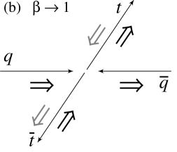
Figure 2: The spin configurations for the process $q_{R}\bar{q}_{L}\rightarrow t\bar{t}$ are best described by the off-diagonal basis which interpolates between the beamline basis at low $\beta$ to helicity at very high $\beta$ as given by Eq. 15. (a) is the limit $\beta\rightarrow 0$ where the top quark spins are aligned in the same direction as the incoming quark spins whereas (b) is the limit $\beta\rightarrow 1$ where the helicity state $t_{R}\bar{t}_{L}$ dominates for scattering angles less than 90 degrees. The relative probability of $t_{R}\bar{t}_{L}$ to $t_{L}\bar{t}_{R}$ is given by $(1+\cos\theta)^{2}:(1-\cos\theta)^{2}$.

III A Closer Look at $gg\rightarrow t\bar{t}$

The tree-level matrix element for $gg\rightarrow t\bar{t}$ can be factorized into two terms: one depending on the color factors and $t$ and $u$-channel propagators and the other depending on the the spin of the gluons and top quarks, as follows

$${\cal A}(g_{1}g_{2}\rightarrow t\bar{t})=ig^{2}_{s}\left\{\frac{[T^{a_{1}}T^{a_{2}}]_{\bar{\imath}i}}{(2t\cdot p_{1})}+\frac{[T^{a_{2}}T^{a_{1}}]_{\bar{\imath}i}}{(2t\cdot p_{2})}\right\}M(g_{1}g_{2}\rightarrow t\bar{t}).$$ (17)

The reduced matrix element $M(g_{1}g_{2}\rightarrow t\bar{t})$ is symmetric under the interchange of the two gluon momenta but depends on the the helicity of the gluons and the spin of the top and antitop quarks.

The square of the color-propogator factor, summed over the gluon and top quark colors, is given by

$$\sum_{color}\left|\frac{[T^{a_{1}}T^{a_{2}}]_{\bar{\imath}i}}{(2t\cdot p_{1})}+\frac{[T^{a_{2}}T^{a_{1}}]_{\bar{\imath}i}}{(2t\cdot p_{2})}\right|^{2}=\frac{4}{3}\thinspace\frac{4(t\cdot p_{1})^{2}+4(t\cdot p_{2})^{2}-(t\cdot p_{1})(t\cdot p_{2})}{(t\cdot p_{1})^{2}(t\cdot p_{2})^{2}}.$$ (18)

When evaluated in the ZMF, this sum reduces to the form

$$\sum_{color}\left|\frac{[T^{a_{1}}T^{a_{2}}]_{\bar{\imath}i}}{(2t\cdot p_{1})}+\frac{[T^{a_{2}}T^{a_{1}}]_{\bar{\imath}i}}{(2t\cdot p_{2})}\right|^{2}=\frac{{\cal Y}(\beta,c_{\theta})}{\gamma^{4}m_{t}^{4}},$$ (19)

with

$${\cal Y}(\beta,c_{\theta})=\frac{4}{3}\thinspace\frac{7+9\beta^{2}c^{2}_{\theta}}{(1-\beta^{2}c^{2}_{\theta})^{2}}.$$ (20)

In these expressions $\beta$ is the ZMF speed of the top quarks and $c_{\theta}$ is the cosine of the ZMF scattering angle $\theta$.

The reduced matrix element for on-mass-shell top quarks, $M(g_{1}g_{2}\rightarrow t\bar{t})$, is simply given by

$$M(g_{R}g_{L}\rightarrow t\bar{t}) = \frac{2~{}\langle p_{2}+|\thinspace t\thinspace|p_{1}+\rangle}{2p_{1}\cdot p_{2}}\thinspace\bar{U}(t)\{|p_{1}+\rangle\langle p_{2}+|+|p_{2}-\rangle\langle p_{1}-|\}V(\bar{t})$$ (21)

for unlike helicity gluons and by

$$M(g_{R}g_{R}\rightarrow t\bar{t}) = 2m_{t}\frac{\langle p_{1}-|p_{2}+\rangle}{\langle p_{1}+|p_{2}-\rangle}\thinspace\bar{U}(t)\gamma_{L}V(\bar{t})\quad{\rm where}\quad\gamma_{L,R}\equiv\frac{1}{2}(1\mp\gamma_{5})$$ (22)

for like-helicity gluons. Note the similarity in the spinor structure for $g_{R}g_{L}\rightarrow t\bar{t}$ and $q_{R}\bar{q}_{L}\rightarrow t\bar{t}$. Also, the spinor structure for $g_{R}g_{R}\rightarrow t\bar{t}$ is particularly simple, $\bar{U}(t)\gamma_{L}V(\bar{t})$; it contains no $s$-channel pole. In a later section of this paper, we use these two expressions to give a simple analytic expression for $gg\rightarrow t\bar{t}$ including the decay of the two top quarks. However, in the next section we will evaluate these expressions using the spinors for polarized top quarks given in Eq. (11).

III.1 Unlike-Helicity Gluons

For unlike-helicity gluons the reduced matrix element $M(g_{R}g_{L}\rightarrow t_{\uparrow}\bar{t}_{\uparrow})$ is given by

$$M(g_{R}g_{L}\rightarrow t_{\uparrow}\bar{t}_{\uparrow})=\frac{2\langle p_{2}+|t|p_{1}+\rangle}{m_{t}(2p_{1}\cdot p_{2})}\Bigl{\{}\langle t_{1}+|t_{2}|p_{1}+\rangle\langle p_{2}+|\bar{t}_{1}-\rangle{-}\langle t_{1}+|p_{2}-\rangle\langle p_{1}-|\bar{t}_{2}|\bar{t}_{1}-\rangle\Bigr{\}},$$

which, when evaluated in the ZMF using the spin vectors described in the previous section, becomes

$$M(g_{R}g_{L}\rightarrow t_{\uparrow}\bar{t}_{\uparrow}) \sim \beta\sin\theta\{(1-\cos\theta)\sin(\xi/2)\cos(\xi{{}^{\prime}}/2)-(1+\cos\theta)\cos(\xi/2)\sin(\xi{{}^{\prime}}/2)$$ (24)

$$\enspace\quad\quad+\gamma^{-1}\sin\theta[\cos(\xi/2)\cos(\xi{{}^{\prime}}/2)-\sin(\xi/2)\sin(\xi{{}^{\prime}}/2)]\}.$$

Here the coefficients in front of the products of the $\xi$-dependent trigonometric functions are the appropriate helicity amplitudes whereas the products of the $\xi$-dependent trigonometric functions themselves are products of Wigner $d$-functions (see Appendix A). The relative signs between the various components of these expressions are important and care must be taken to make sure they are correct.

Using a different spin angle for the $t$ and $\bar{t}$ allows for manipulation of the spin of the top independent of the antitop and vice versa. Thus, all of the spin amplitudes for $g_{R}g_{L}\rightarrow t\bar{t}$ can be simply obtained from $g_{R}g_{L}\rightarrow t_{\uparrow}\bar{t}_{\uparrow}$ as follows:

$$|M_{\downarrow\uparrow}(\xi,\xi^{\prime})|=|M_{\uparrow\uparrow}(\xi\pm\pi,\xi^{\prime})|=\left|\left(\displaystyle\frac{d}{d\xi/2}\right)M_{\uparrow\uparrow}(\xi,\xi^{\prime})\right|$$ (25)

$$|M_{\uparrow\downarrow}(\xi,\xi^{\prime})|=|M_{\uparrow\uparrow}(\xi,\xi^{\prime}\pm\pi)|=\left|\left(\displaystyle\frac{d}{d\xi{{}^{\prime}}/2}\right)M_{\uparrow\uparrow}(\xi,\xi^{\prime})\right|$$ (26)

$$|M_{\downarrow\downarrow}(\xi,\xi^{\prime})|=|M_{\uparrow\uparrow}(\xi\pm\pi,\xi^{\prime}\pm\pi)|=\left|\left(\displaystyle\frac{d}{d\xi/2}\right)\left(\displaystyle\frac{d}{d\xi^{\prime}/2}\right)M_{\uparrow\uparrow}(\xi,\xi^{\prime})\right|.$$ (27)

Flipping the spin of a particle is accomplished by one of two equivalent methods:

• Addition or subtraction of $\pi$ from the spin angle $\xi$.

• Differentiation of the amplitude with respect to $\xi/2$.

A detailed discussion with examples of how to use these techniques for arbitrary spins is given in Appendix A.

At this stage we can make the spin axes of the top quark pair back-to-back in the ZMF by setting $\xi^{{}^{\prime}}=\xi$. Thus, for unlike-helicity gluons we obtain

$$|{\cal A}(g_{R}g_{L}\rightarrow t_{\uparrow}\bar{t}_{\uparrow}\enspace{\rm and}\enspace t_{\downarrow}\bar{t}_{\downarrow})|^{2} = {\cal Y}(\beta,\theta)~{}\beta^{2}\sin^{2}\theta(\gamma^{-1}\sin\theta\cos\xi-\cos\theta\sin\xi)^{2},$$ (28)

$$|{\cal A}(g_{R}g_{L}\rightarrow t_{\uparrow}\bar{t}_{\downarrow}\enspace{\rm or}\enspace t_{\downarrow}\bar{t}_{\uparrow})|^{2} = {\cal Y}(\beta,\theta)~{}\beta^{2}\sin^{2}\theta(\gamma^{-1}\sin\theta\sin\xi+\cos\theta\cos\xi\mp 1)^{2},$$ (29)

and

$$|{\cal A}(g_{L}g_{R}\rightarrow t_{\uparrow}\bar{t}_{\uparrow}\enspace{\rm and}\enspace t_{\downarrow}\bar{t}_{\downarrow})|^{2} = |{\cal A}(g_{R}g_{L}\rightarrow t_{\uparrow}\bar{t}_{\uparrow}\enspace{\rm and}\enspace t_{\downarrow}\bar{t}_{\downarrow})|^{2},$$ (30)

$$|{\cal A}(g_{L}g_{R}\rightarrow t_{\downarrow}\bar{t}_{\uparrow}\enspace{\rm or}\enspace t_{\uparrow}\bar{t}_{\downarrow})|^{2} = |{\cal A}(g_{R}g_{L}\rightarrow t_{\uparrow}\bar{t}_{\downarrow}\enspace{\rm or}\enspace t_{\downarrow}\bar{t}_{\uparrow})|^{2},$$ (31)

with

$$\sum_{\rm all}|{\cal A}(g_{R}g_{L}\rightarrow t\bar{t})|^{2}=\sum_{\rm all}|{\cal A}(g_{L}g_{R}\rightarrow t\bar{t})|^{2} = 2~{}{\cal Y}(\beta,\theta)~{}\beta^{2}\sin^{2}\theta(2-\beta^{2}\sin^{2}\theta).$$ (32)

As in $q\bar{q}\rightarrow t\bar{t}$, a great simplification occurs for the off-diagonal basis Parke:1996pr , $\tan\xi=\gamma^{-1}\tan\theta$, where

$$|{\cal A}(g_{L}g_{R}\rightarrow t_{\uparrow}\bar{t}_{\uparrow}\enspace{\rm and}\enspace t_{\downarrow}\bar{t}_{\downarrow})|^{2}=|{\cal A}(g_{R}g_{L}\rightarrow t_{\uparrow}\bar{t}_{\uparrow}\enspace{\rm and}\enspace t_{\downarrow}\bar{t}_{\downarrow})|^{2}=0.$$ (33)

The off-diagonal basis is the basis that interpolates from the beamline basis at threshold to the helicity bases at ultra-relativistic energies for the $q\bar{q}\rightarrow t\bar{t}$ process. Thus, for unlike-helicity gluons we have a very similar situation to that of $q\bar{q}\rightarrow t\bar{t}$: the only non-zero amplitudes are given by

$$|{\cal A}(g_{R}g_{L}\rightarrow t_{\uparrow}\bar{t}_{\downarrow}\enspace{\rm or}\enspace t_{\downarrow}\bar{t}_{\uparrow}|^{2} = |{\cal A}(g_{L}g_{R}\rightarrow t_{\downarrow}\bar{t}_{\uparrow}\enspace{\rm or}\enspace t_{\uparrow}\bar{t}_{\downarrow}|^{2}$$ (34)

$$= {\cal Y}(\beta,\theta)~{}\beta^{2}\sin^{2}\theta\left(1\mp\sqrt{1-\beta^{2}\sin^{2}\theta}\right)^{2},$$

as illustrated in Fig. 3.

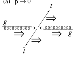
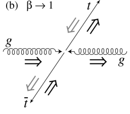
Figure 3: The spin configurations for the process $g_{R}g_{L}\rightarrow t\bar{t}$ are best described by the off-diagonal basis, which interpolates between the beamline basis at low $\beta$ and the helicity basis at very high $\beta$ (see Eq. 34). As far as the spins of the top quarks are concerned, this process, $g_{R}g_{L}\rightarrow t\bar{t}$, is identical to top quark production via quark-antiquark collisions, $q_{R}\bar{q}_{L}\rightarrow t\bar{t}$, see Fig. 2. (a) illustrates the limit $\beta\rightarrow 0$ where the top quark spins are aligned in the same direction as the incoming gluon spins whereas (b) illustrates the limit $\beta\rightarrow 1$ where the helicity state $t_{R}\bar{t}_{L}$ dominates for scattering angles less than 90 degrees. The relative probability of $t_{R}\bar{t}_{L}$ to $t_{L}\bar{t}_{R}$ is given by $(1+\cos\theta)^{2}:(1-\cos\theta)^{2}$.

III.2 Like-Helicity Gluons

For like-helicity gluons the reduced matrix element $M(g_{R}g_{R}\rightarrow t_{\uparrow}\bar{t}_{\uparrow})$ is simply given by the following combination of spinor products

$$M(g_{R}g_{R}\rightarrow t_{\uparrow}\bar{t}_{\uparrow})=2m_{t}\frac{\langle p_{1}-|p_{2}+\rangle}{\langle p_{1}+|p_{2}-\rangle}\langle t_{1}+|\bar{t}_{1}-\rangle,$$ (35)

which when evaluated in the ZMF using the spin vectors described in the previous section is just

$$M(g_{R}g_{R}\rightarrow t_{\uparrow}\bar{t}_{\uparrow}) \sim \gamma^{-1}\{(1-\beta)\cos(\xi/2)\cos(\xi{{}^{\prime}}/2)+(1+\beta)\sin(\xi/2)\sin(\xi{{}^{\prime}}/2)\}.$$ (36)

Treating these expressions in a manner similar to the unlike-helicity case discussed in the previous section we obtain

$$|{\cal A}(g_{R}g_{R}\rightarrow t_{\uparrow}\bar{t}_{\uparrow}\enspace{\rm or}\enspace t_{\downarrow}\bar{t}_{\downarrow})|^{2}={\cal Y}(\beta,\theta)~{}\gamma^{-2}(1\mp\beta\cos\xi)^{2},$$ (37)

$$|{\cal A}(g_{R}g_{R}\rightarrow t_{\uparrow}\bar{t}_{\downarrow}\enspace{\rm and}\enspace t_{\downarrow}\bar{t}_{\uparrow})|^{2}={\cal Y}(\beta,\theta)~{}\gamma^{-2}\beta^{2}\sin^{2}\xi.$$ (38)

Similarly, it is easy to show that for left-handed like-helicity gluons

$$|{\cal A}(g_{L}g_{L}\rightarrow t_{\downarrow}\bar{t}_{\downarrow}\enspace{\rm or}\enspace t_{\uparrow}\bar{t}_{\uparrow})|^{2} = |{\cal A}(g_{R}g_{R}\rightarrow t_{\uparrow}\bar{t}_{\uparrow}\enspace{\rm or}\enspace t_{\downarrow}\bar{t}_{\downarrow})|^{2},$$ (39)

$$|{\cal A}(g_{L}g_{L}\rightarrow t_{\uparrow}\bar{t}_{\downarrow}\enspace{\rm and}\enspace t_{\downarrow}\bar{t}_{\uparrow})|^{2} = |{\cal A}(g_{R}g_{R}\rightarrow t_{\uparrow}\bar{t}_{\downarrow}\enspace{\rm and}\enspace t_{\downarrow}\bar{t}_{\uparrow})|^{2}.$$ (40)

Summing over all of the final spins gives

$$\sum_{\rm all}|{\cal A}(g_{R}g_{R}\rightarrow t\bar{t})|^{2}=\sum_{\rm all}|{\cal A}(g_{L}g_{L}\rightarrow t\bar{t})|^{2}=2~{}{\cal Y}(\beta,\theta)~{}(1-\beta^{4}),$$ (41)

independent of the spin axis used for the top quarks.

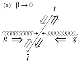
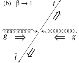
Figure 4: The spin configurations for the process $g_{R}g_{R}\rightarrow t\bar{t}$ are best described by the helicity basis for all $\beta$ (see Eq. 43). (a) illustrates the limit $\beta\rightarrow 0$ where the relative probability of $t_{R}\bar{t}_{R}$ to $t_{L}\bar{t}_{L}$ is $(1+\beta)^{2}:(1-\beta)^{2}$ whereas (b) illustrates the limit $\beta\rightarrow 1$ where $t_{R}\bar{t}_{R}$ completely dominates. For $g_{L}g_{L}\rightarrow t\bar{t}$, flip the spins on both the gluons and the top quarks.

Clearly, a great simplification occurs for like-helicity gluons if one uses the helicity basis ($\xi$=0 or $\pi$) for the top quarks. In the helicity basis

$$|{\cal A}(g_{L}g_{L}\rightarrow t_{R}\bar{t}_{L}\enspace{\rm and}\enspace t_{L}\bar{t}_{R})|^{2}=|{\cal A}(g_{R}g_{R}\rightarrow t_{R}\bar{t}_{L}\enspace{\rm and}\enspace t_{L}\bar{t}_{R})|^{2}=0$$ (42)

for all values of $\beta$. Conventional wisdom states that helicity provides a simple description for most processes only at ultra-relativistic energies. However, as illustrated in Fig. 4, $t\bar{t}$ production from like-helicity gluons is an exception to this expectation: in this case, the helicity basis provieds a simple description for all $\beta$, with the only non-zero amplitudes given by

$$|{\cal A}(g_{R}g_{R}\rightarrow t_{R}\bar{t}_{R}\enspace{\rm or}\enspace t_{L}\bar{t}_{L})|^{2}=|{\cal A}(g_{L}g_{L}\rightarrow t_{L}\bar{t}_{L}\enspace{\rm or}\enspace t_{R}\bar{t}_{R}|^{2}={\cal Y}(\beta,\theta)~{}\gamma^{-2}(1\pm\beta)^{2}.$$ (43)

Both the like and unlike gluon helicity amplitudes agree with those found in the appendix of Ref. hiroshima group .

III.3 Combining Like- and Unlike-Helicity Gluons

At the LHC we must combine the like-helicity and unlike-helicity gluon cases since there is no way to polarize the incoming gluons. By looking at Eqns. (29) and (38), it is clear that there is no basis which makes the top quark spins purely $\uparrow\uparrow+\downarrow\downarrow$ OR $\uparrow\downarrow+\downarrow\uparrow$ at the LHC because the constant term appears in $\uparrow\uparrow+\downarrow\downarrow$ for like-helicity gluons and $\uparrow\downarrow+\downarrow\uparrow$ for unlike-helicity gluons.

However, there are regions of the $(\cos\theta,\beta)$ plane for which one of the like-helicity gluon amplitude or the unlike-helicity amplitude dominates. Along the curve given by

$$\beta\gamma\sin\theta=1\hbox{ or, equivalently, }\beta^{2}=1/(2-\cos^{2}\theta)$$ (44)

the like-helicity and the unlike-helicity contribute equally to top quark pair production. On this curve

$$\sum_{\rm all}|{\cal A}(g_{R}g_{R}\rightarrow t\bar{t})|^{2}=\sum_{\rm all}|{\cal A}(g_{L}g_{L}\rightarrow t\bar{t})|^{2}=\sum_{\rm all}|{\cal A}(g_{R}g_{L}\rightarrow t\bar{t})|^{2}=\sum_{\rm all}|{\cal A}(g_{L}g_{R}\rightarrow t\bar{t})|^{2}.$$

In the region $\beta\gamma\sin\theta<1$ the like-helicity gluon amplitudes dominate the cross section, whereas in the region $\beta\gamma\sin\theta>1$ the unlike-helicity gluon amplitudes dominate the cross section. Thus, it is clear that one should use the helicity basis when $\beta\gamma\sin\theta<<1$ and the off-diagonal basis when $\beta\gamma\sin\theta>>1$. In the next section we will optimize the basis choice to maximize the spin correlations in the intermediate region, $\beta\gamma\sin\theta\sim 1$.

III.4 Optimizing the Choice of Spin Basis

For unpolarized gluons, the fraction of top quark pair events at a given point in the $(\cos\theta,\beta)$ plane that have $\uparrow\uparrow$ or $\downarrow\downarrow$ spins is

$$f(\theta,\beta) \equiv \frac{\sum_{\uparrow\uparrow+\downarrow\downarrow}|{\cal A}(gg\rightarrow t\bar{t})|^{2}}{\sum_{all}|{\cal A}(gg\rightarrow t\bar{t})|^{2}}$$

$$= \frac{\gamma^{-2}(1+\beta^{2}\cos^{2}\xi)+\beta^{2}\sin^{2}\theta(\gamma^{-1}\sin\theta\cos\xi-\cos\theta\sin\xi)^{2}}{((1-\beta^{4})+\beta^{2}\sin^{2}\theta(2-\beta^{2}\sin^{2}\theta))}.$$

It is a straightforward analytic exercise to find the extrema of this function with respect to the angle $\xi$. The maxima, $f_{\rm same}(\theta,\beta)$, gives the maximum fraction of $\uparrow\uparrow+\downarrow\downarrow$ whereas the minima, $f_{\rm oppo}(\theta,\beta)$, gives the minimum fraction of $\uparrow\uparrow+\downarrow\downarrow$ or, equivalently, the maximum fraction of $\uparrow\downarrow+\downarrow\uparrow$. These fractions are given by

$$f_{\{{\rm same,~{}oppo}\}}(\theta,\beta)\equiv$$ (45)

$$\frac{\gamma^{-2}+\frac{1}{2}\beta^{2}(\sin^{2}\theta\cos^{2}\theta+\gamma^{-2}\sin^{4}\theta+\gamma^{-2})\left\{1\pm\sqrt{1-\frac{(2\gamma^{-1}\cos\theta\sin\theta)^{2}}{(\sin^{2}\theta\cos^{2}\theta+\gamma^{-2}\sin^{4}\theta+\gamma^{-2})^{2}}}\right\}}{((1-\beta^{4})+\beta^{2}\sin^{2}\theta(2-\beta^{2}\sin^{2}\theta))}.$$

Both extrema occur when $\xi$ satisfies

$$\tan 2\xi_{\{{\rm same,~{}oppo}\}}=\frac{2\gamma^{-1}\sin^{3}\theta\cos\theta}{\sin^{2}\theta\cos^{2}\theta-\gamma^{-2}\sin^{4}\theta-\gamma^{-2}};$$ (46)

they are related as follows: $\xi_{\rm oppo}=\xi_{\rm same}+\pi/2$. The contours of $f_{\rm same}(\theta,\beta)$ in the $(\cos\theta,\beta^{2})$ plane are given by the solid lines in Fig. 5(a) whereas for $f_{\rm oppo}(\theta,\beta)$ see Fig. 5(b).

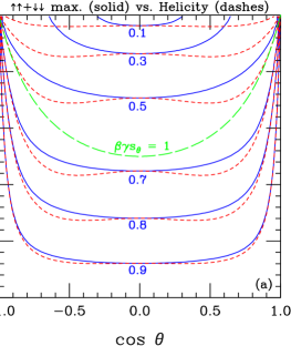
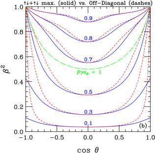
Figure 5: Panels (a) and (b) show, in the $(\cos\theta,\beta^{2})$ plane, the maximum fractions of $\uparrow\uparrow+\downarrow\downarrow$, $f_{\rm same}(\theta,\beta)$, and $\uparrow\downarrow+\downarrow\uparrow$, $f_{\rm oppo}(\theta,\beta)$, respectively (solid contours). In both panels the long-dashed line is $\beta\gamma\sin\theta=1$ or equivalently $\beta^{2}=1/(2-\cos^{2}\theta)$ below which the like-helicity gluons dominate and above the unlike-helicity gluons dominate. In (a) the short-dashed lines are the fractions of LL+RR top quark pairs in the helicity basis which below $\beta\gamma\sin\theta=1$ are close to the maximum fractions for $\uparrow\uparrow+\downarrow\downarrow$, $f_{\rm same}(\theta,\beta)$. Whereas in (b) the short-dashed lines are the fractions of $\uparrow\downarrow+\downarrow\uparrow$ in the Off-Diagonal basis which above $\beta\gamma\sin\theta=1$ are close to the maximum fractions of $\uparrow\downarrow+\downarrow\uparrow$, $f_{\rm oppo}(\theta,\beta)$.

At any given point in the $(\cos\theta,\beta^{2})$ plane, the basis which exhibits the strongest correlations is the one whose spin fraction has the largest difference from $\frac{1}{2}$. If $|f_{\rm oppo}(\theta,\beta)-1/2|$ is larger than $|f_{\rm same}(\theta,\beta)-1/2|$ then one should use $\xi_{\rm oppo}$; otherwise, $\xi_{\rm same}$ should be used. The condition that must be satisfied for both $f_{\rm same}(\theta,\beta)$ and $f_{\rm oppo}(\theta,\beta)$ to have equal difference (but opposite sign) from $1/2$ occurs when

$$f_{\rm same}(\theta,\beta)+f_{\rm oppo}(\theta,\beta)=1,\hbox{ or }\beta\gamma\sin\theta=1.$$ (47)

Not surprisingly this is the same curve that also separates the dominance of the contribution of like-helicity from unlike-helicity gluons. Thus, when $\beta\gamma\sin\theta<1$ the like-helicity gluons dominate and $\xi_{\rm same}$ should be used to maximize the $\uparrow\uparrow+\downarrow\downarrow$ fraction, whereas if $\beta\gamma\sin\theta>1$ the unlike-helicity gluons dominate and we should use $\xi_{\rm oppo}$ to maximize the $\uparrow\downarrow+\downarrow\uparrow$ fraction; this is equivalent to minimizing the $\uparrow\uparrow+\downarrow\downarrow$ fraction. The long-dashed line in both parts of Fig. 5 is the curve $\beta\gamma\sin\theta=1$; this is the demarkation curve between maximizing $\uparrow\uparrow+\downarrow\downarrow$ and maximizing $\uparrow\downarrow+\downarrow\uparrow$.

It is worthwhile asking the following two questions:

• In the region dominated by like-helicity gluons ($\beta\gamma\sin\theta<1$), how much does the maximum fraction of $\uparrow\uparrow+\downarrow\downarrow$ differ from what the helicity basis would give in the same region?

• In the region dominated by unlike-helicity gluons ($\beta\gamma\sin\theta>1$), how much does the maximum fraction of $\uparrow\downarrow+\downarrow\uparrow$ differ from what the off-diagonal basis would give in the same region?

These two questions are also addressed by Fig. 5. In (a) we have also plotted (short dashes) the fraction of top quark pairs which are LL+RR in the helicity basis and in (b) the fraction that are $\uparrow\downarrow+\downarrow\uparrow$ in the off-diagonal basis. Clearly, these figures indicate that the helicity basis does almost as well as the basis which maximizes $\uparrow\uparrow+\downarrow\downarrow$ for $\beta\gamma\sin\theta<1$ and that the off-diagonal basis does almost as well as the basis which maximizes $\uparrow\downarrow+\downarrow\uparrow$ for $\beta\gamma\sin\theta>1$.

Now that we understand the production dynamics for top quark pair production from gluon-gluon fusion we can turn to the question of what regions in the $(\cos\theta,\beta^{2})$ plane do the top quark pair events occur at the LHC.

IV Phenomenolgy of Top Quark Pair Production at the LHC

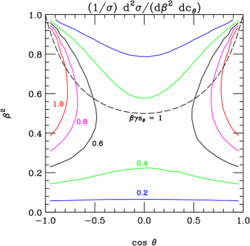
Figure 6: The differential cross section $(1/\sigma_{\rm tot})~{}d^{2}\sigma/d(\cos\theta)~{}d\beta^{2}$ for top quark pair production at the LHC assuming total beam energy of 14 TeV. The long-dashed line is $\beta\gamma\sin\theta=1$ (or $\beta^{2}=1/(2-\cos^{2}\theta)$) is the demarkation line for the differential cross section to be dominated by like-helicity gluons (below) and unlike-helicity gluons (above).

In Fig. 6 we plot the differential cross section

$$\frac{1}{\sigma_{\rm tot}}~{}\frac{d^{2}\sigma}{d(\cos\theta)d\beta^{2}}~{}(gg\rightarrow t\bar{t})$$

in the $(\cos\theta,\beta^{2})$ plane where $\sigma_{\rm tot}$ is the total cross section. This figure gives us the relative distribution of top quark pair events in this plane. A breakdown of the fraction of events for like- and unlike-helicity gluons broken into the appropriate regions in $\beta\gamma s_{\theta}$ are given in Table 1.

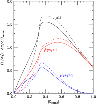
Figure 7: The differential distributions of $|C_{\rm same}|$, $(1/\sigma_{{}_{T}})~{}d\sigma/d|C_{\rm same}|$. The dashed curves are for the optimal basis, Eqn. (46), whereas the solid curves employ the helicity basis when $\beta\gamma s_{\theta}<1$ and the off-diagonal basis when $\beta\gamma s_{\theta}>1$. The mean values of $|C_{same}|$ for the different bases and regions are collected in Table 2.

Table 1: Fraction of $t\bar{t}$ events catagorized by the helicities of the initial state gluons and location in the $(\cos\theta,\beta^{2})$ plane at the LHC with $\sqrt{s}=14$ TeV.

	$\beta\gamma s_{\theta}<$1	$\beta\gamma s_{\theta}>$1	all
$gg$ Like	55%	10%	165%
$gg$ Unlike	20%	15%	135%
Total	75%	25%	100%

Fig. 7 shows the differential cross section with respect to $|C_{\rm same}|$, where

$$C_{\rm same}\equiv 2f_{\uparrow\uparrow+\downarrow\downarrow}-1\hbox{ and }C_{\rm oppo}\equiv 2f_{\uparrow\downarrow+\downarrow\uparrow}-1$$ (48)

are the quantities which control the size of the correlations for any given spin basis (note that $C_{\rm oppo}=-C_{\rm same}$). In this figure we have split up the contributions into two pieces: one for $\beta\gamma\sin\theta<1$ and the other for $\beta\gamma\sin\theta\geq 1$ . For $\beta\gamma\sin\theta<1$, we show the contribution in the basis which maximizes the $\uparrow\uparrow+\downarrow\downarrow$ component as well as the helicity basis; whereas for $\beta\gamma\sin\theta\geq 1$, we show the contribution in the basis which maximizes $\uparrow\downarrow+\downarrow\uparrow$ as well as the off-diagonal basis. This figure clearly shows that there are only small differences between using the best basis and the helicity basis for $\beta\gamma\sin\theta<1$ and the best basis and the off-diagonal basis for $\beta\gamma\sin\theta>1$.

At the LHC, the total top quark pair production cross section is $\sim$1 nb (at next-to-leading order) giving approximately $10^{6}~{}t\bar{t}$ per fb^-1; therefore, significant cuts can be made on the data before the statistical uncertainties become comparable to the systematic uncertainties. Thus, we will concentrate on the low $\beta$ region for the rest of this paper since in this region like-helicity gluons dominate the production cross section and the boost of the top quarks does not mask the spin correlations.

Table 2: Mean values of $|C_{\rm same}|$ using either the optimal or appropriate choice of off-diagonal or helicity basis for events with different values of $\beta\gamma s_{\theta}$ at the LHC with $\sqrt{s}=14$ TeV.

Basis	$\beta\gamma s_{\theta}<$1	$\beta\gamma s_{\theta}>$1	all
Optimal basis	0.55	0.59	0.43
Helicity or off-diagonal	0.53	0.57	0.39

V Adding Top Quark Decays

From Eqs. (21) and (22), it is easy to add the decays of the on mass shell top quarks, $t\rightarrow b+\bar{e}+\nu$ and $\bar{t}\rightarrow\bar{b}+\mu+\bar{\nu}$, via the following replacements:

$$\bar{U}(t) \rightarrow {g_{w}^{2}\over{(2\bar{e}\cdot\nu-m_{w}^{2}+im_{w}\Gamma_{w})(im_{t}\Gamma_{t})}}{\langle b-|\nu+\rangle\langle\bar{e}+|(t+m_{t})}$$

$$V(\bar{t}) \rightarrow {(-\bar{t}+m_{t})|\mu+\rangle\langle\bar{\nu}+|\bar{b}-\rangle}{g_{w}^{2}\over{(2\mu\cdot\bar{\nu}-m_{w}^{2}+im_{w}\Gamma_{w})(im_{t}\Gamma_{t})}}.$$ (49)

The Fierz identity has been employed in the derivation of these replacements. Thus, the total matrix element squared for top quark production and decay via gluon fusion, summed over the colors of the incoming gluons and outgoing $b$-quarks, is given by

$$|{\cal A}|^{2}_{RL}+|{\cal A}|^{2}_{LR}={\cal K}\Biggl{\{}\frac{(2(p_{1}\cdot t)(p_{2}\cdot t)-m_{t}^{2}(p_{1}\cdot p_{2})}{(p_{1}\cdot p_{2})^{2}}\Biggr{\}}\Biggl{\{}~{}2(t\cdot\bar{e})(\bar{t}\cdot\mu)\Bigl{[}(p_{1}\cdot t)^{2}+(p_{2}\cdot t)^{2}\Bigr{]}$$

$$-m_{t}^{2}\Bigl{[}~{}(p_{1}\cdot p_{2})\Bigl{(}(t\cdot\bar{e})(t\cdot\mu)+(\bar{t}\cdot\bar{e})(\bar{t}\cdot\mu)-m_{t}^{2}(\bar{e}\cdot\mu)\Bigr{)}$$

$$-2\Bigl{(}(p_{1}\cdot t)(p_{1}\cdot\mu)(p_{2}\cdot\bar{e})+(p_{2}\cdot t)(p_{1}\cdot\bar{e})(p_{2}\cdot\mu)-(p_{1}\cdot t)(p_{2}\cdot t)(\bar{e}\cdot\mu)\Bigr{)}~{}\Bigr{]}~{}\Biggr{\}}$$

(50)

for unlike-helicity gluons, whereas for like-helicity gluons we have

$$|{\cal A}|^{2}_{RR}+|{\cal A}|^{2}_{LL}={\cal K}~{}m_{t}^{4}\{(t\cdot\bar{e})(t\cdot\mu)+(\bar{t}\cdot\bar{e})(\bar{t}\cdot\mu)-m_{t}^{2}(\bar{e}\cdot\mu)\}.$$ (51)

The overall factor ${\cal K}$ is given by

$${\cal K}={{2^{6}g_{s}^{4}}\over{3}}{{g_{w}^{8}}\over{(m_{t}\Gamma_{t})^{4}}}\left\{\frac{4(p_{1}\cdot t)^{2}+4(p_{2}\cdot t)^{2}-(p_{1}\cdot t)(p_{2}\cdot t)}{(p_{1}\cdot t)^{2}(p_{2}\cdot t)^{2}}\right\}\qquad$$

$$\qquad\times{{b\cdot\nu}\over{(2\bar{e}\cdot\nu-m_{w}^{2})^{2}+(m_{w}\Gamma_{w})^{2}}}{{\bar{b}\cdot\bar{\nu}}\over{(2\mu\cdot\bar{\nu}-m_{w}^{2})^{2}+(m_{w}\Gamma_{w})^{2}}}.$$ (52)

Appendix B contains the corresponding expressions describing $q\bar{q}\rightarrow t\bar{t}$.

Notice the simplicity of the matrix element squared for like-helicity gluons to top quark pairs. Given this simplicity and the fact that the like-helicity gluon contribution dominated at smaller values of the invariant mass of the $t\bar{t}$ system, it is worth exploring whether or not the full matrix element enhances the spin correlations in this channel.

The ratio of the correlated to uncorrelated matrix element squared, ${\cal S}$, for like-helicity gluons is given by

$${\cal S}\equiv\frac{(|{\cal A}|^{2}_{RR}+|{\cal A}|^{2}_{LL})_{corr}}{(|{\cal A}|^{2}_{RR}+|{\cal A}|^{2}_{LL})_{uncorr}} = \frac{m_{t}^{2}\{(t\cdot\bar{e})(t\cdot\mu)+(\bar{t}\cdot\bar{e})(\bar{t}\cdot\mu)-m_{t}^{2}(\bar{e}\cdot\mu)\}}{(t\cdot\bar{e})(\bar{t}\cdot\mu)(t\cdot\bar{t})}$$ (53)

$$= \left(\frac{1-\beta^{2}}{1+\beta^{2}}\right)\left(\frac{(1+\beta^{2})+(1-\beta^{2})c_{\bar{e}\mu}-2\beta^{2}c_{t\bar{e}}c_{\bar{t}\mu}}{(1-\beta c_{t\bar{e}})(1-\beta c_{\bar{t}\mu})}\right),$$

where the last line is given in the ZMF in terms of speed of the tops, $\beta$, and the cosine of the angles between $t$ and $\bar{e}$ ($c_{t\bar{e}}$), $\bar{t}$ and $\mu$ ($c_{\bar{t}\mu}$) and $\bar{e}$ and $\mu$ ($c_{\bar{e}\mu}$). The range of ${\cal S}$ is between (2,0). At threshold, $\beta\rightarrow 0$, the maximum of ${\cal S}$ occurs when the charged leptons are parallel, $c_{\bar{e}\mu}=+1$, whereas the minimum occurs when the charged leptons are back-to-back, $c_{\bar{e}\mu}=-1$, independent of their correlation with the top-antitop axis.

For non-zero $\beta$, the maximum (minimum) still occurs when the charged leptons are parallel (back-to-back), but they are now correlated with the top-antitop axis. The fact that the charged leptons are more likely to have their momenta being parallel rather than back-to-back is what is expected for top quark pairs that have spins which are anti-aligned, i.e.  LL or RR. However, here the enhancement is even stronger than what one would naïvely expect because the interference between LL and RR strengthens the correlation between the momenta of the two charged leptons. This argument suggests looking at the $\Delta R$, $\Delta\eta$ and $\Delta\phi$ distributions of the two charged leptons with a cut on the invariant mass of the top-antitop system.

VI Correlation-Sensitive Angular Distributions

VI.1 $\Delta\phi$ Distribution in Dilepton Events

In Fig. 8 we have plotted the $\Delta\phi$ distribution in the dilepton channel for $t\bar{t}$ production incorporating a cut which restricts the true invariant mass of the $t\bar{t}$ pair to less than 400 GeV. This plot shows results for both the fully-correlated and the uncorrelated matrix elements including both $gg\rightarrow t\bar{t}$ and $q\bar{q}\rightarrow t\bar{t}$ channels. A clear distinction between the correlated and uncorrelated decays is seen in this figure: the difference between the two $\Delta\phi$ distributions is about 40% at both $\Delta\phi=0$ (enhancement) and $\Delta\phi=\pi$ (suppression). With this cut, 10% of the total cross section for $t\bar{t}$ production survives at leading order.

Unfortunately, the presence of the two neutrinos in the final state of dilepton events complicates the selection of events. The available kinematic constraints leave an up to 8-fold ambiguity in the reconstruction of the neutrino momenta from the available observed momenta and energies. Given the ease of measuring the azimuthal angles of charged leptons, it is worthwhile to investigate an alternative to the true $t\bar{t}$ invariant mass cut.

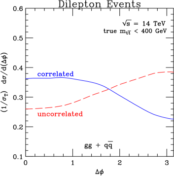
Figure 8: The differential distribution of $\Delta\phi$, $(1/\sigma_{T})~{}d\sigma/d(\Delta\phi)$. The solid curve is for the fully correlated case whereas the dashed curve assumes that the top quarks decay spherically in their respective rest frames. A cut restricting the invariant mass of the $t\bar{t}$ pairs to a maximum of 400 GeV has been applied to these distributions.

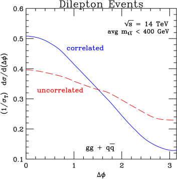
Figure 9: The differential distribution of $\Delta\phi$, $(1/\sigma_{T})~{}d\sigma/d(\Delta\phi)$. The solid curve is for the fully correlated case whereas the dashed curve assumes that the top quarks decay spherically in their respective rest frames. A cut restricting the average reconstructed invariant mass of the $t\bar{t}$ pairs to a maximum of 400 GeV has been applied to these distributions.

The simplest option one could imagine is to simply take the (naïve) unweighted average $\langle m_{t\bar{t}}\rangle$ of all of the real solutions returned by the neutrino reconstruction algorithm. In Fig. 9 we present the results of implementing just that option: the cut used to generate this figure requires that $\langle m_{t\bar{t}}\rangle$ be less than 400 GeV. With this cut approximately 5% of the total cross section for $t\bar{t}$ production survives at leading order. This is smaller than the fraction passing a 400 GeV cut on the true value of $m_{t\bar{t}}$ since only those events where all the spurious solutions are sufficiently small will survive. On the other hand, the sample passing this cut will contain a few events where the true value of $m_{t\bar{t}}$ is above 400 GeV, but, because the spurious solutions produced smaller values, the average was below 400 GeV. Turing to the $\Delta\phi$ distribution and comparing to the cut on the true value of $m_{t\bar{t}}$, one sees a rather large effect on the shape of the distributions. However, this effect (an enhancement near $\Delta\phi=0$ and a depletion near $\Delta\phi=\pi$) occurs for both the correlated and uncorrelated data sets. Thus the difference between the two distributions remains at roughly the 40% level. No effort has been to optimize this invariant mass cut. Perhaps there are other variables that will do better than unweighted average $\langle m_{t\bar{t}}\rangle$, or perhaps 400 GeV is not the optimal cut value. Nevertheless, what we have here is a proof-in-principle that these correlations can be measured in an experiment.

VI.2 ZMF $\cos\theta$ Distribution for Lepton-plus-jets Events

Turning to the lepton-plus-jets channel, we have found that the cosine of the opening angle between the charged lepton and the $d$-quark jet as viewed in the zero momentum frame (ZMF) is sensitive to the presence or absence of correlations between production and decay [see also the discussion near Eq. (53)]. For this type of event the kinematic constraints provide more equations than unknowns. Thus, the ZMF may be reconstructed without ambiguity more than 98% of the time by discarding those solutions which do not pass some rudimentary quality-control cuts: the neutrino energy ought to be positive in a correctly reconstructed event; futhermore, the neutrino and top quark mass-shell constraints ought to be satisfied to sufficient accuracy. Discarding the ${\sim}2\%$ of events that have more than one viable reconstruction of the ZMF is an acceptible option.

For the purposes of generating this distribution, we define the $d$-quark jet to be the jet which is spatially the closest to the $b$-tagged jet in the $W$ rest frame, as was used in Ref. mahlon and parke . This is equivalent to using the lowest energy jet in the top quark rest frame as advocated in Ref. Shelton:2008nq . Fig. 10 displays the results for this distribution using only those events that pass the cut $m_{t\bar{t}}<400$ GeV. For fully-correlated top decays this distribution is nearly flat, whereas for spherical decays there is a strong peaking near $\cos\theta=-1$. That is, because of the correlations between production and decay, the lepton and the $d$-jet tend to be significantly less back-to-back in the ZMF than if no such correlations were present. Approximately 9% of the total cross section for $t\bar{t}$ production survives this cut at leading order, even at reduced center-of-mass energy.

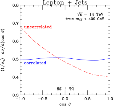
Figure 10: The differential distribution of $\cos\theta$, $(1/\sigma_{T})~{}d\sigma/d(\cos\theta)$, where $\theta$ is the ZMF angle between the charged lepton and the $d$-quark jet (defined to be the jet which is spatially the closest to the $b$-tagged jet in the $W$ rest frame; this is also the jet with the lowest energy in the top quark rest frame). The solid curve is for the fully correlated case whereas the dashed curve assumes that the top quarks decay spherically in their respective rest frames. A cut restricting the invariant mass of the $t\bar{t}$ pairs to a maximum of 400 GeV has been applied to these distributions.

VI.3 Varying the Energy of the LHC

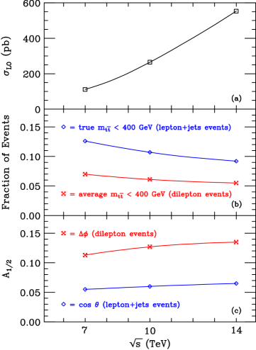
Figure 11: Effects of varying the machine center-of-mass energy $\sqrt{s}$. (a) Total leading order cross section for $pp\rightarrow t\bar{t}$. These values should be multiplied by the branching fraction to dileptons (4.6%) or lepton plus jets (29%), as appropriate. We include only the $e$ and $\mu$ channels. (b) Fraction of dilepton and lepton plus events with $m_{t\bar{t}}<400$ GeV. For dilepton events (crosses) we employ the unweighted average of the up to 8 solutions for the $t\bar{t}$ invariant mass. For lepton+jets events (diamonds) the true value of $m_{t\bar{t}}$ may be reconstructed and used in event selection. (c) Half of the area between the appropriate unit-normalized angular distributions for the fully correlated and spherical cases. For lepton+jets events (crosses), we use the distribtuion in $\cos\theta$, where $\theta$ is the angle between the charged lepton and the $d$-jet candidate in the zero momentum frame of the event. For dilepton events (diamonds), we use the azimuthal opening angle $\Delta\phi$ between the two charged leptons.

So far we have used 14 TeV for the energy of the LHC. However, it is now clear that the LHC will not reach this energy for a number of years so we have investigated what happens for a reduced center-of-mass energy in this section. The results we describe below are summarized in Fig. 11.

The primary result of a lower center-of-mass energy is a big reduction in the $t\bar{t}$ production cross section because of the reduced gluon luminosity. Panel (a) in Fig. 11 tracks the leading order cross section from 7 to 14 TeV center-of-mass energy. We see that a factor of 2 reduction in $\sqrt{s}$ produces a reduction of about a factor of 5 in the $t\bar{t}$ production cross section. Panel (b) illustrates the fact that the fraction of dilepton and lepton plus jet events surviving the $m_{t\bar{t}}$ or $\langle m_{t\bar{t}}\rangle$ cut we advocate does not change very much as $\sqrt{s}$ is varied between 7 and 14 TeV. Finally, in panel (c) of each figure we compare the quantity ${\cal A}_{1/2}$, which is defined as half of the area between the correlated and uncorrelated predictions for the unit-normalized angular distributions. This quantity ranges from 0 in the case where the distribution is completely independent of whether or not correlations are present up to 1 in the case where the two distributions (correlated decays or spherical decays) do not overlap at all. In both channels, there is relatively little dependence on $\sqrt{s}$ for this measure of the difference between the correlated and spherical cases. Thus, the biggest issue related to the observation of these spin correlations at the LHC running at reduced energy comes from the greatly diminished cross section: the correlations themselves remain at roughly the same level. Fortunately, even a reduction of the number number of $t\bar{t}$ pairs estimated in the introduction by a factor of 5 leaves ample statistics to hope for at least a preliminary observation of these spin correlation effects, even at reduced center-of-mass energy.

VI.4 NLO Effects

Higher-order QCD effects enhance the total cross section especially near threshold. However, previous studies on $e^{+}e^{-}\rightarrow t\bar{t}$ demonstrate that such corrections to the spin correlations are small, see Ref. Kodaira:1998gt . One can understand this physically since the emission of soft gluons from a top quark cannot flip the spin of the top quark. We have done a preliminary study of the NLO effects using both MCFM, MCFM and MC@NLO, Frixione:2007zp , incorporating a cut which restricts the invariant mass of the $t\bar{t}$ pair to be less than 400 GeV. Both these Monte Carlos show that the tree-level effects discussed earlier in this paper are also present at NLO. We need not check the Monte Carlo of Ref. Melnikov:2009dn since it agrees with the other two Monte Carlos for the correlated decays. A detailed study at NLO where the invariant mass of the $t\bar{t}$ pair is reconstructed from the decay products is beyond the scope of this work. A NLO Monte Carlo with a switch that allows the user to toggle between fully correlated top quark decays and spherical decays of the tops would be very useful for such a study. However, no such Monte Carlo exists at present.

VII Summary and Conclusions

In this paper we have shown how to observe spin correlations in top quark pair production at the LHC. To our surprise, the observation of these correlations is easier at the LHC than at the Tevatron. The reason for this is that at the LHC the dominant production mechanism for top quark pairs is gluon-gluon fusion, which at low $\hat{s}$ is dominated by the fusion of like helicity pair gluons. The fusion of like helicity gluons produces top quark pairs in a LL or RR helicity configuration. When such top quarks decay, they produce charged leptons which possess very strong azimuthal correlations. These correlations can be easily seen in the laboratory frame once a cut on the invariant mass of the top quark pair is made. There is not need to reconstruct the top quark rest frame as is required to see the correlations of top quark pairs at the Tevatron. The analysis has been extended to the lepton plus jets channel by “identifying” which jet is the $d$-quark jet from the $W$-boson decay on a statistical basis. Apart from the reduction of the total cross section, the size of these spin correlations is approximately independent of the energy of the LHC in the 7 to 14 TeV range. Thus, we expect that these effects could be observed in early running of the LHC.

Appendix A Universal Properties of the Spin Amplitudes

In this Appendix we demonstrate the properties of the spin amplitudes and their relationship to the Wigner $d$-functions and the helicity amplitudes. Of particular importance is the fact that spin amplitudes at either end of the spin chain contain all the information necessary to obtain all the other spin amplitudes by simple algebraic manipulations. This fact was used extensively earlier in this paper.

A.1 Wigner $d$-functions and connection to the spin amplitudes

The amplitude for production of a single massive particle with spin $j$ and spin-projection $m$ in the generalized spin basis described in Sect. II.1 and illustrated in Fig. 1 may be written as a linear superposition of the matrix elements of the rotation operator Jacob+Wick :

$${\cal A}_{j,m}(\xi) \equiv \langle\overrightarrow{x}|j\enspace m\rangle_{\xi}$$ (54)

$$= \sum_{m^{\prime}}d^{j}_{m,m^{\prime}}(-\xi)H_{m^{\prime}}.$$ (55)

The $d^{j}_{m,m^{\prime}}$ appearing in Eq. (55) are the Wigner $d$-functions, chosen to conform to the conventions of Rose Rose . In particular, we write $-\xi$ since our angle $\xi$ is measured in the clockwise direction whereas the angle $\beta$ in Ref. Rose is counterclockwise. Since

$$d_{m,m^{\prime}}^{j}(0)=\delta_{m,m^{\prime}},$$ (56)

we see that

$$H_{m}={\cal A}_{j,m}(0).$$ (57)

That is, the coefficients $H_{m}$ are the conventional helicity amplitudes for the process with a particular choice of relative phases.

Similarly, the production of a pair of massive particles (spins $j_{1}$ and $j_{2}$, spin projections $m_{1}$ and $m_{2}$ along independent spin axes oriented at the clockwise angles $\xi$ and $\xi^{\prime}$ with respect to the recoil direction in the scattering plane) may be decomposed as

$${\cal A}_{j_{{}_{1}},m_{{}_{1}},j_{{}_{2}},m_{{}_{2}}}(\xi,\xi^{\prime})=\sum_{m}\sum_{m^{\prime}}d^{j_{{}_{1}}}_{m_{{}_{1}},m}(-\xi)d^{j_{{}_{2}}}_{m_{{}_{2}},m^{\prime}}(-\xi^{\prime})H_{m,m^{\prime}}.$$ (58)

The extension to more than two particles in the final state or to spin axes which point out of the production plane, involving the introduction of the Wigner $D$-functions in place of the (simpler) $d$-functions, is straightforward, but beyond the scope of this appendix.

A.2 $\xi\rightarrow\xi\pm\pi$ rule

Intuitively, we expect that the probability for producing spin projection $+m$ along some axis ought to be equal to that for producing spin projection $-m$ along minus that axis:

$$|{\cal A}_{j,m}(\xi\pm\pi)|=|{\cal A}_{j,-m}(\xi)|.$$ (59)

That is, flipping the $z$ component of the spin and rotation by $\pm\pi$ give the same results up to a phase. This feature of the spin amplitudes is a consequence of the properties of the Wigner $d$-functions appearing in Eqs. (55) and (58).

A.3 Differential relations among the spin amplitudes

Consider a state with total spin $j$ and projection $j_{z}=m$ in the general spin basis illustrated in Fig. 1. Applying the rotation operator converts this to a state where the spin axis is at $\xi+\Delta\xi$ instead Jacob+Wick :

$${\cal A}_{j,m}(\xi+\Delta\xi)=e^{i\Delta\xi J_{y}}{\cal A}_{j,m}(\xi).$$ (60)

In the limit $\Delta\xi\rightarrow 0$ Eq. (60) may be rewritten as

$${{\partial}\over{\partial\xi}}{\cal A}_{j,m}(\xi)={1\over 2}(J_{+}-J_{-}){\cal A}_{j,m}(\xi).$$ (61)

In this expression, we have replaced $J_{y}$ by the appropriate linear combination of raising and lowering operators. Thus

$${{\partial}\over{\partial\xi}}{\cal A}_{j,m}(\xi) = {1\over 2}\sqrt{j(j+1)-m(m+1)}\thinspace{\cal A}_{j,m+1}(\xi)$$ (62)

$$- {1\over 2}\sqrt{j(j+1)-m(m-1)}\thinspace{\cal A}_{j,m-1}(\xi)$$ (63)

A.4 Starting at top or bottom of spin chain

It is useful to record the explicit results of applying Eq. (63) to the ends of the spin chain:

$${\cal A}_{j,\pm(j-1)}(\xi)=\mp\sqrt{2\over{j}}\thinspace{{\partial}\over{\partial\xi}}{\cal A}_{j,\pm j}(\xi).$$ (64)

A second differentiation allows us to conclude that

$${\cal A}_{j,\pm(j-2)}(\xi)={{{1}\over{\sqrt{j(2j{-}1)}}}\Biggl{[}j+2{{\partial^{2}}\over{\partial\xi^{2}}}}\Biggr{]}\thinspace{\cal A}_{j,\pm j}(\xi).$$ (65)

This process could be repeated as many times as required. However, when used in conjunction with the $\xi\rightarrow\xi\pm\pi$ rule of Eq. (59), Eqs. (64) and (65) allow the calculation of all of the amplitudes in the spin chain for spins up to and including $5\over 2$, starting from either end of the chain ($m=\pm j$). The relative simplicity of the operations involved in these relations makes for a substantial computational savings over the calculation of the complete set of amplitudes by direct means. Of course, once you have all the spin amplitudes then the helicity amplitudes can be easily obtained, including relative phases, by setting $\xi=0$.

Thus, the spin amplitudes at the top and bottom of the spin chain contain all the information about a given process and all other spin amplitudes and helicity amplitudes can be derived from them. This special property of these spin amplitudes is simply reflected in the Wigner $d$-functions, $d^{j}_{j,m}$ for $m=\{-j,\cdots,j\}$, which form a set of (2j+1) linearly independent functions edmonds .

A.5 Examples:

An explicit illustration of the relationships contained in Eqs. (64) and (65) is provided by the $gg\rightarrow t\bar{t}$ process considered in this paper. After setting $\xi^{\prime}=\xi$ (back-to-back spin axes in the ZMF), we can organize the amplitudes according to the total spin in the final state. In doing this we need to keep in mind that for this choice of spin axes, unlike spin $t\bar{t}$ pairs have spins that point in the same spatial direction. Thus

$$|{\cal A}_{1,1}(\xi)|=|{\cal A}(gg\rightarrow t_{\uparrow}\bar{t}_{\downarrow})|$$ (66)

and

$$|{\cal A}_{1,-1}(\xi)|=|{\cal A}(gg\rightarrow t_{\downarrow}\bar{t}_{\uparrow})|.$$ (67)

The $\xi$-dependent linear combination of the ${\uparrow}{\uparrow}$ and ${\downarrow}{\downarrow}$ amplitudes must be ${\cal A}_{1,0}$; the orthogonal ($\xi$-independent) combination is ${\cal A}_{0,0}$:

$$|{\cal A}_{1,0}(\xi)|={{1}\over\sqrt{2}}|{\cal A}(gg\rightarrow t_{\uparrow}\bar{t}_{\uparrow})+{\cal A}(gg\rightarrow t_{\downarrow}\bar{t}_{\downarrow})|,$$ (68)

$$|{\cal A}_{0,0}(\xi)|={{1}\over\sqrt{2}}|{\cal A}(gg\rightarrow t_{\uparrow}\bar{t}_{\uparrow})-{\cal A}(gg\rightarrow t_{\downarrow}\bar{t}_{\downarrow})|.$$ (69)

For like-helicity gluons Eqs. (31) and (32) lead to

$$|{\cal A}_{1,1}(\xi)| \sim \gamma^{-1}|\beta s_{\xi}|$$ (70)

$$|{\cal A}_{1,0}(\xi)| \sim \sqrt{2}\gamma^{-1}|\beta c_{\xi}|\qquad\hbox{and}\qquad|{\cal A}_{0,0}(\xi)|\sim\sqrt{2}\gamma^{-1}.$$ (71)

$$|{\cal A}_{1,-1}(\xi)| \sim \gamma^{-1}|\beta s_{\xi}|$$ (72)

The three $j=1$ amplitudes in (72) satisfy

$$|{\cal A}_{1,0}(\xi)|=\Bigl{|}\sqrt{2}{\partial\over{\partial\xi}}{\cal A}_{1,1}(\xi)\Bigr{|}$$ (73)

and

$$|{\cal A}_{1,-1}(\xi)|=\Biggl{|}\Bigl{\{}1+2{{\partial^{2}}\over{\partial\xi^{2}}}\Bigr{\}}{\cal A}_{1,1}(\xi)\Biggr{|}$$ (74)

as implied by Eqs. (64) and (65).

A different realization of these relationships is provided by the unlike-helicity gluons for which Eqs. (22) and (23) lead to

$$|{\cal A}_{1,1}(\xi)| \sim \beta s_{\theta}(1+c_{\theta}c_{\xi}+\gamma^{-1}s_{\theta}s_{\xi})$$ (75)

$$|{\cal A}_{1,0}(\xi)| \sim \sqrt{2}\beta s_{\theta}|c_{\theta}s_{\xi}-\gamma^{-1}s_{\theta}c_{\xi}|\qquad\hbox{and}\qquad|{\cal A}_{0,0}(\xi)|=0.$$ (76)

$$|{\cal A}_{1,-1}(\xi)| \sim \beta s_{\theta}(1-c_{\theta}c_{\xi}-\gamma^{-1}s_{\theta}s_{\xi})$$ (77)

This is identical (up to overall factors) to what happens for the processes $q\bar{q}\rightarrow t\bar{t}$ and similar to what happens for $e^{+}e^{-}\rightarrow t\bar{t}$ Parke:1996pr . The spin amplitudes for $e^{+}e^{-}\rightarrow Zh$ ref:deconstruction ; ZHZA also satisfy Eqs. (73) and (74).

Finally, we have verified that the processes $e^{+}e^{-}\rightarrow W^{+}W^{-}$ and $ZZ$ provide examples of the $j=2$ versions of Eqs. (64) and (65). Indeed, the derivative relations between the spin amplitudes for these processes noted in Ref. ref:deconstruction are a direct consequence of Eq. (64).

Appendix B The process $q\bar{q}\rightarrow t\bar{t}$

For completeness we give here the matrix element squared for $q\bar{q}\rightarrow t\bar{t}$ with the subsequent decay of the top quarks. Starting from Eqn. (12) and using the substitutions given in Eq. (49), it is easy to add the decays of the on-mass-shell top quarks ($t\rightarrow b+\bar{e}+\nu$ and $\bar{t}\rightarrow\bar{b}+\mu+\bar{\nu}$). Thus, the total matrix element squared for top quark production and decay via quark-antiquark annihilation, summed over the colors of the incoming and outgoing quarks, is given by

$$|{\cal A}|^{2}_{RL}+|{\cal A}|^{2}_{LR} = {\cal K}_{q\bar{q}}\Biggl{\{}2(t\cdot\bar{e})(\bar{t}\cdot\mu)\Bigr{[}(q\cdot t)^{2}+(\bar{q}\cdot t)^{2}\Bigl{]}$$

$$-m_{t}^{2}\Bigl{[}(q\cdot\bar{q})\Bigl{(}(t\cdot\bar{e})(t\cdot\mu)+(\bar{t}\cdot\bar{e})(\bar{t}\cdot\mu)-m_{t}^{2}(\bar{e}\cdot\mu)\Bigr{)}$$

$$\qquad-2\Bigl{(}(q\cdot t)(q\cdot\mu)(\bar{q}\cdot\bar{e})+(\bar{q}\cdot t)(q\cdot\bar{e})(\bar{q}\cdot\mu)-(q\cdot t)(\bar{q}\cdot t)(\bar{e}\cdot\mu)\Bigr{)}\Bigr{]}\Biggr{\}}.$$

This has the same functional form as the part of Eqn. (50) in the second set of curly brackets. The overall factor ${\cal K}_{q\bar{q}}$ is given by

$${\cal K}_{q\bar{q}}={{2^{6}g_{s}^{4}}\over{(q\cdot\bar{q})^{2}}}{{g_{w}^{8}}\over{(m_{t}\Gamma_{t})^{4}}}{{b\cdot\nu}\over{(2\bar{e}\cdot\nu-m^{2}_{w})^{2}+(m_{w}\Gamma_{w})^{2}}}{{\bar{b}\cdot\bar{\nu}}\over{(2\mu\cdot\bar{\nu}-m^{2}_{w})^{2}+(m_{w}\Gamma_{w})^{2}}}.$$ (79)

Eqs. (LABEL:eqn:qqbar-full) and (79) are the Lorentz-invariant equivalents of Eqs. (4) and (5) of Ref. Mahlon:1997uc .

References

- (1) See talk by Florencia Canelli at Lepton Photon 2009, http://lp09.desy.de/
- (2) G. Mahlon and S. J. Parke, Phys. Rev. D53, 4886 (1996) [arXiv:hep-ph/9512264].
- (3) T. Stelzer and S. Willenbrock, Phys. Lett. B 374, 169 (1996) [arXiv:hep-ph/9512292].
- (4) A. Brandenburg, Phys. Lett. B 388, 626 (1996) [arXiv:hep-ph/9603333].
- (5) S. J. Parke and Y. Shadmi, Phys. Lett. B 387, 199 (1996) [arXiv:hep-ph/9606419].
- (6) G. Mahlon and S. J. Parke, Phys. Lett. B 411, 173 (1997) [arXiv:hep-ph/9706304].
- (7) W. Bernreuther, A. Brandenburg and Z. G. Si, Phys. Lett. B 483, 99 (2000) [arXiv:hep-ph/0004184].
- (8) W. Bernreuther, A. Brandenburg, Z. G. Si and P. Uwer, Phys. Lett. B 509, 53 (2001) [arXiv:hep-ph/0104096].
- (9) W. Bernreuther, A. Brandenburg, Z. G. Si and P. Uwer, Phys. Rev. Lett. 87, 242002 (2001) [arXiv:hep-ph/0107086].
- (10) W. Bernreuther, A. Brandenburg, Z. G. Si and P. Uwer, Nucl. Phys. B 690, 81 (2004) [arXiv:hep-ph/0403035].
- (11) M. L. Mangano and S. J. Parke, Phys. Rept. 200, 301 (1991) [arXiv:hep-th/0509223].
- (12) R. Kleiss and W. J. Stirling, Nucl. Phys. B 262, 235 (1985).
- (13) M. Hori, Y. Kiyo and T. Nasuno, Phys. Rev. D58, 014005 (1998) [arXiv:hep-ph/9712379].
- (14) P. Uwer, Phys. Lett. B 609, 271 (2005) [arXiv:hep-ph/0412097].
- (15) J. Shelton, Phys. Rev. D 79, 014032 (2009) [arXiv:0811.0569 [hep-ph]].
- (16) J. Kodaira, T. Nasuno and S. J. Parke, Phys. Rev. D 59, 014023 (1999) [arXiv:hep-ph/9807209].
- (17) R. K. Ellis and J. M. Campbell provide us with a special version of MCFM which included all spin correlations for production at NLO.
- (18) S. Frixione, E. Laenen, P. Motylinski and B. R. Webber, JHEP 0704, 081 (2007) [arXiv:hep-ph/0702198].
- (19) K. Melnikov and M. Schulze, JHEP 0908, 049 (2009) [arXiv:0907.3090 [hep-ph]].
- (20) M. Jacob and G. C. Wick, Ann. Phys. 7, 404 (1959).
- (21) M. E. Rose, Elementary Theory of Angular Momentum, (John Wiley & Sons, Inc., New York, 1957).
- (22) A. R. Edmonds, Angular Momentum in Quantum Mechanics, (Princeton University Press, Princeton, 1957), page 59.
- (23) G. Mahlon and S. J. Parke, Phys. Rev. D58, 054015 (1998) [arXiv:hep-ph/9803410].
- (24) G. Mahlon and S. Parke, Phys. Rev. D74, 073001 (2006) [arXiv:hep-ph/0606052].