High-Order Conservative Finite Difference GLM-MHD Schemes for Cell-Centered MHD
Abstract
We present and compare third- as well as fifth-order accurate finite difference schemes for the numerical solution of the compressible ideal MHD equations in multiple spatial dimensions. The selected methods lean on four different reconstruction techniques based on recently improved versions of the weighted essentially non-oscillatory (WENO) schemes, monotonicity preserving (MP) schemes as well as slope-limited polynomial reconstruction. The proposed numerical methods are highly accurate in smooth regions of the flow, avoid loss of accuracy in proximity of smooth extrema and provide sharp non-oscillatory transitions at discontinuities.
We suggest a numerical formulation based on a cell-centered approach where all of the primary flow variables are discretized at the zone center. The divergence-free condition is enforced by augmenting the MHD equations with a generalized Lagrange multiplier yielding a mixed hyperbolic/parabolic correction, as in Dedner et al. (J. Comput. Phys. 175 (2002) 645-673). The resulting family of schemes is robust, cost-effective and straightforward to implement. Compared to previous existing approaches, it completely avoids the CPU intensive workload associated with an elliptic divergence cleaning step and the additional complexities required by staggered mesh algorithms.
Extensive numerical testing demonstrate the robustness and reliability of the proposed framework for computations involving both smooth and discontinuous features.
keywords:
Magnetohydrodynamics , Compressible Flow , Higher-order methods , WENO schemes , Monotonicity Preserving , Cell-centered methods1 Introduction
The development of high-order schemes has been receiving an increasing amount of attention from practitioners in the fields of fluid dynamics and, only more recently, magnetohydrodynamics (MHD). This interest is driven by a variety of reasons, such as the possibility of obtaining highly accurate solutions with reduced computational effort as well as the need to narrow the gap between the smallest resolved features and the dissipative scales. Although several successful strategies have been developed in the context of the Euler equations of gasdynamics, only few of them have been extended to MHD. In the present context, we focus our attention on high-order finite difference schemes for the solution of the compressible MHD equations in multiple spatial dimensions,
| (1) |
where , , , and are the fluid density, velocity vector, magnetic induction, energy and gas pressure, respectively. The system of equations (1) is complemented by the divergence-free constraint of the magnetic field,
| (2) |
and by an equation of state relating energy and pressures. For the present work we assume an ideal gas law
| (3) |
where is the ratio of specific heats.
Traditional second-order schemes have been largely employed for the solution of Eq. (1) using either finite volume (FV, e.g., [54, 44, 11, 23, 2, 19, 23, 40, 3]) or finite difference (FD, e.g., [5, 35, 13, 51, 22, 1, 32]) methods. At the second-order level, the two approaches are essentially equivalent and popular schemes have been built on Godunov-type discretizations based on the Total Variation Diminishing (TVD, [25]) property making use of slope-limited reconstructions. In spite of the excellent results produced in proximity of discontinuous waves where sharp non-oscillatory transitions can be obtained, TVD schemes still suffer from excessive unwanted numerical dissipation in regions of smooth flow. This deficiency owes to the inherent behavior of TVD methods that reduces the order of accuracy to first-order near local extrema (clipping) and smear linearly degenerate fields (such as contact waves) much more than shocks. Furthermore, discretization errors are mainly responsible for the loss of accuracy.
Efforts to relax the TVD condition and overcome these limitations have been spent over the last decades towards the development of highly accurate schemes that retain the robustness common to second-order Godunov-type methods. The original piecewise parabolic method (PPM) method by [14], for example, provides fourth-order accurate interface values in smooth regions (in 1D) and has been extended to MHD by [17, 18] and, more recently by [27, 28]. PPM, however, still degenerates to first-order at smooth extrema and attempts to solve the problem have been recently presented in [15] and [45].
Based on a different approach, weighted essentially non-oscillatory (WENO, [47]) schemes have improved on their ENO predecessor (originally proposed by Harten et al. [26]) and are now considered a powerful and effective tool for solving hyperbolic partial differential equations. WENO methods provide highly accurate solutions in regions of smooth flow and non-oscillatory transitions in presence of discontinuous waves by combining different interpolation stencils of order into a weighted average of order . The nonlinear weights are adjusted by the local smoothness of the solution so that essentially zero weights are given to non smooth stencils while optimal weights are prescribed in smooth regions. WENO scheme have been formulated in the context of MHD using both FD [30, 4] and FV formulations, [50, 5, 21, 6, 7]. Third- and fifth-order WENO schemes have been recently improved in terms of reduced dissipation, better resolution properties and faster convergence rates (see [53] and [9]) and will be considered here.
An alternative strategy is followed by the Monotonicity Preserving (MP) family of schemes by Suresh & Huynh [48] who proposed to carry the reconstruction step by first computing an accurate and stable interface value and then by imposing monotonicity- and accuracy-preserving constraints to limit the original value. MP schemes have been successfully merged with WENO methods by [4] and employed in the context of relativistic MHD by [16].
Finally, a reconstruction procedure that avoids the clipping phenomenon has been recently discussed by Čada & Torrilhon [10] who devised a new class of nonlinear limiter functions based upon a non-polynomial reconstruction showing good shape-preserving properties.
It is important to point out that, for spatial accuracy higher than two, multidimensional FV schemes become notoriously more elaborate than their FD counterparts, since point values can no longer be interchanged with volume averages. As a result, FV schemes generally require fully multidimensional reconstructions and the solution of several Riemann problems at a zone face providing the necessary number of quadrature points required by the desired level of accuracy, see, for instance, [12, 49, 5]. However, FV algorithms do have the adventage that they are better suited to non-uniform grids and adaptive mesh hierarchies. High-order FV schemes have been recently ameliorated in the work of [21, 6, 7] using either ADER-WENO schemes or least-squares polynomial reconstruction.
Conversely, multidimensional FD schemes evolve the point values of the conserved quantities and considerably ease up the coding efforts by restricting the computations of flux derivatives to one dimensional stencils. In this perspective, we present a new class of FD numerical schemes adopting a point-wise, cell-centered formulation of all of the flow quantities, including magnetic fields. The proposed schemes have order of accuracy three and five and their performance is compared through extensive testing on two and three-dimensional problems. Selected third-order accurate schemes are i) an improved version of the classical third-order WENO scheme of [29] based on new weight functions designed to improve accuracy near critical points [53] and ii) the recently proposed non-polynomial reconstruction of [10]. Selected fifth-order schemes include i) the WENO-Z scheme of [9] and ii) the monotonicity preserving scheme of [48] based on a fifth-order accurate interface value (MP5 henceforth).
The solenoidal constraint of the magnetic field is controlled by extending the hyperbolic/parabolic divergence cleaning technique of Dedner et al. [20] to FD schemes. This avoids the computational cost associated with an elliptic cleaning step as in [30], and the scrupulous treatment of staggered fields demanded by constrained transport algorithms, e.g. [5, 35, 27, 7]. Furthermore, Mignone & Tzeferacos [39] have shown through extensive testing, for a class of second-order accurate schemes, that the GLM approach is robust and can achieve accuracy comparable to the constrained transport. The resulting class of schemes is explicit and fully conservative in mass, momentum, magnetic induction and energy. Besides the ease of implementation and efficiency issues, the benefits offered by a method where all of the primary flow variables are placed at the same spatial position ease the task to add more complex physics.
The comparison between the different methods of solution is conveniently handled using the PLUTO code for computational astrophysics [37].
The paper is structured as follows. In §2 we describe the GLM-MHD equations, while §3 shows the finite difference formulation and the selected reconstruction methods. In §4 we test and compare the different scheme performance on problems involving the propagation of both continuous and discontinuous features. Conclusions are drawn in §5.
2 The Constrained GLM-MHD Equations
We look at a conservative discretization of the MHD equations (1) where all fluid variables retain a cell-centered collocation and enforce the divergence-free condition through the hyperbolic/parabolic divergence cleaning technique of Dedner’s [20]. In this approach Gauss’s and Faraday’s laws of magnetism are modified by the introduction of a new scalar field function or generalized Lagrangian multiplier (GLM henceforth) . The resulting system of GLM-MHD equations then reads
| (4) |
with conservative state vector and fluxes defined by
| (5) |
where labels the different components while is the delta Kronecker symbol. Equations (4) are hyperbolic and fully conservative with the only exception of the unphysical scalar field which satisfies a non-homogeneous equation with a source term. In the GLM approach, divergence errors are propagated to the domain boundaries at finite speed and damped at a rate given by (see §2).
The eigenvalues of the MHD flux Jacobians are all real and coincide with the ordinary MHD waves plus two additional modes , for a total of characteristic waves. Restricting our attention to the direction, they are given by
| (6) |
where
| (7) |
are the fast magneto-sonic ( with the sign), slow magneto-sonic ( with the sign) and Alfvén velocities. The two additional modes are decoupled from the remaining ones and corresponds to linear waves carrying jumps in and . These waves are made to propagate at the maximum signal speed compatible with the time step, i.e.,
| (8) |
where are the fast magneto-sonic speeds in the three directions and the maximum is taken throughout the domain.
Owing to the decoupling, one can treat the linear system given by the longitudinal component of the field and separately from the other ordinary -wave MHD equations. As we shall see, this greatly simplifies the solution process and allows to use the standard characteristic decomposition of the MHD equations.
Following [39], we divide the solution process into an homogeneous step, where the GLM-MHD (4) are solved with , and a source step, where integration is done analytically:
| (9) |
where is the minimum grid size. Extensive numerical testing has shown that divergence errors are minimized when the parameter lies in the range depending on the particular problem, although in presence of smooth flows this choice seems to be less sensitive to the numerical value of .
3 Finite Difference schemes
We consider a conservative finite difference discretization of (4) where point-values rather than volume averages are evolved in time. A uniform Cartesian mesh is employed with cell sizes centered at , where label the computational zones in the three directions. For clarity of exposition, we disregard the integer subscripts when redundant but always keep the half increment index notation when referring to a cell boundary, e.g., .
Integration in time resorts to a semi-discrete formulation where, given a high-order numerical approximation to the derivatives appearing on the right hand side of Eq. (4), one is faced with the solution of the following initial value problem
| (10) |
with initial condition given by the point-wise values of . We choose the popular third-order Runge-Kutta scheme [46, 24] to advance the solution in time, for which one has
| (11) |
The choice of the time step is restricted by the Courant-Friedrichs-Levy (CFL) condition:
| (12) |
where is the CFL number. Since the time step is proportional to the mesh size, the overall accuracy of the scheme is restricted to third-order because of the time-stepping introduced in Eq. (11).
Our task is now to provide a stable and accurate non-oscillatory numerical approximation to . To this purpose, we begin by focusing our attention to the direction and set, for ease of notations, . We then let point values of the flux correspond to the volume averages of another function, say , and define
| (13) |
In this formalism, point values of the flux are identified as cell averages of and may be regarded as the primitive function of . Straightforward differentiation of Eq. (13) yields the conservative approximation
| (14) |
Stated in this form, the problem consists of finding a high-order approximation to the interface values of knowing the undivided differences of the primitive function , a procedure entirely analogous to that used in the context of finite volume methods such as PPM [14]. Thus one can set
| (15) |
where is a highly accurate reconstruction scheme providing a stable interface flux value from point-wise values and the index spans through the interpolation stencil.
The procedure can be repeated in an entirely similar way also for the and flux contributions and allows to write the operator in (10) as
| (16) |
This yields the fully unsplit approach considered in this paper. Alternatively, one could use a directionally split formalism to obtain the solution through a sequence of one dimensional problems separately corresponding to each term in equation (16).
In order to ensure robustness and to avoid the appearance of spurious oscillations, the reconstruction step is best carried with the help of local characteristic fields and by separately evaluating contributions coming from right- and left-going waves. To this end we first compute, using the simple arithmetic average , left and right eigenvectors and of the Jacobian matrix , for each characteristic field . We then obtain a projection of the positive and negative part of the flux using a simple Rusanov Lax-Friedrichs flux splitting:
| (17) |
where and are the point-wise values of the flux and conservative variables. For a typical one-point upwind-biased approximation of order , one has while mirrors left-going characteristic fields with respect to the interface . The coefficient represents the maximum absolute value of the -th characteristic speed throughout the domain.
The global Lax-Friedrichs flux splitting thus introduced is particularly diffusive and other forms of splitting are of course possible, e.g. [29, 4]. However, we have found that the level of extra numerical dissipation tend to become less important for higher-order scheme.
The interface flux is then written as a local expansion in the right-eigenvector space:
| (18) |
where the coefficients
| (19) |
are the reconstructed interface values of the local characteristic fields and can be any one of the procedures described in §3.2.
3.1 Modification for the Constrained GLM-MHD equations
The procedure illustrated so far is valid for an arbitrary system of hyperbolic conservation laws, provided and satisfy
| (20) |
i.e., they are left and right eigenvectors of the flux Jacobian, respectively. However, following [20], we wish to exploit the full characteristic decomposition of the usual MHD equations rather than resorting to a full diagonalization procedure. To this purpose, we take advantage of the fact that the longitudinal component of the field and the Lagrange multiplier satisfy
| (21) |
and are thus decoupled from the remaining seven MHD equations. Eq. (21) defines a constant coefficient linear hyperbolic system with left and right eigenvectors given, respectively, by the rows and columns of
| (22) |
associated with the eigenvalues and . The linear system (21) can be preliminary solved to find the values of and at a given interface. Indeed, by applying the projection (17) to the linear system (21) using Eq. (22), one obtains that the only non trivial characteristic fields are
| (23) |
Since the eigenvectors are constant in space, the local projection at are completely unnecessary and the computations in Eq. (23) can be carried out very efficiently throughout the grid. Once (23) have been reconstructed using Eq. (19) one defines
| (24) |
and proceed by solving the ordinary MHD equations using defined by (24) as a constant parameter.
3.2 Third and Fifth-order Accurate Reconstructions
We have shown in §3 that flux derivatives may be written in conservative form by applying any one-dimensional finite volume reconstruction to the point values of the flux . Among the variety of different strategies we investigate both third- and fifth-order accurate interpolation schemes making use of three- and five-point stencil, respectively:
- 1.
- 2.
- 3.
- 4.
Our choice is motivated by the sake of comparing well-known and recently presented state of the art algorithms that rely on heavy usage of conditional statements (LimO3 and MP5) or completely avoid them (WENO+3 and WENO-Z).
The proposed algorithms are applied to the left (-) and right (+) propagating characteristic fields defined by Eq. (17) to provide an accurate interface value, formally represented by Eq. (19). Thus, in our formulation, the total number of reconstruction is : two for the linear characteristic fields defined by Eq. (23) and for the left- and right-going wave families defined by Eq. (17) with .
In the following we will drop the index for the sake of exposition and shorten either one of (17) with . Undivided difference will be frequently used and denoted with
| (25) |
Occasionally, we will also make use of the and functions defined, respectively as
| (26) |
3.2.1 Third-Order Improved WENO (WENO+3)
In the classical third-order WENO scheme of [29], the interface value is reconstructed using the information available on a three-point local stencil . More specifically, a third-order accurate value is provided by a linear convex combination of second-order fluxes:
| (27) |
The weights for are defined by
| (28) |
where are optimal weights and the smoothness indicators give a measure of the regularity of the corresponding polynomial approximation.
The scheme has been recently improved in the work by Yamaleev & Carpenter, [53], where the introduction of an additional nonlinear artificial dissipation term was shown to make the scheme stable in the L2-energy norm for both continuous and discontinuous solutions. Yamaleev & Carpenter also derived new weight functions providing faster convergence and improved accuracy at critical points. The improved weights are still defined by Eq. (28) with replaced by
| (29) |
To avoid loss of accuracy at critical points, it was shown in [53] that has to satisfy .
Here adopt the conventional third-order scheme defined by Eq. (27)-(28) but with replaced by Eq. (29) and simply set . This improves the accuracy over the original order scheme of [29] in regions where the solution is smooth and provides essentially non-oscillatory solutions near strong discontinuities and unresolved features. The improved third-order WENO scheme just described will be referred to as WENO+3.
3.2.2 Third-Order Limited reconstruction (LimO3 )
Recently, Čada and Torrilhon [10] have proposed a new and efficient third-order limiter function in the context of finite volume schemes. Similarly to the -order WENO scheme described in §3.2.1, the new limiter employs a local three-point stencil to achieve piecewise-parabolic reconstruction for smooth data and preserves the accuracy at local extrema, thus avoiding the well known clipping of classical second-order TVD limiters. Interface values are reconstructed using a simple piecewise-linear max/min function acting as a logical switch depending on the left and right slope:
| (30) |
where is the slope ratio, is the building block giving polynomial quadratic reconstruction and is the third-order limiter
| (31) |
The function in Eq. (30) smoothly switches between limited and unlimited reconstructions based on a local indicator function properly introduced to avoid loss of accuracy at smooth extrema with one vanishing lateral derivative:
| (32) |
where . The function measures the curvature of non-monotone data inside a computational zone and the free-parameter is used to discriminate between smooth extrema and shallow gradients. Larger values of noticeably improve the reconstruction properties at the cost of introducing more local variation, see [10]. In the tests presented here we use .
3.2.3 Fifth-Order Improved WENO: WENO-Z
Borges et al. [9] presented an improved version of the classical fifth-order weighted essentially non-oscillatory (WENO) FD scheme of [29]. The new scheme, denoted with WENO-Z, has been shown to be less dissipative and provide better resolution at critical points at a very modest additional computational cost. We will employ such scheme here and, for the sake of completeness, report only the essential steps for its implementation (for a thorough discussion see the paper by [9]).
Following the general idea of WENO reconstruction, one considers the convex combination of different third-order accurate interface values built on the three possible sub-stencils of :
| (33) |
The weights for are defined by
| (34) |
where are the optimal weights giving a fifth-order accurate approximation, is a small number preventing division by zero and the smoothness indicators give a measure of the regularity of the corresponding polynomial approximation:
| (35) |
While maintaining the essentially non-oscillatory behavior, the new formulation makes use of higher-order information about the regularity of the solution thus providing enhanced order of convergence at critical points as well as reduced dissipation at discontinuities.
3.2.4 Fifth-order Monotonicity Preserving (MP5)
The monotonicity preserving (MP) schemes of Suresh & Huynh [48] achieve high-order interface reconstruction by first providing an accurate polynomial interpolation and then by limiting the resulting value so as to preserve monotonicity near discontinuities and accuracy in smooth regions. The MP algorithm is better sought on stencils with five or more points in order to distinguish between local extrema and a genuine discontinuities. Here we employ the fifth-order accurate scheme based on the (unlimited) interface value given by
| (36) |
based on the five point values . Together with (36), we also define the monotonicity-preserving bound
| (37) |
resulting from the median between , and the left-sided extrapolated upper limit . The parameter controls the maximum steepness of the left sided slope and preserves monotonicity during a single Runge-Kutta stage (Eq. 11) provided the CFL number satisfies . In practice, setting still allows larger values of to be used. The interface value given by Eq. (36) is not altered when the data is sufficiently smooth or monotone that lies inside the interval defined by . Otherwise limiting takes place by bringing the original value back into a new interval specifically designed to preserve accuracy near smooth extrema and provide monotone profile close to discontinuous data. The final reconstruction can be written as
| (38) |
where
| (39) |
The bounds given by Eq. (39) provide accuracy-preserving constraints by allowing the original interface value to lie in a somewhat larger interval than or . This is accomplished by considering the intersection of the two extended intervals and that leave enough room to accommodate smooth extrema based on a measure of the local curvature defined by
| (40) |
where . Using Eq. (40), one defines the median and the large curvature values as
| (41) |
respectively. The curvature measure provided by (40) is somewhat heuristic and chosen to reduce the amount of room for local extrema to develop. The reconstruction illustrated preserves monotonicity and does not degenerate to first-order in proximity of smooth extrema.
4 Numerical Tests
In this section we present a series of test problems aimed at the verification of the FD methods previously described. The selected algorithms have been implemented in the PLUTO code for astrophysical gas-dynamics [37] in order to ease inter-scheme comparisons through a flexible common computational framework.
Unless otherwise stated, the specific heat ratio will be set to and the Courant number will be taken equal to , or for one, two and three dimensional computations, respectively. Errors for a generic flow quantity are computed using the discrete norm defined by
| (42) |
where the summation extends to all grid zones, and are the number of grid points in the three directions and is a reference solution. The divergence of magnetic field is quantified using Eq. (42) with computed as
| (43) |
where the interface values are obtained through Eq. (24).
4.1 Propagation of Circularly polarized Alfvén Waves
We start by considering a planar, circularly polarized Alfvén wave propagating along the direction. As the wave propagates, density and pressure stay constant whereas transverse vector components trace circles without changing their magnitude. Denoting with and the angular frequency and wavenumber, respectively, one has
| (44) |
where , is the corresponding phase velocity ( is the Alfvén speed) and is the wave amplitude. The plus or minus sign corresponds to right or left propagating waves, respectively. Here we consider a standing wave for which one has and further set , .
The one-dimensional solution given by (44) is first rotated by an angle around the axis and subsequently by an angle around the axis, as in [39]. The resulting transformation leaves scalar quantities invariant and produces vector rotations , where is either velocity or magnetic field and
| (45) |
are the rotation matrix and its inverse.
Note that the rotation can be equivalently specified by prescribing the orientation of the wave vector in a three-dimensional Cartesian frame through the angles and such that
| (46) |
such that . With these choices, in (44) becomes where .
Periodicity is guaranteed by setting, without loss of generality, and by choosing the computational domain , and . With these definitions the wave returns into the original position after one period
| (47) |
Different configurations can be specified in terms of the four parameters and (background pressure). One and two dimensional propagation are recovered by setting and , respectively.
4.1.1 One Dimensional Propagation
| One Dimension | Three Dimensions | ||||
|---|---|---|---|---|---|
| Method | |||||
| WENO+3 | 16 | 3.45E-03 | - | 2.54E-02 | - |
| 32 | 4.39E-04 | 2.97 | 3.68E-03 | 2.79 | |
| 64 | 5.52E-05 | 2.99 | 4.47E-04 | 3.04 | |
| 128 | 6.91E-06 | 3.00 | 5.51E-05 | 3.02 | |
| 256 | 8.64E-07 | 3.00 | 6.85E-06 | 3.01 | |
| LimO3 | 16 | 3.36E-03 | - | 2.82E-02 | - |
| 32 | 4.36E-04 | 2.95 | 3.76E-03 | 2.91 | |
| 64 | 5.53E-05 | 2.98 | 4.34E-04 | 3.11 | |
| 128 | 6.91E-06 | 3.00 | 5.46E-05 | 2.99 | |
| 256 | 8.65E-07 | 3.00 | 6.84E-06 | 3.00 | |
| WENO-Z | 16 | 7.50E-04 | - | 4.10E-03 | - |
| 32 | 2.40E-05 | 4.96 | 1.32E-04 | 4.96 | |
| 64 | 7.55E-07 | 4.99 | 3.89E-06 | 5.09 | |
| 128 | 2.36E-08 | 5.00 | 1.20E-07 | 5.02 | |
| 256 | 7.37E-10 | 5.00 | 3.74E-09 | 5.00 | |
| MP5 | 16 | 7.38E-04 | - | 3.41E-03 | - |
| 32 | 2.40E-05 | 4.94 | 1.19E-04 | 4.84 | |
| 64 | 7.55E-07 | 4.99 | 3.81E-06 | 4.97 | |
| 128 | 2.36E-08 | 5.00 | 1.20E-07 | 4.99 | |
| 256 | 7.37E-10 | 5.00 | 3.74E-09 | 5.00 | |
As a first test, we consider one-dimensional propagating waves on the segment using grid points with . We set the background pressure to be and the wave amplitude . The GLM correction is not necessary and has turned off for one dimensional propagation.
In order to investigate the convergence of solution, the integration time step is adjusted to
| (48) |
where is the nominal time increment at the minimum resolution , whereas is the spatial accuracy of the scheme. Errors (in norm) for the four selected schemes are plotted after one wave period in the left panel of Fig 1 and arranged, together with the corresponding order of convergence, in the third and fourth columns of Table 1. All schemes meet the expected order of accuracy (i.e. 3 for LimO3 and WENO+3, 5 for WENO-Z and MP5) with no significant differences. It is remarkable that, at the resolution of zones, the fifth-order schemes achieve essentially the same accuracy as the third-order schemes that make use of four times (i.e. ) as many points.
4.1.2 Three Dimensional Oblique Propagation
A three dimensional configuration is obtained by rotating the one-dimensional setup described in §4.1.1 by the angles so that in Eq. (45). The background pressure is and the wave has amplitude . The size of the computational box turns out to be , , and the number of grid points is set by , where changes as in §4.1.1. Integration lasts for one wave period, i.e., and the time step is determined by the same condition given by Eq. (48). Thus, apart from the different normalization, our setup is identical to that used in [28].
Errors are plotted at different resolutions in the right panel of Fig 1 and sorted in Table 1 for all schemes. On average, errors are larger than their one-dimensional counterparts but the overall behavior meets the expected order of accuracy with MP5 and LimO3 performing slightly better than WENO-Z and WENO+3, respectively. As for the 1D case, roughly of the resolution is required by a fifth-order scheme to match the accuracy of a third-order one.
Following [28], we construct in Fig 2 a scatter plot of the magnetic field component parallel to the axis of the original one dimensional frame. This is achieved by plotting, for every point in the computational domain, the component of as a function of the normal () coordinate of , where is the rotation matrix introduced in (45). The ability of the scheme to retain the planar symmetry during the computation is confirmed by the lack of scatter in the plots. The profiles at different resolutions verify the general trend established in Table 1 and deviations from the exact solution appear to be imperceptible for for the third-order schemes and already at for the fifth-order schemes.
Overally, the results obtained with third- and fifth-order accurate schemes outperform traditional TVD schemes, such as the CT-PPM algorithm of [28] yielding at most second-order accurate solutions. The CPU costs associated with WENO+3, LimO3 , WENO-Z and MP5 show, for this test problem, a relative scaling , respectively.
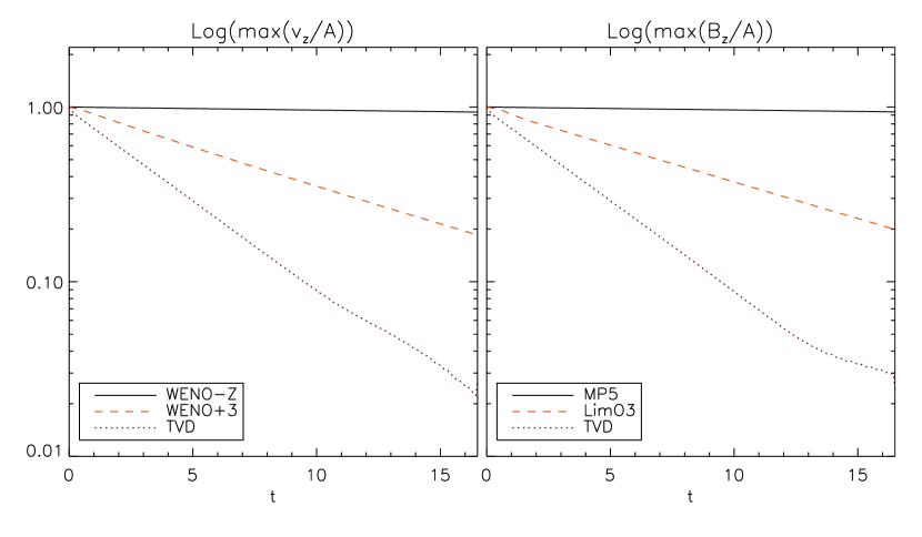
4.1.3 Numerical Dissipation and Long Term Decay in Two Dimensions
As already stated, circularly polarized Alfvén waves are an exact nonlinear solution of the MHD equations and measuring their decay provides a direct indication of the intrinsic numerical viscosity and resistivity possessed by the underlying algorithm, see [44, 5, 6]. This study is relevant, for example, in the field of MHD turbulence modeling where one should carefully control the amount of directionally-biased dissipation introduced by waves propagating inclined to the mesh. The error introduced during an oblique propagation is usually minimized at since contributions coming from different directions have comparable magnitude. On the contrary, waves propagating at smaller inclination angles make the problem more challenging.
Our setup builds on [5] although we adopt a slightly different, more severe, configuration. Using the notations introduced in §4.1, we set , , and prescribe the background pressure to be . The corresponding ratio of the plasma pressure to the (unperturbed) magnetic pressure is then given by , where is the wave propagation speed. The choice of the inclination angle determines the computational domain , as well as the wave period from Eq. (47). The final integration time is chosen by having the wave cross the domain times. This configuration results in a more arduous test than [5] where the wave period was longer and the integration was stopped after wave transits.
Fig 3 shows, at the resolution of mesh points, the maximum values of the vertical components of velocity (left panel) and magnetic field (right panel) as functions of time. By the end of the simulation, third-order schemes (dashed lines) show some degree of dissipation with the wave amplitude being reduced to per cent of its initial value. On the contrary, schemes of order five (solid lines in the figure) preserve the original shape more accurately and the amplitude retains per cent of its nominal value. These results are compared, for illustrative purposes, to a order TVD scheme using the Monotonized Central difference limiter (dotted lines), showing that the initial peak values have scaled down to per cent, thus showing a considerably larger level of numerical dissipation.
4.2 Shock tube problems
Shock tube problems are commonly used to test the ability of the scheme in describing both continuous and discontinuous flow features. In the following we consider two and three dimensional rotated configurations of standard one dimensional tubes. The default value for the parameter controlling monopole damping (see Eq. 9) is .
4.2.1 Two-Dimensional Shock tube
Following [30, 33], we consider a rotated version of the Brio-Wu test problem [8] with left and right states are given by
| (49) |
where is the vector of primitive variables. The subscript “1” gives the direction perpendicular to the initial surface of discontinuity whereas “2” corresponds to the transverse direction. Here is used and the evolution is interrupted at time , before the fast waves reach the borders.
In order to address the ability to preserve the initial planar symmetry we rotate the initial condition by the angle in a two dimensional plane with and using grid points, with . Vectors follow the same transformation given by Eq. (45) with . This is known to minimize errors of the longitudinal component of the magnetic field (see for example the discussions in [52, 27]). Boundary conditions respect the translational invariance specified by the rotation: for each flow quantity we prescribe where , with the plus (minus) sign for the leftmost and upper (rightmost and lower) boundary. Computations are stopped before the fast rarefaction waves reach the boundaries, at .
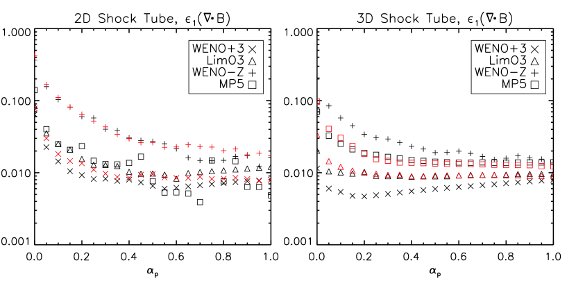
Fig 4 shows the primitive variable profiles for all schemes against a one-dimensional reference solution obtained on a base grid of zones with levels of refinement. Errors in norm, computed with respect to the same reference solution, are sorted in Table 2 for density and the normal component of magnetic field. The out-coming wave pattern is comprised, from left to right, of a fast rarefaction, a compound wave (an intermediate shock followed by a slow rarefaction), a contact discontinuity, a slow shock and a fast rarefaction wave. We see that all discontinuities are captured correctly and the overall behavior matches the reference solution very well. The normal component of magnetic field is best described with MP5 and does not show erroneous jumps. Indeed, the profiles are essentially constant with small amplitude oscillations showing a relative peak . Divergence errors, typically , remain bounded with resolution and tend to saturate when the damping parameter for both 2 and 3D calculations, see Fig 7. In this sense, our results favourably compare to those of [30, 33] and [21].
Fifth-order methods exhibit less dissipation across jumps, with fewer points in each discontinuous layer. Still, the accuracy gained from third to fifth-order accurate schemes (see Table 2) is only a factor since interpolation across discontinuities usually degenerates to lower-order to suppress spurious oscillations.
| Two Dimensions | Three Dimensions | |||||
|---|---|---|---|---|---|---|
| Method | ||||||
| WENO+3 | 4.11E-03 | 8.53E-05 | 7.19E-03 | 1.82E-03 | 4.41E-05 | 7.12E-03 |
| LimO3 | 3.61E-03 | 8.74E-05 | 1.08E-02 | 1.63E-03 | 4.07E-05 | 9.41E-03 |
| WENO-Z | 2.72E-03 | 7.90E-05 | 1.48E-02 | 1.29E-03 | 5.41E-05 | 1.59E-02 |
| MP5 | 2.31E-03 | 6.24E-05 | 7.60E-03 | 1.07E-03 | 2.22E-05 | 1.37E-02 |
4.2.2 Three-Dimensional Shock tube
The second Riemann problem was introduced by [43] and later considered by [44, 52, 4] and by [28, 39] in 3D. The primitive variables are initialized as
| (50) |
where . A reference solution at is obtained on the domain using grid points and levels of refinement. Our setup draws on the three dimensional version of [28] and [39] where the initial condition (50) is rotated using Eq. (45) by the angles and such that and (corresponding to ). With this choice the planar symmetry is respected by an integer shift of cells. The computational domain consists of zones and spans in the direction while . Computations stop at (note the misprint in [39]).
Fig 5 and 6 show primitive variable profiles obtained with third- and fifth-order schemes, respectively. The wave pattern consists of a contact discontinuity that separates two fast shocks, two slow shocks and a pair of rotational discontinuities. Table 2 confirms again that the gain from high-order methods is not particularly significant when the flow is discontinuous. Our results favorably compare with those of other investigators and no prominent over/under-shoots are observed. Moreover, the amount of oscillations in the normal component of the magnetic field is comparable to (or smaller than) those found in [28, 39] and divergence errors behave in a very similar way to the 2D case (see also the right panel in Fig 7).
The computational costs relative to that of WENO+3 () are found, for this problem, to be for LimO3 , WENO-Z and MP5, respectively.
4.3 Iso-density MHD Vortex advection
The following problem has been introduced in [5] and lately considered by [6, 7, 21]. The initial condition, satisfying the time-independent MHD equations, consists of a magnetized vortex structure in force equilibrium that propagates along the main diagonal of the computational box (a square in 2D and a cube in 3D). Here we set .
4.3.1 Two Dimensional Propagation
Following Dumbser et al. [21], we perform computations on the Cartesian box with an initial flow described by , , and . The constants and are chosen to be equal to while . The simulations are evolved for 10 time units with periodic boundary conditions, i.e. a single passage of the vortex through the domain. The parameter is chosen equal to for third-order schemes, effectively reproducing the configuration shown in [5, 7]. For WENO-Z and MP5, on the other hand, we choose in order to reduce the unwanted effects produced by the small jump in the magnetic field at the periodic boundaries, as argued in [21].
In order to compare our results to the findings of the latter study, we report, in Table 3, errors for measured both in and norms and the corresponding convergence rates. All schemes quickly converge to the asymptotic order of accuracy. Remarkably, errors obtained with the third-order schemes are identical and somewhat better than those of [7]. At the resolution of , fifth-order schemes yield errors times smaller than third-order ones at . A comparison between third- and fifth-order schemes from Fig 12 reveals that divergence errors rapidly decrease with resolution following a similar pattern. This eloquently advocates towards the use of higher-order schemes.
| Two Dimensions | Three Dimensions | ||||||||
|---|---|---|---|---|---|---|---|---|---|
| Method | |||||||||
| WENO+3 | 32 | 2.49E-03 | - | 1.94E-04 | - | 7.81E-04 | - | 1.74E-05 | - |
| 64 | 4.13E-04 | 2.6 | 1.73E-05 | 3.5 | 1.29E-04 | 2.6 | 1.12E-06 | 4.0 | |
| 128 | 5.72E-05 | 2.9 | 1.16E-06 | 3.9 | 1.82E-05 | 2.8 | 5.38E-08 | 4.4 | |
| 256 | 7.69E-06 | 2.9 | 7.24E-08 | 4.0 | - | - | - | - | |
| LimO3 | 32 | 2.49E-03 | - | 1.94E-04 | - | 7.81E-04 | - | 1.74E-05 | - |
| 64 | 4.13E-04 | 2.6 | 1.73E-05 | 3.5 | 1.29E-04 | 2.6 | 1.12E-06 | 4.0 | |
| 128 | 5.72E-05 | 2.9 | 1.16E-06 | 3.9 | 1.82E-05 | 2.8 | 5.38E-08 | 4.4 | |
| 256 | 7.69E-06 | 2.9 | 7.24E-08 | 4.0 | - | - | - | - | |
| WENO-Z | 32 | 8.17E-04 | - | 1.02E-04 | - | 1.63E-04 | - | 7.39E-06 | - |
| 64 | 5.10E-05 | 4.0 | 2.89E-06 | 5.1 | 1.07E-05 | 3.9 | 1.50E-07 | 5.6 | |
| 128 | 1.83E-06 | 4.8 | 5.23E-08 | 5.8 | 3.78E-07 | 4.8 | 1.87E-09 | 6.3 | |
| 256 | 5.94E-08 | 4.9 | 8.28E-10 | 6.0 | - | - | - | - | |
| MP5 | 32 | 9.57E-04 | - | 1.04E-04 | - | 1.96E-04 | - | 7.34E-06 | - |
| 64 | 5.16E-05 | 4.2 | 3.02E-06 | 5.1 | 1.07E-05 | 4.2 | 1.53E-07 | 5.6 | |
| 128 | 1.75E-06 | 4.9 | 5.15E-08 | 5.9 | 3.66E-07 | 4.9 | 1.85E-09 | 6.4 | |
| 256 | 5.69E-08 | 4.9 | 8.04E-10 | 6.0 | - | - | - | - | |
4.3.2 Three Dimensional Propagation
We propose a novel three dimensional extension of the vortex problem, consisting of similar initial conditions as the 2D case, albeit the radius now refers to the spherical one, . The perturbation of pressure is now given by
| (51) |
while we prescribe also a vertical velocity . The computational domain is the cube with periodic boundary conditions. The evolution stops after 10 time units.
The last four columns of Table 3 report the and norm errors of showing an excellent agreement with the analytical solution. Notice that the errors measured in norm are systematically smaller than errors and a comparison between similar configurations using different norms (as reported in [21]) may be deceitful. Keeping that in mind and given the somewhat diverse configurations, one can see that our results (in norm) are competitive with those of [21] at least at a qualitative level.
Divergence errors, shown in Fig 12, quickly decrease as the mesh thickens and fall below at the resolution of for the fifth-order schemes.
The computational cost is in accordance with previous tests, giving a ratio of for WENO+3, LimO3 , WENO-Z and MP5, respectively.
4.4 Advection of a magnetic field loop
We now consider the advection of a magnetic field loop. For sufficiently large plasma , specifying a thermal pressure dominance, the loop is transported as a passive scalar. The preservation of the initial circular shape tests the scheme’s dissipative properties and the correct discretization balance of multidimensional terms [27, 28, 32, 39].
4.4.1 Two Dimensional Propagation
Following [27, 22], the computational box is defined by and discretized on grid cells (). Density and pressure are initially constant and equal to . The velocity of the flow is given by with , and . The magnetic field is defined through its magnetic vector potential as
| (52) |
where , , , , and . The modification to the vector potential in the region (with respect to similar setups presented by other investigators) is done to remove the singularity in the loop’s center that can cause spurious oscillations and erroneous evaluations of the magnetic energy. The simulations are allowed to evolve until ensuring the crossing of the loop twice through the periodic boundaries.
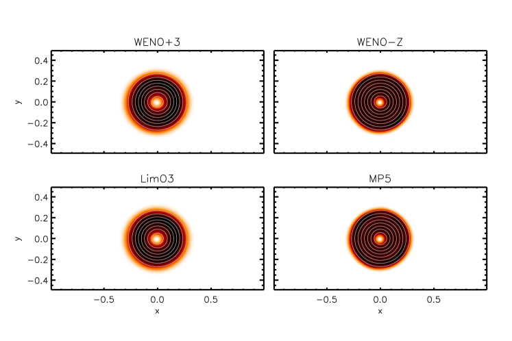
In Fig. 8 the magnetic energy density is displayed for the LimO3 , WENO+3, WENO-Z and MP5 schemes, along with iso-contours of the component of the magnetic vector potential. The initial circular shape is preserved well by all schemes. The third-order schemes are substantially more diffusive, as can be seen on the borders of the loop. This is confirmed by the time evolution of the magnetic energy density (normalized to its initial value), plotted in the left panel of Fig.9. The power law behaviour is similar for the schemes of the same order, with the MP5 method being the least diffusive. No pronounced difference is found between the LimO3 and WENO+3 schemes, for this particular problem.
The divergence of magnetic field measured in norm is shown in the left panel of Fig 11, as a function of . For the fifth-order schemes errors are minimized when whereas LimO3 and WENO+3 present smaller errors for .
4.4.2 Three Dimensional Propagation
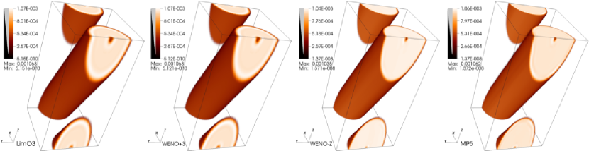
The three dimensional version of this problem is particularly challenging as the correct evolution depends on how accurately the condition is preserved and how the multidimensional MHD terms are balanced out. The computational domain , , is resolved onto zones. As for the two-dimensional case the vector potential is used to initialize the magnetic field, which is then rotated using the coordinate transformation given by Eq. (45) with and . Even though the loop is rotated only around one axis, the velocity profile makes the test intrinsically three-dimensional. Once again, pressure and density are taken uniform and equal to unity while boundary conditions are periodic in all directions.
The preservation of the loop’s shape can be seen in Fig. 10. All schemes preserve the shape, with LimO3 and WENO+3 being equally more diffusive (notice the thickness of the dark area at the loop’s borders, as well as the brighter ring just inside the loop). As for the 2D case, one can see that MP5 is the least diffusive in preserving the magnetic energy (right panel of Fig. 9), while the dissipation rates for LimO3 and WENO+3 practically coincide. Moreover, the three-dimensional norm error of (right panel of Fig 11) exhibits a behaviour similar to the two dimensional case. As before, the relative CPU scaling between WENO+3, LimO3 , WENO-Z and MP5 for this test problem is .
4.5 Orszag-Tang
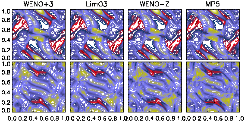
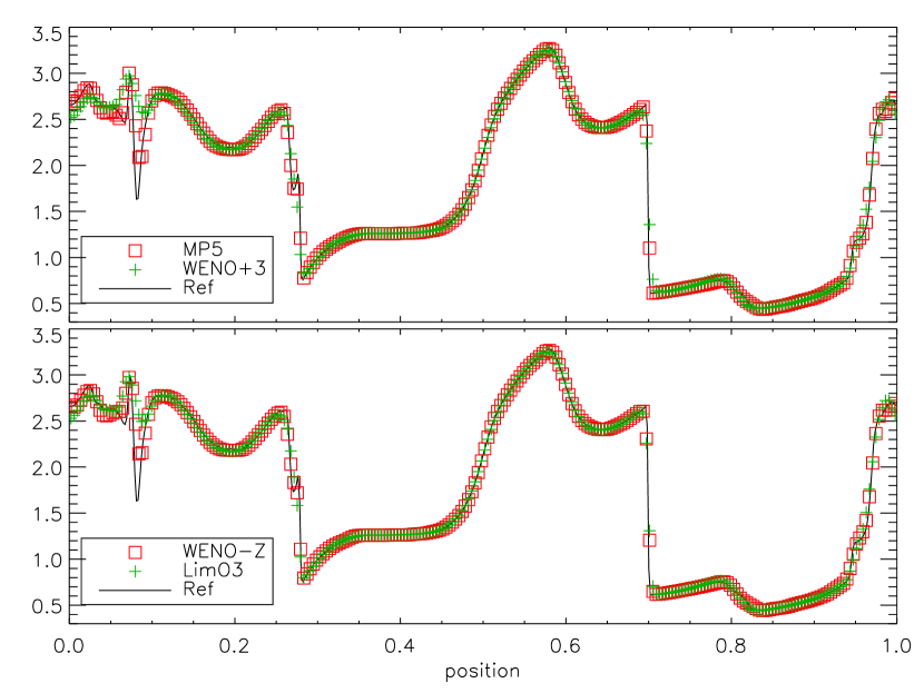
The Orszag-Tang vortex system describes a doubly periodic fluid configuration leading to two-dimensional supersonic MHD turbulence. The domain is initially filled with constant density and pressure respectively equal to and , while velocity and magnetic field are initialized to and , respectively. Although an analytical solution is not known, its simple and reproducible set of initial conditions has made it a widespread benchmark for inter-scheme comparison, see for example [52]. Density contour plots, as in [32] are shown in the top and bottom rows of Fig. 13 at and , respectively, using a resolution of points. The dynamics is regulated by multiple shock interactions leading to the formation of small scale vortices and density fluctuations. Our results at are in good agreement with previous investigations, e.g. [30, 52, 35, 42, 32], with WENO+3 and LimO3 showing increased numerical dissipation when compared to WENO-Z and MP5. This is further confirmed in Fig 15 where horizontal cuts at in the pressure distribution are plotted against a reference solution obtained with the second-order CT-CTU scheme of [27] on a finer mesh (), see also [30, 34, 42].
The most noticeable difference occurs at , when the fifth-order schemes (in particular, MP5) reveal the formation of a central magnetic island featuring a high density spot also recognizable in the results of [32] and in [2, 38] for the isothermal case. This structure is absent in the third-order schemes and may be induced by the decreased effective resistivity across the central current sheet, as discussed in [38].
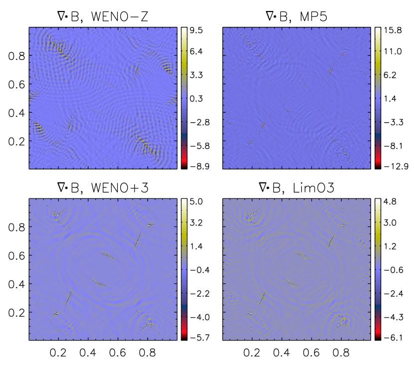
Divergence errors, shown in Fig 14 at , are comparable with those given by other investigators (e.g. [42, 33]) and reach their maximum magnitude in presence of discontinuous features.
The computational cost of LimO3 , WENO-Z and MP5 relative to that of WENO+3 () are found to be , in analogy with the previous results.
4.6 Kelvin-Helmholtz Unstable Flows
As a final example, we propose the nonlinear evolution of the Kelvin-Helmholtz instability in two dimensions. The base flow consists of a single shear layer with an initially uniform magnetic field lying in the plane at an angle with the direction of propagation:
| (53) |
where is the Mach number, is the steepness of the shear, is the Alfvén speed. Density and pressure are initially constant and equal to and . A single-mode perturbation with , is super-imposed as in [36]. Computations are carried out in a Cartesian box for time units on a mesh, where .
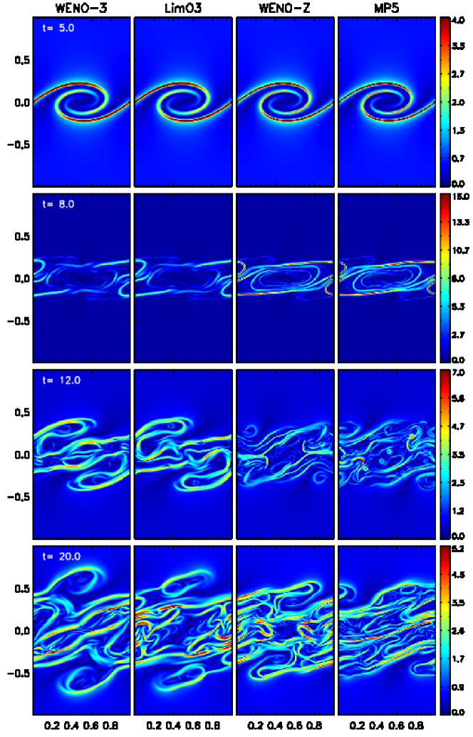
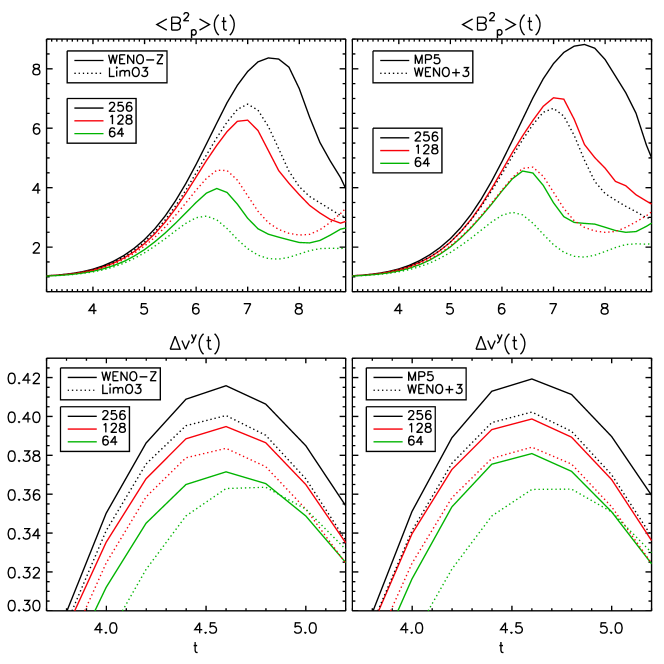
The evolutionary stages are shown in Fig 16, where we display color maps of the ratio at the largest resolution for WENO+3, LimO3 , WENO-Z and MP5. For the perturbation follows a linear growth phase during which magnetic field lines wound up through the formation of a typical cat’s eye vortex structure, [36, 31], see the top row in Fig 16. During this phase, magnetic field lines become distorted all the way down to the smaller diffusive scales and the resulting field amplification becomes larger for higher magnetic Reynolds numbers. As such, we observe in the top row of Fig 17 that the magnetic energy grows faster not only as the resolution is increased from to mesh points (green, red, black), but also when switching from a third-order to a fifth order scheme (solid vs. dotted lines). In particular, one can see that half of the grid resolution is needed by MP5 to match the results obtained with WENO+3. A somewhat lesser gain can be inferred by comparing WENO-Z and LimO3 . Similarly, the growth rate (computed as see bottom panel in Fig. 17), is closely related to the poloidal field amplification and evolves faster for smaller numerical resistivity and thus for finer grids and/or less dissipative schemes.
Field amplification is eventually prevented when by tearing mode instabilities leading to reconnection events capable of expelling magnetic flux from the vortex (second row in Fig. 16), [31]. Throughout the saturation phase (third and fourth row in Fig 16) the mixing layer enlarges and the field lines thicken into filamentary structures. During this phase one can clearly recognize that small scale structures are best spotted with the fifth-order methods while they appear to be more diffused with WENO+3 and LimO3 .
The CPU costs relative to that of WENO+3 () follow the ratios for LimO3 , WENO-Z and MP5, respectively, and confirm the same trend already established in previous tests.
5 Conclusions
We have presented a class of high-order finite difference schemes for the solution of the compressible ideal MHD equations in multiple spatial dimensions. The numerical framework adopts a point-wise, cell centered representation of the primary flow variables and has been conveniently cast in conservation form by providing highly accurate interface values through a one-dimensional finite volume reconstruction approach. The divergence-free condition of magnetic field is monitored by introducing a scalar generalized Lagrange multiplier, as in [20], offering propagation as well as damping of divergence errors in a mixed hyperbolic/parabolic way. This greatly simplifies the task of obtaining highly accurate solutions since the reconstruction process can be carried out on one-dimensional stencils using the information available at cell centers. In this respect, our formulation completely avoids expensive elliptic cleaning steps, does not require genuinely multidimensional interpolation and eludes the complexities required by staggered mesh algorithms. Selected numerical schemes based on third- as well as fifth-order accurate constraints have been presented and compared.
- 1.
-
2.
The new fifth-order WENO scheme (WENO-Z, see [9]) and the monotonicity preserving algorithm (MP5) of [48] yield high-quality results on all of the selected tests and report orders of accuracy close to for multidimensional smooth problems. Both WENO-Z and MP5 perform with a greatly reduced amount of numerical dissipation and provide highly accurate solution with much fewer grid points when compared to third-order accurate schemes. Still, we have found MP5 to give slightly better results WENO-Z in terms of reduced computational cost, improved accuracy and sharper transitions at discontinuous fronts.
-
3.
Fifth-order schemes are found to be (for WENO-Z) and (for MP5) per cent slower than third-order ones, depending on the particular choice. This favorably advocates towards the use of higher order schemes rather than lower order ones, since the same level of accuracy can be attained at a much lower resolution still giving a tremendous gain in computing time. For three-dimensional problems, for example, the gain can be almost two orders of magnitude in CPU cost.
-
4.
The results obtained with the present finite difference formulation are competitive (in terms of accuracy and description of discontinuities) with recently developed FV schemes (e.g., [21, 7, 6]) and noticeably improve over traditional order Godunov-type schemes in terms of reduced numerical dissipation. The benefits offered by a high-order method such as the ones presented here are particularly relevant in the context of MHD applications involving both smooth and discontinuous flows.
Acknowledgements.
Extensive numerical testing of the finite difference schemes presented in this paper was made possible by the computational facilities available thanks to the INAF-CINECA agreement.
Appendix A Conservative eigenvectors of the GLM-MHD Equations
The matrix of the conservative MHD equations in one dimension introduced can be decomposed, given the eigenvalues (see Eq. 7), to the corresponding left and right eigenvectors. Following partially the notation of [41, 30], we define
| (54) |
where denotes the speed of sound. With this notation, the right eigenvectors in matrix form will be given by
| (55) |
where , , and .
On the other hand, the left eigenvectors are given by
| (56) |
| (57) |
where we prescribe , , and , with .
References
- [1] R. Arterant, M. Torrilhon, Increasing the accuracy in locally divergence-preserving finite volume schemes for MHD, J. Comput. Phys. 227 (2008) 3405-3427
- [2] D. S. Balsara, Total Variation Diminishing Scheme for Adiabatic and Isothermal Magnetohydrodynamics, ApJS 116 (1998) 133-153
- [3] D. S. Balsara, D. S. Spicer, A Staggered Mesh Algorithm Using High Order Godunov Fluxes to Ensure Solenoidal Magnetic Fields in Magnetohydrodynamics Simulations, J. Comput. Phys. 149 (1999) 270
- [4] D. S. Balsara, C.-W. Shu, Monotonicity preserving weighted essentially non-oscillatory schemes with increasingly high order of accuracy, J. Comput. Phys. 160 (2000) 405-452
- [5] D. S. Balsara, Second-order-accurate schemes for magnetohydrodynamics with divergence-free reconstruction, Astrophysical Journal Supplement, 151 (2004), 149
- [6] D. S. Balsara, T. Rumpf, M. Dumbser, C.-S. Munz, Efficient, high accuracy ADER-WENO schemes for hydrodynamics and divergence-free magnetohydrodynamics, J. Comput. Phys. 228 (2009) 2480-2516.
- [7] D. S. Balsara, Divergence-free reconstruction of magnetic fields and WENO schemes for magnetohydrodynamics, J. Comput. Phys - (2009) ?:?
- [8] Brio M., Wu C. C. An upwind differencing scheme for the equations of ideal magnetohydrodynamics, J. Comput. Phys. 75 (1988) 400-422.
- [9] R. Borges, M. Carmona, B. Costa, W. S. Don, An Improved weighted essentially non-oscillatory scheme for hyperbolic conservation laws, J. Comput. Phys. 227 (2008) 3191-3211.
- [10] P. Čada, M. Torrilhon, Compact third-order limiter functions for finite volume methods, J. Comput. Phys. 228 (2009) 4118.
- [11] Clarke D. A., A consistent method of characteristics for multidimensional magnetohydrodynamics ApJ 457 (1996) 291-320.
- [12] B. Cockburn, C.-W. Shu, The Runge-Kutta discontinuous Galerkin method for Conservation Laws V, J. Comput. Phys. 141 (1998) 199-224.
- [13] R. K.Crockett, P. Colella, R. T. Fisher, R. I. Klein, C. F. McKee, An Unsplit, cell-centered Godunov method for ideal MHD, J. Comput. Phys. 203 (2005) 422.
- [14] P. Colella, P. R. Woodward, The Piecewise Parabolic Method (PPM) for gas-dynamical simulations, J. Comput. Physics 54 (1984) 174-201.
- [15] P. Colella, M. D. Sekora, A limiter for PPM that preserves accuracy at smooth extrema, J. Comput. Phys. 277 (2008) 7069-7076.
- [16] L. Del Zanna, O. Zanotti, N. Bucciantini, P. Londrillo ECHO: a Eulerian conservative high-order scheme for general relativistic magnetohydrodynamics and magnetodynamics, Astronomy & Astrophysics 473 (2007) 11
- [17] W. Dai, P. R. Woodward, Extension of the Piecewise Parabolic Method to Multidimensional Ideal Magnetohydrodynamics, J. Comput. Phys. 115 (1994) 485-514.
- [18] W. Dai, P. R. Woodward, A High-Order Godunov-Type scheme for Shock Interactions in Ideal Magnetohydrodynamics, SIAM J. Sci. Comput. 18 (1997) 957-981.
- [19] W. Dai, P. R. Woodward, A Simple Finite Difference Scheme for Multidimensional Magnetohydrodynamical Equations, J. Comput. Phys. 142 (1998) 331-369.
- [20] A. Dedner, F. Kemm, D. Kröner, C. D. Munz, T. Schnitzer, M. Wesenberg, Hyperbolic divergence cleaning for the MHD equations, J. Comput. Phys. 175 (2002) 645-673.
- [21] M. Dumbser, D.S. Balsara, E.F. Toro, C.-D. Munz, A unified framework for the construction of one-step finite volume and discontinuous Galerkin schemes on structured meshes. J. Comput. Phys. 227 (2008) 8209-8253.
- [22] S. Fromang, P. Hennebelle, R. Teyssier, A high order Godunov scheme with constrained transport and adaptive mesh refinement for astrophysical magnetohydrodynamics. Astronomy & Astrophysics 457 (2006) 371.
- [23] Falle, S. A. E. G., Komissarov, S. S., Joarder, P. A multidimensional upwind scheme for magnetohydrodynamics, MNRAS 297 (1998) 265.
- [24] S. Gottlieb, C.-W. Shu, Total Variation Diminishing Runge-Kutta schemes. Math. Comp. 67 (1998), 73-85.
- [25] A. Harten, High resolution schemes for hyperbolic conservation laws, J. Comput. Phys. 49 (1983) 357-393.
- [26] A. Harten, B. Engquist, S. Osher, S. Chakravarthy, Uniformly high order essentially non-oscillatory schemes, III, Journal of Computational Physics, 71 (1987), 231-303.
- [27] T. Gardiner, J. Stone, An unsplit Godunov method for ideal MHD via constrained transport, J. Comput. Phys. 205 (2005) 509.
- [28] T. Gardiner, J. Stone, An unsplit Godunov method for ideal MHD via constrained transport in three dimensions, J. Comput. Phys. 227 (2008) 4123.
- [29] G. S. Jiang, C.-W.Shu, Efficient implementation of weighted ENO schemes, C. Comput. Phys. 126 (1996) 202-228.
- [30] G. S. Jiang, C.-c. Wu, A High-Order WENO Finite Difference Scheme for the Equations of Ideal Magnetohydrodynamics, J. Comput. Phys. 150 (1999) 561-594
- [31] T.W. Jones, J.B. Gaalaas, D. Ryu and A. Frank, The MHD Kelvin-Helmholtz instability. II. The roles of weak and oblique fields in planar flows, ApJ, 482 (1997) 230-244.
- [32] D. Lee, A. E. Deane, An unsplit staggered mesh scheme for multidimensional magnetohydrodynamics, J. Comput. Phys. 228 (2009) 952.
- [33] S. Li, High order central scheme on overlapping cells for magneto-hydrodynamics flows with and without constrained transport method, J. Comput. Phys. 227 (2008) 7368-7393
- [34] P. Londrillo, L. Del Zanna, High-order upwind schemes for multidimensional magnetohydrodynamics, ApJ 530 (2000) 508-524.
- [35] P. Londrillo, L. Del Zanna, On the divergence-free condition in Godunov-type schemes for ideal magnetohydrodynamics: the upwind constrained transport method, J. Comput. Phys. 195 (2004) 17
- [36] A. Malagoli, G. Bodo and R. Rosner, On the nonlinear evolution of magnetohydrodynamic Kelvin-Helmholtz instabilities, ApJ 456 (1996) 708-716
- [37] A. Mignone, G. Bodo, S. Massaglia et al., PLUTO: A Numerical Code for Computational Astrophysics, ApJS 170 (2007) 228
- [38] A. Mignone, A simple and accurate Riemann solver for isothermal MHD, J. Comput. Physisc 225 (2007) 1427-1441
- [39] A. Mignone, P. Tzeferacos, A second order unsplit Godunov scheme for cell-centered MHD: the CTU-GLM scheme ApJS 229 (2010) 2117-2138
- [40] K. G. Powell, P. L. Roe, T. J. Linde, T. I. Gombosi, D. L. De Zeeuw, A solution-adaptive upwind scheme for ideal magnetohydrodynamics, J. Comput. Phys. 154 (1999) 284.
- [41] P.L. Roe, D.S. Balsara, Notes on the Eigensystem of Magnetohydrodynamics, SIAM Journal on Applied Mathematics 56 (1996) 57-67.
- [42] J. A. Rossmanith, An Unstaggered, High-Resolution Constrained Transport Method for Magnetohydrodynamic Flows, SIAM J. Sci. Comput. 28 (2006) 1766-1797
- [43] D. Ryu, T. W. Jones, Numerical magnetohydrodynamics in astrophysics: Algorithm and tests for onedimensional flow. ApJ 442, (1995), 228
- [44] D. Ryu, T. W. Jones, A. Frank, Numerical Magnetohydrodynamics in Astrophysics: Algorithm and Tests for Multidimensional Flow, ApJ 452 (1995), 785
- [45] W. J. Rider, J. A. Greenough, J.R. Kamm, Accurate monotonicity- and extrema-preserving methods through adaptive nonlinear hybridizations, J. Comput. Physics 225 (2007) 1827-1848.
- [46] C.-W. Shu, 1988 Total-Variation-Diminishing Time Discretizations. SIAM J. Sci. Stat. Comput. 9 (1988) 1073-1084.
- [47] C.-W. Shu, 1997 Essentially Non-Oscillatory and Weighted Essentially Non-Oscillatory Schemes for Hyperbolic Conservation Laws. Technical Report. UMI Order Number: TR-97-65., Institute for Computer Applications in Science and Engineering (ICASE).
- [48] A. Suresh, H. T. Huynh, Accurate monotonicity-preserving schemes with Runge-Kutta time stepping, J. Comput. Phys. 136 (1997) 83-99.
- [49] V. A. Titarev, E. F. Toro, Finite-volume WENO schemes for three-dimensional conservation laws, J. Comput. Phys. 201 (2004) 238-260.
- [50] M. Torrilhon, D. S. Balsara, High order WENO schemes: Investigations on non-uniform convergence for MHD Riemann problems, J. Comput. Physics 201 (2004) 586-600.
- [51] M. Torrilhon, Locally Divergence-Preserving Upwind Finite Volume Schemes for Magnetohydrodynamics Equations, Siam J. Sci. Comput. 26 (2005) 1166
- [52] G. Tóth, The constraint in shock-capturing magnetohydrodynamics codes, J. Comput. Phys. 161 (2000) 605
- [53] N. K. Yamaleev, M. H. Carpenter, Third-order Energy Stable WENO scheme, J. Comput. Phys. 228 (2009) 3025-3047
- [54] A. L. Zachary, A. Malagoli, P. Colella, A high-order Godunov method for multidimensional ideal MHD, SIAM J. Sci. Comput., 15 (1994) 263