Secondary Infall and the Pseudo-Phase-Space Density Profiles of Cold Dark Matter Halos

Abstract

We use N-body simulations to investigate the radial dependence of the density, $\rho$, and velocity dispersion, $\sigma$, in cold dark matter (CDM) halos. In particular, we explore how closely $Q\equiv\rho/\sigma^{3}$, a surrogate measure of the phase-space density, follows a power law in radius. Our study extends earlier work by considering, in addition to spherically-averaged profiles, local $Q$-estimates for individual particles, $Q_{i}$; profiles based on the ellipsoidal radius dictated by the triaxial structure of the halo, $Q_{i}(r^{\prime})$; and by carefully removing substructures in order to focus on the profile of the smooth halo, $Q^{s}$. The resulting $Q_{i}^{s}(r^{\prime})$ profiles follow closely a power law near the center, but show a clear upturn from this trend near the virial radius, $r_{200}$. The location and magnitude of the deviations are in excellent agreement with the predictions from Bertschinger’s spherical secondary-infall similarity solution. In this model, $Q\propto r^{-1.875}$ in the inner, virialized regions, but departures from a power-law occur near $r_{200}$ because of the proximity of this radius to the location of the first shell crossing—the shock radius in the case of a collisional fluid. Particles there have not yet fully virialized, and so $Q$ departs from the inner power-law profile. Our results imply that the power-law nature of $Q$ profiles only applies to the inner regions and cannot be used to predict accurately the structure of CDM halos beyond their characteristic scale radius.

1 Introduction

The study of the clustering of cold dark matter (CDM) on the scale of individual halos has progressed dramatically over the past couple of decades due to the advent of powerful simulation techniques and ever faster computers. As a result, a number of basic properties of the structure of CDM halos are generally agreed upon, even when many of these empirical findings lack a solid theoretical underpinning. One example is the approximately “universal” mass profile of virialized CDM halos (Navarro et al., 1996, 1997, hereafter NFW). CDM halos are also strongly triaxial, with a preference for prolate shapes (see, e.g., Frenk et al., 1988; Jing & Suto, 2002; Allgood et al., 2006; Hayashi et al., 2007, and references therein), and have plentiful, albeit non-dominant, substructure (Klypin et al., 1999; Moore et al., 1999).

The mass profile of CDM halos can be well approximated by the simple law proposed by NFW, where the logarithmic slope of the spherically-averaged density profile follows the simple relation $\gamma\equiv d\log{\rho}/d\log{r}=-(1+3x)/(1+x)$, with $x=r/r_{-2}$ being the radial coordinate expressed in units of a characteristic halo scale radius, $r_{-2}$. More recent work shows evidence for small but systematic deviations from this simple law, and suggests that a third parameter may actually be required to accurately describe the mean mass profiles of CDM halos (Navarro et al., 2004; Merritt et al., 2005, 2006; Gao et al., 2008; Hayashi & White, 2008). These authors argue that the density profile of $\Lambda$CDM halos steepens monotonically with radius, with no sign of converging to a central asymptotic power-law. The profiles are more accurately described by the “Einasto” formula for which $\gamma=-2(r/r_{-2})^{\alpha}$, with $\alpha$ an adjustable “shape” parameter that can be tailored to provide an improved fit to a given halo density profile.

As discussed by Navarro et al. (2008), this not only implies that CDM halos are not strictly self-similar, but also makes it difficult to predict the asymptotic properties of CDM halo mass profiles. For example, the Einasto and NFW formulae predict quite different asymptotic central behaviours: the Einasto profile has a true “core” with a well defined central density, whereas the central density of the NFW profile diverges like $r^{-1}$. It seems clear from the latest simulation results (see, e.g., Navarro et al., 2008; Stadel et al., 2008) that the asymptotic slope is shallower than $-1$, but it is unclear whether the Einasto formula holds all the way to the centre and whether there is truly a well-defined central density for CDM halos aside from the ultimate upper bound set by the Tremaine-Gunn phase-space density constraint (Tremaine & Gunn, 1979). The gently curving nature of the Einasto profile makes it difficult to extrapolate available simulations in order to predict the central properties of the halo with certainty.

One alternative is suggested by the realization that, although the density, $\rho(r)$, and velocity dispersion, $\sigma(r)$ are complex functions of radius, the quantity $Q(r)=\rho/\sigma^{3}$ follows closely a simple power-law, $Q(r)\propto r^{\chi}$, with roughly the same exponent, $\chi\sim-1.875$, for all halos (Taylor & Navarro, 2001). $Q(r)$ has the same dimensions as the phase-space density, $f$, but it is not a true measure of it (Ascasibar & Binney, 2005; Sharma & Steinmetz, 2006). We shall therefore refer to $Q$ as a pseudo-phase-space density, or as a surrogate measure of phase-space density. Despite this, $Q$ relates two moments of $f$ which occur often in equations that describe equilibrium systems, and therefore simple relations between them are extremely useful when constructing dynamical models (see, e.g., Austin et al., 2005; Dehnen & McLaughlin, 2005; Barnes et al., 2006; Ascasibar et al., 2007).

The proposal of Taylor & Navarro (2001, hereafter, TN) has been confirmed in subsequent numerical work (see, e.g., Rasia et al., 2004; Dehnen & McLaughlin, 2005; Faltenbacher et al., 2007; Vass et al., 2009; Wang & White, 2009) and has been used in the literature to motivate dynamical models of dark halos. One intriguing feature of the TN result is that the exponent of the power-law $Q(r)$ profile is consistent with that found in the similarity solutions of Bertschinger (1985). Whether this is a mere coincidence or has a deeper meaning remains unclear. CDM halos form through a combination of smooth infall and the accretion of smaller progenitors that are subsequently disrupted in the tidal field of the main halo. Bertschinger’s similarity solution, on the other hand, follows the accretion of radial mass shells onto a point-mass perturber in an otherwise unperturbed Einstein-de Sitter universe. The solution assumes spherical symmetry, allows only radial motions, and is violently unstable (Vogelsberger et al., 2009). In spite of this, the approximate power-law nature of $Q(r)$ has been confirmed by the latest series of simulations, which resolve CDM halos with over one billion particles (Navarro et al., 2008).

The actual value of the exponent has also received attention. Although most simulations seem consistent with $\chi=-1.875$, best fits often give slightly different values for $\chi$, typically in the range $-1.85$ to $-2$ (but see Schmidt et al. 2008 for a differing view). Furthermore, there is an indication that $\chi$ may depend on the main mode of mass accretion (Wang & White, 2009), and on the slope of the primordial power-spectrum (Knollmann et al., 2008). The cited work assumes that $Q(r)$ is a power law, and then estimates $\chi$ from simple fits to the spherically-averaged $Q$ profiles. If $Q$ profiles deviate slightly but significantly from a power law, it could lead to a spread in the values of $\chi$, depending on, for example, the radial range of the fits or the characteristic mass of the halos considered.

A further complication is introduced by the presence of substructure. Although not dominant in mass, because of their higher density and lower velocity dispersion, subhalos typically have much higher values of $Q$ than the surrounding halo (Arad et al., 2004; Diemand et al., 2008; Vass et al., 2009). Together with the fact that CDM halos are in general triaxial, this hinders a proper definition of the value of $Q$ at given $r$, especially in the outer regions of a halo, where subhalos are most abundant (Springel et al., 2008).

We address these issues here using a series of high-resolution cosmological N-body simulations of the formation of individual CDM halos. In particular, we compute local estimates of $Q$ at each particle position, $Q_{i}$, and contrast the resulting profiles with those obtained using spherically-averaged estimates. The use of $Q_{i}$ allows us to carefully excise substructures and to focus our analysis on the pseudo-phase-space density profile of the smooth main halo.

This paper is organized as follows. Sec. 2 provides a brief description of our numerical simulations; Sec. 3 discusses our main findings and compares them with Bertschinger’s similarity solutions. We conclude with a brief discussion of our main conclusions in Sec. 4.

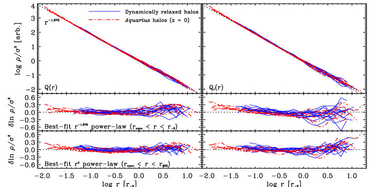
Figure 1: Spherically averaged pseudo-phase-space density profiles for the 21 dark matter halos in our sample. The six level-2 Aquarius halos are shown at $z=0$ (red dot-dashed lines), the other fifteen (solid blue) are shown at the most recent redshift when they pass the dynamical relaxation criteria (Sec. 2.4.3). Left panels correspond to $Q(r)\equiv\rho/\sigma^{3}$; panels on the right correspond to the “radial” $Q_{r}(r)\equiv\rho/\sigma_{r}^{3}$. Radii are scaled to the scale radius, $r_{-2}$, of each halo. Middle panels show residuals from the best $r^{-1.875}$ power-law fit to the $r_{\rm conv}<r<r_{-2}$ portion of the profiles. These best fits are also used to choose the vertical normalization of each profile in the upper panels, so as to minimize the halo-to-halo scatter in the inner profiles. Bottom panels are analogous to the middle ones, but for power-law fits over the whole range $r_{\rm conv}<r<r_{200}$, with free-floating exponent, $r^{\chi}$. Values of $\chi$ and $\chi_{r}$ for each halo are listed in Table 2.

2 The Simulations

We study the formation of $21$ CDM halos selected from a $100\,h^{-1}$ Mpc-box cosmological simulation and resimulated at high resolution in their full cosmological context. We provide below a brief summary of the numerical techniques, including the adopted cosmological parameters; the initial conditions setup; the simulation code; as well as the halo selection criteria and analysis techniques. More detailed information about our resimulation and analysis techniques may be found in previous papers by our group (e.g., Power et al., 2003; Navarro et al., 2004; Springel et al., 2008; Navarro et al., 2008).

2.1 Cosmological Parameters

All our simulations adopt the currently favored $\Lambda$CDM cosmogony with the following parameters: $\Omega_{\rm M}=0.25$, $\Omega_{\Lambda}=1-\Omega_{\rm M}=0.75$, $\sigma_{8}=0.9$, $n_{s}=1$, and a Hubble constant $H_{0}=H(z=0)=100\,h$ km s^-1 Mpc${}^{-1}=73$ km s^-1 Mpc^-1. These parameters are the same as those adopted for the Millennium Simulation (Springel et al., 2005), and are consistent (within 2-sigma) with those derived from the WMAP 1- and 5-year data analyses (Spergel et al., 2003; Komatsu et al., 2009) and with the recent cluster abundance analysis of Henry et al. (2009).

2.2 Halo Selection

The $21$ halos were selected from the same $900^{3}$-particle, $100\,h^{-1}$ Mpc-box parent simulation used for the Aquarius Project (Springel et al., 2008). These halos were subsequently resimulated at higher resolution using the technique described in detail by Power et al. (2003). We avoid halos that form in the periphery of much larger systems by imposing a mild isolation criterion so that no halo more massive than half the mass of the selected system lies within $1\,h^{-1}$ Mpc at $z=0$. This parent simulation was later also resimulated in its entirety at much higher resolution; this is the Millennium-II Simulation recently analyzed by Boylan-Kolchin et al. (2009).

Besides the six Aquarius halos, which were all selected to have virial masses of order $\sim 10^{12}\,h^{-1}M_{\odot}$, we have resimulated a further set of $15$ halos in order to span the mass range $\sim 10^{12}$ to a few times $10^{14}\,h^{-1}M_{\odot}$. These $15$ simulations have typically a few million particles within the virial radius at $z=0$ and are of lower numerical resolution than the level-2 Aquarius halos. Combining these two datasets allows us to assess the sensitivity of our results to numerical resolution. Table 1 lists the main properties of each halo in our sample.

2.3 The Code

All simulations were run with either the publicly available GADGET-2 code (Springel, 2005) or its latest version, GADGET-3, which was developed for the Aquarius Project. Softening lengths are chosen according to the “optimal” prescription of Power et al. (2003). Pairwise interactions are fully Newtonian for separations exceeding the spline-lengthscale $h_{s}$. Table 1 quotes the equivalent Plummer softening, $\epsilon_{G}=h_{s}/2.8$, for each resimulated halo. Throughout the simulations, the softening length is kept fixed in comoving coordinates.

2.4 Analysis

2.4.1 Spherically-averaged $Q$ profiles

In order to compute the spherically-averaged pseudo-phase-space density profile of each halo we first identify the halo center with the location of the particle having the minimum potential energy. Then we compute $Q(r)$ in $N_{\rm bin}$ spherical shells equally spaced in $\log_{10}r$ in the range $r_{\rm conv}\leq r\leq r_{200}$. Here $r_{\rm conv}$ is the convergence radius defined by Power et al. (2003), where circular velocities converge to better than $10\%$ (see also Navarro et al., 2008). For each spherical shell (radial bin), we estimate $Q(r)=\rho/\sigma^{3}$, where $\rho$ is just the mass of the shell divided by its volume and $\sigma^{2}$ is twice the specific kinetic energy in the shell. We also compute a “radial” $Q$ estimate, $Q_{r}(r)=\rho/\sigma_{r}^{3}$ in an analogous way, although instead of the total kinetic energy we use only the kinetic energy in radial motions to estimate $\sigma_{r}$.

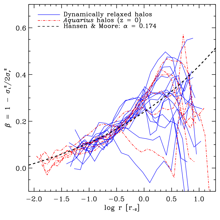
Figure 2: Radial profiles of the velocity anisotropy parameter, $\beta=1-\sigma_{t}^{2}/2\sigma_{r}^{2}$, for all halos in our sample. Line types are as in Fig. 1. Radii are normalized to the scale radius of each halo. Note the non-monotonic radial dependence of $\beta$: halos are nearly isotropic near the center, radially biased near $r_{-2}$, but approximately isotropic again in the outskirts. The anisotropy expected from the $\beta(\gamma)$ relation of Hansen & Moore (2006) for an Einasto profile with $\alpha=0.174$ is also shown.

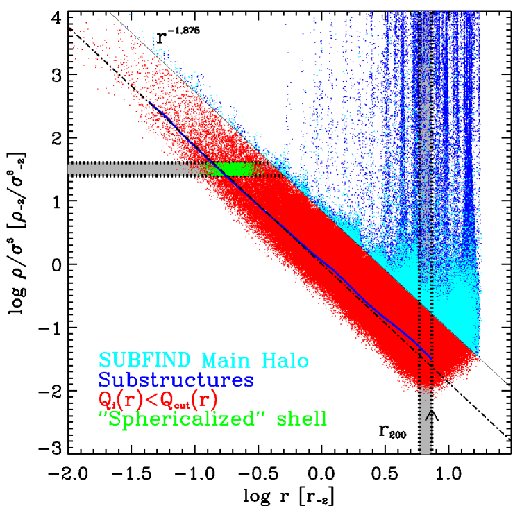
Figure 3: “Local” estimates of the pseudo-phase-space density, $Q_{i}$, as a function of distance from the halo centre for all halo particles in one of our simulations. Different colors correspond to various particle subsamples. (i) Blue denotes particles in self-bound substructures, as identified by SUBFIND. (ii) Cyan indicates particles not bound to any substructure but with higher-than-average $Q_{i}$ for their location in the halo. These are particles in recently-stripped tidal streams which, although assigned to the main halo by SUBFIND, have yet to phase mix within the main halo (Maciejewski et al., 2009). (iii) Red dots indicate particles with $Q_{i}<Q_{\rm cut}(r)$, which we define as belonging to the relaxed main halo (see Fig. 4). Also plotted are the spherically-averaged $Q(r)$ profile (solid blue line), and the best-fit $r^{-1.875}$ power law (dot-dashed line). Vertical and horizontal bands show, respectively, the particles selected for Figs. 4 and  5.

2.4.2 Local $Q$ profiles

A different estimate of the pseudo-phase-space density may be obtained, for each shell, by considering “local” estimates of $Q$ at the position of each particle. We shall call this $Q_{i}=\rho_{i}/\sigma_{i}^{3}$, and use $N_{\rm ngb}$ nearest neighbours in order to compute the local density and velocity dispersion. Density estimates at the location of the $i^{th}$ particle are computed as

$$\rho_{i}=\sum_{j=1}^{N}m_{j}W(|{\mn@boldsymbol{r}}_{i,j}|,h_{i}),$$ (1)

where ${\mn@boldsymbol{r}}_{i,j}\equiv{\mn@boldsymbol{r}}_{i}-{\mn@boldsymbol{r}}_{j}$, and $W(r,h)$ is the smoothing kernel often adopted in Smoothed Particle Hydrodynamics (SPH) simulations:

$$W(r,h)=\frac{8}{\pi h^{3}}\left\{\begin{array}[]{ll}1-6\left(\frac{r}{h}\right)^{2}+6\left(\frac{r}{h}\right)^{3},&0\leq\frac{r}{h}\leq\frac{1}{2},\\ 2\left(1-\frac{r}{h}\right)^{3},&\frac{1}{2}<\frac{r}{h}\leq 1,\\ 0,&\frac{r}{h}>1.\end{array}\right.$$ (2)

The smoothing length, $h_{i}$, of each particle is defined implicitly by the smallest volume that contains $N_{\rm ngb}$ nearest neighbours:

$$h_{i}=\biggl{(}N_{\rm ngb}\frac{3}{4\pi}\frac{m_{i}}{\rho_{i}}\biggr{)}^{1/3}.$$ (3)

We use, as default, $N_{\rm ngb}=48$ for our lower resolution runs and $64$ for the level-2 Aquarius halos.

Given $N_{\rm ngb}$, the local velocity dispersion for particle $i$ is given by $\sigma_{i}^{2}=\overline{v^{2}}-\overline{v}^{2}$, where the unweighted averages are computed over all $N_{\rm ngb}$ neighbours.

2.4.3 Relaxation criteria

In order to minimize the effect of transient, rapidly-evolving evolutionary stages, such as ongoing mergers, we impose (when explicitly stated) relaxation criteria similar to those introduced by Neto et al. (2007). These include restrictions on the fraction of the virial mass in self-bound substructures, $f_{\rm sub}=M_{\rm sub}(r<r_{200})/M_{200}<0.07$; on the offset between the center of mass of the halo and its true centre (as defined by the particle with minimum potential energy), $d_{\rm off}=|{\mn@boldsymbol{r}}_{\rm CM}-{\mn@boldsymbol{r}}_{\rm cen}|/r_{200}<0.05$, and on the virial ratio of kinetic to potential energies, $2K/|\Phi|<1.3$.

In practice, when a halo does not satisfy the relaxation criteria at $z=0$ we track its main progenitor back in time until we find the first snapshot when it does. This typically occurs at redshifts less than $\sim 0.2$, but in one case we had to go back in time until $z\sim 0.8$ in order to find a suitably “relaxed” configuration. In what follows, we shall consider relaxed configurations only for the lower-resolution halos but take the $z=0$ configuration for the Aquarius halos. As we show below, the results are similar in the two cases, which means that our conclusions are not particularly sensitive to our requirement of dynamical equilibrium.

The properties of each halo in our sample at $z=0$ are listed in Table 1. Here we list the virial mass, $M_{200}$, the virial radius, $r_{200}$, the number of particles ($N_{200}$) within $r_{200}$, as well as the gravitational softening, $\epsilon_{G}$, and the convergence radius, $r_{\rm conv}$. The peak of the circular velocity curve is also specified by $r_{\rm max}$ and $V_{\rm max}$.

3 Pseudo-Phase-Space Density Profiles

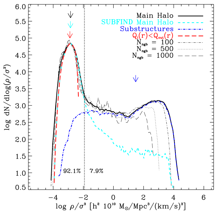
Figure 4: Distribution of local phase-space densities, $Q_{i}$, for particles in the thin (shaded) spherical shell near the virial radius of the halo shown in Fig. 3. Substructures identified by SUBFIND are shown in blue, the main SUBFIND halo in cyan. Various thin lines illustrate the effect of varying the number of neighbours in the $\rho_{i}$ and $\sigma_{i}$ estimates, as labelled in the legend. As discussed in the text, a simple cut $Q_{i}<Q_{\rm cut}$ identifies unequivocally all well-mixed particles in the main halo; $Q_{\rm cut}$ is shown by the vertical dotted line. Down-pointing arrows indicate the median of the distribution of each set of particles. Because there are few particles in the high-$Q_{i}$ tail, the median $Q_{i}$ of the main SUBFIND halo and that of particles with $Q_{i}<Q_{\rm cut}$ are nearly identical. We adopt the latter as the characteristic pseudo-phase-space density of the smooth halo at each radius.

3.1 Spherically-averaged Q profiles

Figure 1 shows the spherically-averaged $Q(r)$ profiles for all halos in our sample, together with residuals from various best-fits. Panels on the left and on the right correspond to $Q(r)$ and $Q_{r}(r)$, respectively. The plotted profiles extend from the convergence radius, $r_{\rm conv}$, to the virial radius, $r_{200}$. Middle panels show residuals from best fits to the region inside $r_{-2}$ with an $r^{-1.875}$ power law. All profiles are normalized to the scale radius, $r_{-2}$, and vertically according to the power-law best fit. Bottom panels show residuals from fits to the $r_{\rm conv}<r<r_{200}$ profile with a power law with free-floating exponent, $Q\propto r^{\chi}$.

A few things are worth noting in this figure. The first is how closely both the $Q(r)$ and $Q_{r}(r)$ profiles follow simple power laws, from the innermost resolved radius out to $r_{200}$. In the case of $Q(r)$, even when the exponent of the fit is fixed at $\chi=-1.875$, which means that a single free parameter (the vertical normalization) is allowed, residuals from best fits do not exceed $\sim 30\%$ anywhere within the virial radius. This power-law behaviour holds for roughly three decades in $r$ and six decades in $Q$.

Although the best-fit $\chi$ differs from $-1.875$ (see Table 2 for actual values), the residuals decrease only very slightly when allowing $\chi$ to float freely. Defining a figure-of-merit function as

$$\psi^{2}={1\over N_{\rm bins}}\sum_{1}^{N_{\rm bins}}(\ln Q-\ln Q_{\rm fit})^{2},$$ (4)

we find that $\psi$, averaged over all halos and fit over the range $r_{\rm conv}<r<r_{200}$, varies only from $\langle\psi\rangle=0.102$ when fixing $\chi=-1.875$ to $\langle\psi\rangle=0.085$ when allowing $\chi$ to be a free parameter.

The “tilt” in the $Q_{r}$-residuals shown in the middle-right panel of Figure 1 indicates that the $\chi_{r}$ exponent that fits best the $Q_{r}(r)$ profiles is slightly more negative than $-1.875$. Overall, however, $Q_{r}(r)$ may also be approximated with a power law with $\chi_{r}\approx 1.92$, as may be seen in the bottom right panel of the same figure. The average $\psi$ for power-law fits with variable $\chi_{r}$ is $0.142$, which means that $Q_{r}(r)$ deviates more than $Q(r)$ from a simple power law, but only slightly so.

The reason why $Q_{r}(r)$ deviates more from a simple power law than $Q(r)$ may be traced to the complex behaviour of the anisotropy parameter, $\beta(r)=1-\sigma_{\rm t}^{2}/2\sigma_{r}^{2}$. All halos in our sample are almost isotropic near the center, radially anisotropic further out, but nearly isotropic again close to the virial radius. Because of this complex radial behaviour, $Q(r)$ and $Q_{r}(r)$ cannot both be simultaneously well fitted by a power law with the same exponent.

Although power laws provide excellent fits to the pseudo-phase-space density profiles, further scrutiny of the middle and lower panels of Fig. 1 reveals a well defined trend in the residuals of most halos, which tend to “curve up” slightly but significantly in the outer regions and, to a lesser extent, in the innermost regions as well. The latter deviations are best appreciated in the Aquarius halos, which have much better resolution than the rest.

These results seem to apply both to the Aquarius halos and to the dynamically-relaxed halo sample, which suggests that our conclusions are not crucially dependent on the adoption of the particular relaxation criteria we used to select the sample. The above-noted trend in the residuals means that the exponent, $\chi$, derived from $r^{-\chi}$ power-law fits will depend on the radial range adopted for the fit.

Given the desirable properties of a simple power law, it is worth investigating whether the deviations from a simple $r^{\chi}$ behaviour might be due to the presence of substructure or to the aspherical nature of halo structure. We explore these possibilities next.

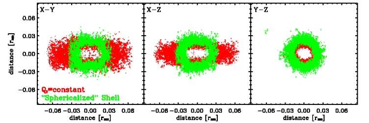
Figure 5: Orthogonal projections of particles in a shell of roughly constant pseudo-phase-space density (i.e., those in the horizontal shaded band in Figure 3, excluding substructures). For clarity, we plot in each panel only particles in a thin slice perpendicular to the viewing axis. Red points show the original positions; these delineate a nearly prolate ellipsoid, which has been rotated so that its principal axes coincide with the coordinate axes of the plot. Green points show the projected particle positions after correcting for triaxiality by the method outlined in the text.

3.2 Local Q profiles

Fig. 3 shows $Q_{i}$, the local estimate of $Q$ at the location of each particle in the halo, as a function of the distance from the halo centre. Because substructures are overdense and have lower velocity dispersion than their immediate surroundings, they show up prominently in this plot as particles with very high $Q_{i}$ at a given radius. This is confirmed by the color coding adopted in the figure: particles in dark blue are those associated by the substructure-finder SUBFIND (Springel et al., 2001) to self-bound subhalos that survive within the main halo. Clearly, because their pseudo-phase-space density is so distinct from the main halo, substructures have the potential to bias estimates of $Q(r)$, especially in the outer regions, where subhalos are more prevalent.

Although it would be simple enough to remove the self-bound structures from $Q(r)$ profiles, the cyan dots in Fig. 3 illustrate a second, related problem. These are particles that SUBFIND associates with the main halo, but which clearly have deviant $Q_{i}$ values relative to the surrounding average. As discussed, for example, by Maciejewski et al. (2009), these are particles recently stripped from substructures; although now unbound to any subhalo, they have yet to phase mix fully with the underlying main halo.

Fig. 4 shows the $Q_{i}$ distribution of all particles in the thin spherical shell near the virial radius of the halo shown by the vertical shaded region in Fig. 3. This shows the wide range in $Q_{i}$ (almost 8 decades) spanned by particles at a fixed distance from the halo centre. Despite this, the figure also shows that the characteristic $Q$ at that distance is well defined, since most particles have $Q_{i}$ values close to the peak on the left of the distribution. (Note the logarithmic scale in the $y$-axis.) The tail to the right of this peak contains self-bound substructures (in blue, as identified by SUBFIND) and recently stripped material, which, as mentioned above, are assigned to the main halo by SUBFIND despite their higher-than-average $Q_{i}$ values.

The shape of the distribution suggests that imposing a simple criterion, e.g., $Q_{i}<Q_{\rm cut}$, should be sufficient to identify unequivocally well-mixed particles belonging to the main smooth halo; a plausible choice for $Q_{\rm cut}$ is shown by the vertical dotted line in Fig. 4. Down-pointing arrows indicate the median of the distribution of each set of particles. Note that, because a small fraction of the particles are in the high-$Q_{i}$ tail, the median $Q_{i}$ of the main SUBFIND halo and that of particles with $Q_{i}<Q_{\rm cut}$ are nearly identical.

We therefore adopt the simple $Q_{i}<Q_{\rm cut}$ prescription to define the main “smooth” halo. Once $Q_{\rm cut}$ is chosen at some radius, we may use the approximate power-law behaviour of $Q$ to scale it to any other radius by $Q_{\rm cut}(r)\propto r^{-1.875}$. Particles shown in red in Fig. 3 are those assigned to the smooth halo by this criterion. At each radius, we shall adopt the median $Q_{i}$ of these particles in order to construct the pseudo-phase-space density profile of the main smooth halo. We shall refer to this profile as $Q_{i}^{s}(r)$.

We note that this definition is insensitive to the number of nearest neighbors ($N_{\rm ngb}$) adopted to compute $Q_{i}$: the various lines in Fig. 4 illustrate the results for $N_{\rm ngb}=48$ particles (our default value), as well as for $1000$ (long-dashed), 500 (dotted), and 100 (dot-dashed), respectively.

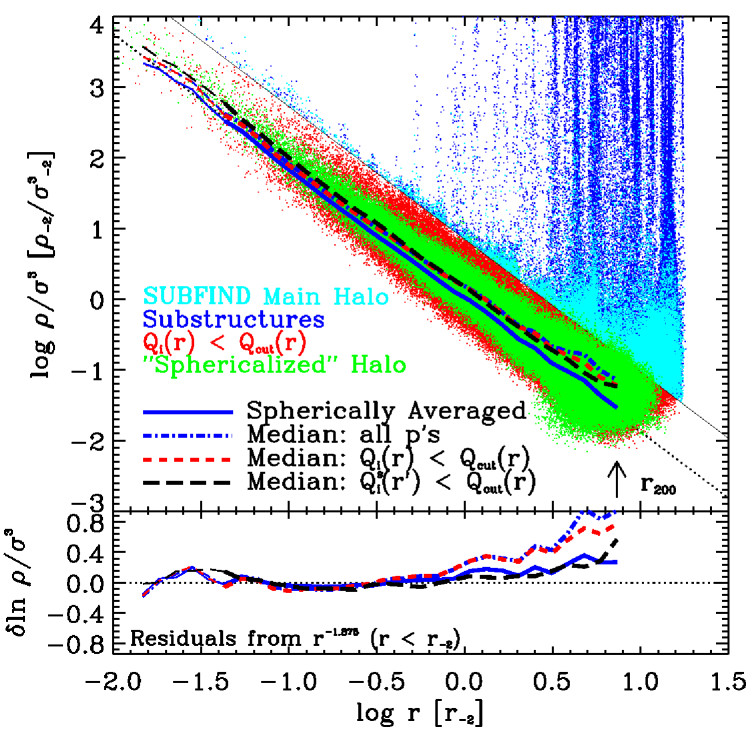
Figure 6: Local pseudo-phase-space density as a function of radius for the same halo shown in Fig. 3. Colored dots are as in Fig. 3. Red and green dots indicate smooth main halo particles before and after correcting for halo shape. The solid curve is the spherically-averaged profile, and is compared with the curves tracing the median $Q_{i}$ for (i) all particles (blue dot-dashed), (ii) all particles in the smooth main halo (red dashed), and (iii) smooth main halo particles corrected for triaxiality (dashed). The dotted line shows a power-law, $r^{-1.875}$.

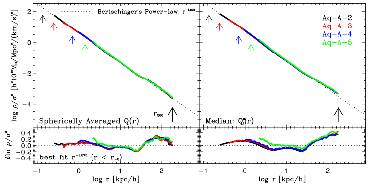
Figure 7: Spherically-averaged (left) and median local (right) pseudo-phase-space density profiles for the convergence series of the Aq-A halo (Springel et al., 2008; Navarro et al., 2008). Different colors correspond to runs with different resolution, as indicated in the legend. Local profiles refer to the median $Q_{i}$ of the smooth main halo as a function of distance to the halo centre. The dotted line is the power-law $Q\propto r^{-1.875}$, scaled to match Aq-A-2 at $r\leq r_{-2}=11.15\,h^{-1}$ kpc. Bottom panels show the residual with respect to this power-law.

3.3 Correction for triaxiality

Dark halos are not spherically symmetric. Because of this, a shell of particles at constant distance from the halo center will have a wide $Q_{i}$ distribution, even if one subtracts substructure as specified in the previous subsection. Iso-$Q$ surfaces track fairly well the isodensity contours of the main halo, and follow closely three-dimensional ellipsoidal surfaces. Fig. 5 shows three orthogonal projections of particles with similar values of $Q_{i}$, selected from those falling in the horizontal band highlighted in Fig. 3. Only particles in the smooth main halo are plotted here. The original particle positions (in red) in a thin slice perpendicular to the line of sight are seen to trace a nearly prolate ellipsoid, which for convenience has been rotated so that its principal axes coincide with the coordinate axes of the projection.

Given that the “iso-$Q$” surfaces are well approximated by ellipsoids, we may use the eigenvalues of the diagonalized inertia tensor to compute an elliptical radius, $r^{\prime}$, for each $Q_{i}$, to define an “ellipsoidal” $Q_{i}(r^{\prime})$ profile that may be contrasted directly with $Q_{i}(r)$. In practice, we slice the smooth main halo in narrow bins in $Q_{i}$; compute the axis lengths $a$, $b$, and $c$; and use them to reassign an ellipsoidal radius $r^{\prime}$ to each particle in the smooth main halo. We compute $r^{\prime}$ as

$$r^{\prime 2}=\biggr{(}\frac{x}{a}\biggl{)}^{2}+\biggr{(}\frac{y}{b}\biggl{)}^{2}+\biggr{(}\frac{z}{c}\biggl{)}^{2},$$ (5)

after normalizing $a$, $b$, and $c$ so that $abc=1$ for all shells. This choice preserves the typical distance to the halo centre of particles in a given $Q_{i}$ shell. The result of the procedure is illustrated in Fig. 5, where the green dots are the same particles as those shown in red, but the coordinate axes are now $x^{\prime}=x/a$, $y^{\prime}=y/b$ and $z^{\prime}=z/c$.

The green dots in Fig. 6 delineate the $Q_{i}^{s}(r^{\prime})$ profile for the smooth main halo. The lines in Fig. 6 show the variations in the pseudo-phase-space density profile induced by the various alternative ways of estimating distances and $Q$ that we have discussed so far.

Although the profiles change appreciably, they all show the same upturn in the outer regions, relative to a simple $r^{-1.875}$ power-law fit, noted when discussing the spherically-averaged $Q(r)$ profiles (Sec. 3.1). The upturn is indeed more pronounced when using local-$Q$ estimates, because (i) local densities are sensitive to inhomogeneities and are therefore higher than the spherical average, and (ii) because local $\sigma$ estimates are lower than the spherical average, since they do not include the bulk motion of subhalos and recently stripped material. Interestingly, Fig.  6 shows that, after correcting for triaxiality, the spherically-averaged profile is indistinguishable from the $Q_{i}^{s}(r^{\prime})$ profile. We conclude that the upturn is not caused by the presence of substructures in the outer regions nor by departures from spherical symmetry. We discuss the interpretation of this robust feature of the $Q$ profiles next.

3.4 Numerical convergence

Before considering the meaning of the departures of $Q$ profiles from simple power laws we should check explicitly that our conclusions are not affected by the numerical resolution of the simulations. We show this in Fig. 7, where we compare the $Q(r)$ and $Q_{i}^{s}(r)$ profiles of one of the Aquarius halos at four different resolutions. The highest, Aq-A-2, has more than $100$ million particles within the virial radius; the lowest, Aq-A-5, about $600$ thousand. The non-Aquarius halos in the series analyzed in this paper have numerical resolution comparable to Aq-A-4. Fig. 7 shows convincingly that our results are unlikely to be adversely affected by numerical resolution. Both the spherically-averaged and the local pseudo-phase-space density profiles are very well reproduced at all radii, down to the inermost resolved radius, $r_{\rm conv}$, of each run.

3.5 Comparison with Bertschinger’s similarity solution

The local pseudo-phase-space density profiles for the smooth main halo of all our systems is shown in Fig. 8. The profiles are shown as a function of the elliptical radius (eq. 5), scaled to the scale radius of each halo, $r_{-2}$. All profiles have been normalized vertically so that they coincide at $r^{\prime}=r_{-2}$. The dotted line shows a $Q\propto r^{-1.875}$ power law, also normalized at $r_{-2}$. The bottom panel shows residuals relative to the $r^{-1.875}$ power law.

Fig. 8 shows the main result of our analysis. The pseudo-phase-space density profiles of our simulated halos clearly deviate from a simple power law in the outer regions. This deviation is actually predicted by the secondary infall similarity solution of Bertschinger (1985). Indeed, in the similarity solution the $Q\propto r^{-1.875}$ behaviour occurs only asymptotically in the inner regions of the halo. In the outer regions, and more precisely, near the location of the “shock radius”, $r_{\rm shock}$ (for collisional fluids), or, equivalently, of the first infall caustic (for collisionless fluids), the pseudo-phase-space density profile (or entropy profile in the case of a collisional fluid) shows a clear upturn from the inner asymptotic power-law behaviour.

The reason for this upturn is that the fluid is not fully virialized near $r_{\rm shock}$, since this radius marks the transition between mass shells that are infalling for the first time and those that have already crossed (or shocked) material that collapsed earlier. For example, in the case of collisionless fluids, a mass shell must cross the center and complete roughly 2-3 full oscillations before settling onto a periodic orbit of constant apocenter. In the case of a collisional fluid, a newly shocked shell drifts inward from the radius at which it was shocked before reaching hydrostatic equilibrium (see Fig. 4 of Bertschinger 1985). As a result, $Q(r)$ (or the “entropy” in the case of a collisional fluid) shows a characteristic upturn at $r_{\rm shock}$ like the one shown in Fig. 8.

As discussed by White et al. (1993), the first caustic/shock, which occurs at about a third of the current turnaround radius, lies close to the virial radius, as defined here. Given that our halos have concentrations, $c=r_{200}/r_{-2}$, of order $7$-$10$ (Neto et al., 2007), we would then expect the upturn in the $Q$ profiles to occur roughly at $\sim 7$-$10\,r_{-2}$.

The dashed black curves in Fig. 8 show the similarity solution, assuming $r_{\rm shock}=8\,r_{-2}$, and normalized vertically at $r=r_{-2}$ to coincide with the simulated halo profiles. It is clear from Fig. 8 that the similarity solution is in excellent agreement with the $Q$ profiles of our simulated halos. This suggests that the upturn in the outer $Q$ profiles just reflects the fact that the regions around the virial radius have not yet fully virialized.

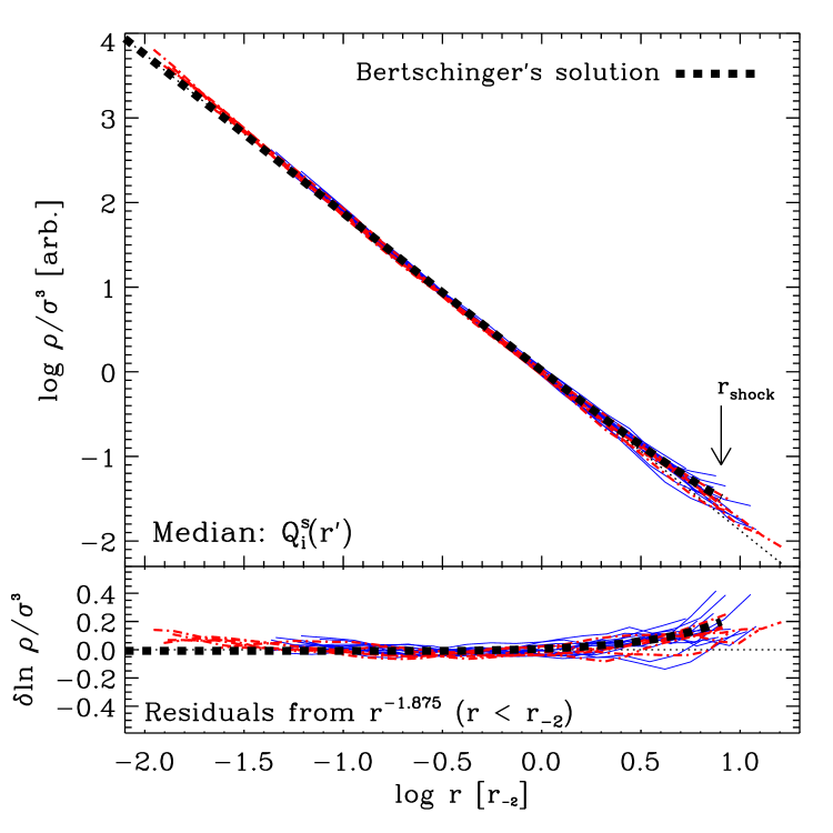
Figure 8: Local estimates of the pseudo-phase-space density as a function of the ellipsoidal radius $r^{\prime}$ (eq. 5). Each curve traces the median $Q_{i}^{s}(r^{\prime})$ for smooth main halo particles, computed in $r^{\prime}$ bins of equal logarithmic width. Radii are scaled to the value of $r_{-2}$ of each halo. The dotted line shows the $Q\propto r^{-1.875}$ power law, whereas the thick dashed black curve shows the actual similarity solution computed by Bertschinger (1985). The outermost point of this solution, indicated by the downward pointing arrow, corresponds to $r_{\rm shock}$, the “shock radius” (for collisional fluid infall) or to the position of the first caustic (for collisionless fluids). Radii for the similarity solution assume $r_{\rm shock}=8\,r_{-2}$ All profiles are normalized at $r^{\prime}=r_{-2}$. Note that halo profiles deviate from the asymptotic inner $r^{-1.875}$ power law in the same way as the similarity solution.

4 Summary

We have used a set of 21 high-resolution cosmological N-body simulations to investigate the pseudo-phase-space density profiles, $Q(r)=\rho/\sigma^{3}$, of cold dark matter halos. In particular, we concentrate our analysis on the radial dependence of $Q$ for particles in the smooth main halo component, after carefully removing substructures and correcting for halo shape.

Our main result is that although $Q(r)$ is remarkably well-approximated by a power law, a slight but systematic upturn from the power-law profile is clearly seen in the outer regions of all our simulated halos. Both the exponent of the power law, as well as the upturn in the outer regions are consistent with the particular secondary infall similarity solutions derived by Bertschinger (1985). In these solutions, the power-law inner region corresponds to the virialized region of the halo, whereas the upturn in the outer regions coincides with the location of the shock/first caustic of the system or, roughly speaking, with the virial boundary of a halo. Although Bertschinger’s is just one particular secondary-infall similarity solution, valid in the simple case of a point-mass perturber in an Einstein-de Sitter universe, the upturn in Q marking the virial boundary of the system is expected to be a general feature of such solutions.

Although the outer upturn may be robust, the fact that the exponent of the inner power law is consistent with Bertschinger’s ($\chi\sim-1.875$) is somewhat surprising. As shown by Fillmore & Goldreich (1984), the non-linear structure of halos formed through self-similar secondary infall depend on the scaling index that characterizes the mass dependence of the initial perturbation, $\delta M/M\propto M^{-\epsilon}$. In the case of Bertschinger’s solution $\epsilon=1$, but this is a poor approximation to the typical overdensity that seeds the collapse of galaxy-sized LCDM halos. The agreement between Bertschinger’s $Q(r)$ and the simulated profiles is therefore a non-trivial result whose significance remains unclear.

The presence of the upturn in the $Q(r)$ profiles casts doubts on work that attempts to construct dynamical equilibrium models of CDM halos by assuming that the power-law behaviour of $Q$ profiles applies to all radii (see, e.g., Austin et al., 2005; Dehnen & McLaughlin, 2005). The $r^{\chi}$ behaviour seems to hold only in the inner regions, and our results caution against fitting power laws to $Q(r)$ over a radial range that extends outside the scale radius.

Because the radius where the upturn becomes noticeable marks the transition to the region where virial equilibrium no longer holds, this radius, expressed as a fraction of the virial radius, may vary systematically with halo mass, collapse time, or cosmological parameters. Indeed, the virial radius definition we adopt here does not depend on the formation history of each object, but the boundary of the region where virial equilibrium might hold does. For example, the shock radius of an early collapsing halo that has accreted little mass in the recent past might occur further away (in units of $r_{200}$) than another system of similar mass that has assembled a considerable fraction of its present-day mass more recently. It may be worth checking whether the trends of $\chi$ with power spectrum and mode of assembly noted in the literature (see, e.g., Knollmann et al., 2008; Wang & White, 2009) might be explained by this process.

Finally, we note that our highest resolution halos (those from the Aquarius project) also present evidence of departures from a simple power-law $Q$ profile near the innermost resolved radius. At the moment it is unclear whether this indicates that the power-law behaviour of $Q(r)$ is just an approximation that breaks down inside some characteristic radius, or whether estimates of $Q(r)$ at those radii might be affected by numerical uncertainties. For example, it is easy to demonstrate that an isotropic halo whose mass profile follows strictly an Einasto law cannot have a power-law $Q(r)$ law that extends all the way to the centre (see, e.g., Ma et al., 2009). The radial dependence of these $Q(r)$ profiles may be more accurately represented by an Einasto-like form where the power-law index changes gradually but smoothly with radius. We plan to address this and other pertinent issues in forthcoming work.

Table 1: We list, for each halo in our sample, a label, the Plummer-equivalent gravitational softening and convergence radius, as well as the virial radius at $z=0$. The structural parameters $V_{\rm max}$ and $r_{\rm max}$ identify the peak of the circular velocity curve for each halo. Finally, $M_{200}$ is the virial mass and $N_{200}$ is the number of particles within the virial radius. The $z_{\rm rel}$ column specifies, for non-Aquarius halos, the redshift of the most recent snapshot when the halo satisfies the relaxation criteria introduced in Sec. 2.4.3.

Halo	$\epsilon_{G}$	$r_{\rm conv}$	$r_{200}$	$r_{\rm max}$	$V_{\rm max}$	$M_{200}$	$N_{200}$	$z_{\rm rel}$
	[kpc/h]	[kpc/h]	[kpc/h]	[kpc/h]	[km/s]	$[10^{10}M_{\odot}/h]$	$[10^{6}]$
Aq-A-2	4.8$\times 10^{-2}$	0.250	179.5	20.5	208.5	134.5	134.5	-
Aq-B-2	4.8$\times 10^{-2}$	0.219	137.0	29.3	157.7	59.8	127.1	-
Aq-C-2	4.8$\times 10^{-2}$	0.248	177.3	23.7	222.4	129.5	126.8	-
Aq-D-2	4.8$\times 10^{-2}$	0.281	177.3	39.5	203.2	129.5	127.0	-
Aq-E-2	4.8$\times 10^{-2}$	0.223	155.0	40.5	179.0	86.5	123.6	-
Aq-F-2	4.8$\times 10^{-2}$	0.209	152.7	31.2	169.1	82.8	167.5	-
h1	0.39	1.090	134.4	44.0	151.9	56.4	2.04	0.198
h2	0.25	0.852	144.6	35.1	159.9	70.3	4.91	0.000
h3	0.38	1.063	154.1	33.7	178.6	85.0	2.60	0.049
h4	0.31	0.899	154.7	30.3	175.8	86.1	4.17	0.876
h5	0.24	0.797	156.1	32.0	174.8	88.5	6.10	0.000
h6	0.26	0.829	158.0	47.3	171.6	91.7	6.00	0.000
h7	0.35	1.001	158.3	37.4	184.8	92.2	3.25	0.062
h8	0.39	1.148	175.6	39.1	203.5	125.9	3.30	0.350
h9	0.45	1.351	177.8	45.1	200.2	130.8	2.48	0.000
h10	0.33	0.944	183.7	21.3	209.2	144.1	4.79	0.350
h11	1.06	3.239	275.5	188.2	285.6	486.4	1.08	0.309
h12	1.39	4.006	391.0	114.2	425.6	1389.5	1.26	0.140
h13	1.61	4.418	396.1	86.9	422.9	1445.2	0.98	0.140
h14	2.08	6.886	856.0	263.6	888.2	14581.8	2.62	0.030
h15	3.65	11.595	981.6	444.8	1043.0	21993.1	1.16	0.094

Table 2: Values of the exponent $\chi$ obtained from $r^{\chi}$ fits to various $Q$ profiles, as indicated in the legend. $\chi_{r}$ refers to fits to the “radial” $Q_{r}$ profiles. The average $\chi$ for all halos is listed in the next-to-last row, together with its standard deviation . The average figure-of-merit for all halos, $\langle\psi_{\rm min}\rangle$, is listed in the last row of the table.

	Spherically averaged: $Q(r)$, $Q_{r}(r)$							Median: $Q^{\rm s}_{\rm i}(r)$
Halo	$\chi$		$\chi_{\rm r}$		$\chi$		$\chi_{\rm r}$	$\chi$	$\chi$
	($r_{\rm conv}<r<r_{-2}$)				($r_{\rm conv}<r<r_{200}$)			($r_{\rm conv}<r<r_{-2}$)	($r_{\rm conv}<r<r_{200}$)
Aq-A-2	-1.917		-1.976		-1.873		-1.955	-1.910	-1.821
Aq-B-2	-1.868		-1.938		-1.832		-1.872	-1.914	-1.808
Aq-C-2	-1.948		-2.010		-1.883		-1.948	-1.932	-1.823
Aq-D-2	-1.862		-1.942		-1.831		-1.901	-1.939	-1.804
Aq-E-2	-1.912		-1.947		-1.894		-1.902	-1.863	-1.853
Aq-F-2	-1.911		-1.980		-1.885		-1.954	-1.965	-1.823
h1	-1.826		-1.847		-1.858		-1.813	-1.798	-1.792
h2	-1.862		-1.920		-1.811		-1.908	-1.828	-1.696
h3	-1.993		-2.076		-1.864		-1.903	-1.967	-1.800
h4	-1.895		-1.942		-1.863		-1.943	-1.879	-1.766
h5	-1.916		-1.999		-1.872		-1.938	-1.887	-1.771
h6	-1.898		-2.010		-1.863		-1.908	-1.856	-1.801
h7	-1.960		-1.918		-1.940		-1.957	-1.878	-1.863
h8	-1.864		-1.951		-1.808		-1.916	-1.871	-1.727
h9	-1.869		-1.953		-1.858		-1.926	-1.846	-1.792
h10	-1.975		-2.042		-1.871		-1.991	-1.972	-1.754
h11	-1.896		-2.008		-1.843		-1.845	-1.903	-1.756
h12	-1.879		-1.949		-1.875		-2.023	-1.864	-1.758
h13	-1.843		-1.955		-1.847		-1.882	-1.768	-1.724
h14	-1.810		-1.902		-1.817		-1.886	-1.801	-1.732
h15	-1.847		-1.966		-1.835		-1.919	-1.765	-1.648
$\langle\chi\rangle$	$-1.893\pm 0.048$		$-1.963\pm 0.050$		$-1.858\pm 0.031$		$-1.919\pm 0.047$	$-1.876\pm 0.061$	$-1.777\pm 0.052$
$\langle\psi_{\rm min}\rangle$	$4.3(\pm 1.3)\times 10^{-2}$		$5.38(\pm 0.16)\times 10^{-1}$		$8.46(\pm 2.1)\times 10^{-2}$		$1.42(\pm 0.50)\times 10^{-1}$	$4.23(\pm 1.79)\times 10^{-2}$	$1.18(\pm 0.43)\times 10^{-1}$

References

- Allgood et al. (2006) Allgood B., Flores R. A., Primack J. R., Kravtsov A. V., Wechsler R. H., Faltenbacher A., Bullock J. S., 2006, MNRAS, 367, 1781
- Arad et al. (2004) Arad I., Dekel A., Klypin A., 2004, MNRAS, 353, 15
- Ascasibar & Binney (2005) Ascasibar Y., Binney J., 2005, MNRAS, 356, 872
- Ascasibar et al. (2007) Ascasibar Y., Hoffman Y., Gottlöber S., 2007, MNRAS, 376, 393
- Austin et al. (2005) Austin C. G., Williams L. L. R., Barnes E. I., Babul A., Dalcanton J. J., 2005, ApJ, 634, 756
- Barnes et al. (2006) Barnes E. I., Williams L. L. R., Babul A., Dalcanton J. J., 2006, ApJ, 643, 797
- Bertschinger (1985) Bertschinger E., 1985, ApJS, 58, 39
- Boylan-Kolchin et al. (2009) Boylan-Kolchin M., Springel V., White S. D. M., Jenkins A., Lemson G., 2009, MNRAS, 398, 1150
- Dehnen & McLaughlin (2005) Dehnen W., McLaughlin D. E., 2005, MNRAS, 363, 1057
- Diemand et al. (2008) Diemand J., Kuhlen M., Madau P., Zemp M., Moore B., Potter D., Stadel J., 2008, Nature, 454, 735
- Faltenbacher et al. (2007) Faltenbacher A., Hoffman Y., Gottlöber S., Yepes G., 2007, MNRAS, 376, 1327
- Fillmore & Goldreich (1984) Fillmore J. A., Goldreich P., 1984, ApJ, 281, 1
- Frenk et al. (1988) Frenk C. S., White S. D. M., Davis M., Efstathiou G., 1988, ApJ, 327, 507
- Gao et al. (2008) Gao L., Navarro J. F., Cole S., Frenk C. S., White S. D. M., Springel V., Jenkins A., Neto A. F., 2008, MNRAS, 387, 536
- Hansen & Moore (2006) Hansen S. H., Moore B., 2006, New Astronomy, 11, 333
- Hayashi et al. (2007) Hayashi E., Navarro J. F., Springel V., 2007, MNRAS, 377, 50
- Hayashi & White (2008) Hayashi E., White S. D. M., 2008, MNRAS, 388, 2
- Henry et al. (2009) Henry J. P., Evrard A. E., Hoekstra H., Babul A., Mahdavi A., 2009, ApJ, 691, 1307
- Jing & Suto (2002) Jing Y. P., Suto Y., 2002, ApJ, 574, 538
- Klypin et al. (1999) Klypin A., Kravtsov A. V., Valenzuela O., Prada F., 1999, ApJ, 522, 82
- Knollmann et al. (2008) Knollmann S. R., Power C., Knebe A., 2008, MNRAS, 385, 545
- Komatsu et al. (2009) Komatsu E., Dunkley J., Nolta M. R., Bennett C. L., Gold B., Hinshaw G., Jarosik N., Larson D., Limon M., Page L., Spergel D. N., Halpern M., Hill R. S., Kogut A., Meyer S. S., Tucker G. S., Weiland J. L., Wollack E., Wright E. L., 2009, ApJS, 180, 330
- Ma et al. (2009) Ma C.-P., Chang P., Zhang J., 2008, ArXiv e-prints, 0907.3144
- Maciejewski et al. (2009) Maciejewski M., Colombi S., Springel V., Alard C., Bouchet F. R., 2009, MNRAS, 396, 1329
- Merritt et al. (2006) Merritt D., Graham A. W., Moore B., Diemand J., Terzić B., 2006, AJ, 132, 2685
- Merritt et al. (2005) Merritt D., Navarro J. F., Ludlow A., Jenkins A., 2005, ApJL, 624, L85
- Moore et al. (1999) Moore B., Quinn T., Governato F., Stadel J., Lake G., 1999, MNRAS, 310, 1147
- Navarro et al. (1996) Navarro J. F., Frenk C. S., White S. D. M., 1996, ApJ, 462, 563
- Navarro et al. (1997) Navarro J. F., Frenk C. S., White S. D. M., 1997, ApJ, 490, 493
- Navarro et al. (2004) Navarro J. F., Hayashi E., Power C., Jenkins A. R., Frenk C. S., White S. D. M., Springel V., Stadel J., Quinn T. R., 2004, MNRAS, 349, 1039
- Navarro et al. (2008) Navarro J. F., Ludlow A., Springel V., Wang J., Vogelsberger M., White S. D. M., Jenkins A., Frenk C. S., Helmi A., 2008, ArXiv e-prints, 0810.1522
- Neto et al. (2007) Neto A. F., Gao L., Bett P., Cole S., Navarro J. F., Frenk C. S., White S. D. M., Springel V., Jenkins A., 2007, MNRAS, 381, 1450
- Power et al. (2003) Power C., Navarro J. F., Jenkins A., Frenk C. S., White S. D. M., Springel V., Stadel J., Quinn T., 2003, MNRAS, 338, 14
- Rasia et al. (2004) Rasia E., Tormen G., Moscardini L., 2004, MNRAS, 351, 237
- Schmidt et al. (2008) Schmidt K. B., Hansen S. H., Macciò A. V., 2008, ApJL, 689, L33
- Sharma & Steinmetz (2006) Sharma S., Steinmetz M., 2006, MNRAS, 373, 1293
- Spergel et al. (2003) Spergel D. N., Verde L., Peiris H. V., Komatsu E., Nolta M. R., Bennett C. L., Halpern M., Hinshaw G., Jarosik N., Kogut A., Limon M., Meyer S. S., Page L., Tucker G. S., Weiland J. L., Wollack E., Wright E. L., 2003, ApJS, 148, 175
- Springel (2005) Springel V., 2005, MNRAS, 364, 1105
- Springel et al. (2008) Springel V., Wang J., Vogelsberger M., Ludlow A., Jenkins A., Helmi A., Navarro J. F., Frenk C. S., White S. D. M., 2008, MNRAS, 391, 1685
- Springel et al. (2008) Springel V., White S. D. M., Frenk C. S., Navarro J. F., Jenkins A., Vogelsberger M., Wang J., Ludlow A., Helmi A., 2008, Nature, 456, 73
- Springel et al. (2005) Springel V., White S. D. M., Jenkins A., Frenk C. S., Yoshida N., Gao L., Navarro J., Thacker R., Croton D., Helly J., Peacock J. A., Cole S., Thomas P., Couchman H., Evrard A., Colberg J., Pearce F., 2005, Nature, 435, 629
- Springel et al. (2001) Springel V., White S. D. M., Tormen G., Kauffmann G., 2001, MNRAS, 328, 726
- Stadel et al. (2008) Stadel J., Potter D., Moore B., Diemand J., Madau P., Zemp M., Kuhlen M., Quilis V., 2008, ArXiv e-prints, 0808.2981
- Taylor & Navarro (2001) Taylor J. E., Navarro J. F., 2001, ApJ, 563, 483
- Tremaine & Gunn (1979) Tremaine S., Gunn J. E., 1979, Physical Review Letters, 42, 407
- Vass et al. (2009) Vass I. M., Valluri M., Kravtsov A. V., Kazantzidis S., 2009, MNRAS, 395, 1225
- Vogelsberger et al. (2009) Vogelsberger M., White S. D. M., Mohayaee R., Springel V., 2009, MNRAS, 400, 2174
- Wang & White (2009) Wang J., White S. D. M., 2009, MNRAS, 396, 709
- White et al. (1993) White S. D. M., Navarro J. F., Evrard A. E., Frenk C. S., 1993, Nature, 366, 429