On broadcast channels with binary inputs and symmetric outputs

Abstract

We study the capacity regions of broadcast channels with binary inputs and symmetric outputs. We study the partial order induced by the more capable ordering of broadcast channels for channels belonging to this class. This study leads to some surprising connections regarding various notions of dominance of receivers. The results here also help us isolate some classes of symmetric channels where the best known inner and outer bounds differ.

1 Introduction

In [1], Cover introduced the notion of a broadcast channel through which one sender transmits information to two or more receivers. For the purpose of this paper we focus our attention on broadcast channels with precisely two receivers.

Definition: A broadcast channel (BC) consists of an input alphabet $\mathcal{X}$ and output alphabets $\mathcal{Y}_{1}$ and $\mathcal{Y}_{2}$ and a probability transition function $p(y_{1},y_{2}|x)$. A $((2^{nR_{1}},2^{nR_{2}}),n)$ code for a broadcast channel consists of an encoder

$$x^{n}:2^{nR_{1}}\times 2^{nR_{2}}\rightarrow\mathcal{X}^{n},$$

and two decoders

$$\hat{{\cal W}}_{1}:\mathcal{Y}_{1}^{n}\rightarrow 2^{nR_{1}}$$

$$\hat{{\cal W}}_{2}:\mathcal{Y}_{2}^{n}\rightarrow 2^{nR_{2}}.$$

The probability of error $P_{e}^{(n)}$ is defined to be the probability that the decoded message is not equal to the transmitted message, i.e.,

$$P_{e}^{(n)}=\mathbf{P}\left(\{\hat{{\cal W}}_{1}(Y_{1}^{n})\neq{\cal W}_{1}\}\cup\{\hat{{\cal W}}_{2}(Y_{2}^{n})\neq{\cal W}_{2}\}\right)$$

where the message is assumed to be uniformly distributed over $2^{nR_{1}}\times 2^{nR_{2}}$.

A rate pair $(R_{1},R_{2})$ is said to be achievable for the broadcast channel if there exists a sequence of $((2^{nR_{1}},2^{nR_{2}}),n)$ codes with $P_{e}^{(n)}\rightarrow 0$. The capacity region of the broadcast channel is the closure of the set of achievable rates. The capacity region of the two-receiver discrete memoryless channel is unknown.

The capacity region is known for lots of special cases where there is a “dominant receiver” such as degraded, less noisy, more capable, essentially less noisy, and essentially more capable. In fact superposition coding is optimal here. An interesting observation in [7] was that the notions of more capable and essentially less noisy may not be compatible with each other.

In this paper, we study in detail the notions of more capable receivers and essentially less noisy receivers by focusing on an important(commonly used in coding theory) class of binary-input symmetric-output(BISO) broadcast channels. We establish a slew of results and some of the interesting ones are summarized below.

1.1 Summary of selected results

Here are some of the results established in this paper.

• Any BISO channel with capacity $C$ is more capable than the binary symmetric channel with capacity $C$. (Corollary 1)

• The binary erasure channel with capacity $C$ is more capable than any BISO channel with capacity $C$. (Corollary 2)

• Any two BISO channels with the same capacity and whose outputs have cardinality at most 3, are more-capable comparable, i.e. one receiver is more capable than the other receiver. (Corollary 3)

• For any two BISO channels with same capacity, a receiver $Y_{1}$ is more capable than receiver $Y_{2}$ if and only if receiver $Y_{2}$ is essentially less noisy than $Y_{1}$. (They go in reverse directions !) (Lemma 4)

• Superposition coding region is the capacity region for a BISO-broadcast channel if any one of the channels is either a BSC or a BEC. (Corollary 4)

• For two BISO channels with the same capacity, superposition coding is optimal if and only if the channels are more capable comparable. (Corollary 5)

• For two BISO channels of same capacity Marton’s inner bound differs from the outer bound[6] unless the channels are more capable comparable (Theorem 3)

• We also show that it suffices to consider $U\to X$ to be BSC when we wish to compute the boundary of the superposition coding region for BISO broadcast channels. (Lemma 8). This vastly generalizes a result of Wyner and Ziv[10] for degraded BSC broadcast channel.

1.2 Preliminaries

Definition 1.

[4] A channel $F_{1}:X\to Y_{1}$ is said to be more capable than the channel $F_{2}:X\to Y_{2}$, denoted $F_{1}\gg F_{2}$, if $I(X;Y_{1})\geq I(X;Y_{2}),\forall p(x)$.

Definition 2.

[7] A class of distributions $\mathcal{P}=\{p(x)\}$ on the input alphabet $\mathcal{X}$ is said to be a sufficient class of distributions for a 2-receiver broadcast channel if the following holds: Given any triple of random variables $(U,V,X)$ satisfying $(U,V)\to X\to(Y_{1},Y_{2})$ forms a Markov chain, there exists a distribution $q(u,v,x)$ (also obeying the Markov relationship $(U,V)\to X\to(Y_{1},Y_{2})$) that satisfies

$$q(x)\in\mathcal{P},$$

$$I(U;Y_{i})_{p}\leq I(U;Y_{i})_{q},~{}i=1,2,$$

$$I(V;Y_{i})_{p}\leq I(V;Y_{i})_{q},~{}i=1,2,$$

$$I(X;Y_{i}|U)_{p}\leq I(X;Y_{i}|U)_{q},~{}i=1,2,$$ (1)

$$I(X;Y_{i}|V)_{p}\leq I(X;Y_{i}|V)_{q},~{}i=1,2,$$

$$I(X;Y_{i})_{p}\leq I(X;Y_{i})_{q},~{}i=1,2,$$

Definition 3.

[7] A channel $F_{1}:X\to Y_{1}$ is essentially less noisy compared to a channel $F_{2}:X\to Y_{2}$, denoted by $F_{1}\succeq F_{2}$, if there exists a sufficient class of distributions $\mathcal{P}$ such that whenever $p(x)\in\mathcal{P}$, for all $U\to X\to(Y_{1},Y_{2})$ we have

$$I(U;Y_{2})\leq I(U;Y_{1}).$$

In this paper, we restrict ourselves to a class ${\cal C}$ of discrete memoryless channels with binary inputs and symmetric outputs(BISO) as defined below.

Definition 4.

A discrete memoryless channel with input alphabet ${\cal X}=\{0,1\}$ and output alphabet ${\cal Y}=\{k:-l\leq k\leq l\}$ is said to belong to class ${\cal C}$ (or BISO) if

$$p_{k}={\rm P}(Y=k|X=0)={\rm P}(Y=-k|X=1),-l\leq k\leq l.$$

Binary symmetric channel(BSC) and Binary Erasure Channel(BEC) are examples of channels that belong to the class ${\cal C}$. It is easy to see that uniform input distribution is the capacity achieving distribution for any channel in ${\cal C}$.

Remark 1.

As $k=0$ can be split equally into $0^{+}$ and $0^{-}$ with probability $p_{0^{+}}=p_{0^{-}}=p_{0}/2$, so we just consider $k=\pm 1,...,\pm l$ and use $\{p_{k},p_{-k}:k=1,\ldots,l\}$ to denote the transition probabilities. Sometimes shortened to $\{p_{k},p_{-k}\}_{k}$.

Partition $P$ of an interval $[a,b]$ is a finite sequence (points) $\{t_{k}\}_{k}$ such that $a=t_{0}<t_{1}<t_{2}<\ldots<t_{N}=b$. A partition $P$ is finer than $Q$ if points of partition $P$ contain those of $Q$. A common refinement of two partitions $P$ and $Q$ is a new partition consisting of all the points of $P$ and $Q$.

Definition 5.

(BISO partition and BISO curve)
For a BISO channel with transition probabilities $\{p_{k},p_{-k}\}_{k}$, rearrange $h(\frac{p_{k}}{p_{k}+p_{-k}})$ in the ascending order and denote the permutation as $\pi$. BISO partition is defined as the partition of $[0,1]$ with points $t_{k}=\sum_{i=1}^{k}(p_{\pi_{i}}+p_{-\pi_{i}})$. We set $t_{0}=0$. BISO curve is defined as the stepwise function $f(t)$ such that $f(t)=h(\frac{p_{\pi_{k}}}{p_{\pi_{k}}+p_{-\pi_{k}}})$ on $(t_{k-1},t_{k}]$, and $f(0)=0$.

For the channel $BSC(p)$, we have the partition as $t_{0}=0,t_{1}=1$ and the curve as $f(t)=h(p)$ on $(0,1]$. For the channel $BEC(e)$, we have the partition as $t_{0}=0,t_{1}=1-e,t_{2}=1$, and the curve as $f(t)=0$ on $(0,1-e]$ and $f(t)=1$ on $(1-e,1]$.

Definition 6.

(Lorenz curve of a BISO channel)
For a BISO channel with BISO curve $f(t)$, the Lorenz curve (or the cumulative function) $F(t)$ is defined as $F(t)=\int_{0}^{t}f(\tau){\rm d}\tau$.

Properties of the Lorenz curve:

Since $0\leq f(t)\leq 1$ and $f(t)$ is non-decreasing on $[0,1]$ we have

1. $F(t)$ is non-negative, piecewise linear and convex.

2. The slope of the line segments of $F(t)$ is at most 1.

By definition of BISO curve, the length of $k$-th interval $(t_{k-1},t_{k}]$ is $(p_{\pi_{k}}+p_{-\pi_{k}})$. Therefore

$$I(X;Y)= \sum_{k>0}{(p_{k}+p_{-k})h(x*h^{-1}(h(\frac{p_{k}}{p_{k}+p_{-k}})))}-\sum_{k>0}{(p_{k}+p_{-k})h(\frac{p_{k}}{p_{k}+p_{-k}})}$$ (2)

$$= \int_{0}^{1}h(x*h^{-1}(f(\tau))){\rm d}\tau-\int_{0}^{1}f(\tau){\rm d}\tau$$

$$= \int_{0}^{1}h(x*h^{-1}(f(\tau))){\rm d}\tau-F(1)$$

Thus, a finer partition does not change $I(X;Y)$ and in particular the channel capacity. Indeed the capacity is $C=1-F(1)$.

2 Main

2.1 On partial orderings and capacity regions of BISO broadcast channels

2.1.1 On more capable comparability of BISO channels

We will establish a sufficient condition for determining whether two BISO channels are comparable using the more capable partial ordering. Before we state our sufficient condition for more capable comparable, we need the following three lemmas.

Lemma 1.

Given BISO channels $X\to Y$ and $X\to Z$ with BISO curves $f(t)$ and $g(t)$, respectively. Let the common refinement of these two BISO partitions be $\{t_{k}:k=0,\ldots,\hat{N}\}$, and $\xi_{k}=t_{k}-t_{k-1}$. Then

$$F(t_{i})=\sum_{k=1}^{i}\xi_{k}f(t_{k})\leq\sum_{k=1}^{i}\xi_{k}g(t_{k})=G(t_{i}),\quad i=1,\ldots,\hat{N}$$

if and only if the Lorenz curve $F(t)\leq G(t)$ for all $t\in[0,1]$.

Proof.

The if direction is obvious. We just need to prove the other direction, i.e. $F(t_{i})\leq G(t_{i})\Rightarrow F(t)\leq G(t)$. We prove by contradiction: Let $t^{*}$ be a point such that $F(t^{*})>G(t^{*})$. Clearly $t^{*}\in(t_{j-1},t_{j})$ for some $j$. Since $F(t_{j-1})\leq G(t_{j-1})$ by assumption, it is necessary that $f(t)>g(t)$ for $t\in(t_{j-1},t_{j})$. However integrating from $t^{*}$ to $t_{j}$, we have that $F(t_{j})>G(t_{j})$, which contradicts the assumption that the inequality is valid for all $t_{k}$. ∎

The following lemma is well-known.

Lemma 2.

(Lemma 2 in [10])
The function $h(x*h^{-1}(y))$ is strictly convex in $y$. ( Key ingredient of Mrs. Gerber’s lemma)

Lemma 3.

(Lemma 1 in [3])
Let $x_{1},...,x_{l}$ and $y_{1},...,y_{l}$ be nondecreasing sequences of real numbers. Let $\xi_{1},...,\xi_{l}$ be a sequence of real numbers such that

$$\sum_{j=k}^{l}\xi_{j}x_{j}\geq\sum_{j=k}^{l}\xi_{j}y_{j},\quad 1\leq k\leq l$$

with equality for $k=1$. Then for any convex function $\Lambda$,

$$\sum_{j=1}^{l}\xi_{j}\Lambda(x_{j})\geq\sum_{j=1}^{l}\xi_{j}\Lambda(y_{j}).$$

Theorem 1.

(A sufficient condition)
Given BISO channels $X\to Y$ and $X\to Z$ with Lorenz curves $F(t)$ and $G(t)$, respectively. Further let $F(1)=G(1)$, i.e. channels have same capacity. If $F(t)\leq G(t)$ then $Y$ is more capable than $Z$.

Proof.

Using Lemma 1 we know that

$$F(t_{i})=\sum_{k=1}^{i}\xi_{k}f(t_{k})\leq\sum_{k=1}^{i}\xi_{k}g(t_{k})=G(t_{i}),\quad i=1,\ldots,\hat{N}$$

and since $F(1)=G(1)$ we have equality at $i=\hat{N}$. Using Lemma 3 and by noticing that $f(t_{k})$ and $g(t_{k})$ are both nondecreasing we have

$$\sum_{j=1}^{\hat{N}}\xi_{j}\Lambda(f(t_{j}))\geq\sum_{j=1}^{\hat{N}}\xi_{j}\Lambda(g(t_{j}))$$

for any convex function $\Lambda$. Taking $\Lambda(y)=h(x*h^{-1}(y))-y$ we obtain that

$$\sum_{j=1}^{\hat{N}}\xi_{j}h\big{(}x*h^{-1}(f(t_{j}))\big{)}-\sum_{j=1}^{\hat{N}}\xi_{j}f(t_{j})\geq\sum_{j=1}^{\hat{N}}\xi_{j}h\big{(}x*h^{-1}(g(t_{j}))\big{)}-\sum_{j=1}^{\hat{N}}\xi_{j}g(t_{j}).$$

From (2) this is equivalent to

$$I(X;Y)\geq I(X;Z),\forall p(x).$$

Thus the theorem is established. ∎

For reasons that will be apparent later (Lemma 5) it is useful to zoom in on the following subclass of BISO channels.

Let $\mathcal{C}(C)$ be the class of BISO channels with capacity $C$.

For instance $BSC(p)$ belongs to this class, where $1-h(p)=C$. Similarly $BEC(e)$ belongs to this class when $1-e=C$. Let $F(C)$ denote an arbitrary BISO channel belonging to this class. Using an abuse of notation, we denote by $BSC(C)$ and $BEC(C)$ as the binary symmetric channel and the binary erasure channel with capacity $C$, respectively.

Corollary 1.

$F(C)\gg BSC(C)$.

Proof.

From Theorem 1 it suffices that the Lorenz curves satisfy $G(t)\leq F_{BSC}(t),t\in[0,1]$. Observe that $G(0)=F_{BSC}(0)=0$, $G(1)=F_{BSC}(1)$ and that $F_{BSC}(t)$ is the straight-line connecting $0$ and $F_{BSC}(1)$. The convexity of $G(t)$ (Property 1) implies that $G(t)\leq F_{BSC}(t),t\in[0,1]$. ∎

Corollary 2.

$BEC(C)\gg F(C)$.

Proof.

Similar to above it suffices that the Lorenz curves satisfy $F_{BEC}(t)\leq G(t),t\in[0,1]$. $F_{BEC}(t)=0,t\in[0,1-e]$ and hence $F_{BEC}(t)\leq G(t),t\in[0,1-e]$. Combining $F_{BEC}(1)=G(1)$ and (comparing slopes) $F_{BEC}^{\prime}(t)=f_{BEC}(t)=1\geq g(t)=G^{\prime}(t),t\in(1-e,1]$, we also have $F_{BEC}(t)\leq G(t),t\in[1-e,1]$. ∎

2.1.2 Relation to information combining

Some of the results, more precisely Corollaries 1 and 2, can be obtained via an almost direct application of the results in [9]. From [9], for $U\to X\sim BSC(s)$, if $Y$ is a BISO receiver (with same capacity as BEC and BSC)

$$I(X;U,Y_{BSC})\leq I(X;U,Y)\leq I(X;U,Y_{BEC})$$

which then yields $I(X;Y_{BSC}|U)\leq I(X;Y|U)\leq I(X;Y_{BEC}|U)$. But by symmetry conditioning on $U$, where $U\to X\sim BSC(s)$ is same as taking $X\sim{\rm P}(X=0)=1-s$. One could also obtain the same conclusion by using the results in [7]. However here we have used a different approach, via Theorem 1, to establish the extreme properties of BSC and BEC.

Corollary 3.

Let $F_{1}(C)$ and $F_{2}(C)$ be two BISO channels in $\mathcal{C}$ whose output alphabet sizes are at most 3. Then either $F_{1}(C)\gg F_{2}(C)$ or $F_{2}(C)\gg F_{1}(C)$, i.e. two such channels are always more capable comparable.

Proof.

For BISO channel $X\to Y$ with transition probabilities $\{p_{-1},p_{0},p_{1}\}$, $k=0$ is split equally into $0^{+}$ and $0^{-}$. Thus the Lorenz curve $F(t)$ contains two sloping lines: one with slope $h(\frac{q_{0^{+}}}{q_{0^{+}}+q_{0^{-}}})=1$, and the other not bigger than 1. Given two Lorenz curves of this kind, $F(t)$ and $G(t)$, with $F(1)=G(1)$, then either $F(t)\leq G(t)$ for all $t\in[0,1]$ or $F(t)\geq G(t)$ for all $t\in[0,1]$ (Figure 1). According to Theorem 1, these two channels are more capable comparable. ∎

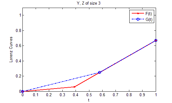
Figure 1: Lorenz curves for BISO channels with the same capacity and output of size 3.

Remark 2.

Not all BISO channels with the same capacity are more capable comparable. A counter example is the following: Consider a BISO channel $X\to(Y,Z)$ with transition probabilities according to:

$${\rm P}(Y=i|X=0) =a_{i},-2\leq i\leq 2$$

$${\rm P}(Z=j|X=0) =b_{j},-2\leq j\leq 2$$

where $a_{-2}=0.061,a_{-1}=a_{1}=\frac{1-10a_{-2}}{2},a_{2}=9a_{-2}$ and $b_{-2}=0.0634977,b_{-1}=\frac{1-b_{-2}}{5},b_{1}=\frac{4(1-b_{-2})}{5},b_{2}=0.$ One can verify that the channels have same capacity, but are not more capable comparable.

2.1.3 On more capable and essentially less noisy orderings in BISO channels

In this section we will establish that these two partial orderings, restricted to $\mathcal{C}$, are inverses of each other(!). This is counter-intuitive as more capable and essentially less noisy are two notions of saying that one receiver is superior to another receiver.

Below (for a complete argument see Lemma 1 in [7]) we note that the uniform input distribution forms a sufficient class for a broadcast channel consisting of two channels $F_{1},F_{2}\in{\cal C}$.

Claim 1.

Consider a binary input broadcast channel whose component channels, $F_{1}:X\to Y_{1}$ and $F_{2}:X\to Y_{2}$ are both output-symmetric, i.e. $F_{1},F_{2}\in{\cal C}$. Then the uniform input distribution ${\rm P}(X=0)=\frac{1}{2}$ forms a sufficient class.

Proof.

The following construction suffices - we leave the details to the reader. Let $j,k\in\{0,1\}$; then define

$$\textrm{Q}(U=(u,j),V=(v,k),X=x)=\begin{cases}\begin{array}[]{ll}\frac{1}{2}\textrm{P}(U=u,V=v,X=x\oplus j)&j=k\\ 0&j\neq k\end{array}\end{cases}.$$

∎

Lemma 4.

Let $F_{1},F_{2}\in{\cal C}(C)$; then $F_{1}\gg F_{2}\iff F_{2}\succeq F_{1}$.

Proof.

Assume $F_{1}\gg F_{2}$. From Claim 1 we know that ${\rm P}(X=0)=\frac{1}{2}$ is a sufficient distribution for the channels $F_{1},F_{2}$. Therefore, when ${\rm P}(X=0)=\frac{1}{2}$ we have for all $U$ such that $U\to X\to(Y_{1},Y_{2})$

$$I(U;Y_{1}) =I(X;Y_{1})-I(X;Y_{1}|U)$$

$$=C-I(X;Y_{1}|U)$$

$$=I(X;Y_{2})-I(X;Y_{1}|U)$$

$$=I(U;Y_{2})+I(X;Y_{2}|U)-I(X;Y_{1}|U)$$

$$\leq I(U;Y_{2}),$$

where the last inequality follows from $F_{1}\gg F_{2}$. Since ${\rm P}(X=0)=\frac{1}{2}$ is a sufficient class of input distributions for a broadcast channel comprising of $F_{1},F_{2}$ it follows from the definition that $F_{2}\succeq F_{1}$.

Assume $F_{2}\succeq F_{1}$. The proof follows by contradiction. Suppose there is a value $x$ such that when ${\rm P}(X=0)=x,I(X;Y_{2})-I(X;Y_{1})=\delta>0$, then consider a $U$ such that ${\rm P}(U=0)={\rm P}(U=1)=\frac{1}{2}$, ${\rm P}(X=0|U=0)=x={\rm P}(X=1|U=1)$. Observe that, from the symmetry $I(X;Y_{2}|U)-I(X;Y_{1}|U)=\delta>0$. However since ${\rm P}(X=0)=\frac{1}{2}$, using a similar decomposition we see that

$$I(U;Y_{1}) =I(U;Y_{2})+I(X;Y_{2}|U)-I(X;Y_{1}|U)$$

$$=I(U;Y_{2})+\delta>I(U;Y_{2}),$$

contradicting the assumption $F_{2}\succeq F_{1}$. Therefore $F_{1}\gg F_{2}$. ∎

The following lemma is an immediate consequence of Corollaries 1, 2, and Lemma 4.

Lemma 5.

Let $BSC(C)$ represent a binary symmetric channel with capacity $C$, $BEC(C)$ - a binary erasure channel with capacity $C$, and $F(C)$ - an arbitrary binary input symmetric output channel, i.e. $F\in{\cal C}$, with capacity $C$. We have

• $BEC(C)\gg F(C)\gg BSC(C)$,

• $BSC(C)\succeq F(C)\succeq BEC(C)$.

This leads us to one of the main results in this paper.

Theorem 2.

Let $BSC(C)$ represent a binary symmetric channel with capacity $C$, $BEC(C)$ - a binary erasure channel with capacity $C$, and $F(C)$ - an arbitrary binary input symmetric output channel, i.e. $F\in{\cal C}$, with capacity $C$. For any three numbers $0\leq C_{1}\leq C_{2}\leq C_{3}$ we have

• $BEC(C_{3})\gg F(C_{2})\gg BSC(C_{1})$,

• $BSC(C_{3})\succeq F(C_{2})\succeq BEC(C_{1})$.

Proof.

If $C_{a}<C_{b}$ then $BSC(C_{a}),BEC(C_{a})$ are degraded versions of $BSC(C_{b}),BEC(C_{b})$ respectively. Hence from Lemma 5 we have

$$BEC(C_{3})\gg BEC(C_{2})\gg F(C_{2})\gg BSC(C_{2})\gg BSC(C_{1}),$$

$$BSC(C_{3})\succeq BSC(C_{2})\succeq F(C_{2})\succeq BEC(C_{2})\succeq BEC(C_{1}).$$

∎

The following corollary is immediate.

Corollary 4.

Superposition coding region is the capacity region for a BISO-broadcast channel if any one of the channels is either a BSC or a BEC.

Proof.

Superposition coding is optimal both for more capable comparable channels[2] and for essentially less noisy comparable channels [7]. From Theorem 2, if any one of the channels is either a BSC or a BEC, then the channels are either more capable comparable or essentially less noisy comparable. ∎

Remark 3.

In [7] the capacity region of a BSC/BEC broadcast channel was established. Corollary 4 generalizes this result to only requiring that one of the BISO channels is a BEC or a BSC.

2.2 Comparison of inner and outer bounds for BISO channels

The following are some commonly used inner bounds (or achievable rate regions) for the capacity region (CR):

• Time-Division region (TD): This region is characterized by the set of points

  $$R_{1} \leq\alpha C_{1}$$

  $$R_{2} \leq(1-\alpha)C_{2},$$

  where $C_{1}$ and $C_{2}$ are the channel capacities for the two receivers, respectively. The rates are achieved by transmitting at capacity $C_{1}$ to the first receiver for fraction $\alpha$ of the time, and at capacity $C_{2}$ to second receiver for the remaining fraction.

• Randomized Time-Divison region (RTD): This corresponds to a time-division strategy except that the slots for which communication occurs to one receiver is also drawn from a codebook which conveys additional information. The rates are characterized by

  $$R_{1} \leq I(W;Y_{1})+{\rm P}(W=0)I(X;Y_{1}|W=0)$$

  $$R_{2} \leq I(W;Y_{2})+{\rm P}(W=1)I(X;Y_{2}|W=1)$$

  $$R_{1}+R_{2} \leq\min\{I(W;Y_{1}),I(W;Y_{2})\}+{\rm P}(W=0)I(X;Y_{1}|W=0)+{\rm P}(W=1)I(X;Y_{2}|W=1),$$

  over binary random variables $W$ satisfying $W\to X\to(Y_{1},Y_{2})$ being Markov. The binary random variable $W$ characterizes the slots which distinguish communication to one receiver over the other.

• Marton’s Inner bound (MIB): This is the best known achievable rate region. The rates are characterized by

  $$R_{1} \leq I(U,W;Y_{1})$$

  $$R_{2} \leq I(V,W;Y_{2})$$

  $$R_{1}+R_{2} \leq\min\{I(W;Y_{1}),I(W;Y_{2})\}+I(U;Y_{1}|W)+I(V;Y_{2}|W)-I(U;V|W),$$

  over random variables $(U,V,W)$ satisfying $(U,V,W)\to X\to(Y_{1},Y_{2})$ being Markov. Observe that setting $U=X,V=\emptyset$ when $W=0$ and $V=X,U=\emptyset$ when $W=1$ reduces MIB to the RTD region.

  Lemma 6 ([8]).

  For binary input broadcast channels, the maximum sum rate implied by Marton’s inner bound(MIB) matches that of randomized time-divison(RTD) region.

• Outer bound (OB): The following region[6] represents an outer bound to the capacity region. The union of rate pairs

  $$R_{1} \leq I(U;Y_{1})$$

  $$R_{2} \leq I(V;Y_{2})$$

  $$R_{1}+R_{2} \leq I(U;Y_{1})+I(X;Y_{2}|U)$$

  $$R_{1}+R_{2} \leq I(V;Y_{2})+I(X;Y_{1}|V)$$

  over all $(U,V)\to X\to(Y_{1},Y_{2})$ represents an outer bound to the capacity region.

  Remark 4.

  For BISO channels since ${\rm P}(X=0)=\frac{1}{2}$ is a common sufficient distribution, it can be shown that the OB matches an earlier outer bound due to Körner and Marton [5].

We adopt the notation in Table 1.

Table 1: Notation

Abbr.		Abbr.
TD	time-division region	BSC	binary symmetric channel
RTD	randomized time-division region	BEC	binary erasure channel
MIB	Marton’s inner bound	e.l.n.	essentially less noisy
CR	capacity region	e.m.c.	essentially more capable
OB	Outer bound (Körner-Marton, Nair-El Gamal)	$*$	binary convolution
BISO	binary input symmetric output	$h(\cdot)$	binary entropy function

Lemma 7.

Consider a 2-receiver broadcast channel where both $X\to Y_{1}$ and $X\to Y_{2}$ represent the BISO channels with transition probabilities $\{q_{k},q_{-k}:1\leq k\leq N\}$ and $\{p_{j},p_{-j}:1\leq j\leq N\}$ respectively. Consider the following region formed by taking the union of rate pairs $(R_{1},R_{2})$ satisfying

$$R_{2} \leq I(U;Y_{2})$$

$$R_{2}+R_{1} \leq I(U;Y_{2})+I(X;Y_{1}|U)$$

$$R_{1} \leq I(X;Y_{1})$$

over all $p(u)p(x|u)p(y_{1},y_{2}|x)$. Then the same region can be realized by restricting to a binary $U$ such that $U\to X\sim BSC(s)$ and ${\rm P}(X=0)=\frac{1}{2}$.

Proof.

The proof is presented in the Appendix. ∎

Let $U\to X\sim BSC(s_{1}),V\to X\sim BSC(s_{2})$ and ${\rm P}(X=0)=\frac{1}{2}$. Let $I(U;Y_{1})=f_{1}(s_{1})$, where ${\rm P}(X=1|U=0)=s_{1}$, and define $I(V;Y_{2})=f_{2}(s_{2})$ in a similar fashion. It is clear from symmetry that $f_{1}(s)=f_{1}(1-s),f_{2}(s)=f_{2}(1-s).$

From Lemma 7 and Remark 4 it follows that OB can be written as the union of rate pairs $R_{1},R_{2}$ satisfying

$$R_{1} \leq f_{1}(s_{1})$$

$$R_{2} \leq f_{2}(s_{2})$$

$$R_{1}+R_{2} \leq f_{1}(s_{1})+C-f_{2}(s_{1})$$ (3)

$$R_{1}+R_{2} \leq f_{2}(s_{2})+C-f_{1}(s_{2}).$$

for some $0\leq s_{1},s_{2}\leq\frac{1}{2}$.

Let

$$I =\{s\in[0,0.5]:f_{1}(s)>f_{2}(s)\}$$

$$J =\{s\in[0,0.5]:f_{1}(s)<f_{2}(s)\}.$$

The following result relates the equivalence of the various bounds and their relation to whether the channels are more capable comparable.

Theorem 3.

Let $F_{1},F_{2}\in\mathcal{C}(C)$. Then the following are equivalent:

1. $F_{1}$ and $F_{2}$ are not more capable comparable

2. $TD\subset OB$

3. There exists $s_{1}\in I,s_{2}\in J$ such that $f_{1}(s_{1})+f_{2}(s_{2})>C$

4. $TD\subset MIB$

5. $MIB\subset OB$.

Proof.

The proof of this equivalence is presented in the Appendix. ∎

Corollary 5.

For two BISO channels with the same capacity, superposition coding is optimal if and only if the channels are more capable comparable.

Proof.

If superposition coding region is indeed the capacity region, then we have $R_{1}+R_{2}\leq I(X;Y_{1})\leq C$. Further since the two channels have the same capacity, we have the TD region is optimal. From Theorem 3 we have that the channels are more capable comparable. ∎

Remark 5.

A characterization of when superposition coding is optimal for 2-receiver broadcast channels is open in general. It is known that superposition coding is optimal when the channels are either essentially more capable comparable or essentially less noisy comparable[7] - two incompatible notions. However a converse statement is still unknown.

Observation 1.

From remark 2 we know that there exists a pair of channels $F_{1},F_{2}\in\mathcal{C}(C)$ which are not more capable comparable. Hence from Theorem 3 we know that the capacity region is strictly larger than TD. However, if we replace $F_{2}$ by $BEC(C)$, a more capable channel, then the capacity of the broadcast channel formed by $F_{1}$ and $BEC(C)$ is the TD region (Corollary 2). Thus replacing by a more capable channel can strictly reduce the capacity region.

This observation leads to an operational definition of a better receiver and a partial order as follows.

2.2.1 A new partial order

We now introduce a natural operational partial order among broadcast channels.

Definition 7.

Receiver $Z_{2}$ is a better receiver than $Y_{2}$ if the capacity region of $X\to(Y_{1},Z_{2})$ contains that of $X\to(Y_{1},Y_{2})$ for every channel $X\to Y_{1}$. In other words, if we replace receiver $Y_{2}$ by receiver $Z_{2}$ then the capacity region will not decrease.

Remark 6.

Note that the capacity region of a broadcast channel just depends on the marginal distributions $X\to Y_{1}$, $X\to Y_{2}$, and hence the definition makes sense.

From Observation 1 we know that a more capable receiver is not necessarily a better receiver. However we will show that if $Z_{2}$ is a less noisy receiver than $Y_{2}$, then $Z_{2}$ is indeed a better receiver than $Y_{2}$.

Claim 2.

If $Z_{2}$ is a less noisy receiver than $Y_{2}$, then $Z_{2}$ is a better receiver than $Y_{2}$.

Proof.

The capacity region of a discrete memoryless broadcast channel has the following $n$-letter characterization. Consider the region $\mathcal{R}_{n}$ defined as the union of rate pairs $(R_{1},R_{2})$ that satisfy

$$R_{1}\leq\frac{1}{n}I(U;Y_{1}^{n})$$

$$R_{2}\leq\frac{1}{n}I(V;Y_{2}^{n})$$

for some $p(u)p(v)p(x^{n}|u,v)$. It is known that the capacity region is $\lim_{n}\mathcal{R}_{n}$. (This is folklore. It is clear that this is achievable, and a converse follows by setting $U=M_{1}$ and $V=M_{2}$ and applying Fano’s inequality.) Observe that

$$I(V;Y_{2,1}^{~{}j},Z_{2,j+1}^{~{}n}) =I(V;Y_{2,1}^{j-1},Z_{2,j+1}^{~{}n})+I(V;Y_{2j}|Y_{2,1}^{j-1},Z_{2,j+1}^{~{}n}),~{}j=n,\ldots,1$$

$$\leq I(V;Y_{2,1}^{j-1},Z_{2,j+1}^{~{}n})+I(V;Z_{2j}|Y_{2,1}^{j-1},Z_{2,j+1}^{~{}n})$$

$$=I(V;Y_{2,1}^{j-1},Z_{2,j}^{~{}n}).$$

By taking the extreme points of this chain we obtain that $I(V;Y_{2}^{n})\leq I(V;Z_{2}^{n})$. Claim follows from the expression of the capacity region stated above. ∎

3 Conclusion

We look at partial orders induced by the more capable relations and less noisy relations in binary-input symmetric-output(BISO) broadcast channels. We establish the capacity regions for a class of them and also show various other results related to the evaluation of various bounds. Some of the results act contrary to popular intuition and hence BISO channels can serve as a simple class from which we can improve our understanding of various relations. We also use perturbation based arguments to show the optimality of certain auxiliary channels, thus generalizing earlier results. We hope that some of the results presented here can invoke a careful rethinking of various notions of dominance between receivers.

Appendix

A.1 Proof to Lemma 7

Proof.

Let ${\cal U}=\{1,2,...,m\}$, ${\rm P}(U=i)=u_{i}$ and ${\rm P}(X=0|U=i)=s_{i}$. Further let $h(x)=-x\log_{2}x-(1-x)\log_{2}(1-x)$ be the binary entropy function and let $*$ denote the binary convolution, i.e. $a*b=a(1-b)+b(1-a)$.

Using these notations we have the following expansions,

$$I(U;Y_{2}) =\sum_{j}(p_{j}+p_{-j})\big{(}h(\frac{p_{j}}{p_{j}+p_{-j}}*\sum_{i}u_{i}s_{i})-\sum_{i}u_{i}h(\frac{p_{j}}{p_{j}+p_{-j}}*s_{i})\big{)}$$

$$I(X;Y_{1}|U) =\sum_{k}(q_{k}+q_{-k})\big{(}\sum_{i}u_{i}h(\frac{q_{k}}{q_{k}+q_{-k}}*s_{i})-h(\frac{q_{k}}{q_{k}+q_{-k}})\big{)}$$

$$I(X;Y_{1}) =\sum_{k}(q_{k}+q_{-k})\big{(}h(\frac{q_{k}}{q_{k}+q_{-k}}*\sum_{i}u_{i}s_{i})-h(\frac{q_{k}}{q_{k}+q_{-k}})\big{)}.$$

Define $\tilde{{\cal U}}=\{1,2,...,m\}\times\{1,2\}$, ${\rm P}(\tilde{U}=(i,1))=\frac{u_{i}}{2}$, ${\rm P}(X=0|\tilde{U}=(i,1))=s_{i}$, ${\rm P}(\tilde{U}=(i,2))=\frac{u_{i}}{2}$, and ${\rm P}(X=0|\tilde{U}=(i,2))=1-s_{i}$. This induces an $\tilde{X}$ with ${\rm P}(\tilde{X}=0)=\frac{1}{2}$ and it is straightforward to notice

$$I(\tilde{U};\tilde{Y}_{2}) \geq I(U;Y_{2}),$$

$$I(\tilde{X};\tilde{Y}_{1}|\tilde{U}) =I(X;Y_{1}|U),$$

$$I(\tilde{X};\tilde{Y}_{1}) \geq I(X;Y_{1}).$$

Thus for every $U$ replacing $U$ by $\tilde{U}$ leads to a larger achievable region.

Hence it suffices to maximize over all auxiliary random variables of the form $(U,X)$ defined by: ${\cal U}=\{1,2,...,m\}\times\{1,2\}$, ${\rm P}(U=(i,1))=\frac{u_{i}}{2}$, ${\rm P}(X=0|U=(i,1))=s_{i}$, ${\rm P}(U=(i,2))=\frac{u_{i}}{2}$ and ${\rm P}(X=0|U=(i,2))=1-s_{i}$. Let this class of random variables $(U,X)$ be $\mathcal{Q}$.

Since ${\rm P}(X=0)=\frac{1}{2}$ remains fixed, the third inequality remains constant. Therefore, to compute the extreme points, we proceed to compute the distribution $(U,X)$ (belonging to $\mathcal{Q}$) that maximizes $\lambda I(U;Y_{2})+\big{(}I(U;Y_{2})+I(X;Y_{1}|U)\big{)}.$

For a given $p(u,x)\in\mathcal{Q},|\mathcal{U}|=2m$ , consider the multiplicative Lyapunov perturbation defined by

$$R(U=(i,1),X=0) ={\rm P}(U=(i,1),X=0)(1+\varepsilon L(i))$$

$$R(U=(i,1),X=1) ={\rm P}(U=(i,1),X=1)(1+\varepsilon L(i))$$ (4)

$$R(U=(i,2),X=0) =R(U=(i,1),X=1)$$

$$R(U=(i,2),X=1) =R(U=(i,1),X=0)$$

For $r(u,x)$ to be a valid probability distribution we require the conditions $1+\varepsilon L(i)\geq 0,\forall i$ and $\sum_{=1}^{m}i{\rm P}\big{(}U=(i,1)\big{)}L(i)=0.$

Observe that the perturbation maintains ${\rm P}(X=0)$ and further the new pair $r(u,x)$ also belongs to $\mathcal{Q}$. A non-trivial $L$ exists if $m=\frac{|\mathcal{U}|}{2}\geq 2$.

Observe that

$$(\lambda+1)I_{r}(U;Y_{2})+I_{r}(X;Y_{1}|U)$$

$$\quad=(\lambda+1)H_{p}(Y_{2})+\lambda H_{p}(U)+H_{p}(U,Y_{1})-(\lambda+1)H_{p}(U,Y_{2})$$

$$\qquad+\varepsilon\big{(}\lambda H^{L}_{p}(U)+H^{L}_{p}(U,Y_{1})-(\lambda+1)H^{L}_{p}(U,Y_{2})\big{)}$$

where

$$H^{L}_{p}(U) =-\sum_{i}2p(i)L(i)\log 2p(i)$$

$$H^{L}_{p}(U,Y_{1}) =-\sum_{i,y_{1}}2p(i,y_{1})L(i)\log 2p(i,y_{1})$$

$$H^{L}_{p}(U,Y_{2}) =-\sum_{i,y_{2}}2p(i,y_{2})L(i)\log 2p(i,y_{2}).$$

The first derivative with respect to $\varepsilon$ being zero implies

$$\lambda H^{L}_{p}(U)+H^{L}_{p}(U,Y_{1})-(\lambda+1)H^{L}_{p}(U,Y_{2})=0$$

and this further implies that if $p(u,x)$ achieves the maximum of $(\lambda+1)I_{p}(U;Y_{2})+I_{p}(X;Y_{1}|U)$ then $(\lambda+1)I_{r}(U;Y_{2})+I_{r}(X;Y_{1}|U)=(\lambda+1)I_{p}(U;Y_{2})+I_{p}(X;Y_{1}|U)$ for any valid perturbation that satisfies (4).

Now we choose $\varepsilon$ such that $\min_{i}1+\varepsilon L(i)=0$, and let $i=i^{*}$ achieve this minimum. Observe that $r(i^{*})=0$ and hence there exists an $U$ with cardinality equal to $2(m-1)$ such that $(\lambda+1)I(U;Y_{2})+I(X;Y_{1}|U)$ is constant. We can proceed by induction until $m=1$.

Since $(U,X)\in\mathcal{Q}$ and $|\mathcal{U}|=2$, implies that the optimal auxiliary channel $U\to X$ follows the distribution given by

$${\rm P}(U=1) ={\rm P}(U=2)=\frac{1}{2}$$

$${\rm P}(X=0|U=1) ={\rm P}(X=1|U=2)=s,$$

i.e. $U\to X\sim BSC(s)$. ∎

The same proof can also be used to establish the following lemma.

Lemma 8.

Consider a 2-receiver broadcast channels where both $X\to Y_{1}$ and $X\to Y_{2}$ represent the BISO channels with transition probabilities $\{q_{k},q_{-k}:1\leq k\leq N\}$ and $\{p_{j},p_{-j}:1\leq j\leq N\}$ respectively. Consider the following superposition coding region formed by taking the union of rate pairs $(R_{1},R_{2})$ satisfying

$$R_{2} \leq I(U;Y_{2})$$

$$R_{2}+R_{1} \leq I(U;Y_{2})+I(X;Y_{1}|U)$$

$$R_{2}+R_{1} \leq I(X;Y_{1})$$

over all $p(u)p(x|u)p(y_{1},y_{2}|x)$. Then the same region can be realized by restricting to a binary $U$ such that $U\to X\sim BSC(s)$ and ${\rm P}(X=0)=\frac{1}{2}$.

Remark 7.

This generalizes the result by Wyner and Ziv [10] for BSC broadcast channels. In [2] it was shown that superposition coding is indeed optimal when the two channels are more capable comparable.

A.2 Proof to Theorem 3

Proof.

(a) $\Rightarrow$ (b): Recalling: Let

$$I =\{s\in[0,0.5]:f_{1}(s)>f_{2}(s)\}$$

$$J =\{s\in[0,0.5]:f_{1}(s)<f_{2}(s)\}.$$

Since the channels are not more-capable comparable, we know that there esists $s_{1}\in I$ and $s_{2}\in J$. Construct $\tilde{U}\to X$, where $\tilde{U}=U^{\prime}\times Q$ with binary $U^{\prime}$ and $Q$, and probabilities

$${\rm P}(\tilde{U}=(0,0)) =\frac{1-\varepsilon}{2} {\rm P}(X=0|\tilde{U}=(0,0)) =1$$

$${\rm P}(\tilde{U}=(0,1)) =\frac{\varepsilon}{2} {\rm P}(X=0|\tilde{U}=(0,1)) =s_{1}$$

$${\rm P}(\tilde{U}=(1,0)) =\frac{1-\varepsilon}{2} {\rm P}(X=1|\tilde{U}=(1,0)) =1$$

$${\rm P}(\tilde{U}=(1,1)) =\frac{\varepsilon}{2} {\rm P}(X=1|\tilde{U}=(1,1)) =s_{1}.$$

Thus, $U^{\prime}\mapsto X\sim BSC(0)$ conditioned on the event $Q=0$, $U^{\prime}\mapsto X\sim BSC(1-s_{1})$ conditioned on $Q=1$, and further $U^{\prime}$ is independent of $Q$ with ${\rm P}(U^{\prime}=0)=\frac{1}{2}$. We can see that $Q$ is independent of $X$ and hence of $Y_{1},Y_{2}$; thus $I(Q;Y_{1})=I(Q;Y_{2})=0$. Now

$$I(\tilde{U};Y_{1}) =I(U^{\prime},Q;Y_{1})=I(U^{\prime};Y_{1}|Q)+I(Q;Y_{1})$$

$$=I(U^{\prime};Y_{1}|Q)$$

$$=(1-\varepsilon)I(X;Y_{1})+\varepsilon I(U^{\prime};Y_{1}|Q=1)$$

$$=(1-\varepsilon)C+\varepsilon f_{1}(s_{1}).$$

Similarly, we obtain

$$I(\tilde{U};Y_{2})=(1-\varepsilon)C+\varepsilon f_{2}(s_{1}).$$

Thus we have

$$R_{1} \leq(1-\varepsilon)C+\varepsilon f_{1}(s_{1})$$

$$R_{2} \leq f_{2}(s_{2})$$

$$R_{1}+R_{2} \leq I(\tilde{U};Y_{1})+I(X;Y_{2}|\tilde{U})$$

$$=I(\tilde{U};Y_{1})+I(X;Y_{2})-I(\tilde{U};Y_{2})$$

$$=(1-\varepsilon)C+\varepsilon f_{1}(s_{1})+C-[(1-\varepsilon)C+\varepsilon f_{2}(s_{1})]$$

$$=C+\varepsilon[f_{1}(s_{1})-f_{2}(s_{1})]\quad\quad(>C)$$

$$R_{1}+R_{2} \leq I(V;Y_{2})+I(X;Y_{1}|V)$$

$$=f_{2}(s_{2})+C-f_{1}(s_{2})\quad\qquad(>C).$$

To show that we can have $(1-\varepsilon)C+\varepsilon f_{1}(s_{1})+f_{2}(s_{2})>C$, we just need to choose small $\varepsilon$ to ensure $f_{2}(s_{2})>\varepsilon[C-f_{1}(s_{1})]$. Since this is clearly possibe, we have $OB\supset TD$.

(b) $\Rightarrow$ (c): From Equation (3), we have the following expression of the boundary of the outer bound,

$$R_{1} \leq I(U;Y_{1})=f_{1}(s_{1})$$

$$R_{2} \leq I(V;Y_{2})=f_{2}(s_{2})$$

$$R_{1}+R_{2} \leq I(U;Y_{1})+I(X;Y_{2}|U)=f_{1}(s_{1})+C-f_{2}(s_{1})$$

$$R_{1}+R_{2} \leq I(V;Y_{2})+I(X;Y_{1}|V)=f_{2}(s_{2})+C-f_{1}(s_{2})$$

Clearly for every $s_{1}\in I,s_{2}\in J$ if $f_{1}(s_{1})+f_{2}(s_{2})\leq C$ then from above $OB=TD$. However since $OB\supset TD$, there exists $s_{1}\in I,s_{2}\in J$ such that $f_{1}(s_{1})+f_{2}(s_{2})>C$.

(c) $\Rightarrow$ (d): In general, $TD\subseteq RTD\subseteq MIB$. So now it suffices to show there exists an example where the sum rate of RTD region is strictly larger than TD region.

We now compute the maximum sum rate of the RTD region. From Lemma 6 we know that this matches the maximum sum rate of the MIB region.

Consider an auxiliary channel $W\to X$ such that

$${\rm P}(W=0)=a,\quad {\rm P}(W=1)=1-a$$

$${\rm P}(X=0|W=0)=s_{2},\quad {\rm P}(X=0|W=1)=s_{1}$$

where $as_{2}+(1-a)s_{1}=\frac{1}{2}$.

It is straightforward to check the following

$$I(X;Y_{1}|W=0)=C-f_{1}(s_{2}),~{}I(X;Y_{1}|W=1)=C-f_{1}(s_{1})$$

$$I(X;Y_{2}|W=0)=C-f_{2}(s_{2}),~{}I(X;Y_{2}|W=1)=C-f_{2}(s_{1}),$$

$$I(X;Y_{1})=I(X;Y_{2})=C.$$

Then observe that

$$I(W;Y_{1})+{\rm P}(W=0)I(X;Y_{1}|W=0)+{\rm P}(W=1)I(X;Y_{2}|W=1)$$

$$\quad=I(X;Y_{1})+{\rm P}(W=1)\big{(}I(X;Y_{2}|W=1)-I(X;Y_{1}|W=1)\big{)}$$

$$\quad=C+(1-a)(f_{1}(s_{1})-f_{2}(s_{1}))$$

where the last inequality holds since $s_{1}\in I$.

Similarly

$$I(W;Y_{2})+{\rm P}(W=0)I(X;Y_{1}|W=0)+{\rm P}(W=1)I(X;Y_{2}|W=1)=C+a(f_{2}(s_{2})-f_{1}(s_{2})).$$

Therefore the sum rate of RTD (eq. MIB) for this choice of $(W,X)$ is given by

$$C+\min\{(1-a)(f_{1}(s_{1})-f_{2}(s_{1})),a(f_{2}(s_{2})-f_{1}(s_{2}))\}.$$ (5)

Therefore if $(c)$ is satisfied, i.e. there exists $s_{1}\in I,s_{2}\in J$, then there exists a $(W,X)$ so that equation (5) gives a sum rate strictly larger than $C$.

Remark 8.

A careful reader will notice that the above argument only requires $s_{1}\in I,s_{2}\in J$ and does not even require $f_{1}(s_{1})+f_{2}(s_{2})>C$. But existence of any $s_{a}\in I,s_{b}\in J$ will imply that $(a)$ holds and hence $(c)$ holds.

(d) $\Rightarrow$ (e): Since $TD\subset MIB$, to compute the maximum sum rate of MIB it suffices to maximize over $s_{1}\in I,s_{2}\in J,0<a<1$ the term

$$C+\min\{(1-a)(f_{1}(s_{1})-f_{2}(s_{1})),a(f_{2}(s_{2})-f_{1}(s_{2}))\}.$$

Consider any triple $s_{1}\in I,s_{2}\in J,0<a<1$. Pick any $\varepsilon>0$ small enough (will show later how small we require it).

Define $(U,X)=(Q,U_{1},X)$ where ${\rm P}(Q=0)=1-a+\varepsilon,{\rm P}(Q=1)=a-\varepsilon$; and $U_{1}\mapsto X\sim BSC(s_{1})$ conditioned on $Q=0$, and $U_{1}\mapsto X\sim BSC(0)$ conditioned on $Q=1$. Further take ${\rm P}(U_{1}=0)={\rm P}(U_{1}=1)=\frac{1}{2}$. Observe that this induces ${\rm P}(X=0)={\rm P}(X=1)=\frac{1}{2}$.

Similarly define $(V,X)=(Q^{\prime},V_{1},X)$ where ${\rm P}(Q^{\prime}=0)=a+\varepsilon,{\rm P}(Q^{\prime}=1)=1-a-\varepsilon$; and $V_{1}\mapsto X\sim BSC(s_{2})$ conditioned on $Q^{\prime}=0$, and $V_{1}\mapsto X\sim BSC(0)$ conditioned on $Q^{\prime}=1$. Further take ${\rm P}(V_{1}=0)={\rm P}(V_{1}=1)=\frac{1}{2}$. Observe that this also induces ${\rm P}(X=0)={\rm P}(X=1)=\frac{1}{2}$.

Since the distribution of $X$ is consistent there exists a triple $(U,V,X)$ with the same pairwise marginals $(U,X)$ and $(V,X)$ as described earlier. With this choice, OB reduces to

$$R_{1} \leq I(U;Y_{1})=(1-a+\varepsilon)f_{1}(s_{1})+(a-\varepsilon)C$$

$$R_{2} \leq I(V;Y_{2})=(a+\varepsilon)f_{2}(s_{2})+(1-a-\varepsilon)C$$

$$R_{1}+R_{2} \leq I(U;Y_{1})+I(X;Y_{2}|U)=C+(1-a+\varepsilon)(f_{1}(s_{1})-f_{2}(s_{1}))$$

$$R_{1}+R_{2} \leq I(V;Y_{2})+I(X;Y_{1}|V)=C+(a+\varepsilon)(f_{2}(s_{2})-f_{1}(s_{2})).$$

Clearly the maximum sum rate of the above region is minimum of the terms

$$\{C+(1-a+\varepsilon)(f_{1}(s_{1})-f_{2}(s_{1})),C+(a+\varepsilon)(f_{2}(s_{2})-f_{1}(s_{2})),(1-2\epsilon)C+(1-a+\varepsilon)f_{1}(s_{1})+(a+\varepsilon)f_{2}(s_{2})\}.$$

We pick $\varepsilon>0$ to satisfy

$$(1-2\epsilon)C+(1-a+\varepsilon)f_{1}(s_{1})+(a+\varepsilon)f_{2}(s_{2})>C+(1-a)(f_{1}(s_{1})-f_{2}(s_{1}))$$

$$\Leftrightarrow\quad (1-a)f_{2}(s_{1})+af_{2}(s_{2})>\varepsilon(2C-f_{1}(s_{1})-f_{2}(s_{2})),$$

and

$$af_{1}(s_{2})+(1-a)f_{2}(s_{1})>\varepsilon(2C-f_{1}(s_{1})-f_{2}(s_{2})),$$

then the maximum sum rate of the OB expression will be strictly bigger than that of MIB region. Since this is possible for every $s_{1}\in I,s_{2}\in J,0<a<1$, the maximum sum rate of OB is strictly larger than that of MIB. Therefore $OB\supset MIB$ or $(e)$ holds.

(e) $\Rightarrow$ (a): Since $MIB\subset OB$ clearly implies the channels are not more capable comparable. This is because when the channels are more capable comparable we know from [2] that superposition coding is optimal and that $MIB=CR=OB$. ∎

References

• [1] T Cover, Broadcast channels, IEEE Trans. Info. Theory IT-18 (January, 1972), 2–14.
• [2] A El Gamal, The capacity of a class of broadcast channels, IEEE Trans. Info. Theory IT-25 (March, 1979), 166–169.
• [3] B Hajek and M Pursley, Evaluation of an achievable rate region for the broadcast channel, IEEE Trans. Info. Theory IT-25 (January, 1979), 36–46.
• [4] J Körner and K Marton, Comparison of two noisy channels, Topics in Inform. Theory(ed. by I. Csiszar and P.Elias), Keszthely, Hungary (August, 1975), 411–423.
• [5] K Marton, A coding theorem for the discrete memoryless broadcast channel, IEEE Trans. Info. Theory IT-25 (May, 1979), 306–311.
• [6] C Nair and A El Gamal, An outer bound to the capacity region of the broadcast channel, IEEE Trans. Info. Theory IT-53 (January, 2007), 350–355.
• [7] Chandra Nair, Capacity regions of two new classes of 2-receiver broadcast channels, International Symposium on Information Theory (2009), 1839–1843.
• [8] Chandra Nair, Zizhou Vincent Wang, and Yanlin Geng, An information inequality and evaluation of marton’s inner bound for binary input broadcast channels, CoRR abs/1001.1468 (2010).
• [9] I. Sutskover, S. Shamai, and J. Ziv, Extremes of information combining, Information Theory, IEEE Transactions on 51 (2005), no. 4, 1313–1325.
• [10] A. Wyner and J. Ziv, A theorem on the entropy of certain binary sequences and applications: Part I, IEEE Trans. Inform. Theory IT-19 (1973), no. 6, 769–772.