Abstract

We investigate the linear propagation of a paraxial optical beam in anisotropic media. We start from the eigenmode solution of the plane wave in the media, then subsequently derive the wave equation for the beam propagating along a general direction except the optic axes. The wave equation has a term containing the second mixed partial derivative which originates from the anisotropy, and this term can result in the rotation of the beam spot. The rotation effect is investigated by solving analytically the wave equation with an initial elliptical Gaussian beam for both uniaxial and biaxial media. For both media, it is found that there exists a specific direction, which is dependent on anisotropy of the media, on the cross-section perpendicular to propagation direction to determine the rotation of the beam spot. When the major axis of the elliptical spot of the input beam is parallel to or perpendicular to the specific direction, the beam spot will not rotate during propagation, otherwise, it will rotate with the direction and the velocity determined by input parameters of the beam.

OCIS codes: 260.1180, 260.1960.

1 Introduction

The propagation of light in anisotropic media is still receiving a good deal of attention from both the experimental and the theoretical points of view. The subject is of fundamental interest because of its important role in polarizers, compensators, amplitude- and phase-modulation devices, also, in nonlinear optical phenomena which usually take place in anisotropic media. An accurate electromagnetic description is required for the evaluation of the field distribution in, for example, designing polarizers and compensators or in describing the nonlinear processes like second harmonic generation.

A number of studies [1, 2, 3, 4, 5, 6, 7, 8, 9, 10, 11, 12] have been devoted to an analysis of optical beam propagation in anisotropic medium, but most of them are concerned about the uniaxial cases. For instance, Fleck et al. [1] derived the paraxial equations for both the ordinary and the extraordinary components of the field in uniform uniaxial anisotropic media. The derivation is based on the paraxial approximation that the electric field corresponding to the beam is plane polarized with a polarization corresponding to either an ordinary or an extraordinary wave. Ciattoni et al. [2, 3, 4, 5, 6] proposed a theoretical scheme that the exact plane wave angular spectrum representation is approximated within the paraxial constraint, obtaining the paraxial expressions for the ordinary and extraordinary components of a field propagating in uniaxial media. Trippenbach et al. [7, 8] considered the propagation of light pulses in anisotropic and dispersive media, deriving the equation for the slowly varying envelope of the electric field. The equation has applications in divers fields. In their paper, it was used to investigate the propagation of an optical pulse in uniaxial media, and found that the equation contains terms that rotate the pulse in time domain. The rotation effect that originate because of the anisotropy of the medium and the finite size of the field. The similar effect in spatial domain can be found in the beam propagation in anisotropic media, however, it remains undiscussed.

Generally speaking, investigation of optical beam propagation in biaxial media is more complicated than that in uniaxial media because of the lower symmetry in the dielectric tensor of the former. To our knowledge, the first attempt to quantify the propagation of beam in biaxial media was made by Dreger [9]. In his paper, he derived the optical beam propagators for biaxial media and specialized them for three cases of wave-vector direction: general directions, coincident with an optic axis, and nearly parallel to an optic axis. His derivation refers to complicated mathematical analysis. In our paper, we will give another way of deriving the wave equation for paraxial beam propagating in the general directions.

The paper is organized as follow: In section 2, we use the method that has been introduced in [13] to obtain the eigenmode solution in biaxial media. This method is well known, but to our knowledge, the results for biaxial media are unavailable in the literatures published so far. In section 3 we derive the equation for the optical beam in anisotropic media. Previously, Qi Guo and Sien Chi [10] have derived the nonlinear paraxial wave equation for the propagation of an optical beam in anisotropic media. Because the nonlinear effect are treated as a small perturbation, the whole derivation is available for the linear situation if the nonlinear term is not considered. Besides, we find that there is an improper approximation in the process of the derivation. In this section, therefore, we adopt their way to derive the beam equation and make an improvement in the derivation. In section 4 we illustrate the dynamics of the beam propagation by using initial elliptical Gaussian beams. Section 5 is a summary.

2 Eigenmodes in anisotropic media

We start from the eigenanalysis of optical field in anisotropic media. From the beginning to Eq. (14) in this section, we briefly recall the principles of the methods of how to obtain the eigenmodes, referring the readers to previous publications for details.

For a monochromatic optical field $\mathbf{E}(\mathbf{r},t)=\mathbf{E}(\mathbf{r})\exp(i\omega t)$ in a magnetically uniform anisotropic medium, $\mathbf{E}(\mathbf{r})$ is described by the wave equation [1]

$$\nabla\times[\nabla\times\mathbf{E}(\mathbf{r})]-\frac{\omega^{2}}{c^{2}}\hat{\varepsilon}\cdot\textbf{E}(\mathbf{r})=0,$$ (1)

where $\hat{\varepsilon}$ is the relative dielectric tensor. Assuming that Eq. (1) has a plane wave solution

$$\mathbf{E}(\mathbf{r})=\mathbf{E}_{0}\exp(-i\mathbf{k}\cdot\mathbf{r}),$$ (2)

where the amplitude $\mathbf{E}_{0}$ is a constant and $\mathbf{k}$ is the wave vector, we have the following eigenvalue equation [14]

$$(\mathbf{k}\mathbf{k}-k^{2}\hat{I}+\frac{\omega^{2}}{c^{2}}\hat{\varepsilon})\cdot\mathbf{E}_{0}=0,$$ (3)

where $\hat{I}$ is an unit tensor of rank 2. Moreover, the dispersion relation

$$\det(\mathbf{k}\mathbf{k}-k^{2}\hat{I}+\frac{\omega^{2}}{c^{2}}\hat{\varepsilon})=0$$ (4)

can be obtained from the necessary condition for nontrivial solutions to Eq. (3). On the other hand, the electric field $\mathbf{E}$ and the electric displacement $\mathbf{D}$ are related by the constitutive law,

$$\mathbf{D}=\varepsilon_{0}\hat{\varepsilon}\cdot\mathbf{E},$$ (5)

where $\varepsilon_{0}$ is the dielectric constant in vacuum. The Gauss’s law for the plane wave requires that

$$\mathbf{k}\cdot\mathbf{D}=0,$$ (6)

implying that $\mathbf{k}$ is perpendicular to $\mathbf{D}$. It is proved [13, 15] that for every direction of propagation $\mathbf{k}/|\mathbf{k}|$ for the plane wave in anisotropic media, there are, in general, two orthogonal polarizations of $\mathbf{D}$ and, correspondingly, two values of $\mathbf{k}$. The allowed plane waves are called eigenmodes and their corresponding polarization directions $\mathbf{D}/|\mathbf{D}|$ are called eigenvectors [15]. As soon as $\mathbf{D}/|\mathbf{D}|$ are found, the polarizations of $\mathbf{E}$ can be obtained from the inverse function of Eq. (5),

$$\frac{\mathbf{E}}{|\mathbf{E}|}=\frac{\hat{\varepsilon}^{-1}\cdot\frac{\mathbf{D}}{|\mathbf{D}|}}{|\hat{\varepsilon}^{-1}\cdot\frac{\mathbf{D}}{|\mathbf{D}|}|},$$ (7)

where $\hat{\varepsilon}^{-1}$ is the inverse of the tenser $\hat{\varepsilon}$. One convenient way of finding $\mathbf{D}/|\mathbf{D}|$ can be visualized with the aid of the index ellipsoid [13], so we are going to solve the eigenmodes problem in biaxial media by this way.

Consider a lossless anisotropic medium, in the principle coordinate system $(x^{\prime},y^{\prime},z^{\prime})$, characterized by primes, the dielectric tensor $\hat{\varepsilon}^{\prime}$ is of a diagonal form,

$$\hat{\varepsilon}^{\prime}=\left(\begin{array}[]{ccc}\varepsilon_{x^{\prime}}&0&0\\ 0&\varepsilon_{y^{\prime}}&0\\ 0&0&\varepsilon_{z^{\prime}}\\ \end{array}\right),$$ (8)

where $\varepsilon_{x^{\prime}}$, $\varepsilon_{y^{\prime}}$ and $\varepsilon_{z^{\prime}}$ are real, and $\varepsilon_{x^{\prime}}>\varepsilon_{y^{\prime}}>\varepsilon_{z^{\prime}}$ is supposed by convenience. The equation of the index ellipsoid is [13]

$$\frac{x^{\prime 2}}{\varepsilon_{x^{\prime}}}+\frac{y^{\prime 2}}{\varepsilon_{y^{\prime}}}+\frac{z^{\prime 2}}{\varepsilon_{z^{\prime}}}=1,$$ (9)

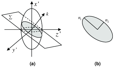
Fig. 1: (a)Index ellipsoid and (b) the ellipse that the plane $\Sigma$ cuts in the index ellipsoid.

as shown in Fig. 1(a). We write the wave vector $\mathbf{k}$ of the plane wave in the form of

$$\mathbf{k}=\mathbf{e_{x^{\prime}}}k_{x^{\prime}}+\mathbf{e_{y^{\prime}}}k_{y^{\prime}}+\mathbf{e_{z^{\prime}}}k_{z^{\prime}},$$ (10)

where $\mathbf{e_{x^{\prime}}}$, $\mathbf{e_{y^{\prime}}}$ and $\mathbf{e_{z^{\prime}}}$ are unit vectors along $x^{\prime}$, $y^{\prime}$ and $z^{\prime}$ axes, respectively, while $k_{x^{\prime}}=k\cos\alpha$, $k_{y^{\prime}}=k\cos\beta$ and $k_{z^{\prime}}=k\cos\gamma$, with $\cos\alpha$, $\cos\beta$ and $\cos\gamma$ the direction cosines. The equation of the plane $\Sigma$ perpendicular to $\mathbf{k}$ through the origin is

$$x^{\prime}\cos\alpha+y^{\prime}\cos\beta+z^{\prime}\cos\gamma=0.$$ (11)

This plane cuts the ellipsoid in the ellipse (Fig. 1 (b)) from which the eigenvectors and the values of $\mathbf{k}$ can be found [13]: 1, the magnitudes of the major and minor axes represent the refractive indices of the eigenmodes which are related to $\mathbf{k}$ by $k=\omega n/c$, where $c$ is the phase velocity in vacuum; 2, the eigenvectors are along the corresponding major and minor axes, respectively.

Since the magnitudes of the major and minor axes, denoted as $n_{1}$ and $n_{2}$ as shown in Fig. 1(b), are the longest and shortest diameters of the ellipse, they can be obtained by the Lagrange multiplier method. We can determine $n_{1}$ and $n_{2}$ by finding the extremum of [13]

$$n^{2}=x^{\prime 2}+y^{\prime 2}+z^{\prime 2}$$ (12)

subject to the conditions Eq. (9) and Eq. (11). According to the Lagrange multiplier method, we construct the function [13]

$$f=x^{\prime 2}+y^{\prime 2}+z^{\prime 2}+\lambda_{1}\left(\frac{x^{\prime 2}}{\varepsilon_{x^{\prime}}}+\frac{y^{\prime 2}}{\varepsilon_{y^{\prime}}}+\frac{z^{\prime 2}}{\varepsilon_{z^{\prime}}}-1\right)$$

$$+\lambda_{2}(x^{\prime}\cos\alpha+y^{\prime}\cos\beta+z^{\prime}\cos\gamma),$$ (13)

where $\lambda_{1}$ and $\lambda_{2}$ are the two undetermined multipliers. Now the problem is equivalent to finding the extremum of $f$ subject to no subsidiary conditions. The necessary conditions for the extremum of $f$ are that its derivatives with respect to $x$, $y$ and $z$ should vanish [13], i.e.

$$\frac{\partial f}{\partial x}=2x^{\prime}+\frac{2x^{\prime}\lambda_{1}}{\varepsilon_{x^{\prime}}}+\lambda_{2}\cos\alpha=0$$ (14a)

$$\frac{\partial f}{\partial y}=2y^{\prime}+\frac{2y^{\prime}\lambda_{1}}{\varepsilon_{y^{\prime}}}+\lambda_{2}\cos\beta=0$$ (14b)

$$\frac{\partial f}{\partial z}=2z^{\prime}+\frac{2z^{\prime}\lambda_{1}}{\varepsilon_{z^{\prime}}}+\lambda_{2}\cos\gamma=0.$$ (14c)

By solving the three equations (9), (11) and (14), we can obtain the solutions of $x^{\prime}$, $y^{\prime}$, $z^{\prime}$, $\lambda_{1}$ and $\lambda_{2}$, then the two extremum of $n$ ($n$ only takes the positive values) are

$$n_{j}=\bigg{[}\frac{b\pm\sqrt{b^{2}-4a\epsilon_{x^{\prime}}\epsilon_{y^{\prime}}\epsilon_{z^{\prime}}}}{2a}\bigg{]}^{\frac{1}{2}},$$ (15)

where $j=1,2$ and

$$a = \epsilon_{x^{\prime}}\cos^{2}\alpha+\epsilon_{y^{\prime}}\cos^{2}\beta+\epsilon_{z^{\prime}}\cos^{2}\gamma$$

$$b = (\epsilon_{x^{\prime}}+\epsilon_{y^{\prime}})\epsilon_{z^{\prime}}\cos^{2}\gamma+(\epsilon_{x^{\prime}}+\epsilon_{z^{\prime}})\epsilon_{y^{\prime}}\cos^{2}\beta+(\epsilon_{y^{\prime}}+\epsilon_{z^{\prime}})\epsilon_{x^{\prime}}\cos^{2}\alpha.$$

The plus sign is associated with $n_{1}$, the minus sign is associated with $n_{2}$, respectively. The values of $\mathbf{k}$ are given by $k_{j}=n_{j}\omega/c$. We call the eigenmode propagating with the wave vector $\mathbf{k}_{1}$ the mode 1 wave, and that with $\mathbf{k}_{2}$ the mode 2 wave. With the solutions of $\lambda_{1}$ and $\lambda_{2}$ inserted into Eq. (14), we get the eigenvectors:

$$\frac{\mathbf{D}_{j}}{|\mathbf{D}_{j}|}=C_{j}\left(\mathbf{e_{x^{\prime}}}\frac{\epsilon_{x^{\prime}}\cos\alpha}{\epsilon_{x^{\prime}}-n^{2}_{j}}+\mathbf{e_{y^{\prime}}}\frac{\epsilon_{y^{\prime}}\cos\beta}{\epsilon_{y^{\prime}}-n^{2}_{j}}+\mathbf{e_{z^{\prime}}}\frac{\epsilon_{z^{\prime}}\cos\gamma}{\epsilon_{z^{\prime}}-n^{2}_{j}}\right),$$ (16)

where

$$C_{j}=\left[\left(\frac{\epsilon_{x^{\prime}}\cos\alpha}{\epsilon_{x^{\prime}}-n^{2}_{j}}\right)^{2}+\left(\frac{\epsilon_{y^{\prime}}\cos\beta}{\epsilon_{y^{\prime}}-n^{2}_{j}}\right)^{2}+\left(\frac{\epsilon_{z^{\prime}}\cos\gamma}{\epsilon_{z^{\prime}}-n^{2}_{j}}\right)^{2}\right]^{-\frac{1}{2}}.$$

It is easy to prove that $\mathbf{D}_{1}\cdot\mathbf{D}_{2}=0$ which means that the two eigenvectors are mutually orthogonal to each other.

We can see that $n_{1}=n_{2}$ if the polynomial under the radical sign in Eq. (15) is equal to zero,

$$b^{2}-4a\epsilon_{x^{\prime}}\epsilon_{y^{\prime}}\epsilon_{z^{\prime}}=0.$$ (17)

As $\varepsilon_{x^{\prime}}>\varepsilon_{y^{\prime}}>\varepsilon_{z^{\prime}}$, it can be rewritten as

$$[\epsilon_{x^{\prime}}(\epsilon_{y^{\prime}}-\epsilon_{z^{\prime}})\cos^{2}\alpha-\epsilon_{z^{\prime}}(\epsilon_{x^{\prime}}-\epsilon_{y^{\prime}})\cos^{2}\gamma]^{2}+\epsilon_{y^{\prime}}^{2}(\epsilon_{x^{\prime}}-\epsilon_{z^{\prime}})^{2}\cos^{4}\beta+\cos^{2}\beta$$

$$\times\{2\epsilon_{y^{\prime}}(\epsilon_{x^{\prime}}-\epsilon_{z^{\prime}})[\epsilon_{z^{\prime}}(\epsilon_{x^{\prime}}-\epsilon_{y^{\prime}})\cos^{2}\gamma+\epsilon_{x^{\prime}}(\epsilon_{y^{\prime}}-\epsilon_{z^{\prime}})\cos^{2}\alpha]\}=0,$$ (18)

where the relation that $\cos^{2}\alpha+\cos^{2}\beta+\cos^{2}\gamma=1$ is used, then we can obtain

$$\cos\beta = 0,$$ (19a)

$$\frac{\cos^{2}\gamma}{\cos^{2}\alpha} = \frac{\epsilon_{x^{\prime}}(\epsilon_{y^{\prime}}-\epsilon_{z^{\prime}})}{\epsilon_{z^{\prime}}(\epsilon_{x^{\prime}}-\epsilon_{y^{\prime}})}\equiv\tan^{2}\alpha_{c}.$$ (19b)

Two directions are specified implicitly by Eq. (19). Along these two directions, we will have $n_{1}=n_{2}$ which shows that the ellipse in Fig. 1(b) is a circle, then the whole formulation breaks down since the Lagrange multiplier method is unavailable in such case. These two special directions are known as the optic axes[13]. Eq. (19) shows that they lie in the $x^{\prime}-z^{\prime}$ plane, at angles $\pm\alpha_{c}$ to the $x^{\prime}$-axis. As the optic axes are the singularities of the dispersion relations [1], in the next section about beam propagation, we only discuss the cases that the optical beam is neither directed along an optic axis nor so close to an optic axis that any (spatial) spectral component of the beam is directed along an optic axis. The results for the uniaxial case can be obtain by assuming that $\epsilon_{x^{\prime}}=\epsilon_{y^{\prime}}$ or $\epsilon_{y^{\prime}}=\epsilon_{z^{\prime}}$, since these results are available in many literatures [13], we don’t present them here.

3 Wave equation for paraxial beam in anisotropic media

The wave equation for paraxial beams in anisotropic media had been derived in reference [10], but the derivation has an improper approximation in the process. In the first subsection, we will follow the same approach to derive the wave equation and make an improvement. The wave equation contains coefficients that account for different propagation behaviors. The expressions of these coefficients are needed to quantify the beam propagation, and they have been obtained in the case of uniaxial media [10]. In the second subsection, we will discuss the case in biaxial media and find the expressions of these coefficients.

3.A Derivation of wave equation for paraxial beams

Now, we consider the propagation of an optical beam, which is formulated by a group of plane waves that belong to only one of the two mutually orthogonal eigenmodes. The solution of 1, therefore, can be expressed as

$$\mathbf{E}(\mathbf{r})=\int\int_{-\infty}^{\infty}\mathbf{E}_{0}(\mathbf{k})\exp[i(\mathbf{K}\cdot\mathbf{R}+k_{z}z)]\rm{d}\mathbf{K},$$ (20)

where $\mathbf{k}=\mathbf{K}+\mathbf{e_{z}}k_{z}$, $\mathbf{r}=\mathbf{R}+\mathbf{e_{z}}z$ ($\mathbf{e_{z}}$ is an unit vector along $z$-axis, the capital letters $\mathbf{K}$ and $\mathbf{R}$ represent transverse wave vector and transverse coordinate vector perpendicular to $\mathbf{e_{z}}$, respectively, $\mathbf{K}=\mathbf{e_{x}}k_{x}+\mathbf{e_{y}}k_{y}$, $\mathbf{R}=\mathbf{e_{x}}x+\mathbf{e_{y}}y$, with $\mathbf{e_{x}}$ and $\mathbf{e_{y}}$ defined similar to $\mathbf{e_{z}}$). In the paraxial beam case, as the wavevectors of the component waves do not deviate much from the central wave vector $\mathbf{k}_{0}$, it is convenient to introduce a new coordinate system $(x,y,z)$, termed propagation coordinate system hereinafter, so that its $z$-coordinate axis coincides with $\mathbf{k}_{0}$. In this coordinate system, the input field in $z=0$ reads

$$\mathbf{E}_{0}(\mathbf{R},0)=\int\int_{-\infty}^{\infty}\mathbf{E}_{0}(\mathbf{K})\exp(i~{}\mathbf{K}\cdot\mathbf{R})\rm{d}\mathbf{K}.$$ (21)

In the spirit of the paraxial approximation, we can assume that the electric field corresponding to the beam is linearly polarized with a polarization corresponding to the eigenmode propagating with the center wave-vector $\mathbf{k}_{0}$ [1]. Concretely, if we write the amplitude of the component waves as $\mathbf{E}_{0}(\mathbf{K})=\mathbf{p}(\mathbf{K})E_{0}(\mathbf{K})$, where $\mathbf{p}(\mathbf{K})$ is a unit vector representing the polarization state, according to the approximation, we have

$$\mathbf{p}(\mathbf{K})\approx\mathbf{p}(0)\equiv\mathbf{p}_{0}.$$ (22)

This approximation is not the same as that shown in [10], where the whole amplitude $\mathbf{E}_{0}(\mathbf{K})$ is approximated as $\mathbf{E}_{0}(\mathbf{K})\approx\mathbf{p}_{0}E_{0}(0)$. This approximation is improper because $E_{0}(0)$ is a constant as soon as the input field is specified, thus it will make Eg. (21) unable to describe an arbitrary input field.

under the paraxial condition, $k_{z}$ can be expanded in a Taylor series at the point $\mathbf{K}=0$,

$$k_{z}(\mathbf{K})=k_{0}+\nabla_{K}k_{0}\cdot\mathbf{K}+\frac{1}{2}\nabla_{K}\nabla_{K}k_{0}:\mathbf{K}\mathbf{K}+\cdots,$$ (23)

with $\nabla_{K}k_{0}=\nabla_{K}k_{z}|_{K=0}$ and so on, and $\nabla_{K}=\partial/\partial k_{x}\mathbf{e}_{x}+\partial/\partial k_{y}\mathbf{e}_{y}$. If we keep terms up to second order in Eg. (23) and make use of Eg. (22), we can obtain from Eg. (20),

$$\mathbf{E}(\mathbf{r})=\mathbf{p}_{0}A(\mathbf{r})\exp(ik_{0}z),$$ (24)

where

$$A(\mathbf{r})=\int\int_{-\infty}^{\infty}E_{0}(\mathbf{K})\exp[i\Phi(\mathbf{K},\mathbf{R},z)]\rm{d}\mathbf{K}$$ (25)

is the slowly varying amplitude, and the phase factor $\Phi$ reads

$$\Phi(\mathbf{K},\mathbf{R},\mathbf{z})=(\nabla_{K}k_{0}\cdot\mathbf{K}+\frac{1}{2}\nabla_{K}\nabla_{K}k_{0}:\mathbf{K}\mathbf{K})z+\mathbf{K}\cdot\mathbf{R}.$$

Introducing Eg. (24) into Eg. (1) with the help of Eg. (3) and neglecting the second derivative $\partial^{2}A/\partial z^{2}$, we can obtain [10]

$$\int\int_{-\infty}^{\infty}(k_{z}-k_{0})(\mathbf{K}\mathbf{e_{z}}+\mathbf{e_{z}}\mathbf{K})\cdot\mathbf{E}_{0}\exp(i\Phi)\rm{d}\mathbf{K}+(\nabla_{R}\mathbf{e_{z}}+\mathbf{e_{z}}\nabla_{R})\cdot\mathbf{p}_{0}\frac{\partial A}{\partial\emph{z}}$$

$$+(\mathbf{e_{z}}\mathbf{e_{z}}-\hat{I})\cdot\mathbf{p}_{0}\left[2ik_{0}\frac{\partial A}{\partial z}+\int\int_{-\infty}^{\infty}E_{0}(k_{z}^{2}-k_{0}^{2})\exp(i\Phi)\rm{d}\mathbf{K}\right]=0.\textbf{}$$ (26)

with $\nabla_{R}=\partial/\partial x\mathbf{e}_{x}+\partial/\partial y\mathbf{e}_{y}$. It was proved that the first two terms of Eg. (3.A) can be neglected [10]. From the expansion (23) we make the approximation for the factor $(k_{z}^{2}-k_{0}^{2})$ in the integration,

$$k_{z}^{2}-k_{0}^{2}\approx 2k_{0}(k_{z}-k_{0})=2k_{0}\nabla_{K}k_{0}\cdot\mathbf{K}+k_{0}\nabla_{K}\nabla_{K}k_{0}:\mathbf{K}\mathbf{K}.$$ (27)

Substituting Eg. (27) into Eg. (3.A), we obtain the beam propagation equation [10]

$$i(\frac{\partial A}{\partial z}-\delta_{x}\frac{\partial A}{\partial x}-\delta_{y}\frac{\partial A}{\partial y})-\frac{1}{2}\left(\delta_{xx}\frac{\partial^{2}A}{\partial x^{2}}+2\delta_{xy}\frac{\partial^{2}A}{\partial x\partial y}+\delta_{yy}\frac{\partial^{2}A}{\partial y^{2}}\right)A=0,$$ (28)

where $\delta_{i}=\partial_{k_{i}}k_{0}$, $\delta_{ij}=\partial^{2}_{k_{i},k_{j}}k_{0}$, $i,j=x$ or $y$. Eg. (28) is a general form of the evolution equation for the beam in anisotropic media. $\delta_{i}$ and $\delta_{ij}$ are named $\delta$ coefficients hereafter, and each one has its physical meaning. The coefficients $\delta_{x}$ and $\delta_{y}$ describe the walk-off of the beam center in $x$ and $y$ directions, respectively. The coefficients $\delta_{xx}$ and $\delta_{yy}$ are the general Fresnel diffraction coefficients which are modified by the anisotropy of the medium and are in general not equal. The coefficient $\delta_{xy}$ involving the mixed derivative $\partial^{2}A/\partial x\partial y$ vanishes in isotropic media; it is nonvanishing only if the index of the refraction depends on the direction of propagation; it can enhance the diffraction and rotate the cross-section of the beam in the $x-y$ plane. These effects will be illustrated later.

It should be reminded that the field is determined by Eg. (24) in the lowest-order approximation. Since $\mathbf{E}(\mathbf{r})$ is proportional to $\mathbf{p}_{0}A(\mathbf{r})$, the vectorial field is completely specified when the scalar beam equation Eg. (28) is solved for $A(\mathbf{r})$. To find the concrete expressions for different modes, we should first obtain $\mathbf{p}_{0}$ and its accompanying function $k_{z}(\mathbf{K})$ by making use of the equations Eg. (16), Eg. (4) and Eg. (15), and then obtain $k_{0}$ and the $\delta$ coefficients. In the next section, we will discuss how to obtain the $\delta$ coefficients in a general biaxial medium, and how to reduce them in the uniaxial medium case.

3.B Expressions of $\delta$ coefficients for biaxial media

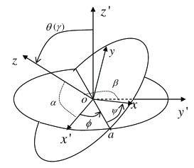
Fig. 2: The ”$x$-convention” of Euler angles. The first rotation is by angle $\phi$ about the $z^{\prime}$-axis, the second rotation is by an angle $\theta\in[0,\pi]$ about the former $x$-axis (now $oa$), and the third rotation is by an angle $\psi$ about the $z$-axis. $\alpha$, $\beta$ and $\gamma$ are the direction angles of $z$-axis in the principle coordinate system $(x^{\prime},y^{\prime},z^{\prime})$.

Generally, available datas of the dielectric tensor are given in the principle coordinate system $(x^{\prime},y^{\prime},z^{\prime})$[16], in which $\hat{\varepsilon}^{\prime}$ is of a diagonal form, but the paraxial equation Eg. (28) for the optical beam is obtained in the propagation coordinate system $(x,y,z)$. To discuss the problem, therefore, the dielectric tensor should be transformed from the principal coordinate system to the propagation coordinate system, in which the dielectric tensor is denoted by $\hat{\varepsilon}$. To do this, we use the so-called ”$x$-convention” definition of the Euler angles $(\phi,\theta,\psi)$ [17], as shown in Fig. 2. In this convention, the coordinate rotation can be written as

$$\left(\begin{array}[]{c}x\\ y\\ z\\ \end{array}\right)=\mathbf{T}\left(\begin{array}[]{c}x^{\prime}\\ y^{\prime}\\ z^{\prime}\\ \end{array}\right),$$ (29)

with the rotation matrix $\mathbf{T}$,

$$\mathbf{T}=\left(\begin{array}[]{ccc}\cos\psi\cos\phi-\cos\theta\sin\phi\sin\psi&\cos\psi\sin\phi+\cos\theta\cos\phi\sin\psi&\sin\psi\sin\theta\\ -\sin\psi\cos\phi-\cos\theta\sin\phi\cos\psi&\cos\theta\cos\phi\cos\psi-\sin\psi\sin\phi&\cos\psi\sin\theta\\ \sin\theta\sin\phi&-\sin\theta\cos\phi&\cos\theta\\ \end{array}\right).$$ (30)

Through the angles $\phi$ and $\theta$, we can rotate the $z^{\prime}$ -coordinate axis to the $z$ -coordinate axis, i.e. the direction of the central wave vector $\mathbf{k}_{0}$. In the principle coordinate system, a given propagation direction $\mathbf{k}_{0}/|\mathbf{k}_{0}|$ is described by the direction cosines $(\cos\alpha,\cos\beta,\cos\gamma)$, then the values of Euler angles $\phi$ and $\theta$ can be obtained from the relation

$$\theta = \gamma$$ (31a)

$$\tan\phi = -\frac{\cos\alpha}{\cos\beta}.$$ (31b)

The nutation angle $\psi$ of the final rotation can be arbitrary chosen since it is used for the orientation of the $x$ and $y$ axes. In general, it is chosen to align the $x$ and $y$ coordinates with the two orthogonal eigenvectors, and these special values of $\psi$, satisfy

$$\tan\psi_{0}=\frac{-(\sigma\cot\phi+\tan\phi)}{(1-\sigma)\cos\theta},$$ (32)

with $\sigma=(n_{1}^{2}-\varepsilon_{x^{\prime}})\varepsilon_{y^{\prime}}[(n_{1}^{2}-\varepsilon_{y^{\prime}})\varepsilon_{x^{\prime}}]^{-1}$. The angle $\psi_{0}$ is to be distinguished from $\psi$ which can be chosen arbitrarily in defining the propagation coordinate system. If $\psi=\psi_{0}$, we have $\mathbf{D}_{1}/|\mathbf{D}_{1}|$ along $x$-axis and $\mathbf{D}_{2}/|\mathbf{D}_{2}|$ along $y$-axis, respectively. As a result, $\psi_{0}$ can be used to denote the directions of the two eigenvectors in propagation coordinate system.

With the coordinates rotation, the dielectric tensor in the propagation coordinate system becomes

$$\hat{\varepsilon}=\mathbf{T}\hat{\varepsilon}^{\prime}\mathbf{T^{-1}}=\left(\begin{array}[]{ccc}\varepsilon_{11}&\varepsilon_{12}&\varepsilon_{13}\\ \varepsilon_{12}&\varepsilon_{22}&\varepsilon_{23}\\ \varepsilon_{13}&\varepsilon_{23}&\varepsilon_{33}\end{array}\right),$$ (33)

where $\mathbf{T^{-1}}$ is the inverse matrix of $\mathbf{T}$, and the components of $\hat{\varepsilon}$ are, respectively,

$$\varepsilon_{11} = (\cos\psi\sin\phi-\cos\theta\sin\psi\sin\phi)^{2}\varepsilon_{x^{\prime}}$$

$$+(\cos\theta\cos\phi\sin\psi+\cos\psi\sin\phi)^{2}\varepsilon_{y^{\prime}}+\sin^{2}\theta\sin^{2}\psi\varepsilon_{z^{\prime}},$$

$$\varepsilon_{12} = (-\cos\phi\sin\psi-\cos\theta\cos\psi\sin\phi)(\cos\psi\cos\phi-\cos\theta\sin\psi\sin\phi)\varepsilon_{x^{\prime}}$$

$$+(\cos\theta\cos\phi\sin\psi+\cos\psi\sin\phi)(\cos\theta\cos\psi\cos\phi-\sin\psi\sin\phi)\varepsilon_{y^{\prime}}$$

$$+\cos\psi\sin^{2}\theta\sin\psi\varepsilon_{z^{\prime}},$$

$$\varepsilon_{13} = (\cos\psi\cos\phi-\cos\theta\sin\psi\sin\phi)\sin\theta\sin\phi\varepsilon_{x^{\prime}}$$

$$-\cos\phi\sin\theta(\cos\theta\cos\phi\sin\psi+\cos\psi\sin\phi)\varepsilon_{y^{\prime}}+\cos\theta\sin\theta\sin\psi\varepsilon_{z^{\prime}},$$

$$\varepsilon_{22} = (-\cos\phi\sin\psi-\cos\theta\cos\psi\sin\phi)^{2}\varepsilon_{x^{\prime}}$$

$$+(\cos\theta\cos\psi\cos\phi-\sin\psi\sin\phi)^{2}\varepsilon_{y^{\prime}}+\cos^{2}\psi\sin^{2}\theta\varepsilon_{z^{\prime}},$$

$$\varepsilon_{23} = (\cos\phi\sin\psi-\cos\theta\cos\psi\sin\phi)\sin\theta\sin\phi\varepsilon_{x^{\prime}}$$

$$-\cos\phi\sin\theta(\cos\theta\cos\psi\cos\phi-\sin\psi\sin\phi)\varepsilon_{y^{\prime}}+\cos\theta\cos\psi\sin\theta\varepsilon_{z^{\prime}},$$

$$\varepsilon_{33} = \sin^{2}\theta\sin^{2}\phi\varepsilon_{x^{\prime}}+\cos^{2}\phi\sin^{2}\theta\varepsilon_{y^{\prime}}+\cos^{2}\theta\varepsilon_{z^{\prime}}.$$

Substituting Eg. (33) into Eg. (4), we get the dispersion relationship in propagation coordinate system. The expressions of $\delta$ coefficients can be obtained from the procedure that introduced in the last paragraph in section 3.A. Since the calculation is complicated, we just present the results here:

$$\delta_{x}=\frac{\varepsilon_{13}\varepsilon_{22}-\varepsilon_{12}\varepsilon_{23}-\varepsilon_{13}n_{j}^{2}}{2\varepsilon_{33}n_{j}^{2}-\varepsilon_{11}\varepsilon_{33}-\varepsilon_{22}\varepsilon_{33}+\varepsilon_{13}^{2}+\varepsilon_{23}^{2}},$$ (34a)

$$\delta_{y}=\frac{\varepsilon_{11}\varepsilon_{23}-\varepsilon_{12}\varepsilon_{13}-\varepsilon_{23}n_{j}^{2}}{2\varepsilon_{33}n_{j}^{2}-\varepsilon_{11}\varepsilon_{33}-\varepsilon_{22}\varepsilon_{33}+\varepsilon_{13}^{2}+\varepsilon_{23}^{2}},$$ (34b)

$$\delta_{xx}=\frac{1}{k_{0}}\left[\frac{-\varepsilon_{12}^{2}-\varepsilon_{13}^{2}+\varepsilon_{11}(\varepsilon_{22}+\varepsilon_{33})-n_{j}^{2}(\varepsilon_{11}+\varepsilon_{33})-4n_{j}^{2}\delta_{x}(\varepsilon_{13}+\varepsilon_{33}\delta_{x})}{2\varepsilon_{33}n_{j}^{2}-\varepsilon_{11}\varepsilon_{33}-\varepsilon_{22}\varepsilon_{33}+\varepsilon_{13}^{2}+\varepsilon_{23}^{2}}+\delta_{x}^{2}\right],$$ (34c)

$$\delta_{yy}=\frac{1}{k_{0}}\left[\frac{-\varepsilon_{12}^{2}-\varepsilon_{23}^{2}+\varepsilon_{22}(\varepsilon_{11}+\varepsilon_{33})-n_{j}^{2}(\varepsilon_{22}+\varepsilon_{33})-4n_{j}^{2}\delta_{y}(\varepsilon_{23}+\varepsilon_{33}\delta_{y})}{2\varepsilon_{33}n_{j}^{2}-\varepsilon_{11}\varepsilon_{33}-\varepsilon_{22}\varepsilon_{33}+\varepsilon_{13}^{2}+\varepsilon_{23}^{2}}+\delta_{y}^{2}\right],$$ (34d)

$$\delta_{xy}=\frac{1}{k_{0}}\left[\frac{\varepsilon_{12}\varepsilon_{33}-\varepsilon_{13}\varepsilon_{23}-n_{j}^{2}\varepsilon_{12}-2n_{j}^{2}\varepsilon_{23}\delta_{x}-2n_{j}^{2}\varepsilon_{13}\delta_{y}-4n_{j}^{2}\varepsilon_{33}\delta_{x}\delta_{y}}{2\varepsilon_{33}n_{j}^{2}-\varepsilon_{11}\varepsilon_{33}-\varepsilon_{22}\varepsilon_{33}+\varepsilon_{13}^{2}+\varepsilon_{23}^{2}}+\delta_{x}\delta_{y}\right],$$ (34e)

where $k_{0}=n_{j}\omega/c$ with $n_{j}$ given by Eg. (15). If $n_{1}$ is substituted, we will obtain a set of $\delta$ coefficients for the mode 1 beam and that for the mode 2 beam with $n_{2}$ substituted. In particular, $\psi=\psi_{0}$ can reduce the $\delta$ coefficients to the same forms that presented in [9].

Eg. (28) together with the $\delta$ coefficients describes the paraxial beam propagating in a general direction except along the optics axes in a general anisotropic medium. In the uniaxial case, for example, the positive uniaxial crystal with $\varepsilon_{x^{\prime}}=\varepsilon_{y^{\prime}}=n_{o}^{2}$ and $\varepsilon_{z^{\prime}}=n_{e}^{2}$ in $\hat{\varepsilon}^{\prime}$, the mode 1 beam turns out to be the ordinary beam with $n_{1}$ reduced to $n_{o}$, and the $\delta$ coefficients are reduced to $\delta_{xx}=\delta_{yy}=-c/(\omega n_{o})$ and zero of the others, then we obtain the standard paraxial equation for the ordinary beam,

$$i\frac{\partial A}{\partial z}+\frac{c}{2\omega n_{o}}\left(\frac{\partial^{2}A}{\partial x^{2}}+\frac{\partial^{2}A}{\partial y^{2}}\right)A=0.$$ (35)

On the other hand, the mode 2 beam is the extraordinary beam with the $\delta$ coefficients reduced to

$$\delta_{x}=\frac{(n_{o}^{2}-n_{e}^{2})\sin\psi\sin 2\theta}{2(n_{o}^{2}\sin^{2}\theta+n_{e}^{2}\cos^{2}\theta)},$$ (36a)

$$\delta_{y}=\frac{(n_{o}^{2}-n_{e}^{2})\cos\psi\sin 2\theta}{2(n_{o}^{2}\sin^{2}\theta+n_{e}^{2}\cos^{2}\theta)},$$ (36b)

$$\delta_{xx}=-\frac{1}{k^{(e)}_{0}}\frac{n_{o}^{4}\cos^{2}\psi\sin^{2}\theta+n_{o}^{2}n_{e}^{2}(\sin^{2}\psi\sin^{2}\theta+\cos^{2}\theta)}{(n_{o}^{2}\sin^{2}\theta+n_{e}^{2}\cos^{2}\theta)^{2}},$$ (36c)

$$\delta_{yy}=-\frac{1}{k^{(e)}_{0}}\frac{n_{o}^{4}\sin^{2}\psi\sin^{2}\theta+n_{o}^{2}n_{e}^{2}(\cos^{2}\psi\sin^{2}\theta+\cos^{2}\theta)}{(n_{o}^{2}\sin^{2}\theta+n_{e}^{2}\cos^{2}\theta)^{2}},$$ (36d)

$$\delta_{xy}=\frac{1}{k^{(e)}_{0}}\frac{n_{o}^{2}(n_{o}^{2}-n_{e}^{2})\sin 2\psi\sin^{2}\theta}{2(n_{o}^{2}\sin^{2}\theta+n_{e}^{2}\cos^{2}\theta)^{2}},$$ (36e)

where $k^{(e)}_{0}=n^{(e)}\omega/c$ and

$$n^{(e)}=\frac{n_{o}n_{e}}{(n_{o}^{2}\sin^{2}\theta+n_{e}^{2}\cos^{2}\theta)^{1/2}}$$ (37)

is the refractive index with the form expressed in the propagation coordinate system. Eg. (37) is obtained by making the coordinate transformation on $n_{2}$ after it has been reduced under the uniaxial condition. Here we pay some attention on the results for the extraordinary beam. The symmetry about the $z^{\prime}$-axis of the index ellipsoid makes the propagation direction only described by $\theta$, so the $\delta$ coefficients are independent on the angle $\phi$. For the coefficient $\delta_{xy}$, Eg. (36e) shows that once $\theta$ is specified, its value is modified by the angle $\psi$ and the sine function makes the value periodic. To physically understand these properties, we recall that the wave vectors of the extraordinary plane waves belong to an extraordinary ellipsoid of semi axes $n_{o}\omega/c$, $n_{e}\omega/c$ and $n_{e}\omega/c$, of which the surface is called the normal surface [15]. For the extraordinary beam, the curved surface of the ellipsoid near the central wave vector $\mathbf{k}^{(e)}_{0}$ is not rotational symmetry about $\mathbf{k}^{(e)}_{0}$ if $\mathbf{k}^{(e)}_{0}$ is not along the optical axis. Therefore, the mixed derivatives terms arise in the Taylor expansion Eg. (23) for a general $\psi$, and its periodic characteristic is readily understood by recalling that the orientation of the $x$ and $y$ axes repeat again if $\psi$ increase from zero to $2\pi$. The coefficient $\delta_{xy}$ in the case of biaxial media has the similar properties but it is not evident from Eg. (34e).

In this uniaxial case, Eg. (19) implies that the optical axis coincides with the $z^{\prime}$-axis. If we set $\psi=\pi/2$ which lies the $x$-axis in the plane that formed by the optic axis and the $z$-axis, and substitute (38) into Eg. (28), we will get the wave equation for the extraordinary beam which is equal to the linear part of the nonlinear equation obtained by Qi Guo and Sien Chi (Eq. (42) in [10]),

$$i\bigg{[}\frac{\partial A}{\partial z}-\frac{(n_{o}^{2}-n_{e}^{2})\sin 2\theta}{2(n_{o}^{2}\sin^{2}\theta+n_{e}^{2}\cos^{2}\theta)}\frac{\partial A}{\partial x}\bigg{]}-\frac{cn_{o}^{2}}{2\omega n^{(e)}}\bigg{[}\frac{n_{e}^{2}}{(n_{o}^{2}\sin^{2}\theta+n_{e}^{2}\cos^{2}\theta)^{2}}\frac{\partial^{2}A}{\partial x^{2}}$$

$$+\frac{1}{n_{o}^{2}\sin^{2}\theta+n_{e}^{2}\cos^{2}\theta}\frac{\partial^{2}A}{\partial y^{2}}\bigg{]}=0.$$ (38)

Further more, $\theta=\pi/2$ will reduce Eg. (3.B) to the form of describing the paraxial beam propagation orthogonal to the optical axis, which is the same result given by the equation (8) in reference [6].

4 Elliptical Gaussian beam propagation

The properties of paraxial beam propagation in anisotropic media will be fully elucidated by using a specified input field. In the first subsection, we will use an initial elliptic Gaussian field for investigation and obtain the analytic solution. We find that the elliptic Gaussian beam will rotate during propagation and the rotation is discussed in detail. In the second subsection, we will give some examples for illustration.

4.A Analytic solution of initial elliptic Gaussian beam

We discuss the elliptic Gaussian beam propagation in anisotropic media. Suppose that the input field at $z=0$ is given by

$$\mathbf{E}_{0}(x,y,0)=\mathbf{p}_{0}A_{0}\exp\left(\frac{-x^{2}}{2w_{x}^{2}}\right)\exp\left(\frac{-y^{2}}{2w_{y}^{2}}\right),$$ (39)

where $w_{x}$ and $w_{y}$ are the initial beam widths in $x$ and $y$ directions, respectively, and for convenience, $w_{x}>w_{y}$; $A_{0}$ is the amplitude of the field. With this input field, the analytic solution of Eg. (28) is [7]

$${A}(x,y,z)=A_{0}\frac{\exp\left\{\frac{-[X+i\delta_{xy}Yz/(w_{y}^{2}-i\delta_{yy}z)]^{2}}{2[w_{x}^{2}-i\delta_{xx}z+\delta_{xy}^{2}z^{2}/(w_{y}^{2}-i\delta_{yy}z)]}\right\}\exp\left[\frac{-Y^{2}}{2(w_{y}^{2}-i\delta_{yy}z)}\right]}{\sqrt{[w_{x}^{2}-i\delta_{xx}z+\delta_{xy}^{2}z^{2}/(w_{y}^{2}-i\delta_{yy}z)](w_{y}^{2}-i\delta_{yy}z)}},$$ (40)

where $X=x+\delta_{x}z$, $Y=y+\delta_{y}z$, respectively. To investigate the field evolution, we should first obtain the modulus of the complex expression Eg. (40), which reads

$$|{A}(x,y,z)|=\frac{\exp\left[-\left(\frac{B_{1}}{2B}X^{2}+\frac{B_{2}}{2B}Y^{2}+\frac{B_{3}}{B}XY\right)\right]}{\sqrt{B}},$$ (41)

where

$$B_{1} = w_{x}^{2}w_{y}^{4}+z^{2}w_{x}^{2}\delta_{yy}^{2}+z^{2}w_{y}^{2}\delta_{xy}^{2},$$

$$B_{2} = w_{x}^{4}w_{y}^{2}+z^{2}w_{y}^{2}\delta_{xx}^{2}+z^{2}w_{x}^{2}\delta_{xy}^{2},$$

$$B_{3} = -z^{2}\delta_{xy}(w_{y}^{2}\delta_{xx}+w_{x}^{2}\delta_{yy}),$$

$$B = z^{2}(w_{x}^{2}\delta_{yy}+w_{y}^{2}\delta_{xx})^{2}+[w_{x}^{2}w_{y}^{2}+z^{2}(\delta_{xy}^{2}-\delta_{xx}\delta_{yy})]^{2}.$$

The quadratic form of the exponent shows that the field distribution is a rotated ellipse in $X-Y$ plane if $B_{3}\neq 0$. $B_{3}$ is proportional to $\delta_{xy}$, so $\delta_{xy}=0$ for no rotation. The rotation angle $\varphi$, defined as the tilt of the major axis relative to $X$-axis, satisfies

$$\tan 2\varphi = \frac{B_{3}}{B_{1}-B_{2}}$$ (42)

$$= \frac{2z^{2}\delta_{xy}(w_{y}^{2}\delta_{xx}+w_{x}^{2}\delta_{yy})}{w_{x}^{4}w_{y}^{2}-w_{x}^{2}w_{y}^{4}+z^{2}w_{y}^{2}(\delta_{xx}^{2}-\delta_{xy}^{2})-z^{2}w_{x}^{2}(\delta_{yy}^{2}-\delta_{xy}^{2})}.$$

A word of conventions is needed here. The rotation angle $\varphi$ determined by Eg. (42) has a range within $\pm\pi/2$, so it will be the convention of this paper to fix the quantity unambiguously by defining the arctangent function as having a range lying in the interval $[-\pi,+\pi]$. On this convention, the major to semimajor axes ratio $\eta$ of the rotated ellipse is

$$\eta=\left(\frac{B_{1}\sin^{2}\varphi+B_{2}\cos^{2}\varphi-\frac{1}{2}B_{3}\sin 2\varphi}{B_{1}\cos^{2}\varphi+B_{2}\sin^{2}\varphi+\frac{1}{2}B_{3}\sin 2\varphi}\right)^{1/2}.$$ (43)

When $\delta_{xy}\neq 0$, the rotation velocity, described by $\partial\varphi/\partial z$, can be obtained from the derivative of Eg. (42) with respect to $z$,

$$\frac{\partial\varphi}{\partial z}=\frac{2\cos^{2}(2\varphi)zw_{x}^{2}w_{y}^{2}(w_{x}^{2}-w_{y}^{2})\delta_{xy}(w_{y}^{2}\delta_{xx}+w_{x}^{2}\delta_{yy})}{\left[w_{x}^{4}w_{y}^{2}-w_{x}^{2}w_{y}^{4}+z^{2}w_{y}^{2}(\delta_{xx}^{2}-\delta_{xy}^{2})-z^{2}w_{x}^{2}(\delta_{yy}^{2}-\delta_{xy}^{2})\right]^{2}}.$$ (44)

Generally, the diffraction coefficients $\delta_{xx}$ and $\delta_{yy}$ are negatives, making the beam spread in the medium. As a result, the rotation direction is determined by the coefficient $\delta_{xy}$ which is directly associated with the angle $\psi$ while the propagation direction has been specified. For a chosen $\psi$, if $\delta_{xy}<0$, we have $\partial\varphi/\partial z>0$, implying that the beam will rotate counterclockwise. On the contrary, $\delta_{xy}>0$ is corresponding to the clockwise rotation of the beam. For large $z$, Eg. (42) is approximate to

$$\tan 2\varphi\approx\frac{2\delta_{xy}(\delta_{xx}+\frac{w_{x}^{2}}{w_{y}^{2}}\delta_{yy})}{\delta_{xx}^{2}-\frac{w_{x}^{2}}{w_{y}^{2}}\delta_{yy}^{2}+(\frac{w_{x}^{2}}{w_{y}^{2}}-1)\delta_{xy}^{2}}.$$ (45)

Eg. (45) shows that the rotation angle will approach a value that depends on the ratio of the initial beam widths $w_{x}/w_{y}$. As a special case, when the input field is a circular Gaussian beam, i.e. $w_{x}=w_{y}$, it can be proved directly from Eg. (40) that the input field will lose its circular symmetry during propagation and become elliptical. This is because the physical properties of the diffractive spreading (described by $\delta_{xx}$, $\delta_{yy}$, $\delta_{xy}$) are different in every transverse directions in an anisotropic media. With $w_{x}=w_{y}$, Eg. (42) gives

$$\tan 2\varphi=\frac{2\delta_{xy}}{\delta_{xx}-\delta_{yy}}.$$ (46)

The rotation angle is independent on $z$, so the beam will not rotate but incline by an unvaried angle during propagation.

For the case of $\delta_{xy}=0$, Eg. (40) can be factorized into the product of two one-dimensional Gaussian beams. In such case, the beam will not rotate but just spread in $x$ and $y$ directions with the diffraction coefficients $\delta_{xx}$ and $\delta_{yy}$, respectively.

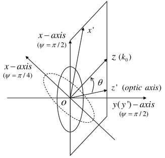
Fig. 3: Different values of $\psi$ correspond to different input fields for the extraordinary beam in uniaxial crystal. For $\psi=\pi/4$, the input field Eg. (39) corresponds to the dashed ellipse and this beam will rotate during propagation; for $\psi=\pi/2$, the input field Eg. (39) corresponds to the solid ellipse and this beam will not rotate during propagation

Here we should remind that the angle $\psi$ can be freely chosen and plays a role of fixing the $x$ and $y$ axes. Since the input field Eg. (39) is of a regular form in the propagation coordinate system, different values of $\psi$ correspond to different input fields. If we choose a value of $\psi$ that makes $\delta_{xy}\neq 0$, then the input elliptic Gaussian beam will rotate during propagation, otherwise, there will be no rotation effect on the beam. To illuminate the relationship between $\psi$ and the input field, we still take the extraordinary beam in the positive uniaxial crystal for example. The $\delta$ coefficients for the beam are given by Eq. (36). We can obtain from Eg. (36e) that $\delta_{xy}=0$ if $\psi=m\pi/2$, where $m=0,1,2,3$. If $\psi$ takes one of these values, which corresponds to lying one of the waists ($w_{x}$ or $w_{y}$) in the plane that formed by the optic axis and $\mathbf{k}_{0}$, see Fig. 3, the extraordinary beam will propagate with no rotation effect (as the case of $\psi=\pi/2$). Otherwise, the extraordinary beam will rotate during propagation (as the case of $\psi=\pi/4$). The cases of the biaxial media are similar except that the values of $\psi$ for $\delta_{xy}=0$ are different from that in the uniaxial cases.

4.B Examples

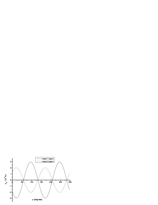
Fig. 4: $\delta_{xy}$ as a function of $\psi$ with $\phi=109.50^{\circ}$ and $\theta=6.00^{\circ}$

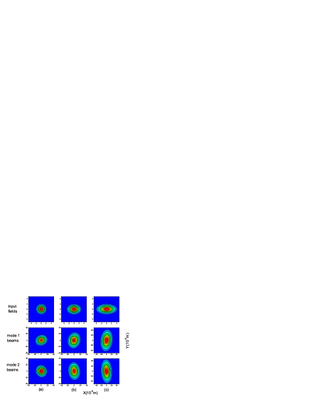
Fig. 5: (Color online)Elliptical beams propagation with different spatial widths of the input fields: (a)$w_{x}:w_{y}=1:1$, (b) $w_{x}:w_{y}=1.4:1$, (c) $w_{x}:w_{y}=2:1$, where $w_{y}=10.0\mu\rm{m}$. The contour plots of $|\mathbf{A}(x,y,z)|$ are taken at $\xi=10$. The $\delta$ coefficients are, for the mode 1 beam: $\delta_{x}=1.549\times 10^{-2}$, $\delta_{y}=6.557\times 10^{-3}$, $\delta_{xx}=-3.906\times 10^{-8}\rm{m}$, $\delta_{yy}=-3.486\times 10^{-8}\rm{m}$, $\delta_{xy}=-2.095\times 10^{-9}\rm{m}$; for the mode 2 beam: $\delta_{x}=-1.585\times 10^{-3}$, $\delta_{y}=3.745\times 10^{-3}$, $\delta_{xx}=-3.565\times 10^{-8}\rm{m}$, $\delta_{yy}=-3.855\times 10^{-8}\rm{m}$, $\delta_{xy}=1.427\times 10^{-9}\rm{m}$, respectively.

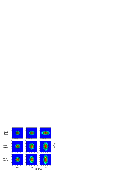
Fig. 6: (Color online)Similar to figure 5 except with $\psi=69.48^{\circ}$. The $\delta$ coefficients are, for the mode 1 beam: $\delta_{x}=1.682\times 10^{-2}$, $\delta_{y}=1.349\times 10^{-4}$, $\delta_{xx}=-3.992\times 10^{-8}\rm{m}$, $\delta_{yy}=-3.400\times 10^{-8}\rm{m}$; for the mode 2 beam: $\delta_{x}=-4.639\times 10^{-5}$, $\delta_{y}=4.067\times 10^{-3}$, $\delta_{xx}=-3.507\times 10^{-8}\rm{m}$, $\delta_{yy}=-3.913\times 10^{-8}\rm{m}$, respectively.

Here we will use some examples to illustrate the properties of the propagation that discussed above. For more general, we show the beams propagation in the biaxial crystal $\rm{KNbO}_{3}$. The wavelength of the input beams is $\lambda=514\rm{nm}$, and for this wavelength, the elements of the dielectric tensor in principle coordinate system are reported as $\varepsilon_{x^{\prime}}=5.736$, $\varepsilon_{y^{\prime}}=5.446$, $\varepsilon_{z^{\prime}}=4.893$ [16] which place the optic axes at $\alpha_{c}=\pm 56.21^{\circ}$. The optical beam is supposed to propagate along a general direction $(\alpha,\beta,\gamma)=(84.36^{\circ},88^{\circ},6^{\circ})$ in the principle coordinate system. This direction is arbitrary chosen but should not be too close to the optic axes. It will be convenient to use this direction in all examples. The refractive indices of the two eigenmodes are $n_{1}=2.393$ and $n_{2}=2.334$. According to Eg. (31), the first two Euler angles are $\phi=109.50^{\circ}$, $\theta=6.00^{\circ}$, and from Eg. (32), we have $\psi_{0}=69.94^{\circ}$ . Fig. 4 shows the parameter $\delta_{xy}$ versus the angle $\psi$ in the supposed propagation direction. As shown, there are four roots for $\delta_{xy}=0$ which are $69.48^{\circ}+m90^{\circ}$, with $m=0,1,2,3$. To accentuate the physics of the $\delta_{xy}$ term, we take $\psi=47^{\circ}$ in the first example to show the propagation of beam with $\delta_{xy}\neq 0$, and then $\psi=69.48^{\circ}$ is taken in the second example for comparison. The $\delta$ coefficients are evaluated by (34a)- (34e), and the propagation is computed by using Eg. (40) with the propagation distance normalized by $\xi=zc[\omega(w_{x}^{2}+w_{y}^{2})]^{-1}$. The results are shown in Fig. 5 and Fig. 6 in which the coordinate frames move with the centers of the beams, so the walk-off of the beams are not shown in the figures.

Fig. 5 shows the propagation of the two beams of different modes with three different initial beam widths. Fig. 5(a) is the case of the initial circular Gaussian fields. We can see that after the propagation, the initially circular cross-sections of the two modes both become elliptical and inclined. The unvaried inclined angles given by Eg. (46) are the same, both are equal to $22.48^{\circ}$. Figures 5(b) and (c) show the propagation of the initial elliptical Gaussian beams. The mode 1 beams rotate counterclockwise and the mode 2 beams rotate clockwise, as predicted by Eg. (44). For $\xi=10$, the propagation distant is long enough that the rotation angles can be approximately obtained by Eg. (45): the rotation angles for the mode 1 beams are $\varphi\approx 76.09^{\circ}$ in (b) and $\varphi\approx-83.65^{\circ}$ in (c), and for the mode 2 beams, they are $\varphi\approx-84.52^{\circ}$ in (b) and $\varphi\approx-86.69^{\circ}$ in (c), respectively. Fig. 6 shows the cases of $\delta_{xy}=0$. As expected, there is no rotation or inclination effect on the beams. The beams just spread in the $X$ and $Y$ directions.

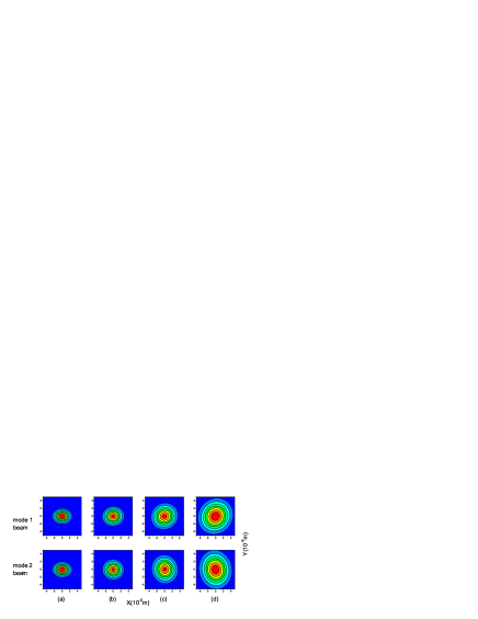
Fig. 7: (Color online) Contour of magnitude of the slowly varying amplitude $|\mathbf{A}(\mathbf{r})|$, for an initial Gaussian beam with $\lambda=514\rm{nm}$,$\psi=109.50^{\circ}$, $\theta=6.00^{\circ}$, and $\psi=47.00^{\circ}$. Spatial widths $w_{x}=12.5\mu\rm{m}$ and $w_{y}=10\mu\rm{m}$ in the frame moving with the center of the beam for (a)$\xi=0$, (b)$\xi=0.734$, (c)$\xi=1.277$, (d)$\xi=1.915$.

To get a full picture of the beam rotation, we present the details in the following examples. The parameters are the same as those in Fig. 5 except with $w_{x}=12.5\mu\rm{m}$ and $w_{y}=10.0\mu\rm{m}$. The results are shown in Fig. 7 which contains four plots with different $\xi$ for each mode. The mode 1 beam rotates counterclockwise. The rotation angle increases with increasing $\xi$ and the cross-section keeps elliptical during propagation. The mode 2 beam has a clockwise rotation. For $\xi=0.734$, the mode 2 beam has broadened in $Y$ due to Fresnel diffraction $\delta_{yy}$ and is roughly as broad in $X$ as in $Y$. Therefore, the tilt of the beam is difficult to see in Fig. 7(b). As the propagation proceeds, the rotation becomes evident again, as shown in Fig. 7(c) and (d).

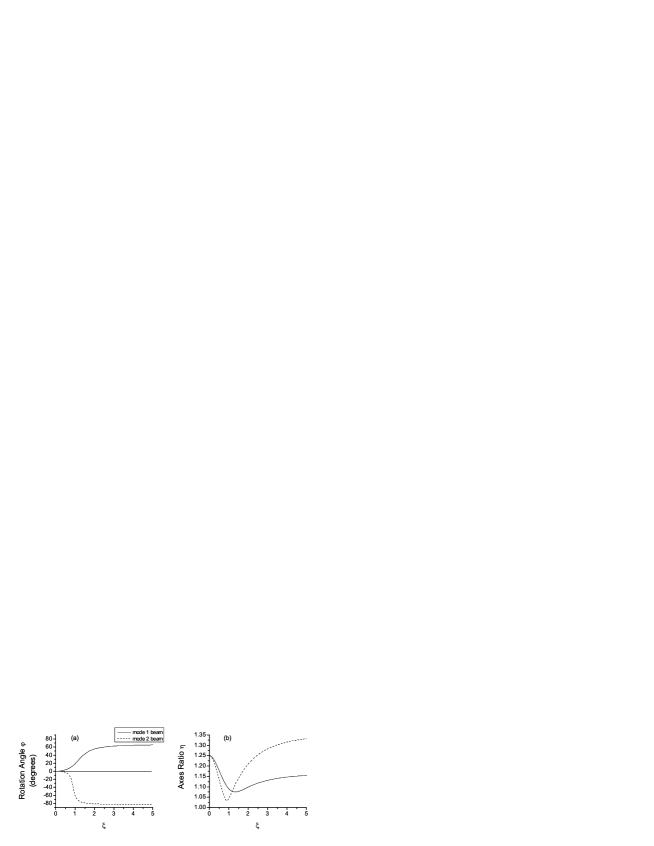
Fig. 8: (a)Rotation angle $\varphi$ as a function of $\xi$. (b) major to semi major axes ratio $\eta$. Solid curve for the mode 1 beam and dashed curve for the mode 2 beam.

Fig. 8(a) shows the rotation angles versus $\xi$. It indicates that the rotation angles increase (the mode 1 beam) or decrease (the mode 2 beam) monotonously with the increasing $\xi$, and for large $\xi$, they both approach certain values which are given by Eg. (46), respectively. For the mode 1 beam, $\varphi\approx 66.73^{\circ}$, and $\varphi\approx-82.69^{\circ}$ for the mode 2 beam. Fig. 8(b) shows the major to semimajor axes ratio $\eta$ of the ellipse describing the contour lines of $|\mathbf{A}(x,y,z)|$. Both of the ratios share the same characteristics that each of them initially decreases due to the diffraction and goes through a minimum. Fig. 8(a) together with (b) shows that before the $\delta_{xy}$ term makes an obvious rotation on the cross-section of the beam (for example, $\varphi\approx 45^{\circ}$), $\eta$ has dramatically decreased and approached the minimum value, i.e. the ellipticity decreases. This is because the diffraction will exercise the most influence on the evolution of the beam rather than the rotation effect if the coefficient $\delta_{xy}$ is much smaller than $\delta_{xx}$ (or $\delta_{yy}$). Although the rotation will become evident with $\xi$ increasing, the initial rotation effect is strongly influenced by diffraction and is barely visible (like the mode 2 beam in Fig. 7(a) and (b)). As a result, in our examples we choose the spacial widths of the initial field ($w_{x}$ and $w_{y}$) to be close to each other so that the diffraction effect is not so strong to influence the observation of the rotation. The process of beam rotation shown in Fig. 7 may be not so obvious, but we think the examples are sufficient to elucidate the physics.

An obvious beam rotation can be observed if coefficient $\delta_{xy}$ is comparable to $\delta_{xx}$ or $\delta_{yy}$ in magnitude. In order to find a large $\delta_{xy}$, we examine the ratio $\delta_{xy}/\delta_{xx}$ ($\delta_{yy}$ is on the order of $\delta_{xx}$). The ratio is a function of the the Euler angles with the maximum determined by $(\varepsilon_{x}-\varepsilon_{z})/[2(\varepsilon_{x}\varepsilon_{z})^{1/2}]$ which is associated with the degree of anisotropy. According to this value, we find that in many natural biaxial crystals like $\rm{KTP}$, $\rm{LBO}$ or $\rm{LiNbO}_{3}$ [16], $\delta_{xy}$ is at least one order less than $\delta_{xx}$. To our knowledge, natural material with large $\delta_{xy}$ is not readily available yet. However, in recent scientific progress, metamaterial technology revolutionized modern optics and photonics by creating nearly unlimited opportunities for engineering material parameters. The electric and magnetic properties can be carefully designed and tuned by changing the geometry, size and other characteristics of meta-atoms [18, 19]. As a result, material with large coefficient $\delta_{xy}$ might be realized. For example, supposed that a kind of metamaterial with a dielectric tenser

$$\hat{\varepsilon}^{\prime}=\left[\begin{array}[]{ccc}6&0&0\\ 0&4&0\\ 0&0&2\\ \end{array}\right]$$

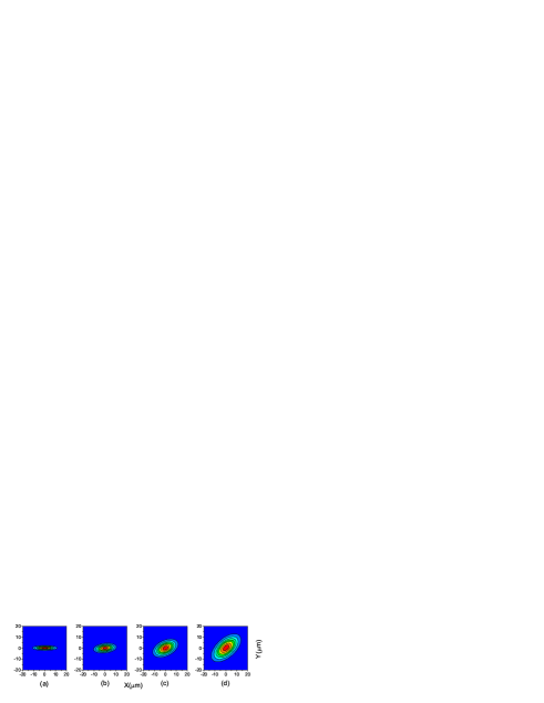
Fig. 9: (Color online) Propagation of mode 1 beam in the assumed metamaterial. Spatial widths are $w_{x}=5\mu\rm{m}$ and $w_{y}=1\mu\rm{m}$ in the frame moving with the center of the beam for (a)$\xi=0$, (b)$\xi=0.160$, (c)$\xi=0.315$, (d)$\xi=0.478$.

has been engineered, according to our theory above, in the supposed propagation direction, we have $\delta_{xx}=-8.767\times 10^{-8}$, $\delta_{yy}=-4.107\times 10^{-8}$ and $\delta_{xy}=-2.339\times 10^{-8}$ for the mode 1 beam ($\psi$ is chosen to be equal to$47^{\circ}$). Since $\delta_{xy}$ is comparable to $\delta_{xx}(\delta_{yy})$, we can expect a significant effect from $\delta_{xy}$. We present the propagation of the mode 1 beam in such material in Fig. 9. As expected, the inclination is obvious.

Through these examples, we can see that the coefficient $\delta_{xy}$ will play an rotation effect on the beam propagation if it is nonvanishing. Although here we just present the propagation of elliptical Gaussian beam, many other simulations can be made with the beam equation in biaxial media or uniaxial media, for example, the propagation of higher-order modes of Hermit-Gaussian beams, we don’t present the results here.

5 Conclusion

We investigate the propagation of paraxial beam in anisotropic media. The propagation equation contains terms that account for the beam walk-off, Fresnel diffraction and beam rotation which is mainly discussed in this paper. The term responsible for the rotation originates from the finite beam size and the refractive index depending on the propagation direction. As a result, this term vanishes for the wave in isotropic media and for the ordinary wave in uniaxial media; it is nonvanishing for the extraordinary wave in uniaxial media and the waves in biaxial media. We investigate this rotation effect by using an initial elliptical Gaussian beam in the biaxial media $\rm{KNbO}_{3}$. The analytical solution shows that the initial elliptical cross-section of the beam keeps elliptical and rotates clockwise or counterclockwise during propagation, and for large propagation distance, the rotation angle will asymptotically approach a certain value which depends on the ratio of the initial beam widths. It also shows that an initial circular Gaussian beam will lose its circular symmetry and become elliptical and inclined. This is because the anisotropy makes the properties of diffractive spreading different in every transverse directions. Finally, we point out that the intensity of the rotation is associated with the degree of anisotropy. The rotation will be remarkable with high degree of anisotropy of the media, otherwise, it will be week and may be covered by diffraction.

List of Figure Captions

Fig. 1. (a)Index ellipsoid and (b) the ellipse that the plane $\Sigma$ cuts in the index ellipsoid.

Fig. 2. The ”$x$-convention” of Euler angles. The first rotation is by angle $\phi$ about the $z^{\prime}$-axis, the second rotation is by an angle $\theta\in[0,\pi]$ about the former $x$-axis (now $oa$), and the third rotation is by an angle $\psi$ about the $z$-axis. $\alpha$, $\beta$ and $\gamma$ are the direction angles of $z$-axis in the principle coordinate system $(x^{\prime},y^{\prime},z^{\prime})$.

Fig. 3. Different values of $\psi$ correspond to different input fields for the extraordinary beam in uniaxial crystal. For $\psi=\pi/4$, the input field Eg. (39) corresponds to the dashed ellipse and this beam will rotate during propagation; for $\psi=\pi/2$, the input field Eg. (39) corresponds to the solid ellipse and this beam will not rotate during propagation.

Fig. 4. $\delta_{xy}$ as a function of $\psi$ with $\phi=109.50^{\circ}$ and $\theta=6.00^{\circ}$

Fig. 5. (Color online)Elliptical beams propagation with different spatial widths of the input fields: (a)$w_{x}:w_{y}=1:1$, (b) $w_{x}:w_{y}=1.4:1$, (c) $w_{x}:w_{y}=2:1$, where $w_{y}=10.0\mu\rm{m}$. The contour plots of $|\mathbf{A}(x,y,z)|$ are taken at $\xi=10$. The $\delta$ coefficients are, for the mode 1 beam: $\delta_{x}=1.549\times 10^{-2}$, $\delta_{y}=6.557\times 10^{-3}$, $\delta_{xx}=-3.906\times 10^{-8}\rm{m}$, $\delta_{yy}=-3.486\times 10^{-8}\rm{m}$, $\delta_{xy}=-2.095\times 10^{-9}\rm{m}$; for the mode 2 beam: $\delta_{x}=-1.585\times 10^{-3}$, $\delta_{y}=3.745\times 10^{-3}$, $\delta_{xx}=-3.565\times 10^{-8}\rm{m}$, $\delta_{yy}=-3.855\times 10^{-8}\rm{m}$, $\delta_{xy}=1.427\times 10^{-9}\rm{m}$, respectively.

Fig. 6. (Color online)Similar to figure 5 except with $\psi=69.48^{\circ}$. The $\delta$ coefficients are, for the mode 1 beam: $\delta_{x}=1.682\times 10^{-2}$, $\delta_{y}=1.349\times 10^{-4}$, $\delta_{xx}=-3.992\times 10^{-8}\rm{m}$, $\delta_{yy}=-3.400\times 10^{-8}\rm{m}$; for the mode 2 beam: $\delta_{x}=-4.639\times 10^{-5}$, $\delta_{y}=4.067\times 10^{-3}$, $\delta_{xx}=-3.507\times 10^{-8}\rm{m}$, $\delta_{yy}=-3.913\times 10^{-8}\rm{m}$, respectively.

Fig. 7. (Color online) Contour of magnitude of the slowly varying amplitude $|\mathbf{A}(\mathbf{r})|$, for an initial Gaussian beam with $\lambda=514\rm{nm}$,$\psi=109.50^{\circ}$, $\theta=6.00^{\circ}$, and $\psi=47.00^{\circ}$. Spatial widths $w_{x}=12.5\mu\rm{m}$ and $w_{y}=10\mu\rm{m}$ in the frame moving with the center of the beam for (a)$\xi=0$, (b)$\xi=0.734$, (c)$\xi=1.277$, (d)$\xi=1.915$.

Fig. 8. (a)Rotation angle $\varphi$ as a function of $\xi$. (b) major to semi major axes ratio $\eta$. Solid curve for the mode 1 beam and dashed curve for the mode 2 beam.

Fig. 9. (Color online) Propagation of mode 1 beam in the assumed metamaterial. Spatial widths are $w_{x}=5\mu\rm{m}$ and $w_{y}=1\mu\rm{m}$ in the frame moving with the center of the beam for (a)$\xi=0$, (b)$\xi=0.160$, (c)$\xi=0.315$, (d)$\xi=0.478$.

.

.

References

- [1] J. A. Fleck, Jr. and M. D. Feit ”Beam propagation in uniaxial anisotropic media,” J. Opt. Soc. Am. 73, 920-926 (1983).
- [2] A. Ciattoni, B. Crosignani, and P. D. Porto, ”Vectorial theory of propagation in uniaxially anisotropic media,” J. Opt. Soc. Am. A . 18, 1656-1661 (2001).
- [3] A. Ciattoni, G. Cincotti, C. Palma, and H. Weber, ”Energy exchange between the Cartesian components of a paraxial beam in a uniaxial crystal,” J. Opt. Soc. Am. A . 19, 1894-1900 (2002).
- [4] A. Ciattoni, G. Cincotti, D. Provenziani, and C. Palma, ”Paraxial propagation along the optical axis of a uniaxial medium,” Phys. Rev. E . 66, 036614 (2002).
- [5] G. Cincotti, A. Ciattoni and C. Palma, ”Hermite-Gauss beams in uniaxially anisotropic crystals,” IEEE J. Quantum Electron. 37, 1517-1524 (2001).
- [6] A. Ciattoni, and C. Palma, ”Optical propagation in uniaxial crystals orthogonal to the optical axis: paraxial theory and beyond,” J. Opt. Soc. Am. A . 20, 2163-2171 (2003)
- [7] Y. B. Band and M. Trippenbach, ”Optical Wave-Packet Propagation in Nonisotropic Media,” Phys. Rev. Lett. 76, 1457-1460 (1996)
- [8] M. Trippenbach and Y. B.Band, ”Propagation of light pulses in nonisotropic media,” J. Opt. Soc. Am. B . 13, 1403-1411 (1996).
- [9] M. A. Dreger, ”Optical beam propagation in biaxial crystals,” J. Opt. A: Pure Appl. Opt . 1, 601-616 (1999).
- [10] Q. Guo and S. Chi, ”Nonlinear light beam propagation in unixial crystals: nonlinear refractive index, self-trapping and self-focusing,” J. Opt. A: Pure Appl. Opt. 2, 5-15 (2000).
- [11] I. Tinkelman and T. Melemed ”Gaussian-beam propagation in genetic anisotropic wabe-number profiles,” Opt. Lett. 28, 1081-1083 (2003).
- [12] S. R. Seshadri, ”Basic ellitical Gaussian wave and beam in a uniaxial crystal,” J. Opt. Soc. Am. A . 20, 1818-1826 (2003).
- [13] M. Born and E. Wolf Principle of optics,7th ed (Syndicate of the Press of University of Cambridge, UK. 1999), pp. 790-805.
- [14] A. Yariv and P. Yeh Optical Waves in Crystals, (John Wiley, New York, 1984) ch 4, table 7.1, p 224
- [15] H. A. Haus, Waves and fields in optoelectronics, (Prentice-Hall, Englewood Cliffs, New Jersey, USA, 1984), pp. 298-322.
- [16] W. J. Tropf, M. E. Thomas, and T. J. Harris. ”Properties of crystals and glasses,” in Handbook of Optics , Volume 2, 2nd ed,, M. Bass, E. W. V. Stryland, D. R. Williams and W. L. Wolfe. (McGraw-Hill, USA., 1995). pp. 33.64.
- [17] Weisstein, W. Eric, ”Euler Angles.” From MathWorld–A Wolfram Web Resource. http://mathworld.wolfram.com/EulerAngles.html
- [18] D. H. Werner, D. H. Kwon, I. C. Khoo, A. V. Kildishev and Shalaev, ”Liquid crystal clad near-infrared metamaterials with tunable negative-zero-positive refractive indices,” Opt. Express 15 3342 (2007)
- [19] N. M. Litchinitser and V. M. Shalaev, ”Photonic metamaterials,” Laser Phys. Lett 5 411-20 (2008)