Relativistic redshift effects
and the Galactic-center stars

Abstract

The high pericenter velocities (up to a few percent of light) of the S stars around the Galactic-center black hole suggest that general relativistic effects may be detectable through the time variation of the redshift during pericenter passage. Previous work has computed post-Newtonian perturbations to the stellar orbits. We study the additional redshift effects due to perturbations of the light path (what one may call “post-Minkowskian” effects), a calculation that can be elegantly formulated as a boundary-value problem. The post-Newtonian and post-Minkowskian redshift effects are comparable: both are $\mathcal{O}(\beta^{3})$ and amount to a few $\rm\,km\;s^{-1}$ at pericenter for the star S2. On the other hand, the post-Minkowskian redshift contribution of spin is $\mathcal{O}(\beta^{5})$ and much smaller than the $\mathcal{O}(\beta^{4})$ post-Newtonian effect, which would be $\sim 0.1\rm\,km\;s^{-1}$ for S2.

1 Introduction

Over the past decade, dozens of fast-moving stars orbiting a large compact mass (thought to be a supermassive black hole with mass $\approx 4.4\cdot 10^{6}M_{\odot}$) have been discovered (Ghez et al., 2008; Gillessen et al., 2009). The highly eccentric orbits and the low pericenter distances of these stars ($\sim 3\times 10^{3}$ of the gravitational radius in the case of S2) provide a lucrative testing ground for general relativistic perturbations to Keplerian orbits. High resolution spectral and astrometric measurements of such stars would also aid in the modeling of the mass distribution in the Galactic center. Other consequences of general relativity, the possible form of the metric itself (and the corresponding theories to which the metric is a solution) could be studied.

The prospect for measuring general relativistic pericenter precession, an $\mathcal{O}(\beta^{2})$ effect (where $\beta$ is the pericenter velocity in light units) for the Galactic-center stars is widely appreciated (see, for example, Jaroszynski, 1998; Fragile & Mattews, 2000) and is anticipated to be observable by interferometric instruments currently under development (Eisenhauer et al., 2009). Should stars further in be detected in the future, precession effects at $\mathcal{O}(\beta^{4})$ would become measurable, enabling tests of no-hair theorems (Will, 2008).

Relativity also perturbs the kinematics of a star. Zucker et al. (2006) drew attention to the rapid velocity changes that stars undergo around pericenter passage, and argued that the $\mathcal{O}(\beta^{2})$ effect of time dilation in the star’s frame would be measurable as a perturbation of the redshift. Kannan & Saha (2008) calculated the $\mathcal{O}(\beta^{3})$ kinematic contribution of space curvature $g_{ij}$ and $\mathcal{O}(\beta^{4})$ effect of black hole spin $g_{0j}$, suggesting that even the latter may become measurable with future interferometric instruments. Preto & Saha (2009) presented a new orbit integration method in the presence of space curvature, spin, and Newtonian Galactic perturbations.

In this paper, we extend previous work to include the redshift contributions that come from the effect of space curvature and spin on the light path between the star and the observer. Specifically, we will compute the redshift of a moving point source in a weak-field approximation of a Kerr metric, identify the various contributions, and investigate the scaling of these signals with orbital size.

We formulate the problem as two photons emitted from a stellar orbit, an infinitesimal proper time interval $\Delta\tau$ apart. Both photons hit the observer, but with a difference $\Delta t$ in arrival time. The redshift $z$ is then

$$\Delta t=(1+z)\Delta\tau.$$ (1)

The physical process is the same as in the calculation of the spectrum of an accretion disk (e.g., Müller & Camenzind, 2004), only the computational strategy needed is different. In the accretion-disk case, photons are shot backwards from the observer in a range of directions, but in the general direction of the extended source (the disk). By considering the collision events of each ray with the source surface, the quantities of interest may be read off. In the stellar-source case, however, it is necessary to solve for the initial direction of a photon so that it will reach the observer. Hence we have a boundary-value problem.

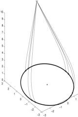
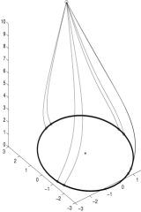
Figure 1: Schematic illustration of the method. Pairs of photons are emitted at slightly different proper times along the orbit, in precisely the right direction to reach the observer. Finding these photons is a boundary-value problem, and once found, each photon pair allows us to calculate the redshift at that point on the orbit by evaluating (5). At the left of the figure we have Minkowski photons, which move in straight lines. In the middle we have Schwarzschild photons, which are lensed. On the right, we have frame-dragged photons. The time difference between the emission of each photon in a pair has been exaggerated here for visual clarity. Note that it is only the star’s unrealistic proximity to the black hole that allows for such a visible depiction of the different effects.

Figure 1 is a schematic illustration of our method. Photons are emitted from nearby spacetime points on the stellar orbits and travel to the observer. In the left-hand picture, the star emits “Minkowski photons” which feel no space curvature and travel in straight lines; redshift depends only on the velocity and time dilation of the star. This is in effect the approximation used in previous work. In the middle picture, the star emits “Schwarzschild photons” which feel space curvature. In the right-hand picture, the star emits “frame dragging photons” which feel spin as well as space curvature.

Below, § 2.1 details the problem to be solved and the method used for calculation of the redshift. The Matlab scripts implementing our algorithm are available as an online supplement. Then § 2.2 presents the black-hole model and associated metrics which we use in our approach, and § 2.4 derives how the various effects scale with orbit size. We apply our algorithm to the star S2, and detail the results in Section 3.

2 The redshift-calculation method

2.1 A boundary-value problem

In order to calculate the redshift of a moving star as observed by a fixed observer, we need to solve the geodesic equations for both the star and for photons. Geodesic equations are commonly expressed in terms of the Lagrangian,

$$\mathcal{L}=\hbox{$\frac{1}{2}$}g_{\mu\nu}\dot{x}^{\mu}\dot{x}^{\nu}$$ (2)

with dots denoting derivatives with respect to the affine parameter. But an equivalent formulation exists in terms of a Hamiltonian

$$\mathcal{H}=\hbox{$\frac{1}{2}$}g^{\mu\nu}p_{\mu}p_{\nu}.$$ (3)

We will follow the latter in this work. Numerically $\mathcal{H}=\mathcal{L}$. We will in fact employ two Hamiltonians $\mathcal{H}_{\textrm{star}}$ and $\mathcal{H}^{\textrm{\thinspace null}}$, which are really two different approximations for the same Hamiltonian. Numerically $\mathcal{H}^{\textrm{\thinspace null}}=0$ of course. We will write $\lambda$ for the affine parameter of the star, and $\sigma$ for that of a photon.

Consider two photon trajectories, emitted at two points on the star’s orbit $\Delta\lambda$ apart in the affine parameter, with both photons terminating at the observer and arriving at time $\Delta t$ apart in the observer’s frame. Since $d\tau=\sqrt{|g_{\mu\nu}dx^{\mu}dx^{\nu}|}$, we are able to express the proper time between the emission events in terms of the affine parameter as

$$\Delta\tau=\Delta\lambda\sqrt{|2\mathcal{H}_{\textrm{star}}|}$$ (4)

where $\mathcal{H}_{\textrm{star}}$ is evaluated at either point of emission. Comparing with the definition (1) of the redshift, we have

$$z=\frac{\Delta t}{\Delta\lambda\sqrt{|2\mathcal{H}_{\textrm{star}}|}}-1.$$ (5)

We now need to compute $\Delta t$ for a given $\Delta\lambda$. To do this, we begin by calculating the orbit of the star for some chosen initial conditions, by solving Hamilton’s equations for $\mathcal{H}_{\textrm{star}}$ with $\lambda$ as the independent variable. The temporal component of the generalized momentum is set at $p_{t}=-1$. This amounts to choosing the units for $\lambda$ such that $dt=d\lambda$ outside of gravitational fields. We then choose a point on the star’s orbit whose observed redshift we wish to calculate, and from this point we seek a photon that will reach the observer.

Consider a function $\Phi^{j}$, which effectively shoots a photon by integrating Hamilton’s equations for $\mathcal{H}^{\textrm{\thinspace null}}$ with given initial conditions at affine parameter $\sigma=0$ and returns the 3-position at $\sigma=1$. We write

$$\Phi^{j}\left(t,x^{i},p_{i}\right)=x^{j}|_{\sigma=1}$$ (6)

where $i,j=1,2,3$ and the initial $p_{t}$ is chosen such that $\mathcal{H}^{\textrm{\thinspace null}}=0$. We pass the function $\Phi^{j}$ to a root-finder, and solve for the root of

$$f\left(p_{i}\right)=\Phi^{j}-x^{j}_{\textrm{obs}}$$ (7)

by varying the initial 3-momentum $p_{i}$. Naturally, we may not adjust the $x^{i}$, as we are interested in a specific point on the star’s orbit.

The root-finding algorithm requires a set of initial guesses for the initial $p_{i}$ of the photon. On this account, we shoot an initial-guess photon from the star position in the direction of the observer, that is, we evaluate $\Phi^{j}$ with trivial initial conditions. These initial-guess values for the $p_{i}$ shoot in the direction of the observer ignoring curvature. However, because the spacetime is indeed curved, this photon will not hit the observer. It serves only to start the root-finding algorithm.

Once the root-finder reports a solution within specified tolerance level, we move the star a very short distance ($\Delta\lambda$ in affine parameter) along its orbit, and repeat the above procedure, now solving for the sought-after trajectory at the star’s new position. The difference in arrival times of the two photons is $\Delta t$, which we insert into (5) to evalate the redshift.

Thus far we have solved for two photon trajectories. This computation has enabled us to calculate the redshift at a chosen point on the orbit. We may then repeat this process at further points along the orbit, garnering results as much as the required resolution demands.

2.2 Post-Newtonian and post-Minkowskian approximations

The spacetime outside a spinning black hole is described by the Kerr metric. Since the Galactic-center stars are far from the horizon, approximations valid only at large $r$ can be used to study general relativistic effects. Accordingly, we first derive two perturbative Hamiltonians, a post-Newtonian $\mathcal{H}_{\textrm{star}}$ for stars, and a post-Minkowskian approximation $\mathcal{H}^{\textrm{\thinspace null}}$ for photons. Different physical effects come into play at different orders of the perturbation parameter $\epsilon$, and we will show these numerically by toggling different terms on and off.

Taking the Kerr metric in Boyer-Lindquist coordinates with geometric units $GM=c=1$ (leaving us with a unit of length equal to the gravitational radius $GM/c^{2}\simeq 5\times 10^{6}$ km for the Galactic-center black hole) we have the full Hamiltonian

$$\mathcal{H}_{\textrm{Kerr}} = \frac{\left(r^{2}+s^{2}\right)^{2}-s^{2}\Delta\sin^{2}\theta}{2\rho^{2}\Delta}p_{t}^{2}-\frac{\Delta}{2\rho^{2}}p_{r}^{2}-\frac{1}{2\rho^{2}}p_{\theta}^{2}$$ (8)

$$-\frac{\Delta-s^{2}\sin^{2}\theta}{2\Delta\rho^{2}\sin^{2}\theta}p_{\phi}^{2}+\frac{2sr}{2\rho^{2}\Delta}p_{t}p_{\phi}$$

where

$$\Delta\equiv r^{2}-2r+s^{2}\quad\textrm{and}\quad\rho^{2}\equiv r^{2}+s^{2}\cos^{2}\theta.$$ (10)

and $s$ denotes the black hole spin parameter.

Let us first consider the dynamics of the star. Sufficiently far from the black hole, the post-Newtonian approximation

$$v^{2}\sim 1/r$$ (11)

applies. If we choose $v\sim\mathcal{O}\left(\epsilon\right)$ then by (11) $r$ is $\mathcal{O}\left(\epsilon^{-2}\right)$. Correspondingly, we force the velocity terms $p_{r}$, $p_{\theta}/r$ and $p_{\phi}/r$ to be $\mathcal{O}\left(\epsilon\right)$. Making the following replacements in (8)

$$r\rightarrow\epsilon^{-2}r,\quad p_{r}\rightarrow\epsilon p_{r},\quad p_{\theta}\rightarrow\epsilon^{-1}p_{\theta}\quad\mathrm{and}\quad p_{\phi}\rightarrow\epsilon^{-1}p_{\phi}$$ (12)

and keeping terms to $\mathcal{O}\left(\epsilon^{5}\right)$, we obtain

$$\mathcal{H}_{star}=-\frac{p_{t}^{2}}{2}+\left(\frac{p_{r}^{2}}{2}+\frac{p_{\theta}^{2}}{2r^{2}}+\frac{p_{\phi}^{2}}{2r^{2}\sin^{2}\theta}-\frac{p_{t}^{2}}{r}\right)\epsilon^{2}-\left(\frac{2p_{t}^{2}}{r^{2}}+\frac{p_{r}^{2}}{r}\right)\epsilon^{4}-\frac{2sp_{t}p_{\phi}}{r^{3}}\,\epsilon^{5}.$$ (13)

We can abbreviate (13) as

$$\mathcal{H}_{\textrm{star}}=\mathcal{H}_{\textrm{static}}+\epsilon^{2}\,\mathcal{H}_{\textrm{Kep}}+\epsilon^{4}\,\mathcal{H}_{\textrm{Schw}}+\epsilon^{5}\,\mathcal{H}_{\textrm{FD}}.$$ (14)

Here $\mathcal{H}_{\textrm{static}}$ produces motionless geodesics, $\mathcal{H}_{\textrm{Kep}}$ gives the Keplerian phenomenology, $\mathcal{H}_{\textrm{Schw}}$ is the weak-field Schwarzschild contribution that produces pericenter precession, while the angular-temporal term $\mathcal{H}_{\textrm{FD}}$ produces the Lens-Thirring effect or frame dragging.

Continuing now to photon trajectories, we remark that by the equivalence principle, the full Hamiltonian is exactly the same for photons and stars. However, the same terms can have different orders in the two regimes, prompting approximation $\mathcal{H}^{\textrm{\thinspace null}}$. In particular, the approximation (11) obviously does not hold for photons, which have $v^{2}=1$, implying the scalings

$$r\rightarrow\epsilon^{-2}r,\quad p_{\theta}\rightarrow\epsilon^{-2}p_{\theta}\quad\mathrm{and}\quad p_{\phi}\rightarrow\epsilon^{-2}p_{\phi}$$ (15)

with $p_{r}$ being $\mathcal{O}(1)$. Expanding as before, we obtain

$$\mathcal{H}^{\textrm{\thinspace null}}= -\frac{p_{t}^{2}}{2}+\frac{p_{r}^{2}}{2}+\frac{p_{\theta}^{2}}{2r^{2}}+\frac{p_{\phi}^{2}}{2r^{2}\sin^{2}\theta}-\left(\frac{p_{t}^{2}}{r}+\frac{p_{r}^{2}}{r}\right)\epsilon^{2}+$$

$$-\left(\frac{2p_{t}^{2}}{r^{2}}+\frac{2sp_{t}p_{\phi}}{r^{3}}-\frac{s^{2}\sin^{2}\theta}{2r^{2}}p_{r}^{2}+\frac{s^{2}\cos^{2}\theta}{2r^{4}}p_{\theta}^{2}\right)\epsilon^{4}$$ (16)

- a different selection of terms compared to the post-Newtonian case. There is no term at $\mathcal{O}(\epsilon^{5})$. We may abbreviate (16) as

$$\mathcal{H}^{\textrm{\thinspace null}}=\mathcal{H}^{\textrm{Mink}}+\epsilon^{2}\,\mathcal{H}^{\textrm{S${}_{\hbox{\tiny{LO}}}$}}+\epsilon^{4}\left(\mathcal{H}^{\textrm{S${}_{\hbox{\tiny{NLO}}}$}}+\mathcal{H}^{\textrm{FD}}+\mathcal{H}^{\textrm{torq}}\right).$$ (17)

At zeroth order we have special relativistic or Minkowski photons. The leading order Schwarzschild effect $\mathcal{H}^{\textrm{S${}_{\hbox{\tiny{LO}}}$}}$ gives the gravitational deflection of light. At $\mathcal{O}\left(\epsilon^{4}\right)$, however, there are three distinct effects: first $\mathcal{H}^{\textrm{S${}_{\hbox{\tiny{NLO}}}$}}$ gives a next-to-leading order correction to the Schwarzschild effect, the off-diagonal term $\mathcal{H}^{\textrm{FD}}$ gives frame dragging again but for photon trajectories, while $\mathcal{H}^{\textrm{torq}}$ provides a torque proportional to $s^{2}$.

2.3 Pseudo-cartesian coordinates

The spatial Boyer-Lindquist coordinates $r,\theta,\phi$ are convenient for computing stellar orbits, but not well suited for photon paths. The photon paths are nearly straight lines, but since the observer is much further from the black hole than the source, tiny variations in $\theta$ and $\phi$ at the observer imply large distances. As a result, both the integrator and the root-finder become susceptible to roundoff error.

To cure the problem, we change to pseudo cartesian coordinates. They are not purely cartesian, as the surface $x^{2}+y^{2}+z^{2}$ is not spherical.

$$x=r\sin\theta\cos\phi,\quad y=r\sin\theta\cos\phi,\quad z=r\cos\theta$$ (18)

The corresponding momenta are readily derived by completing the canonical transformation, leading to the usual relations

$$p_{r}=\frac{\textbf{x}\cdot\textbf{p}}{r},\quad p_{\phi}=\left(\textbf{x}\times\textbf{p}\right)_{z},\quad p_{r}^{2}+\frac{p_{\theta}^{2}}{r^{2}}+\frac{p_{\phi}^{2}}{r^{2}\sin^{2}\theta}=\textbf{p}^{2}.$$ (19)

The form of $\mathcal{H}^{\textrm{\thinspace null}}$ changes accordingly. The Minkowski part bears the familiar form

$$\mathcal{H}^{\textrm{Mink}}=-\frac{p_{t}^{2}}{2}+\frac{\textbf{p}^{2}}{2}.$$ (20)

The leading-order Schwarzschild terms are

$$\mathcal{H}^{\textrm{S${}_{\hbox{\tiny{LO}}}$}}=-\frac{p_{t}^{2}}{r}-\frac{\left(\textbf{x}\cdot\textbf{p}\right)^{2}}{r^{3}},$$ (21)

and the associated $\mathcal{O}(\epsilon^{4})$ term retains its previous form of

$$\mathcal{H}^{\textrm{S${}_{\hbox{\tiny{NLO}}}$}}=-\frac{2p_{t}^{2}}{r^{2}}.$$ (22)

Also at $\mathcal{O}(\epsilon^{4})$ we have the frame-dragging term

$$\mathcal{H}^{\textrm{FD}}=-\frac{2sp_{t}}{r^{3}}\left(\textbf{x}\times\textbf{p}\right)_{z},$$ (23)

and the torquing terms

$$\mathcal{H}^{\textrm{torq}}=\frac{s^{2}}{2r^{2}}\left(1-\frac{z^{2}}{r^{2}}\right)\left(\frac{\textbf{x}\cdot\textbf{p}}{r}\right)^{2}-\frac{s^{2}}{2z^{2}}\left[\textbf{p}^{2}-\left(\frac{\textbf{x}\cdot\textbf{p}}{r}\right)^{2}-\frac{\left(\textbf{x}\times\textbf{p}\right)^{2}_{z}}{r^{2}-z^{2}}\right].$$ (24)

The torquing terms are the most difficult to integrate numerically. This is because while the terms themselves are at $\mathcal{O}\left(\epsilon^{4}\right)$, they involve quotients of particularly high powers. Taking derivatives of $\mathcal{H}^{\textrm{torq}}$ further bloats these bottom and top heavy fractions, and provokes roundoff errors. We argue below that the torquing terms are in any case unimportant for the known Galactic-center stars. Hence we omit these terms in our numerical work.

2.4 Scaling properties of redshift contributions

We can infer the scaling with orbital size $a$ of the redshift contributions $\Delta z$ of the various perturbative terms in $\mathcal{H}_{\textrm{star}}$ with the following deliberation. Consider a perturbative term

$$\Delta\mathcal{H}_{\textrm{star}}\sim a^{-n}$$ (25)

Since $\mathcal{H}_{\textrm{star}}$ is constant along the orbit, any variation in $\Delta\mathcal{H}_{\textrm{star}}$ has to be balanced by a variation in the unperturbed Hamiltonian. Since the latter scales as $\mathcal{H}_{\textrm{star}}\sim 1/a$, we have $\Delta\mathcal{H}_{star}\sim\Delta a/a^{2}$, giving

$$\Delta a\sim a^{2-n}$$ (26)

Furthermore, since the orbital velocity scales as $v\sim a^{-1/2}$, we have $\Delta v\sim a^{-3/2}\,\Delta a$ and hence the redshift signal

$$\Delta z\left(\Delta H_{\textrm{star}}\right)\sim a^{\frac{1}{2}-n}.$$ (27)

A similar argument can be made for the perturbative terms $\Delta\mathcal{H}^{\textrm{\thinspace null}}$. In this case we compare photons emitted from the same point, only with different Hamiltonians. While the redshift signal from the previous case necessitated our consideration of the stellar velocity only, in analyzing the gravitational redshift signal, we are naturally interested in the time difference $\Delta t$ due to $\Delta H$. Let the perturbation be

$$\Delta\mathcal{H}^{\textrm{\thinspace null}}\sim r^{-n}.$$ (28)

Since the light travel time is an integrated quantity, we expect the change in the light travel time to scale as

$$\Delta t_{\textrm{trav}}\sim r^{1-n}$$ (29)

The change $\Delta t_{\textrm{trav}}$ in light travel time must not be confused with the difference $\Delta t$ in arrival time of two photons. For the latter quantity we get $\Delta t\sim\Delta r/r^{n}$ and since $\Delta r$ between two photons is $\sim v\sim a^{-1/2}$ we derive

$$\Delta z\left(\Delta\mathcal{H}^{\textrm{\thinspace null}}\right)\sim a^{-\frac{1}{2}-n}.$$ (30)

Using (27) and (30) and recalling that each power of $\epsilon$ in the Hamiltonians represents a scaling factor of $r^{-1/2}$ we can read off the following scalings.

$$\left(\begin{array}[]{ccc}&\mathcal{H}_{\textrm{Schw}}\\ &\mathcal{H}_{\textrm{FD}}\\ &\mathcal{H}^{\textrm{S${}_{\hbox{\tiny{LO}}}$}}\\ \mathcal{H}^{\textrm{S${}_{\hbox{\tiny{NLO}}}$}}&\mathcal{H}^{\textrm{torq}}&\mathcal{H}^{\textrm{FD}}\end{array}\right)\Rightarrow\Delta z\propto\left(\begin{array}[]{l}a^{-3/2}\\ a^{-2}\\ a^{-3/2}\\ a^{-5/2}\end{array}\right)$$ (31)

3 Application to S2-like orbits

We select S2 for a case study, since S2 has the shortest orbit and one of the highest pericenter velocities of all the known stars orbiting Sagittarius A^∗, and hence provides us with perhaps the best opportunity to observe general-relativistic effects.

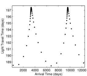
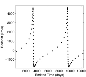
Figure 2: A redshift calculation for an S2-like star over two orbits. The left panel shows the time each photon takes to travel from the star to the observer. The star begins at apocenter, which happens to be closer to the observer than the pericenter. Therefore the light travel time naturally increases as the star moves towards its pericenter. The right panel shows the redshift. The peaks occur during pericenter passage due to the high pericenter passage velocities. The calculation includes post-Newtonian and post-Minkowskian effects, but these are too small to see in this figure.

Figure 2 shows a redshift calculation for a star with S2’s orbital parameters. These are taken from Gillessen et al. (2009). The gravitational radius is taken as $5\times 10^{6}\;\rm km$. For definiteness, we take the spin to be maximal, and pointing towards Galactic North. Disc seismology models (Kato et al., 2009) put the spin at $s\approx 0.44$. The direction however, remains unknown.

All the contributions to $\mathcal{H}_{\textrm{star}}$ in (14) are included for the orbit calculation. The photon trajectories include all contributions to $\mathcal{H}^{\textrm{\thinspace null}}$ in (17) except for $\mathcal{H}^{\textrm{torq}}$.

Naturally we would like to compute the redshift contributions of the various relativistic terms, and verify that they follow the expected scalings (31). In order to do this, we examine the differences between redshifts computed from different post-Newtonian and post-Minkowskian cases. This allows us to isolate the effects of $\mathcal{H}_{\textrm{Schw}},$ $\mathcal{H}_{\textrm{FD}},$ $\mathcal{H}^{\textrm{S${}_{\hbox{\tiny{LO}}}$}}$ and $\mathcal{H}^{\textrm{S${}_{\hbox{\tiny{NLO}}}$}}+\mathcal{H}^{\textrm{FD}}$, as follows.

1. To isolate $\mathcal{H}_{\textrm{Schw}}$ we compute the redshift difference $z_{\textrm{Schw}}^{\textrm{Mink}}-z_{\textrm{Kep}}^{\textrm{Mink}}$. By $z_{\textrm{Schw}}^{\textrm{Mink}}$ we mean that the star is followed using terms in $\mathcal{H}_{\textrm{star}}$ up to $\mathcal{H}_{\textrm{Schw}}$ and the photons are followed using $\mathcal{H}^{\textrm{\thinspace null}}$ up to $\mathcal{H}^{\textrm{Mink}}$. The same naming convention applies to $z_{\textrm{Kep}}^{\textrm{Mink}}$ and to other expressions of this type below.

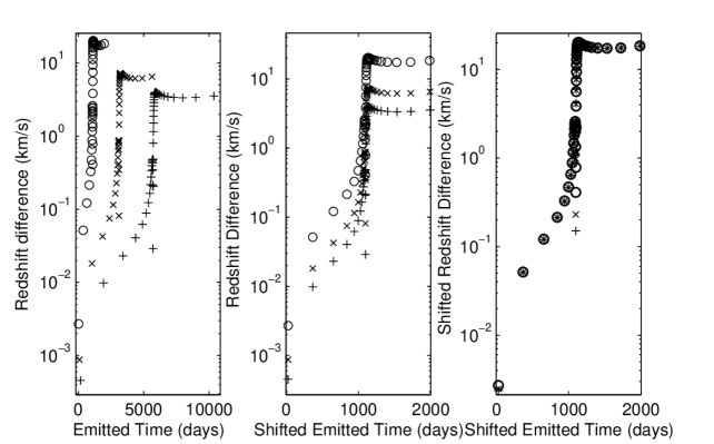
Figure 3: Redshift difference $z^{\textrm{Mink}}_{\textrm{Schw}}-z^{\textrm{Mink}}_{\textrm{Kep}}$ showing the contribution of $\mathcal{H}_{\textrm{Schw}}$. The left panel shows the redshift difference for three orbits, one with the parameters of S2, and the other two with $a$ doubled or halved. In the middle panel, the horizontal scale is stretched $(a/a_{\textrm{S2}})^{-3/2}$. In the right panel the redshift difference is scaled by $(a/a_{\textrm{S2}})^{-3/2}$.

   Figure 3 shows the redshift difference, calculated for three orbits going from apocenter to apocenter. One orbit has the parameters of S2; the two others have $a=2a_{\textrm{S2}}$ and $\hbox{$\frac{1}{2}$}a_{\textrm{S2}}$ with the other orbital parameters being the same. The redshift difference increases till pericenter and then declines somewhat, but not to its previous apocentric value, because the relativistic orbit experiences prograde Schwarzschild precession whereas the Keplerian orbit does not, and the resulting phase change in the orbit gives an increasing contribution to the redshift.

   For S2 parameters, the maximum redshift contribution of $\mathcal{H}_{\textrm{Schw}}$ is found to to be $\simeq 7\rm\,km\;s^{-1}$. For the other two stars, upon rescaling the redshift differences by $(a/a_{\textrm{S2}})^{-3/2}$ and the orbital time also by $(a/a_{\textrm{S2}})^{-3/2}$, the results can be overlaid almost perfectly on those of the S2-like star.

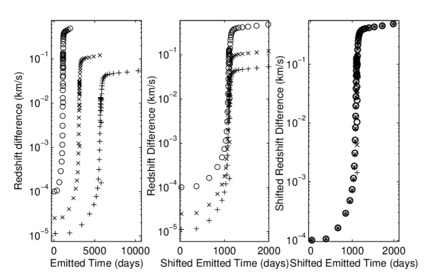
Figure 4: Redshift difference $z^{\textrm{Mink}}_{\textrm{FD}}-z^{\textrm{Mink}}_{\textrm{Schw}}$ showing the contribution of $\mathcal{H}_{\textrm{FD}}$. The scheme follows Figure 3 except that the redshift difference is scaled by $(a/a_{\textrm{S2}})^{-2}$.

2. To isolate $\mathcal{H}_{\textrm{FD}}$ we then compute the redshift difference $z_{\textrm{FD}}^{\textrm{Mink}}-z_{\textrm{Schw}}^{\textrm{Mink}}$. For an S2-like orbit the signal is around $0.1\rm\,km\;s^{-1}$ at pericenter, and as Figure 4 shows, the signal scales as $a^{-2}$.

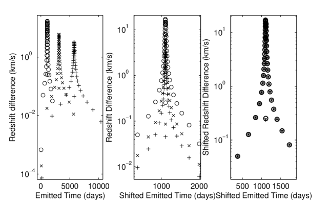
Figure 5: Redshift difference $z^{\textrm{S${}_{\hbox{\tiny{LO}}}$}}_{\textrm{Schw}}-z^{\textrm{Mink}}_{\textrm{Schw}}$ showing the contribution of $\mathcal{H}^{\textrm{S${}_{\hbox{\tiny{LO}}}$}}$. The scheme follows Figure 3, the redshift difference being scaled again $(a/a_{\textrm{S2}})^{-3/2}$.

3. To isolate $\mathcal{H}^{\textrm{S${}_{\hbox{\tiny{LO}}}$}}$ we compute $z^{\textrm{S${}_{\hbox{\tiny{LO}}}$}}_{\textrm{Schw}}-z^{\textrm{Mink}}_{\textrm{Schw}}$ and illustrate this difference in Figure 5. There is no precession-related redshift effect involved, because the photon types being compared refer to the same stellar orbits. The signal scales as $a^{-3/2}$ and for the S2-like orbit the maximum is $\simeq 2\rm\,km\;s^{-1}$.

   We see that the Schwarzschild terms in the stellar orbit and in the light path give comparable contributions to the redshift. To detect the Schwarzschild effect, it is necessary to take both into account.

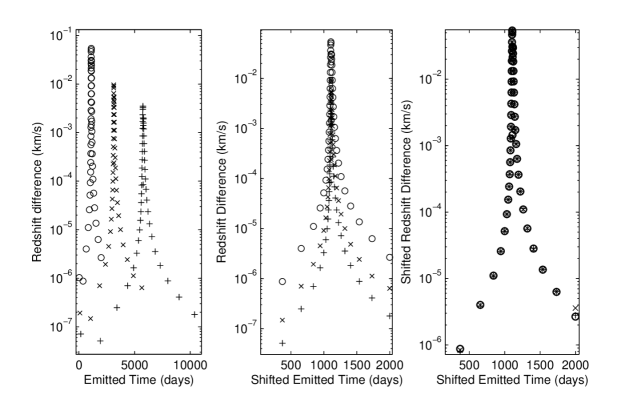
Figure 6: Redshift difference $z^{\textrm{FD}}_{\textrm{FD}}-z^{\textrm{S${}_{\hbox{\tiny{LO}}}$}}_{\textrm{FD}}$ showing the contribution of $\mathcal{H}^{\textrm{S${}_{\hbox{\tiny{NLO}}}$}}+\mathcal{H}^{\textrm{FD}}$. The scheme follows Figures 3–5, with the redshift difference scaled by $(a/a_{\textrm{S2}})^{-5/2}$. Here we have taken the spin as maximal, $s=1$. This signal is exactly proportional to s.

4. Finally, we isolate $\mathcal{H}^{\textrm{S${}_{\hbox{\tiny{NLO}}}$}}+\mathcal{H}^{\textrm{FD}}$ by computing $z_{\textrm{FD}}^{\textrm{FD}}-z_{\textrm{FD}}^{\textrm{S${}_{\hbox{\tiny{LO}}}$}}$. Figure 6 verifies the expected $a^{-5/2}$ scaling and shows that the maximum signal for S2 parameters is $\sim 10^{-2}\rm\,km\;s^{-1}$. Thus we see that the frame-dragging on photons is much smaller than on stars. Similarly, $\mathcal{H}^{\textrm{S${}_{\hbox{\tiny{NLO}}}$}}$ makes a much smaller contribution than $\mathcal{H}_{\textrm{FD}}$. We expect the contribution of $\mathcal{H}^{\textrm{torq}}$ would be similarly small, though we have not calculated it.

   We see that in order to measure the leading-order frame-dragging effect on Galactic-center stars, it is sufficient to consider Schwarzschild photons.

Of course, the computation method for weak redshift signals contains numerical errors, especially for higher-order effects being evaluated at large distances from the black hole. The numerical noise in our implementation drowns out the the leading-order Schwarzschild effect for scaled S2-like orbits with $a\approx 3\cdot 10^{8}$ — at which point the pericenter redshift signal is $\approx 5\cdot 10^{-6}\rm\,km\;s^{-1}$. Numerical noise would overwhelm the frame-dragging signal for scaled S2-like orbits with at $a\approx 1.2\cdot 10^{5}$. This being an order of magnitude larger than $a_{S2}$, and so we are in good shape to calculate the frame-dragging redshift contribution. For redshift signal contributions beyond those of frame-dragging, the numerical noise in our Matlab implementation of the algorithm is intolerable for $a_{S2}$. Were we calculating these effects for stars closer to the SBH, the higher-order signals would be stronger, and therefore less prone to round-off. In summary, for the known Galactic-center stars, the numerical noise in calculating relativistic redshifts will be well within the observational errors, even with the next generation spectral instrumentation.

4 Summary and Outlook

Some stars in orbit around the Galactic-center black hole reach velocities of a few percent light at pericenter, and the time-varying redshift of these stars during pericenter passage has small but distinctive perturbations from general relativity.

The redshift is dominated by the line of sight velocity, which for the star S2 reaches $v\sim 5\times 10^{3}\rm\,km\;s^{-1}$ at pericenter. The leading perturbations are from time dilation because (a) the star is moving, and (b) because it is in a potential well. Both of these make $\mathcal{O}(\beta^{2})$ contributions to the redshift (where $v$ is the stellar velocity in light units) and are well understood (Zucker et al., 2006). In this paper we have calculated additional perturbations from general relativity, which are the following.

1. The weak-field Schwarzschild effect on the stellar orbit, which contributes to redshift at $\mathcal{O}(\beta^{3})$. For S2 it is $\simeq 7\rm\,km\;s^{-1}$.

2. The frame-dragging effect of black hole spin on the stellar orbit, which perturbs the redshift at $\mathcal{O}(\beta^{4})$. For S2 it would be $\sim 10^{-1}\rm\,km\;s^{-1}$ for maximal spin.

3. The weak-field Schwarzschild effect on the light travelling from the star to us, which gives a redshift perturbation at $\mathcal{O}(\beta^{3})$. For S2 it is $\simeq 2\rm\,km\;s^{-1}$.

4. Frame dragging plus next-order Schwarzschild perturbation of the photon paths. These contribute at $\mathcal{O}(\beta^{5})$ to the redshift, and we estimate these as $\sim 10^{-2}\rm\,km\;s^{-1}$ for S2.

Of these, the first two are orbital effects and have been considered in previous work (Kannan & Saha, 2008; Preto & Saha, 2009). The last two are light-path effects, known about but not previously computed in the context of Galactic-center stars.

Clearly, in order to measure the Schwarzschild effects via the redshift, the effects of general relativity on both the stellar orbit and the light path must be computed, as they are of the same order. On the other hand, to leading order, frame dragging needs to be considered only in the orbit and can be neglected in the light path.

In order to test for the the presence and form of the NLO and NNLO terms in the metric, the calculated redshift curve must be fitted to the spectral data via a range of parameters. These include the orbital parameters and the black hole mass. In keeping these parameters variable, we can expect a requirement for spectroscopic accuracy less than the signal sizes themselves. Bear in mind however, that this depends on the number of data points. The inclusion of astrometric data to the fitting procedure will help relax the accuracy bound.

Observationally, the Galactic-center stars are of course observable only in infrared. For the most massive stars, including S2, the Brackett-$\gamma$ line at $2.16\,\mu\rm m$ is the most prominent available spectral feature, and has an intrinsic dispersion of $\sim 100\rm\,km\;s^{-1}$ (see e.g., Martins et al., 2008). For low-mass stars, the edges of the CO molecular bands (the so-called CO band heads) are excellent sharp features for redshift measurements.

The SINFONI spectrograph, an instrument at the VLT, has a spectral resolution of $75\rm\,km\;s^{-1}$. Redshift errors are currently estimated at 10s of $\rm\,km\;s^{-1}$ (see Section 4.1 of Gillessen et al., 2009) but expected to improve. Measurements by this instrument during S2’s next pericenter passage in 2016 could suffice to provide data from which the Schwarzschild signals could be extracted.

Spectral measurements seeking the spin-dependent signals are far beyond the capabilities of existing infrared spectrographs. On the other hand, recent developments such as laser-comb spectrographs (see e.g., Steinmetz et al., 2008) suggest optimism that the spectral resolutions of next-generation instruments will prove adequate.

Meanwhile, there are some theoretical issues that require further research.

• Given a model of gravity which is metric, and an associated energy-momentum distribution, for which we have a metric, we are able to calculate the general relativistic redshift as observed by the Earth. Should we wish to probe the agreement of measured redshift contributions with a model, an effective way of working backwards needs to be formulated. Given redshift curve data of sufficient resolution, methods for determining the model from such must be developed.

• The Kerr Black Hole metric is a vacuum solution to the Einstein field equations. The assumption of a ‘clean’ metric is an oversimplification. An extended Newtonian mass distribution in the galactic center is anticipated. Accreting material, gas, and a possible accumulation of dark matter in the center could play a significant role in the dynamics. Such mass distributions need to be included in the metric.

• The possibility of a non-Einsteinian black hole metric should not be disregarded. Alternative theories of gravity possess black hole solutions whose phenomenology differs potentially already at low order (Will, 1993) from weak-field Einstein gravity. Suitable measurements, combined with the concession of extended mass distributions would allow for the identification of potentially revealing redshift contributions. Conclusive results of such studies would likely require spectral measurements with a resolution beyond that offered by present-day generation instruments.

References

- Eisenhauer et al. (2009) Eisenhauer, F., Perrin, G., Brandner, W., Straubmeier, C., Bhm, A., Baumeister, H., Cassaing, F., Clnet, Y., Dodds-Eden, K., Eckart, A., Gendron, E., Genzel, R., Gillessen, S., Grter, A., Gueriau, C., Hamaus, N., Haubois, X., Haug, M., Henning, T., Hippler, S., Hofmann, R., Hormuth, F., Houairi, K., Kellner, S., Kervella, P., Klein, R., Kolmeder, J., Laun, W., Lna, P., Lenzen, R., Marteaud, M., Naranjo, V., Neumann, U., Paumard, T., Rabien, S., Ramos, J. R., Reess, J. M., Rohloff, R.-R., Rouan, D., Rousset, G., Ruyet, B., Sevin, A., Thiel, M., Ziegleder, J., & Ziegler, D., S. 2009, GRAVITY: Microarcsecond Astrometry and Deep Interferometric Imaging with the VLT
- Fragile & Mattews (2000) Fragile, P. C. & Mattews, G. J. 2000, The Astrophysical Journal, 542
- Ghez et al. (2008) Ghez, A., Weinberg, N., Lu, J., Do, T., Dunn, J., Matthews, K., Morris, M., Yelda, S., Becklin, E., Kremenek, T., Milosavljevic, M., & Naiman, J. 2008, The Astrophysical Journal, 689
- Gillessen et al. (2009) Gillessen, S., Eisenhauer, F., Trippe, S., Alexander, T., Genzel, R., Martins, F., , & Ott, T. 2009, The Astrophysical Journal, 692, 1075
- Jaroszynski (1998) Jaroszynski, M. 1998, Acta Astronomica, 653
- Kannan & Saha (2008) Kannan, R. & Saha, P. 2008, Astrophysical Journal 690 (2009) 1553-1557
- Kato et al. (2009) Kato, Y., Miyoshi, M., Takahashi, R., Negoro, H., & Matsumoto, R. 2009, ArXiv e-prints
- Martins et al. (2008) Martins, F., Gillessen, S., Eisenhauer, F., Genzel, R., Ott, T., & Trippe, S. 2008, ApJ, 672, L119
- Müller & Camenzind (2004) Müller, A. & Camenzind, M. 2004, A&A, 413, 861
- Preto & Saha (2009) Preto, M. & Saha, P. 2009, ApJ submitted and ArXiv 0906.2226
- Steinmetz et al. (2008) Steinmetz, T., Wilken, T., Araujo-Hauck, C., Holzwarth, R., Hänsch, T. W., Pasquini, L., Manescau, A., D’Odorico, S., Murphy, M. T., Kentischer, T., Schmidt, W., & Udem, T. 2008, Science, 321, 1335
- Will (1993) Will, C. M. 1993, Theory and experiment in gravitational physics REVISED EDITION (Cambridge University Press)
- Will (2008) Will, C. M. 2008, ApJ, 674, L25
- Zucker et al. (2006) Zucker, S., Alexander, T., Gillessen, S., Eisenhauer, F., & Genzel, R. 2006, The Astrophysical Journal Letters, 639, L21