Anharmonic contributions in real RF linear quadrupole traps

Abstract

The radiofrequency quadrupole linear ion trap is a widely used device in physics and chemistry. When used for trapping of large ion clouds, the presence of anharmonic terms in the radiofrequency potential limits the total number of stored ions. In this paper, we have studied the anharmonic content of the trapping potential for different implementations of a quadrupole trap, searching for the geometry best suited for the trapping of large ion clouds. This is done by calculating the potential of a real trap using SIMION8.0, followed by a fit, which allows us to obtain the evolution of anharmonic terms for a large part of the inner volume of the trap.

1 Introduction

The trapping of charged particles by radiofrequency (RF) electric fields was first demonstrated in 1954 [1] and quickly proved to be an extremely powerful tool for the experimental investigation of a wide range of phenomena. In particular the linear quadrupole RF trap is found at the heart of many experiments where few to many ions are laser-cooled to very low temperature for applications in optical frequency metrology [2], quantum computation  [3, 4] and formation of large Coulomb crystals [5]. In this paper, the deviation from the ideal harmonic potential is evaluated for different implementations of linear quadrupole ion traps, in order to maximize the number of trapped ions.

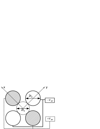
Figure 1: Schematic transverse view of a linear RF trap made of four cylindrical electrodes. The axes convention is shown, as well as the definitions of the applied RF voltages $V_{rf}=\frac{U_{0}+V_{0}\cos{\Omega t}}{2}$, the trap radius $r_{0}$ and the electrode radius $r_{e}$.

In this article, we briefly recall the basic information about linear quadrupole traps; detailed descriptions of RF traps and trajectories of the stored ions can be found in several textbooks (e.g. [6]). The most simple linear RF trap is formed by four parallel rods of radius $r_{e}$, see figure 1. In such devices, the trapping of charged particles in the transverse direction is achieved by applying an alternating potential difference between two pairs of electrodes (called the RF electrodes in the following). The trapping along the symmetry axis of the trap (to be taken as the $z$ axis) is realised by a static potential applied to two electrodes sets at both ends of the trap (called the DC electrodes in the following). The potential at the centre of a quadrupole linear trap is then well approximated by:

$$\phi(x,y,z,t) = \frac{(U_{0}+V_{0}\cos{\Omega t})}{2r^{2}_{0}\mathcal{L}}(x^{2}-y^{2})$$ (1)

$$+ \frac{\kappa U_{dc}}{z_{0}^{2}}\left(\frac{2z^{2}-x^{2}-y^{2}}{2}\right)$$

where $V_{0}$ is the amplitude of the RF potential difference between two neighbouring electrodes, $U_{0}$ a static contribution to this potential and $U_{dc}$ the voltage applied to the DC electrodes. $\Omega$ is the angular frequency of the RF voltage, $r_{0}$ is the inner radius of the trap, $2z_{0}$ is the length of the trap, corresponding to the distance between the DC electrodes, $\kappa$ and $\mathcal{L}$ are geometric loss factors. $\kappa$ is mainly induced by shielding effects whereas $\mathcal{L}$ stands for a loss in trapping efficiency due to the non-ideality of the quadrupole [7]. While in most cases $\phi$ is an accurate approximation close to the trap axis and around $z\simeq 0$, strong deviations occur further away from the center. The deviations induced depend strongly on the geometry used for the trap, as it is shown in the present article.

The motion of a single ion in a potential defined by $\phi(x,y,t)$ is described by the Mathieu differential equations [8]. The stability of the trajectory is controlled by the Mathieu parameters, which depend on the working parameters of the trap and on the charge ($Q$) and mass ($M$) of the particle:

$$q_{x}=-q_{y}=\frac{2QV_{0}}{M\Omega^{2}r_{0}^{2}\mathcal{L}}$$

$$a_{x}=a-\Delta a~{}~{}; a_{y}=-(a+\Delta a)$$ (2)

$$a=\frac{4QU_{0}}{M\Omega^{2}r_{0}^{2}\mathcal{L}}~{}; \Delta a=\frac{4\kappa QU_{dc}}{Mz_{0}^{2}\Omega^{2}}$$

where $a$ represents the Mathieu parameter of the pure quadrupole mass filter, and $\Delta a$ is the perturbation introduced by the presence of the axial confining voltage [9]. Most traps are operated in the adiabatic regime, where it is possible to decouple the short time scale of the RF driven motion, called micromotion, and the longer time scale of the motion induced by the envelope of the electric field, known as macromotion [10]. In this frame, the ion’s motion is the superposition of a periodic oscillation in an effective harmonic potential, characterized by the radial frequencies $\omega_{x}(a_{x},q_{x},\Omega)$ and $\omega_{y}(a_{y},q_{y},\Omega)$, with the RF-driven motion (at frequency $\Omega$) with an amplitude proportional to the local RF electric field.

The simultaneous trapping of two or more ions couples the $x$ and $y$ equations of motion through a nonlinear term induced by the Coulomb interaction and an analytical solution does not exist any longer. Moreover, due to this nonlinear contribution the ions gain energy from the RF field. This energy gain depends on the ion density and/or neutral background pressure inducing collisions [11]. While it can be negligible for very dilute ion clouds in good vacuum conditions, it can be a critical point for the storage of dense clouds where an important fraction of the ions can be lost due to this gain of energy.

Nevertheless, even in the case of a single ion in a perfect vacuum, nonlinearities can be introduced in the equations of motion by differences between the real RF and DC potentials and the ideal case. Imperfections in the potentials come from misalignments of the different electrodes and differences between the electrode surfaces from the ideal equipotential surfaces. These effects are very well known for hyperbolic Paul traps where holes in the electrodes are necessary for the injection and extraction of ions, electrons or light. Moreover, these undesired contributions to the potential can contain higher harmonic contributions which lead to a special form of RF-heating. More precisely, it has been shown [12] that for an imperfect Paul trap, nonlinear resonances leading to the loss of ions occur in the otherwise stable region, if the ion’s secular frequencies and the radiofrequency are related by a linear combination with integer coefficients ($N_{x},N_{z},k$):

$$N_{x}\omega_{x}+N_{z}\omega_{z}=k\Omega.$$ (3)

This resonant phenomena due to nonlinear couplings has been observed experimentally by several groups [13, 14].

Ideal harmonic potentials are obtained only if the shape of the RF electrodes follows the theoretical equipotential surface, a hyperbolic surface in the case of a quadrupole trap. The difficulty in machining such surfaces can be overcome by realizing circular rods. In this case, the relation $r_{e}=1.14511r_{0}$ between the trap radius $r_{0}$ and the electrode radius $r_{e}$ guarantees a minimal contribution of the lowest order term in the perturbation potential expansion for infinitely long RF electrodes [15]. This radius ratio is used for all the traps studied in this article. While some work has been done in optimizing miniature [7] and cylindrical [16] traps designs, to our knowledge no study has concentrated on the study of the anharmonic terms in a real linear trap.

Our research project aims at trapping a very large and laser-cooled ion cloud to study fundamental phenomena related to their dynamics and thermodynamics. In order to reach a very high temporal stability of the ion number, the trapping potential has to be quasi-ideal over a large part of the trapping volume. The ion cloud is expected to fill the trap to half the trap size in both directions ($-z_{0}/2<z<z_{0}/2$ and $0<r<r_{0}/2$) with a sufficiently high ion density such that a high number of ions ($\sim 10^{7}$) can be reached in a compact trap.

The present study evaluates the anharmonic contributions to the trapping potential of various existing devices and proposes an optimised alternative version. Contributions due to the finite size of the RF electrodes and to the shape of the DC electrodes are quantified and compared. Contrary to former studies in spherical traps [7] where anharmonic contributions were evaluated in the very centre of the trap ($r/r_{0},z/z_{0}<0.1$), which is relevant for single ions or chains of single ions, the present study is made in three dimensions and extends to values beyond $z_{0}/2$. This is motivated because a large ion cloud explores a much bigger volume of the trap, and therefore it is desirable that this volume has a low anharmonic content in order to minimise RF-heating.

Figure 2 shows the two geometries initially analysed. We have chosen only devices which leave the z-axis free as this axis is often needed to implement laser cooling and/or to introduce/extract ions. The segmented rod geometry (#1) is used, among others, by the Ion Trap Group in Åarhus University to trap large ion crystals [5, 9].

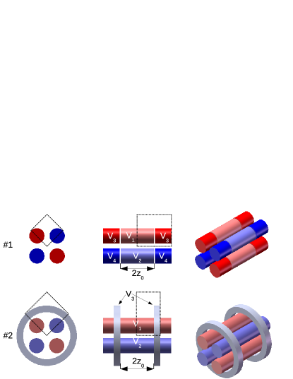
Figure 2: (Color Online) Design of the first two analysed geometries. The dimensions used in both cases are: $r_{0}=4$ mm and $z_{0}=10$ mm, with $r_{e}=1.14511r_{0}$. Trap #1 is formed by four segmented rods whose electrical connections are detailed in table 1. Trap #2 consists of four continuous rods surrounded by DC electrodes made of two external rings of longitudinal dimension $l_{ring}=4$ mm, inner radius $r_{int}=(r_{0}+2r_{e})+1$ mm and outer radius $r_{ext}=r_{int}+5$ mm. The distance between these rings defines $2z_{0}$. The dotted lines define the volume used for the SIMION8.0 calculations.

This geometry can be used with two different electrical configurations, named #1.1 and #1.2 (see table 1 for details). #1.2 has been analyzed due to its simplicity as #1.1 requires a much more advanced electronic configuration than #1.2 (see table 1). The second implementation, #2, is similar to one of the trap used in Quantum Optics and Spectroscopy Group at Innsbruck University for quantum information experiments [17].

Table 1: Electrical configuration for the different trap geometries.

	$V_{1}$	$V_{2}$	$V_{3}$	$V_{4}$
#1.1:	$+V_{rf}$	$-V_{rf}$	$U_{dc}+V_{rf}$	$U_{dc}-V_{rf}$
#1.2:	$+V_{rf}$	$-V_{rf}$	$U_{dc}$	$U_{dc}$
#2:	$+V_{rf}$	$-V_{rf}$	$U_{dc}$	–

This article is organised in several sections. The method used to calculate the potential created by a given geometry and the fitting procedure is described in section 2. In section 3, the anharmonic contributions are calculated and evaluated for the RF-part while we discuss the DC potential in section 4. Finally, an alternative geometry is introduced and analysed in section 5, followed by the conclusion, section 6.

2 Fitting the “real” trap potentials

2.1 Computation of the potentials

The commercial software SIMION8.0 [18] has been used to numerically solve the Laplace equation for each geometry. SIMION8.0 uses a Finite Difference Method (FDM), where the solution is obtained at each node of the mesh used to describe the electrodes and the space between them. The error on the electrostatic potential using FDM scales with $1/h$ [19], where $h$ is the node density (number of nodes/mm), but the reached accuracy depends on the particular geometry of the electrodes. In order to check the $1/h$ dependency and to obtain an estimation of the accuracy of the results given by the software, we have used SIMION8.0 to calculate the potential for infinitely long electrodes  with hyperbolic sections in which case the potential can be exactly described by: $\phi_{a}(x,y)=\frac{x^{2}-y^{2}}{2r_{0}^{2}}$ when $V_{0}=0$ and $U_{0}=1V$. Note that while the confinement is achieved dynamically, the anharmonic contributions to the potential do not depend on time and can be analysed as a static property of the trap.

We can then calculate the average relative error $Er(h)$, as a function of the node density $h$, using:

$$Er(h)=\frac{1}{n_{x}n_{y}}\sum_{i}^{n_{x}}\sum_{j\neq i}^{n_{y}}{\left|\frac{\phi_{s}(x_{i},y_{j})-\phi_{a}(x_{i},y_{j})}{\phi_{a}(x_{i},y_{j})}\right|},$$ (4)

where $\phi_{s}(x_{i},y_{j})$ is the SIMION8.0 solution with $x_{i+1}-x_{i}=y_{i+1}-y_{i}=h$ and $n_{x}$, $n_{y}$ are the number of nodes.

Figure 3 shows $Er(h)$ for $0\leq x\leq r_{0}/2$ and $0\leq y\leq r_{0}/2$ (the axes are oriented as in Fig 1). Fig 3 also shows a fit using $f(h)=a/h$. The comparison of the two plots indicates that $Er(h)$ closely follows the $1/h$ law. The error bars correspond to one standard deviation, $\sigma$.

For the computation of the potential created by #1 and #2, all possible symmetries have been used to reduce the required volume, as indicated in figure 2 by the dashed lines. This is important due to computer memory issues, which limit the mesh density which can be used for a given problem. In the present study, we were limited to a node density of 32 nodes/mm, for all computations carried out for a 3D volume. Figure 3 shows that this mesh density already provides an accuracy of 0.3 % for the hyperbolic trap. As the sizes of the studied traps are identical to the hyperbolic trap, the precision reached by SIMION8.0 is of the same order. Therefore, the use of the potentials computed by SIMION8.0 in the study of the anharmonic content in a quadrupole linear trap is fully justified.

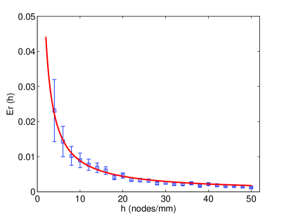
Figure 3: (Color Online) Estimation of the error between the numerical solution given by SIMION8.0 and the known analytical potential in the case of infinite hyperbolic electrodes as a function of the mesh density $h$. The dots show $E_{r}(h)$ calculated by equation 4 whereas the curve plots $f(h)=a/h$, with $a=8.8\times 10^{-2}$. The error bars correspond to $1\sigma$.

2.2 Fitting the potentials

An analytical two-dimensional solution of the Laplace equation for a quadrupole trap with circular sections exists, if we assume infinitely long RF electrodes [15]:

$$\phi(x,y)=C_{0}+Real\left\{\sum^{\infty}_{m=0}{C_{(4m+2)}\xi^{(4m+2)}}\right\};~{}~{}~{}~{}~{}~{}\xi=x+iy$$ (5)

where $C_{(4m+2)}$ are real coefficients and we have introduced a uniform contribution $C_{0}$ to equation (8) of [15].

As pointed out in the introduction, the term $C_{6}$ vanishes for infinitely long electrodes for $r_{e}=1.14511r_{0}$ [15]. To test our analysis of the potentials, we have computed the potential created by a 2D mass filter (infinitely long RF electrodes, without DC electrodes) for several values of the radius ratio $r_{e}/r_{0}$ and found the $C_{(4m+2)}$ coefficients of equation 5, by a fitting procedure analysed in the following. The evolution of $|C_{6}|$ as a function of $r_{e}/r_{0}$ shown in figure 4 shows that the $C_{6}$ term can be decreased by 3 orders of magnitude by choosing the appropriate radius ratio and confirms the zero crossing of $C_{6}$ for a $r_{e}/r_{0}$ value between $1.144$ and $1.146$. This accuracy corresponds to the maximal spatial resolution of our mesh for this problem (a high mesh density of 500 nodes/mm was possible due to the 2D nature of the problem). While this method does not provide a precise estimation of the “magic” radius ratio, it clearly agrees with the analytical result of $r_{e}=1.14511r_{0}$, showing that SIMION8.0 produces a very good representation of the potential created by an RF-trap. Higher order terms show a similar quantitative behavior as $C_{6}$, with respective minima for $C_{10}$ at $r_{e}/r_{0}\approx 0.78$, and $r_{e}/r_{0}\approx 0.58$ for $C_{14}$.

In addition, figure 4 shows the ratio between the ideal and the computed $C_{2}$ coefficients which corresponds to the geometrical loss factor, $\mathcal{L}$ introduced in equation 1:

$$\mathcal{L} = \frac{C_{2}^{ideal}}{C_{2}^{real}}$$ (6)

$$C_{2}^{ideal} = \frac{U_{0}}{2r^{2}_{0}}$$

For the chosen radius ratio, there is no loss of trapping efficiency induced by the circular shape of the electrodes ($\mathcal{L}\simeq 1$). We can observe that $\mathcal{L}$ takes values below 1 for larger electrode radius, which for experimental reasons (decreasing inter-electrode distance) might not be an appropriate choice. In the following, all the studied trap configurations have the same radius $r_{0}=4$ mm and $r_{e}=4.58$ mm.

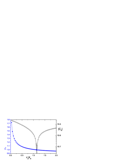
Figure 4: (Color Online) Squares and right axis: absolute value of the first anharmonic coefficient $C_{6}$, versus $r_{e}/r_{0}$ for $r_{0}=4$ mm. Blue circles and left axis: loss factor, $\mathcal{L}$ versus $r_{e}/r_{0}$.

The finite size of the rods and the presence of the DC electrodes introduce a dependency on $z$ of the coefficients $C_{(4m+2)}$. This dependency can be obtained by performing a fit at each node along $z$ to the numerical solution obtained by SIMION8.0. The trap parameters chosen are $V_{0}=0$, $U_{0}=1V$ and $U_{dc}=0$. These values remain the same throughout the paper, unless specified otherwise. A truncated version of eq.5 is used to perform a least-squares fit [20]. The points included in the fitting procedure belong to a 2D-square defined by $0\leq x\leq r_{0}/2$ and $0\leq y\leq r_{0}/2$, as $r=r_{0}/2$ is considered as the maximum expected radius of the trapped ion cloud.

To demonstrate the relevance of the fit, the $\chi^{2}$ of the fitting procedure for geometry #1.1 is plotted on figure 5 for each $z_{k}$ and for increasing maximum order $m_{max}$ included in the fitting equation (5).

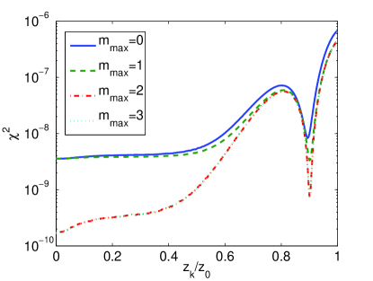
Figure 5: (Color Online) Evolution of the $\chi^{2}$ of the fitting procedure versus $z_{k}/z_{0}$, for increasing highest order $m_{max}$ included in the fitting equation 5. The curves corresponding to $m_{max}$ = 2 and 3 overlap each other, showing that no gain is obtained by retaining orders higher than $m_{max}=2$.

These curves illustrate several features. First, they confirm that the $C_{6}$ ($m=1$) contribution does not modify the quality of the fit in the center of the trap, which is expected from the choice of the electrode radius $r_{e}$ that nulls the $C_{6}$ contribution to the potential for infinitely long electrodes. Second, they demonstrate that adding higher orders than $m=2$ does not lead to an improvement of the fit and in the following $m=2$ is the highest order retained in the fitting function. Furthermore, the $\chi^{2}$ parameter, which is lower than $10^{-9}$ for $z_{k}\leq z_{0}/2$ and $m_{max}=2$ increases drastically from $z_{k}=z_{0}/2$ to $z_{0}$. From $z_{k}/z_{0}=0.6$, one can see that adding higher order terms to the fitting equation does not result in an improvement of the $\chi^{2}$ parameter. This means that equation (5) is not relevant in this part of the trap to reproduce the potential calculated by SIMION8.0 and that another analytical expression should be introduced to represent the potential close to the DC electrodes. As we are interested in fitting the potential for $z_{k}/z_{0}<0.5$, curves of figure 5 confirm the relevance of the fitting equation on the volume of interest.

To compare the precision of the fitting procedure to the precision of the SIMION8.0 calculation, we define the relative error of the fit, $Er_{fit}(z_{k})$, taken as the relative difference averaged over the transverse plane, between the SIMION8.0 solution, $\phi_{s}(x_{i},y_{j},z_{k})$, and the fitted potential, $\phi_{f}(x_{i},y_{j},z_{k})$:

$$Er_{fit}(z_{k})=\frac{1}{n_{x}n_{y}}\sum_{i}^{n_{x}}\sum_{j\neq i}^{n_{y}}{\left|\frac{\phi_{s}(x_{i},y_{j},z_{k})-\phi_{f}(x_{i},y_{j},z_{k})}{\phi_{s}(x_{i},y_{j},z_{k})}\right|}$$ (7)

The relative error $Er_{fit}(z_{k})$ is calculated for the geometry #1.1 and #2 for $z_{k}\leq z_{0}/2$. For this relative error, the addition of the $m=2$ contribution to the fitting potential allows reducing $Er_{fit}(z_{k})$ by a factor of 3 in the centre of the trap and by a factor of 2 at $z_{k}=z_{0}/2$. The relative error then reaches $5\times 10^{-6}$ in the center of the trap for both geometries and $8\times 10^{-6}$ for geometry #2 and $13\times 10^{-6}$ for geometry #1.1 at $z_{k}=z_{0}/2$. This relative error is three orders of magnitude smaller than the relative error one can expect from the SIMION8.0 calculations. Nevertheless, fitting the calculated potential is relevant for comparison between different geometries as the relative precision of the fit is as good for the two geometries considered in the text and the precision of the SIMION8.0 calculations should be identical as the basic geometry is the same for all the configurations compared here. Once all the coefficients $C_{4m+2}(z_{k})$ are determined at each $z_{k}$ and for each configuration, it is possible to study the evolution of the anharmonic contribution along the trap axis and to compare the different configurations.

3 Anharmonic contribution

The relative anharmonic contribution, $\zeta(x,y,z)$ of the potential in the trap can be obtained using:

$$\phi_{r}=\phi_{q}(1+\zeta+\Delta\zeta)$$ (8)

with

$$\phi_{q} = C_{0}+Real\{C_{2}\xi^{2}\}$$

$$\zeta = \frac{Real\{C_{6}\xi^{6}+C_{10}\xi^{10}\}+\Delta\phi_{f}}{C_{0}+Real\{C_{2}\xi^{2}\}}$$

$$\Delta\zeta = \frac{\Delta\phi_{s}}{C_{0}+Real\{C_{2}\xi^{2}\}}$$

where $\phi_{r}$ represents the real potential created by each geometry and $\phi_{q}$ its harmonic contribution. $\Delta\phi_{f}$ is the difference between the SIMION8.0 solution and the fitted potential calculated using the $C_{4m+2}(z_{k})$ coefficients found by the fitting algorithm. $\Delta\phi_{s}$ represents the unknown difference between the real and the SIMION8.0 solution, $\Delta\zeta$ is its relative value with respect to the harmonic contribution $\phi_{q}$.

In order to facilitate the visualisation of the behaviour of the anharmonic content, it is useful to calculate the averaged absolute value of $\zeta$ along the $z$-axis:

$$\langle\zeta(z_{k})\rangle=\frac{1}{n_{x}n_{y}}\sum_{i}^{n_{x}}\sum_{j}^{n_{y}}{\left|\zeta(x_{i},y_{j},z_{k})\right|}$$ (9)

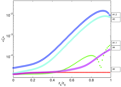
Figure 6: (Color Online) Averaged anharmonic contribution $\langle\zeta(z_{k})\rangle$ along the trap axis for the configurations #1.1, #1.2, #2. Configurations #3 and #4 are introduced later in the text. Strong differences between the trap configurations appear from $z_{k}/z_{0}>0.2$. For clarity, only every $4^{th}$ node is plotted.

The evolution of $\langle\zeta(z_{k})\rangle$ is shown in figure 6 for the configurations #1.1, #1.2 and #2. While all the configurations have comparable anharmonic content at the centre of the trap, strong differences appear between them when leaving the trap centre. As expected, due to the length of the RF electrodes with respect to the studied volume, configurations #1.1 and #2 show lower values of $\langle\zeta(z_{k})\rangle$ compared to #1.2. The increment observed from $z_{k}/z_{0}>0.5$ in the case of #1.1 can be explained by the unavoidable gap between RF and DC electrodes which generates a rise of the anharmonic content at the edge of the trap. The dip observed for $\langle\zeta_{\#1.1}(z_{k})\rangle$ is due to a zero crossing of the $\zeta(x_{i},y_{j},z_{k})$ in equation(9). In the area of interest $\langle\zeta(z_{k})\rangle$ remains rather constant along the trap axis for #2 and #1.1.

Figure 6 shows that the truncation of the RF electrodes in configuration #1.2 leads to a substantial increase of the anharmonicity from $z_{k}/z_{0}>0.3$, which could limit the usable trapping volume. To demonstrate the effect of the boundary conditions, we have calculated the potential created by a configuration called #3, similar to #1.2 but with the DC-rods removed. We observe in fig  6 that this leads to a reduction of the the anharmonic terms, illustrating the importance of geometric aspects.

We emphasize here that the only difference between #1.1 and #1.2 is in the voltage applied to the DC electrodes. Therefore, the discretization of the mesh by SIMION8.0 and so the calculation error is exactly the same for the two configurations. The fact that the expected behaviour of the anharmonic contribution is reproduced in each case re-enforces the validity of the assumption that SIMION8.0 error contribution is the same for all the configurations and that the comparative study performed in this article is significant.

4 DC-potentials

In this section, we focus on the potential created by the DC electrodes inside the trap, as it also strongly depends on the chosen configuration. While at the very centre of the trap, the potential can be approximated by an harmonic function, it is not necessarily true if larger volumes of the trap are considered. A harmonic potential shape can be desirable as it is often a necessary assumption when describing the ion dynamics or equilibrium properties inside the trap, as for example to calculate the aspect ratio (radius over length) of an ion cloud [21]. Figure 7 shows the potentials created only by the DC electrodes ($V_{0}=U_{0}=0$) of the geometries #1 and #2, along the z-axis. For comparison, these potentials have been normalised using:

$$V^{norm}_{DC}(x,y,z)=\frac{V_{DC}(x,y,z)-V_{DC}(0,0,0)}{V_{DC}(0,0,z_{0})-V_{DC}(0,0,0)}.$$ (10)

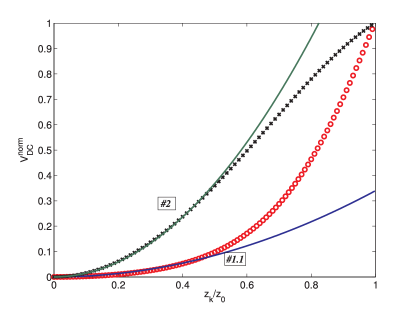
Figure 7: (Color Online) Normalised potentials created by the DC electrodes on axis (0,0,z) for geometries #1 (empty circles) and #2 (crosses) together with their respective fits to $f(z)=az^{2}$(solid lines). Notice that the fit was performed considering only $V(z_{k}\leq 0.5z_{0})$.

A fit to $f(z)=az^{2}$ using only the values of the potential in the interval $0\leq z_{k}/z_{0}\leq 0.5$ (see fig 7) clearly shows the divergence from an harmonic potential at the outer edges of the trap. In order to quantify the degree of harmonicity, we successively extended the fit, starting from the centre, until the correlation coefficient $R^{2}$, commonly used to quantify the goodness of a fit, was worse than $0.9990$. This was obtained at $z_{k}/z_{0}=0.240$ and $z_{k}/z_{0}=0.597$ for #1 and #2 respectively.

Another issue to take into consideration is the screening of the DC-potential due to the presence of the RF electrodes, which is masked in figure 7 due to the normalisation used. Assuming a potential depth $\Delta V=V(0,0,z_{0})-V(0,0,0)$ of 1 V, we would need to apply to the DC electrodes 3.1 V for geometry #1, but 5.5 kV for #2. The requirement for very high voltages, without being critical in many situations, can make option #2 inappropriate for an experimental setup where a high potential depth is needed or when designing an ion trap for space applications where the weight of high power supplies eliminates this configuration. On the other hand, #1.1 presents the disadvantage of the complexity of the electronics needed for driving the electrodes of the trap.

The methodology presented so far, allows to study alternative designs and evaluate their performance. As a consequence, we propose an alternative geometry, which is introduced and analysed in the next section, showing that it is possible to achieve similar performances concerning low anharmonic contributions as #1.1 and #2, without the need for high voltages or advanced electronics.

5 An alternative geometry

An alternative geometry, denoted as #4 in the following, is described in fig 8. It uses continuous rods as in configuration #2 but with a different design of the DC electrodes that strongly decreases the screening of the RF electrodes.

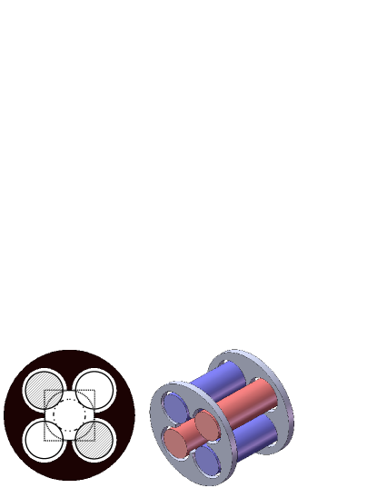
Figure 8: (Color Online) Description of the proposed alternative geometry, #4. The electric connections are the same as for trap #2, see table 1 for details. The DC electrodes geometry has been chosen so that the inner cut corresponds to the circumference inscribed in a square defined by the four rod centres.

The evolution along the $z$-axis of the averaged anharmonic contribution $\langle\zeta(z_{k})\rangle$ is shown in Fig 6. We observe that the anharmonic content is comparable to the configuration #2 up to $z_{k}/z_{0}\sim 0.4$ and lower than #1.1 for the rest of the trap.

Regarding the DC-voltages, the correlation coefficient $R^{2}$ is found to be smaller than $0.9990$ for $z_{k}/z_{0}\leq 0.28$. Although the degree of harmonicity on the axial potential is not as high as for trap #2, this alternative geometry only needs an applied voltage of 37 V in order to have $\Delta V=1$ V. For some experiments, a smaller voltage can be preferable than a perfect harmonic behaviour on the axial direction.

It is worth mentioning that the inner cut off of the DC electrodes corresponds to the circumference inscribed in a square centred on the electrodes as shown in figure 8. A geometry with the inner radius cut off equal to $r_{0}$ was also studied. The voltage required in that case for a potential depth $\Delta V=1$ V was further reduced to 3.8 V. However, this reduced shielding is paid by an increase of the anharmonicity which reaches the level of the worse geometry #1.2. This comparison shows that the anharmonic contributions are very sensitive to the position of the inner cut-off radius and configuration #4 is a good solution to reduce these contributions.

6 Conclusion

The anharmonic contribution to the potential created by a linear quadrupole trap has been studied for a large trap volume for several implementations of the DC and RF electrodes. We found that while the anharmonic content is similar at the centre of the trap in all the different implementations, they behave extremely differently further away. The already operated configurations #1.1 and #2 as well as the proposed configuration #4 achieve similar good performances for $z_{k}/z_{0}<0.5$. Furthermore, for $z_{k}/z_{0}>0.5$ the RF potential of configuration #4 keeps a level of anharmonicity intermediate between #2 and #1.1. The rather complicated electronic set-up needed for the implementation of #1.1 and the need of high static voltages for the geometry #2, make these designs not suited for all experimental situations. The alternative geometry #4, proposed in this paper, represents therefore a trade-off between complexity of the implementation and low anharmoncities, and should allow the envisaged trapping of a very large ion cloud.

7 Acknowledgements

The authors acknowledge Fernande Vedel and Laurent Hilico for valuable comments and discussions. This work is partly funded by CNES under contract n^∘ 81915/00 and by ANR under contract ANR-08-JCJC-0053-01.

References

- [1] W. Paul, Rev. Mod. Phys. 62 (1990) 531.
- [2] T. Rosenband, D. B. Hume, P. O. Schmidt, C. W. Chou, A. Brusch, L. Lorini, W. H. Oskay, R. E. Drullinger, T. M. Fortier, J. E. Stalnaker, S. A. Diddams, W. C. Swann, N. R. Newbury, W. M. Itano, D. J. Wineland, J. C. Bergquist, Frequency ratio of Al+ and Hg+ single-ion optical clocks; metrology at the 17th decimal place, science 319 (2008) 1808.
-
[3]
H. Häffner, W. Hänsel, C. F. Roos, J. Benhelm, D. Chek-Al-Kar,
M. Chwalla, T. Körber, U. D. Rapol, M. Riebe, P. O. Schmidt, C. Becher,
O. Gühne, W. Dür, R. Blatt,
Scalable multiparticle
entanglement of trapped ions, Nature 438 (7068) (2005) 643–646.
doi:10.1038/nature04279.
URL http://dx.doi.org/10.1038/nature04279 - [4] D. B. Hume, T. Rosenband, D. J. Wineland, High-fidelity adaptive qubit detection through repetitive quantum nondemolition measurements, Phys. Rev. Lett. 99 (2007) 120502.
- [5] M. Drewsen, C. Brodersen, L. Hornekær, J. S. Hangst, J. P. Schiffer, Large ion crystals in a linear Paul trap, Phys. Rev. Lett. 81 (14) (1998) 2878–2881.
- [6] R. March, J. Todd, Practical aspects of Ion Trap Spectrometry, vols. 1, 2, 3. CRC Press, New York, 1995
- [7] C. Schrama, E. Peik, W. Smith, H. Walther, Novel miniature ion traps, Optics Communications 101 (1993) 32–36.
- [8] N. McLachlan, Theory and Application of Mathieu Functions, Clarendon, Oxford, 1947.
- [9] M. Drewsen, A. Brøner, Harmonic linear Paul trap: Stability diagram and effective potentials, Phys. Rev. A 62 (2000) 045401.
- [10] H. Dehmelt, Radiofrequency spectroscopy of stored ions I: storage, Advances in Atomic and Molecular Physics 3 (1967) 53–72.
- [11] V. L. Ryjkov, X. Zhao, H. A. Schuessler, Simulations of the rf heating rates in a linear quadrupole ion trap, Phys. Rev. A 71 (3) (2005) 033414. doi:10.1103/PhysRevA.71.033414.
- [12] Y. Wang, J. Franzen, K. Wanczek, Int. J. of Mass Spectrom. and Ion Physics 124 (1993) 125–196.
- [13] R. Alheit, C. Henning, R. Morgenstern, F. Vedel, G. Werth, Observation of instabilities in a Paul trap with higher-order anharmonicities, Appl. Phys. B 61 (1995) 277–283.
- [14] M. Vedel, J. Rocher, M. Knoop, F. Vedel, Evidence of radial-axial motion couplings for an r.f. stored ion cloud, Appl. Phys. B 66 (1998) 191–196.
- [15] A. J. Reuben, G. B. Smith, P. Moses, A. V. Vagov, M. D. Woods, D. B. Gordon, R. W. Munn, Ion trajectories in exactly determined quadrupole fields, International Journal of Mass Spectrometry and Ion Processes 154 (1-2) (1996) 43 – 59.
- [16] G. Wu, R. G. Cooks, Z. Ouyang, Geometry optimization for the cylindrical ion trap: field calculations, simulations and experiments, International Journal of Mass Spectrometry 241 (2-3) (2005) 119 – 132.
- [17] H. C. Nägerl, W. Bechter, J. Eschner, F. Schmidt-Kaler, R. Blatt, Appl. Phys. B 66 (1998) 603.
- [18] http://www.simion.com.
- [19] G. Strang, G. Fix, An Analysis of the Finite Element Method, Prentice-Hall, Inc., Englewood Cliffs, N.J., 1973.
- [20] P. Bevington, Data Reduction and Error Analysis for the Physical Sciences, McGraw-Hill Book Company, New York, 1969.
- [21] L. Turner, Collective effects on equilibria of trapped charged plasmas, Physics of Fluids 30 (1987) 3196.