Bilinear approach to the quasi-periodic wave solutions of supersymmetric equations in superspace $\mathbb{R}_{\Lambda}^{2,1}$
Engui Fan
School of Mathematical Sciences and Key Laboratory of Mathematics for Nonlinear Science,
Fudan University, Shanghai, 200433, P.R. China

 
Abstract

We devise a lucid and straightforward way for explicitly constructing quasi-periodic wave solutions (also called multi-periodic wave solutions) of supersymmetric equations in superspace $\mathbb{R}_{\Lambda}^{2,1}$ over two-dimensional Grassmann algebra $G_{1}(\sigma)$. Once a nonlinear equation is written in a bilinear form, its quasi-periodic wave solutions can be directly obtained by using a formula. Moreover, properties of these solutions are investigated in detail by analyzing their structures, plots and asymptotic behaviors. The relations between the quasi-periodic wave solutions and soliton solutions are rigorously established. It is shown that the soliton solutions can be obtained only as limiting cases of the quasi-periodic wave solutions under small amplitude limits in superspace $\mathbb{R}_{\Lambda}^{2,1}$. We find that, in contrast to the purely bosonic case, there is an interesting influencing band occurred among the quasi-periodic waves under the presence of the Grassmann variable. The quasi-periodic waves are symmetric about the band but collapse along with the band. Furthermore, the amplitudes of the quasi-periodic waves increase as the waves move away from the band. The efficiency of our proposed method can be demonstrated on a class variety of supersymmetric equations such as those considered in this paper, $\mathcal{N}=1$ supersymmetric KdV, Sawada-Kotera-Ramani and Ito’s equations, as well as $\mathcal{N}=2$ supersymmetric KdV equation.
Keywords: supersymmetric equations; super-Hirota’s bilinear form; Riemann theta function; quasi-periodic wave solutions; soliton solutions.
PACS numbers: 11.30.Pb; 05.45.Yv; 02.30.Gp; 45.10.-b.
 
1. Introduction

The algebro-geometric solutions or finite gap solutions of nonlinear equations were originally obtained on the KdV equation based on inverse spectral theory and algebro-geometric method developed by pioneers such as Novikov, Dubrovin, Mckean, Lax, Its and Matveev et al. [2]-[6] in the late 1970s. In fact, such a solution is an expression written in terms of the Riemann theta functions. Hence it is also called a quasi-periodic solution due to the quasi-periodicity of the theta functions. By now this theory has been extended to a large class of nonlinear integrable equations including sine-Gordon equation, Camassa-Holm equation, Thirring model equation, Kadomtsev-Petviashvili equation, Ablowitz-Ladik lattice and Toda lattice [7]-[17].

The quasi-periodic solutions have important applications in physics. For instance, they can describe the nonlinear interaction of several modes. All the main physical characteristics of the quasi-periodic solutions (wave numbers, phase velocities, amplitudes of the interacting modes) are defined by a compact Riemann surface. There are numerous applications of the finite-gap integration theory in condensed matter physics, state physics and fluid mechanics. For example, in peierls state, phonon produce a finite-gap potential for electrons, and the peierls state is a lattice of solutions at low densities of electrons [7]. A most famous mechanical system, the Kowalewski top, was the focus of interest in the 19th century. The equation of motion of the top can be solved through finite-gap theory [7]. A problem of fundamental interest in fluid mechanics is to provide an accurate description of waves on a water surface. The Kadomtsev-Petviashvili equation is known to describe the evolution of waves in shallow water and admits a large family of quasi-periodic solutions. Each solution has $N$ independent phases. Experiments demonstrate the existence of genuinely two-dimensional shallow water waves that are full periodic in two spatial directions and time. The comparisons with experiments showed that the two-periodic wave solutions of the KP equation describe shallow water waves with much accuracy [18, 19].

The algebro-geometric theory, however, needs Lax pairs and involves complicated calculus on the Riemann surfaces. It is rather difficult to directly determine the characteristic parameters of waves such as frequencies and phase shifts for a function of given wave-numbers and amplitudes. On the other hand, the bilinear derivative method developed by Hirota is a powerful approach for constructing exact solution of nonlinear equations. Once a nonlinear equation is written in bilinear forms by a dependent variable transformation, then multi-soliton solutions are usually obtained [20]–[26]. It was based on Hirota forms that Nakamura proposed a convenient way to construct a kind of quasi-periodic solutions of nonlinear equations [27, 28, 29], where the periodic wave solutions of the KdV equation and the Boussinesq equation were obtained. Such a method indeed exhibits some advantages over algebro-gometric methods. For example, it does not need any Lax pairs and Riemann surface for the considered equation, allows the explicit construction of multi-periodic wave solutions, only relies on the existence of the Hirota’s bilinear form, as well as all parameters appearing in Riemann matrix are arbitrary. Recently, further development was made to investigate the discrete Toda lattice, (2+1)-dimensional Kadomtsev-Petviashvili equation and Bogoyavlenskii’s breaking soliton equation [30]-[35]. Indeed there are some differences between quasi-periodic solutions and algebro-geometric solutions. A quasi-periodic solution needs not be an algebro-geometric one. Sometimes a quasi-periodic solution may not correspond to any Riemann surface and is generically associated with infinite bands, not just finitely-many, for instance with a Riemann surface of infinite genus.

The concept of supersymmetry was originally introduced and developed for applications in elementary particle physics thirty years ago [36]–[38]. It is found that supersymmetry can be applied to a variety of problems such as relativistic, non-relativistic physics and nuclear physics. In recent years, supersymmetry has been a subject of considerable interest both in physics and mathematics. The mathematical formulation of the supersymmetry is based on the introduction of Grassmann variables along with the standard ones [39]. In a such way, a number of well known mathematical physical equations have been generalized into the supersymmetric analogues, such as supersymmetric versions of sine-Gordon, KdV, KP hierarchy, Boussinesq, MKdV etc. [40]–[50]. It has been shown that these supersymmetric integrable systems possess bi-Hamiltonian structure, Painleve property, infinite many symmetries, Darboux transformation, Backlund transformation, bilinear form and multi-soliton solutions. The systematic bilinear transcription of supersymmetric equations was introduced by Carstea [43, 44]. This required an extension of the Hirota’s bilinear operator to supersymmetric case. Despite this bilinearization of supersymmetric equations, the standard construction did not lead to malti-soliton solutions. In recent years, Carsta, Liu, Ghosh et al. have done much on the construction of soliton solutions of supersymmetric equations [43]–[50] . However, the quasi-periodic solutions of the supersymmetric systems, which can be considered as a generalization of the soliton solutions, are still not available (both by algebro-geometric method and by bilinear methods or others) to the knowledge of the author.

The motivation of this paper is to show how the quasi-periodic wave solutions of nonlinear supersymmetric equations can be constructed with Hirota’s bilinear method in superspace. To achieve this aim, we devise a Riemannn theta function formula, which actually provides us a lucid and straightforward way for applying in a class of nonlinear supersymmetric equations. Once a nonlinear equation is written in bilinear forms, then the quasi-periodic wave solutions of the nonlinear equation can be obtained directly by using the formula. This method considerably improves the key steps of the existing methods, where repetitive recursion and computation must be preformed for each equation [30]-[35]. As illustrative example, we shall construct quasi-periodic wave solutions to the $\mathcal{N}=1$ supersymmetric Sawada-Kotera-Ramani equation and $\mathcal{N}=2$ supersymmetric KdV equation.

The organization of this paper is as follows. In section 2, we briefly give some properties on superspace and super-Hirota bilinear operators. In section 3, we introduce a super Riemann theta function and discuss its quasi-periodicity. In particular, we provide a key formula for constructing periodic wave solutions of supersymmetric equations. As applications of our method, in section 4 and section 5, we construct one- and two-periodic wave solutions to the $\mathcal{N}=1$ supersymmetric Sawada-Kotera-Ramani equation and $\mathcal{N}=2$ supersymmetric KdV equation, respectively. The propagation of the quasi-periodic waves are displayed with help of software Mathematica. In addition, we further present a simple and effective limiting procedure to analyze asymptotic behavior of the periodic wave solutions. It is rigorously shown that the quasi-periodic wave solutions tend to the soliton solutions under small amplitude limits. At last, we briefly discuss the conditions on the construction of multi-periodic wave solutions of supersymmetric equations in section 6.
2. Super space and super-Hirota bilinear form

To fix the notations and make our presentation self-contained, we briefly recall some properties about superanalysis and super-Hirota bilinear operators. The details about superanalysis refer, for instance, to Vladimirov’s work [51, 52].

A linear space $\Lambda$ is called $Z_{2}$-graded if it represented as a direct sum of two subspaces

$$\Lambda=\Lambda_{0}\oplus\Lambda,$$

where elements of the spaces $\Lambda_{0}$ and $\Lambda_{1}$ are homogeneous. We assume that $\Lambda_{0}$ is a subspace consisting of even elements and $\Lambda_{1}$ is a subspace consisting of odd elements. For the element $f\in\Lambda$ we denote by $f_{0}$ and $f_{1}$ its even and odd components. A parity function is introduced on the $\Lambda$, namely,

$$|f|=\left\{\begin{matrix}0,\ \ {\rm if}\ \ f\in\Lambda_{0},\\ \ 1,\ \ {\rm if}\ \ f\in\Lambda_{1}.\end{matrix}\right.$$

We introduce an annihilator of the set of odd elements by setting

$${}^{\perp}\Lambda_{1}=\{\lambda\in\Lambda:\lambda\Lambda_{1}=0\}.$$

A superalgebra is a $Z_{2}$-graded space $\Lambda=\Lambda_{0}\oplus\Lambda$ in which, besides usual operations of addition and multiplication by numbers, a product of elements is defined with the usual distribution law:

$$a(\alpha b+\beta c)=\alpha ab+\beta ac,\ \ (\alpha b+\beta c)a=\alpha ba+\beta ca,$$

where $a,b,c\in\Lambda$ and $\alpha,\beta\in\mathbb{C}.$ Moreover, a structure on $\Lambda$ is introduced of an associative algebra with a unite $e$ and even multiplication i.e., the product of two even and two odd elements is an even element and the product of an even element by an odd one is an odd element: $|ab|=|a|+|b|$ mod (2).

A commutative superalgebra with unit $e=1$ is called a finite-dimensional Grassmann algebra if it contains a system of anticommuting generators $\sigma_{j},j=1,\cdots,n$ with the property: $\sigma_{j}\sigma_{k}+\sigma_{k}\sigma_{j}=0,\ j,k=1,2,\cdots,n$, in particular, $\sigma_{j}^{2}=0$. The Grassmann algebra will be denote by $G_{n}=G_{n}(\sigma_{1},\cdots,\sigma_{n})$.

The monomials $\{e_{0},e_{i}=\sigma_{j_{1}}\cdots\sigma_{j_{n}}\}$, $j=(j_{1}<\cdots<j_{n})$ form a basis in the Grassmann algebra $G_{n}$, $\dim G_{n}=2^{n}$. Then it follows that any element of $G_{n}$ is a linear combination of monomials $\sigma_{j_{1}}\cdots\sigma_{j_{k}},\ j_{1}<\cdots<j_{k}$, that is,

$$f=f_{0}+\sum_{k\geq 0}\sum_{j_{1}<\cdots<j_{k}}f_{j_{1}\cdots j_{k}}\sigma_{j_{1}}\cdots\sigma_{j_{k}},$$

where the coefficients $f_{j_{1}\cdots j_{k}}\in\mathbb{C}$.

Definition 1. Let $\Lambda=\Lambda_{0}\oplus\Lambda$ be a commutative Banach superalgebra, then the Banach space

$$\mathbb{R}_{\Lambda}^{m,n}=\Lambda_{0}^{m}\times\Lambda_{1}^{n}$$

is called a superspace of dimension $(m,n)$ over $\Lambda$. In particular, if $\Lambda_{0}=\mathbb{C}$ and $\Lambda_{1}=0$, then $\mathbb{R}_{\Lambda}^{m,n}=\mathbb{C}^{m}.$

A function $f(\boldsymbol{x}):\mathbb{R}_{\Lambda}^{m,n}\rightarrow\Lambda$ is said to be superdifferentiable at the point $x\in\mathbb{R}_{\Lambda}^{m,n}$, if there exist elements $F_{j}(\boldsymbol{x})$ in $\Lambda,\ j=1,\cdots,m+n$, such that

$$f(\boldsymbol{x}+\boldsymbol{h})=f(\boldsymbol{x})+\sum_{j=1}^{m+n}\langle F_{j}(\boldsymbol{x}),h_{j}\rangle+o(\boldsymbol{x},\boldsymbol{h}),$$

where $\boldsymbol{x}=(x_{1},\cdots,x_{m},x_{m+1},\cdots,x_{n})$ with components $x_{j},j=1,\cdots,m$ being even variable and $x_{m+j}=\theta_{j},j=1,\cdots,n$ being Grassmann odd ones. The vector $\boldsymbol{h}=(h_{1},\cdots,h_{m}$, $h_{m+1},\cdots,h_{m+n})$ with $(h_{1},\cdots,h_{m})\in\Lambda_{0}^{m}$ and $(h_{m+1},\cdots,h_{m+n})\in\Lambda_{1}^{n}$. Moreover,

$$\lim_{\parallel\boldsymbol{h}\parallel\rightarrow 0}\frac{\parallel o(\boldsymbol{x},\boldsymbol{h})\parallel}{\parallel\boldsymbol{h}\parallel}\longrightarrow 0.$$

The $F_{j}(\boldsymbol{x})$ are called the super partial derivative of $f$ with respect to $x_{j}$ at the point $\boldsymbol{x}$ and are denoted, respectively, by

$$\frac{\partial f(\boldsymbol{x})}{\partial x_{j}}=F_{j}(\boldsymbol{x}),\ j=1,\cdots,m+n.$$

The derivatives $\frac{\partial f(\boldsymbol{x})}{\partial x_{j}}$ with respect to even variables $x_{j},\ j=1,2,\cdots n$ are uniquely defined. While the derivatives $\frac{\partial f(\boldsymbol{x})}{\partial\theta_{j}}$ to odd variables $\theta_{j}=x_{j+n},\ j=1,2,\cdots m$ are not uniquely defined, but with an accuracy to within an addition constant $c\sigma_{1}\cdots\sigma_{n},c\in\mathbb{C}$ from an annihilator ${}^{\perp}G_{n}$ of finite-dimensional Grassmann algebra $G_{n}$.

The super derivative also satisfies Leibniz formula

$(2.1)$ $$\frac{\partial(f(\boldsymbol{x})g(\boldsymbol{x}))}{\partial x_{j}}=\frac{\partial f(\boldsymbol{x})}{\partial x_{j}}g(\boldsymbol{x})+(-1)^{|x_{j}||f|}f(\boldsymbol{x})\frac{\partial g(\boldsymbol{x})}{\partial x_{j}},\ j=1,\cdots,m+n.$$

Denote by $\mathcal{P}(\Lambda_{1}^{n},\Lambda)$ the set of polynomials defined on $\Lambda_{1}^{n}$ with value in $\Lambda$. We say that a super integral is a map $I:\mathcal{P}(\Lambda_{1}^{n},\Lambda)\rightarrow\Lambda$ satisfying the following condition is an super integral about Grassmann variable

(1) A linearity: $I(\mu f+\nu g)=\mu I(f)+\nu I(g),\ \mu,\nu\in\Lambda,\ f,g\in\mathcal{P}(\Lambda_{1}^{n},\Lambda);$

(2) translation invariance: $I(f_{\xi})=I(f)$, where $f_{\xi}=f(\boldsymbol{\theta}+\boldsymbol{\xi})$ for all $\boldsymbol{\xi}\in\Lambda_{1}^{n}$, $f\in\mathcal{P}(\Lambda_{1}^{n},\Lambda).$

We denote $I(\theta^{\varepsilon})=I_{\varepsilon}$, where $\varepsilon$ belongs to the set of multiindices $N_{n}=\{\boldsymbol{\epsilon}=(\varepsilon_{1},\cdots,\varepsilon_{n}),\varepsilon_{j}=0,1,\boldsymbol{\theta}^{\varepsilon}=\theta_{1}^{\varepsilon_{1}}\cdots\theta_{n}^{\varepsilon_{n}}\not\equiv 0\}$. In the case when $I_{\varepsilon}=0,\varepsilon\in N_{n},|\varepsilon|\leq n=n-1$, such kind of integral has the form

$$I(f)=J(f)I(1,\cdots,1),$$

where

$$J(f)=\frac{\partial^{n}f(0)}{\partial\theta_{1}\cdots\partial\theta_{n}}.$$

Since the derivative is defined with an accurcy to with an additive constant form the annihilator ${}^{\perp}L_{n}$, $L_{n}=\{\theta_{1}\cdots\theta_{n},\boldsymbol{\theta}\in\Lambda_{1}^{n}\}$, it follows that $J:\mathcal{P}\rightarrow\Lambda/^{\perp}L_{n}$ is single-valued mapping. This mapping also satisfies the conditions 1 and 2, and therefore we shall call it an integral and denote

$$J(f)=\int f(\boldsymbol{\theta})d\boldsymbol{\theta}=\int\theta_{1}\cdots\theta_{n}d\theta_{1}\cdots d\theta_{n},$$

which has properties:

$(2.2)$ $\displaystyle\int\theta_{1}\cdots\theta_{n}d\theta_{1}\cdots d\theta_{n}=1,$

$$\int\frac{\partial f}{\partial\theta_{j}}d\theta_{1}\cdots d\theta_{n}=0,\ j=1,\cdots,n.$$

$$\int f(\boldsymbol{\theta})\frac{\partial g(\boldsymbol{\theta})}{\partial\theta_{j}}d\boldsymbol{\theta}=(-1)^{1+|g|}\int\frac{\partial f(\boldsymbol{\theta})}{\partial\theta_{j}}g(\boldsymbol{\theta})d\boldsymbol{\theta}.$$

In this paper, we consider functions with two ordinary even variables $x,t$ and a Grassmann odd variable $\theta$. The associated space $\mathbb{R}_{\Lambda}^{2,1}=\Lambda_{0}^{2}\times\Lambda_{1}$ (we may take $\Lambda_{0}=\mathbb{R}$ or $\mathbb{C}$) is a superspace over Grassmann algebra $G_{1}(\sigma)=G_{1,0}\oplus G_{1,1}$, whose elements have the form

$$f=f_{0}+f_{1}\sigma.$$

where $e=1$ is a unit, $\sigma$ is anticommuting generator. The monomials $\{1,\sigma\}$ form a basis of the $G_{1}(\sigma)$, dim$G_{1}(\sigma)=2$. Therefore, any $\mu\in G_{1,1}$ have the form $\mu=\beta\sigma,\ \beta\in\mathbb{C}$. Under traveling wave frame in space $\mathbb{R}_{\Lambda}^{2,1}$, the phase variable should have the form

$$\xi=\alpha x+\omega t+\beta\theta\sigma.$$

For the functions $f(x,t,\theta),g(x,t,\theta):\mathbb{R}_{\Lambda}^{2,1}\rightarrow\Lambda$, the Hirota bilinear differential operators $D_{x}$ and $D_{t}$ about ordinary variables $x,t$ are defined by

$$D_{x}^{m}D_{t}^{n}f(x,t,\theta)\cdot g(x,t,\theta)=(\partial_{x}-\partial_{x^{\prime}})^{m}(\partial_{t}-\partial_{t^{\prime}})^{n}f(x,t,\theta)g(x^{\prime},t^{\prime},\theta)|_{x^{\prime}=x,t^{\prime}=t}.$$

The super-Hirota bilinear operator is defined as [43]

$$S_{x}^{N}f(x,t,\theta)\cdot g(x,t,\theta)=\sum_{j=0}^{N}(-1)^{j|f|+\frac{1}{2}j(j+1)}\left[\begin{matrix}N\\ j\end{matrix}\right]\mathfrak{D}^{N-j}f(x,t,\theta)\mathfrak{D}^{j}g(x,t,\theta),$$

where the differential operator $\mathfrak{D}=\partial_{\theta}+\theta\partial_{x}$ is the super derivative, and the super binomial coefficients are defined by

$$\left[\begin{matrix}N\\ j\end{matrix}\right]=\left\{\begin{matrix}\left(\begin{matrix}[N/2]\cr[j/2]\end{matrix}\right),{\rm if}\ \ (N,j)\not=(0,1)\ \ {\rm mod}\ \ 2,\\ \\ 0,\ \ \ \ \ \ \ {\rm otherwise}\ \ \ \ \ \ \ \ \ \ \ \ \ \ .\end{matrix}\right.$$

$[k]$ is the integer part of the real number $k$ ($[k]\leq k\leq[k]+1$).

We point out here that throughout this paper the natural number $N$ (which will denote powers, the number of phase variables, number of terms etc.) is different form $\mathcal{N}$ which is related to supersymmetry or superspace.

Proposition 1. Suppose that functions $f(x,t,\theta),g(x,t,\theta):\mathbb{R}_{\Lambda}^{2,1}\rightarrow\Lambda$, then Hirota bilinear operators $D_{x},D_{t}$ and super-Hirota bilinear operator $S_{x}$ have properties [43]

$$S_{x}^{2N}f\cdot g=D_{x}^{N}f\cdot g,$$

$$D_{x}^{m}D_{t}^{n}e^{\xi_{1}}\cdot e^{\xi_{2}}=(\alpha_{1}-\alpha_{2})^{m}(\omega_{1}-\omega_{2})^{n}e^{\xi_{1}+\xi_{2}},$$

$$S_{x}e^{\xi_{1}}\cdot e^{\xi_{2}}=[\sigma(\beta_{1}-\beta_{2})+\theta(\alpha_{1}-\alpha_{2})]e^{\xi_{1}+\xi_{2}},$$

where $\xi_{j}=\alpha_{j}x+\omega_{j}t+\beta_{j}\theta\sigma+\delta_{j}$, $\ \alpha_{j},\omega_{j},\sigma_{j},\delta_{j}\in\Lambda_{0}$ are parameters, $j=1,2$. In fact, the third formula above is defined with an accuracy to within an addition constant of the $c\sigma\in^{\perp}\Lambda_{1}$. More generally, we have

$(2.3)$ $\displaystyle F(S_{x},D_{x},D_{t})e^{\xi_{1}}\cdot e^{\xi_{2}}=F(\sigma(\beta_{1}-\beta_{2})+\theta(\alpha_{1}-\alpha_{2}),\alpha_{1}-\alpha_{2},\omega_{1}-\omega_{2})e^{\xi_{1}+\xi_{2}},$

where $F(S_{t},D_{x},D_{t})$ is a polynomial about operators $S_{t},D_{x}$ and $D_{t}$. This properties are useful in deriving Hirota’s bilinear form and constructing the quasi-periodic wave solutions of the supersymmetric equations.
3. Super Riemann theta function and addition formulae

In the following, we introduce a multi-dimensional super Riemann theta function on superspace $\mathbb{R}_{\Lambda}^{2,1}$ and discuss its quasi-periodicity, which plays a central role in the construction of quasi-periodic solutions of supersymmetric equations. The multi-dimensional Riemann theta function reads

$(3.1)$ $$\vartheta(\boldsymbol{\xi},\boldsymbol{\varepsilon},\boldsymbol{s}|\boldsymbol{\tau})=\sum_{\boldsymbol{n}\in\mathbb{{Z}}^{N}}\exp\{2\pi i\langle\boldsymbol{\xi}+\boldsymbol{\varepsilon},\boldsymbol{n}+\boldsymbol{s}\rangle-\pi\langle\boldsymbol{\tau}(\boldsymbol{n}+\boldsymbol{s}),\boldsymbol{n}+\boldsymbol{s}\rangle\}.$$

Here the integer value vector $\boldsymbol{n}=(n_{1},\cdots,n_{N})^{T}\in\mathbb{Z}^{N}$, complex parameter vectors $\boldsymbol{s}=(s_{1},\cdots,s_{N})^{T},\boldsymbol{\varepsilon}=(\varepsilon_{1},\cdots,\varepsilon_{N})^{T}\in\mathbb{{C}}^{N}$. The complex phase variables $\boldsymbol{\xi}=(\xi_{1},\cdots,\xi_{N})^{T},\ \xi_{j}=\alpha_{j}x+\omega_{j}t+\beta_{j}\theta\sigma+\delta_{j}$, $\ \alpha_{j},\omega_{j},\beta_{j},\delta_{j}\in\Lambda_{0}$, $j=1,2,\cdots,N$, where $x,t$ are ordinary variables and $\theta$ is Grassmann variable. Moreover, for two vectors $\boldsymbol{f}=(f_{1},\cdots,f_{N})^{T}$ and $\boldsymbol{g}=(g_{1},\cdots,g_{N})^{T}$, their inner product is defined by

$$\langle\boldsymbol{f},\boldsymbol{g}\rangle=f_{1}g_{1}+f_{2}g_{2}+\cdots+f_{N}g_{N}.$$

The $\boldsymbol{\tau}=(\tau_{ij})$ is a positive definite and real-valued symmetric $N\times N$ matrix, which is independent of $\theta$ and $\sigma$ in superspace $\mathbb{R}_{\Lambda}^{2,1}$. The entries $\tau_{ij}$ of the period matrix $\boldsymbol{\tau}$ can be considered as free parameters of the theta function (3.1).

In this paper, we take the $\tau$ to be pure imaginary matrix to make the theta function (3.1) real-valued. In the definition of the theta function (3.1), for the case $\boldsymbol{s}=\boldsymbol{\varepsilon}=\boldsymbol{0}$, hereafter we use $\vartheta(\boldsymbol{\xi},{\boldsymbol{\tau}})=\vartheta(\boldsymbol{\xi},\boldsymbol{0},\boldsymbol{0}|\boldsymbol{\tau})$ for simplicity. Moreover, we have $\vartheta(\boldsymbol{\xi},\boldsymbol{\varepsilon},\boldsymbol{0}|\boldsymbol{\tau})=\vartheta(\boldsymbol{\xi}+\boldsymbol{\varepsilon},\boldsymbol{\tau})$. It is obvious that the Riemann theta function (3.1) converges absolutely and superdifferentiable on superspace $\mathbb{R}_{\Lambda}^{2,1}$.

Remark 1. The period matrix $\boldsymbol{\tau}$ here is different form algebro-geometric theory discussed in [2]-[34], where it is usually constructed via a compact Riemann surface $\Gamma$ of genus $N\in\mathbb{N}$. We take two sets of regular cycle paths: $a_{1},a_{2},\cdots,a_{N}$; $b_{1},b_{2},\cdots,b_{N}$ on $\Gamma$ in such a way that the intersection numbers of cycles satisfies

$$a_{k}\circ a_{j}=b_{k}\circ b_{j}=0,a_{k}\circ b_{j}=\delta_{kj},\ \ k,j=1,\cdots,N.$$

We choose the normalized holomorphic differentials $\omega_{j},j=1,\cdots,N$ on $\Gamma$ and let

$$a_{jk}=\int_{a_{k}}{{\omega}}_{j},\ \ b_{jk}=\int_{b_{k}}{{\omega}}_{j},$$

then $N\times N$ matrices $\boldsymbol{A}=(a_{jk})$ and $\boldsymbol{B}=(b_{jk})$ are invertible. Define matrices $\boldsymbol{C}$ and $\boldsymbol{\tau}$ by

$$\boldsymbol{C}=(c_{jk})=\boldsymbol{A}^{-1},\ \ \boldsymbol{\tau}=(\tau_{jk})=\boldsymbol{A}^{-1}\boldsymbol{B}.$$

It is can be shown that the matrix $\boldsymbol{\tau}$ is symmetric and has positive definite imaginary part. However, we see that the entries in such a matrix $\boldsymbol{\tau}$ are not free and difficult to be explicitly given. $\square$

Definition 2. A function $g(\boldsymbol{x},t)$ on $\mathbb{C}^{N}\times\mathbb{C}$ is said to be quasi-periodic in $t$ with fundamental periods $T_{1},\cdots,T_{k}\in\mathbb{C}$ if $T_{1},\cdots,T_{k}$ are linearly dependent over $\mathbb{Z}$ and there exists a function $G(\boldsymbol{x},t)\in\mathbb{C}^{N}\times\mathbb{C}^{k}$ such that

$$G(\boldsymbol{x},y_{1},\cdots,y_{j}+T_{j},\cdots,y_{k})=G(\boldsymbol{x},y_{1},\cdots,y_{j},\cdots,y_{k}),\ \ {\rm for\ all}\ y_{j}\in\mathbb{C},\ j=1,\cdots,k.$$

$$G(\boldsymbol{x},t,\cdots,t,\cdots,t)=g(x,t).$$

In particular, $g(\boldsymbol{x},t)$ becomes periodic with $T$ if and only if $T_{j}=m_{j}T$. $\square$

Let’s first see the periodicity of the theta function $\vartheta(\boldsymbol{\xi},\boldsymbol{\tau})$.

Proposition 2. [53] Let $\boldsymbol{e_{j}}$ be the $j-$th column of $N\times N$ identity matrix $I_{N}$; ${\tau_{j}}$ be the $j-$th column of $\boldsymbol{\tau}$, and $\tau_{jj}$ the $(j,j)$-entry of $\boldsymbol{\tau}$. Then the theta function $\vartheta(\boldsymbol{\xi},\boldsymbol{\tau})$ has the periodic properties

$(3.2)$ $\displaystyle\vartheta(\boldsymbol{\xi}+\boldsymbol{e_{j}}+i\boldsymbol{\tau_{j}},\boldsymbol{\tau})=\exp(-2\pi i\xi_{j}+\pi\tau_{jj})\vartheta(\boldsymbol{\xi},\boldsymbol{\tau}).$

The theta function $\vartheta(\boldsymbol{\xi},\boldsymbol{\tau})$ which satisfies the condition (4.4) is called a multiplicative function. We regard the vectors $\{\boldsymbol{e_{j}},\ \ j=1,\cdots,N\}$ and $\{i\boldsymbol{\tau_{j}},\ \ j=1,\cdots,N\}$ as periods of the theta function $\vartheta(\boldsymbol{\xi},\boldsymbol{\tau})$ with multipliers $1$ and $\exp({-2\pi i\xi_{j}+\pi\tau_{jj}})$, respectively. Here, only the first $N$ vectors are actually periods of the theta function $\vartheta(\boldsymbol{\xi},\boldsymbol{\tau})$, but the last $N$ vectors are the periods of the functions $\partial^{2}_{\xi_{k},\xi_{l}}\ln\vartheta(\boldsymbol{\xi},\boldsymbol{\tau})$ and $\partial_{\xi_{k}}\ln[\vartheta(\boldsymbol{\xi}+\boldsymbol{e},\boldsymbol{\tau})/\vartheta(\boldsymbol{\xi}+\boldsymbol{h},\boldsymbol{\tau})],\ k,l=1,\cdots,N$.

Proposition 3. Let $\boldsymbol{e_{j}}$ and $\boldsymbol{\tau_{j}}$ be defined as above proposition 2. The meromorphic functions $f(\boldsymbol{\xi})$ on $\mathbb{R}_{\Lambda}^{2,1}$ are as follow

$$(i)\ \ \ \ \ f(\boldsymbol{\xi})=\partial_{\xi_{k}\xi_{l}}^{2}\ln\vartheta(\boldsymbol{\xi},\boldsymbol{\tau}),\ \ \boldsymbol{\xi}\in C^{N},\ \ \ k,l=1,\cdots,N,$$

$$(ii)\ \ \ \ f(\boldsymbol{\xi})=\partial_{\xi_{k}}\ln\frac{\vartheta(\boldsymbol{\xi}+\boldsymbol{e},\boldsymbol{\tau})}{\vartheta(\boldsymbol{\xi}+\boldsymbol{h},\boldsymbol{\tau})},\ \ \boldsymbol{\xi},\ \boldsymbol{e},\ \boldsymbol{h}\in C^{N},\ \ j=1,\cdots,N.$$

then in all two cases (i) and (ii), it holds that

$(3.3)$ $\displaystyle f(\boldsymbol{\xi}+\boldsymbol{e_{j}}+i\boldsymbol{\tau_{j}})=f(\boldsymbol{\xi}),\ \ \ \boldsymbol{\xi}\in C^{N},\ \ \ j=1,\cdots,N.$

Proof. By using (3.2), it is easy to see that

$$\frac{\vartheta^{\prime}_{\xi_{k}}(\boldsymbol{\xi}+\boldsymbol{e_{j}}+i\boldsymbol{\tau_{j}},\boldsymbol{\tau})}{\vartheta(\boldsymbol{\xi}+\boldsymbol{e_{j}}+i\boldsymbol{\tau_{j}},\boldsymbol{\tau})}=-2\pi i\delta_{jk}+\frac{\vartheta^{\prime}_{\xi_{k}}(\boldsymbol{\xi},\boldsymbol{\tau})}{\vartheta(\boldsymbol{\xi},\boldsymbol{\tau})},$$

or equivalently

$(3.4)$ $\displaystyle\partial_{\xi_{k}}\ln\vartheta(\boldsymbol{\xi}+\boldsymbol{e_{j}}+i\boldsymbol{\tau_{j}},\boldsymbol{\tau})=-2\pi i\delta_{jk}+\partial_{\xi_{k}}\ln\vartheta(\boldsymbol{\xi},\boldsymbol{\tau}).$

Differentiating (3.4) with respective to $\xi_{l}$ again immediately proves the formula (3.3) for the case (i). The formula (3.4) can be proved for the case (ii) in a similar manner. $\square$

Theorem 1. Suppose that $\vartheta(\boldsymbol{\xi},\boldsymbol{\varepsilon^{\prime}},\boldsymbol{0}|\boldsymbol{\tau})$ and $\vartheta(\boldsymbol{\xi},\boldsymbol{\varepsilon},\boldsymbol{0}|\boldsymbol{\tau})$ are two Riemann theta functions on $\mathbb{R}_{\Lambda}^{2,1}$, in which $\boldsymbol{\varepsilon}=(\varepsilon_{1},\dots,\varepsilon_{N})$, $\boldsymbol{\varepsilon^{\prime}}=(\varepsilon_{1}^{\prime},\dots,\varepsilon_{N}^{\prime})$, and $\boldsymbol{\xi}=(\xi_{1},\cdots,\xi_{N})$, $\xi_{j}=\alpha_{j}x+\omega_{j}t+\beta_{j}\theta\sigma+\delta_{j},\ \ j=1,2,\cdots,N$. Then Hirota bilinear operators $D_{x},D_{t}$ and super-Hirota bilinear operator $S_{x}$ exhibit the following perfect properties when they act on a pair of theta functions

$(3.5)$ $\displaystyle D_{x}\vartheta(\boldsymbol{\xi},\boldsymbol{\varepsilon^{\prime}},\boldsymbol{0}|\boldsymbol{\tau})\cdot\vartheta(\boldsymbol{\xi},\boldsymbol{\varepsilon},\boldsymbol{0}|\boldsymbol{\tau})$

$$=\left[\sum_{\boldsymbol{\mu}}\partial_{x}\vartheta(2\boldsymbol{\xi},\boldsymbol{\varepsilon^{\prime}}-\boldsymbol{\varepsilon},-\boldsymbol{\mu}/2|2\boldsymbol{\tau})|_{\boldsymbol{\xi}=\boldsymbol{0}}\right]\vartheta(2\boldsymbol{\xi},\boldsymbol{\varepsilon^{\prime}}+\boldsymbol{\varepsilon},\boldsymbol{\mu}/2|2\boldsymbol{\tau}),$$

$(3.6)$ $\displaystyle S_{x}\vartheta(\boldsymbol{\xi},\boldsymbol{\varepsilon^{\prime}},\boldsymbol{0}|\boldsymbol{\tau})\cdot\vartheta(\boldsymbol{\xi},\boldsymbol{\varepsilon},\boldsymbol{0}|\boldsymbol{\tau})$

$$=\left[\sum_{\boldsymbol{\mu}}\mathfrak{D}_{x}\vartheta(2\boldsymbol{\xi},\boldsymbol{\varepsilon^{\prime}}-\boldsymbol{\varepsilon},-\boldsymbol{\mu}/2|2\boldsymbol{\tau})|_{\boldsymbol{\xi}=\boldsymbol{0}}\right]\vartheta(2\boldsymbol{\xi},\boldsymbol{\varepsilon^{\prime}}+\boldsymbol{\varepsilon},\boldsymbol{\mu}/2|2\boldsymbol{\tau}),$$

where $\boldsymbol{\mu}=(\mu_{1},\cdots,\mu_{N})$, and the notation $\sum_{\boldsymbol{\mu}}$ represents $2^{N}$ different transformations corresponding to all possible combinations $\mu_{1}=0,1;\cdots;\mu_{N}=0,1$.

In general, for a polynomial operator $F(S_{x},D_{x},D_{t})$ with respect to $S_{x},D_{x}$ and $D_{t}$, we have the following useful formula

$(3.7)$ $\displaystyle F(S_{x},D_{x},D_{t})\vartheta(\boldsymbol{\xi},\boldsymbol{\varepsilon^{\prime}},\boldsymbol{0}|\boldsymbol{\tau})\cdot\vartheta(\boldsymbol{\xi},\boldsymbol{\varepsilon},\boldsymbol{0}|\boldsymbol{\tau})=\left[\sum_{\boldsymbol{\mu}}C(\boldsymbol{\varepsilon^{\prime}},\boldsymbol{\varepsilon},\boldsymbol{\mu})\right]\vartheta(2\boldsymbol{\xi},\boldsymbol{\varepsilon^{\prime}}+\boldsymbol{\varepsilon},\boldsymbol{\mu}/2|2\boldsymbol{\tau}),$

in which, explicitly

$(3.8)$ $\displaystyle C(\boldsymbol{\varepsilon},\boldsymbol{\varepsilon^{\prime}},\boldsymbol{\mu})=\sum_{\boldsymbol{n}\in\mathbb{Z}^{N}}F(\boldsymbol{\mathcal{M}})\exp\left[-2\pi\langle\boldsymbol{\tau}(\boldsymbol{n}-\boldsymbol{\mu}/2),\boldsymbol{n}-\boldsymbol{\mu}/2\rangle-2\pi i\langle\boldsymbol{n}-\boldsymbol{\mu}/2,\boldsymbol{\varepsilon^{\prime}}-\boldsymbol{\varepsilon})\right].$

where we denote $\boldsymbol{\mathcal{M}}=(4\pi i\langle\boldsymbol{n}-\boldsymbol{\mu}/2,\boldsymbol{\alpha}\rangle,\ 4\pi i\langle\boldsymbol{n}-\boldsymbol{\mu}/2,\boldsymbol{\omega}\rangle,\ 4\pi i\langle\boldsymbol{n}-\boldsymbol{\mu}/2,\boldsymbol{\sigma}+\theta\boldsymbol{\alpha}\rangle).$

Proof. For simplicity we prove the formula (3.6) for one-dimensional case. The proof for $N$-dimensional case can be performed simply by replacing one-dimensional vectors by $N$-dimensional ones.

Making use of Proposition 1, we obtain the relation

$$\Delta\equiv S_{x}\vartheta(\xi,\varepsilon^{\prime},0|{\tau})\cdot\vartheta(\xi,\varepsilon,0|{\tau})$$

$$=\sum_{m^{\prime},m\in\mathbb{Z}}\mathfrak{D}_{x}\exp\{2\pi im^{\prime}(\xi+\varepsilon^{\prime})-\pi m^{\prime 2}{\tau}\}\cdot\exp\{2\pi im(\xi+\varepsilon)-\pi m^{2}{\tau}\},$$

$$=\sum_{m^{\prime},m\in\mathbb{Z}}2\pi i(\beta\sigma+\theta\alpha)(m^{\prime}-m)\exp\left\{2\pi i(m^{\prime}+m)\xi-2\pi i(m^{\prime}\varepsilon^{\prime}+m\varepsilon)-\pi{\tau}[m^{\prime 2}+m^{2}]\right\}$$

By shifting sum index as $m=l^{\prime}-m^{\prime}$, then

$$\Delta=\sum_{l^{\prime},m^{\prime}\in\mathbb{Z}}2\pi i(\sigma+\theta\alpha)(2m^{\prime}-l^{\prime})\exp\left\{2\pi il^{\prime}\xi-2\pi i[m^{\prime}\varepsilon^{\prime}+(l^{\prime}-m^{\prime})\varepsilon]-\pi{\tau}[m^{\prime 2}+(l^{\prime}-m^{\prime})^{2}]\right\}$$

$$\stackrel{{\scriptstyle l^{\prime}=2l+\mu}}{{=}}\sum_{\mu=0,1}\ \ \sum_{l,m^{\prime}\in\mathbb{Z}}2\pi i(\beta\sigma+\theta\alpha)(2m^{\prime}-2l-\mu)\exp\{4\pi i\xi(l+\mu/2)$$

$$\ \ \ \ \ -2\pi i[m^{\prime}\varepsilon^{\prime}-(m^{\prime}-2l-\mu)\varepsilon]-\pi[m^{\prime 2}+(m^{\prime}-2l-\mu)^{2}]{\tau}\}$$

Finally letting $m^{\prime}=n+l$, we conclude that

$$\Delta=\sum_{\mu=0,1}\left[\sum_{n\in\mathbb{Z}}4\pi i(\beta\sigma+\theta\alpha)[n-\mu/2]\exp\{-2\pi i(n-\mu/2)(\varepsilon^{\prime}-\varepsilon)-2\pi{\tau}(n-\mu/2)^{2}\}\right]$$

$$\ \ \ \ \ \ \ \ \times\left[\sum_{l\in\mathbb{Z}}\exp\{2\pi i(l+\mu/2)(2\xi+\varepsilon^{\prime}+\varepsilon)-2\pi{\tau}(l+\mu/2)^{2}\right]$$

$$=\left[\sum_{\mu=0,1}\mathfrak{D}_{x}\vartheta(2\xi,\varepsilon^{\prime}-\varepsilon,-\mu/2|2{\tau})|_{\xi=0}\right]\vartheta(2\xi,\varepsilon^{\prime}+\varepsilon,\mu/2|2\tau),$$

by using the following relations

$$n+l=(n-\mu/2)+(l+\mu/2),\ \ n-l-\mu=(n-\mu/2)-(l+\mu/2).$$

In a similar way, we can prove the formula (3.5). The formula (3.7) follows from (3.5) and (3.6). $\Box$

Remark 2. The formulae (3.7) and (3.8) show that if the following equations are satisfied

$(3.9)$ $$C(\boldsymbol{\varepsilon},\boldsymbol{\varepsilon^{\prime}},\boldsymbol{\mu})=0,$$

for all possible combinations $\mu_{1}=0,1;\mu_{2}=0,1;\cdots;\mu_{N}=0,1$, in other word, all such combinations are solutions of equation (3.9), then $\vartheta(\boldsymbol{\xi},\boldsymbol{\varepsilon^{\prime}},\boldsymbol{0}|\boldsymbol{\tau})$ and $\vartheta(\boldsymbol{\xi},\boldsymbol{\varepsilon},\boldsymbol{0}|\boldsymbol{\tau})$ are $N$-periodic wave solutions of the bilinear equation

$$F(S_{t},D_{x},D_{t})\vartheta(\boldsymbol{\xi},\boldsymbol{\varepsilon^{\prime}},\boldsymbol{0}|\boldsymbol{\tau})\cdot\vartheta(\boldsymbol{\xi},\boldsymbol{\varepsilon},\boldsymbol{0}|\boldsymbol{\tau})=0.$$

We call the formula (3.9) constraint equations, whose number is $2^{N}$. This formula actually provides us an unified approach to construct multi-periodic wave solutions for supersymmetric equations. Once a supersymmetric equation is written bilinear forms, then its multi-periodic wave solutions can be directly obtained by solving system (3.9).

Theorem 2. Let $C(\boldsymbol{\varepsilon},\boldsymbol{\varepsilon^{\prime}},\boldsymbol{\mu})$ and $F(S_{x},D_{x},D_{t})$ be given in Theorem 1, and make a choice such that $\varepsilon_{j}^{\prime}-\varepsilon_{j}=\pm 1/2,\ j=1,\cdots,N$. Then

(i)  If $F(S_{x},D_{x},D_{t})$ is an even function in the form

$$F(-S_{x},-D_{x},-D_{t})=F(S_{x},D_{x},D_{t}),$$

then $C(\boldsymbol{\varepsilon},\boldsymbol{\varepsilon^{\prime}},\boldsymbol{\mu})$ vanishes automatically for the case when $\sum_{j=1}^{N}\mu_{j}$ is an odd number, namely

$(3.10)$ $$C(\boldsymbol{\varepsilon},\boldsymbol{\varepsilon^{\prime}},\boldsymbol{\mu})|_{\boldsymbol{\mu}}=0,\ \ {\rm for}\ \ \ \sum_{j=1}^{N}\mu_{j}=1,\ {\rm mod}\ 2.$$

(ii)  If $F(S_{x},D_{x},D_{t})$ is an odd function in the form

$$F(-S_{x},-D_{x},-D_{t})=-F(S_{x},D_{x},D_{t}),$$

then $C(\boldsymbol{\varepsilon},\boldsymbol{\varepsilon^{\prime}},\boldsymbol{\mu})$ vanishes automatically for the case when $\sum_{j=1}^{N}\mu_{j}$ is an even number, namely

$(3.11)$ $$C(\boldsymbol{\varepsilon},\boldsymbol{\varepsilon^{\prime}},\boldsymbol{\mu})|_{\boldsymbol{\mu}}=0,\ \ {\rm for}\ \sum_{j=1}^{N}\mu_{j}=0,\ {\rm mod}\ 2.$$

Proof. We are going to consider the case where $F(S_{x},D_{x},D_{t})$ is an even function and prove the formula (3.9). The formula (3.11) is analogous. Making transformation $\boldsymbol{n}=-\boldsymbol{\bar{n}}+\boldsymbol{\mu}\ (\boldsymbol{\bar{n}}=(\bar{n}_{1},\cdots,\bar{n}_{N}),\ \bar{n}_{j}\in\mathbb{Z},\ \ j=1,\cdots,N.$ ), and noting $F(S_{x},D_{x},D_{t})$ is even, we then deduce that

$$C(\boldsymbol{\varepsilon},\boldsymbol{\varepsilon^{\prime}},\boldsymbol{\mu})=\sum_{\boldsymbol{\bar{n}}\in\mathbb{Z}^{N}}F(-\boldsymbol{\mathcal{M}})\exp\left[-2\pi\langle\boldsymbol{\tau}(\boldsymbol{\bar{n}}-\boldsymbol{\mu}/2),\boldsymbol{\bar{n}}-\boldsymbol{\mu}/2\rangle+2\pi i\langle\boldsymbol{\bar{n}}-\boldsymbol{\mu}/2,\boldsymbol{\varepsilon^{\prime}}-\boldsymbol{\varepsilon})\right]$$

$$\ \ \ \ \ \ \ \ \ \ \ \ \ \ =C(\boldsymbol{\varepsilon},\boldsymbol{\varepsilon^{\prime}},\boldsymbol{\mu})\exp\left(4\pi i\langle\boldsymbol{\bar{n}}-\boldsymbol{\mu}/2,\boldsymbol{\varepsilon^{\prime}}-\boldsymbol{\varepsilon}\rangle\right)$$

$$\ \ \ \ \ \ \ \ \ \ \ \ \ \ =C(\boldsymbol{\varepsilon},\boldsymbol{\varepsilon^{\prime}},\boldsymbol{\mu})\exp\left(\pm 2\pi i\sum_{j=1}^{N}\bar{n}_{j}\right)\exp\left(\pm\pi i\sum_{j=1}^{N}\mu_{j}\right)$$

$$\ \ \ \ \ \ \ \ \ \ \ \ \ \ =C(\boldsymbol{\varepsilon},\boldsymbol{\varepsilon^{\prime}},\boldsymbol{\mu})\exp(\pm\pi i)=-C(\boldsymbol{\varepsilon},\boldsymbol{\varepsilon^{\prime}},\boldsymbol{\mu}),$$

which proves the formula (3.10). $\square$

Corollary 1. Let $\varepsilon_{j}^{\prime}-\varepsilon_{j}=\pm 1/2,\ j=1,\cdots,N$. Assume $F(S_{x},D_{x},D_{t})$ is a linear combination of even and odd functions

$$F(S_{x},D_{x},D_{t})=F_{1}(S_{x},D_{x},D_{t})+F_{2}(S_{x},D_{x},D_{t}),$$

where $F_{1}(S_{x},D_{x},D_{t})$ is even and $F_{2}(S_{x},D_{x},D_{t})$ is odd. In addition, $C(\boldsymbol{\varepsilon},\boldsymbol{\varepsilon^{\prime}},\boldsymbol{\mu})$ corresponding (3.8) is given by

$$C(\boldsymbol{\varepsilon},\boldsymbol{\varepsilon^{\prime}},\boldsymbol{\mu})=C_{1}(\boldsymbol{\varepsilon},\boldsymbol{\varepsilon^{\prime}},\boldsymbol{\mu})+C_{2}(\boldsymbol{\varepsilon},\boldsymbol{\varepsilon^{\prime}},\boldsymbol{\mu}),$$

where

$$C_{1}(\boldsymbol{\varepsilon},\boldsymbol{\varepsilon^{\prime}},\boldsymbol{\mu})=\sum_{\boldsymbol{n}\in\mathbb{Z}^{N}}F_{1}(\boldsymbol{\mathcal{M}})\exp\left[-2\pi\langle\boldsymbol{\tau}(\boldsymbol{n}-\boldsymbol{\mu}/2),\boldsymbol{n}-\boldsymbol{\mu}/2\rangle-2\pi i\langle\boldsymbol{n}-\boldsymbol{\mu}/2,\boldsymbol{\varepsilon^{\prime}}-\boldsymbol{\varepsilon})\right],$$

$$C_{2}(\boldsymbol{\varepsilon},\boldsymbol{\varepsilon^{\prime}},\boldsymbol{\mu})=\sum_{\boldsymbol{n}\in\mathbb{Z}^{N}}F_{2}(\boldsymbol{\mathcal{M}})\exp\left[-2\pi\langle\boldsymbol{\tau}(\boldsymbol{n}-\boldsymbol{\mu}/2),\boldsymbol{n}-\boldsymbol{\mu}/2\rangle-2\pi i\langle\boldsymbol{n}-\boldsymbol{\mu}/2,\boldsymbol{\varepsilon^{\prime}}-\boldsymbol{\varepsilon})\right].$$

Then

$(3.12)$ $\displaystyle C(\boldsymbol{\varepsilon},\boldsymbol{\varepsilon^{\prime}},\boldsymbol{\mu})=C_{2}(\boldsymbol{\varepsilon},\boldsymbol{\varepsilon^{\prime}},\boldsymbol{\mu})\ \ {\rm for}\ \ \ \sum_{j=1}^{N}\mu_{j}=1,\ {\rm mod}\ 2,$

$(3.13)$ $\displaystyle C(\boldsymbol{\varepsilon},\boldsymbol{\varepsilon^{\prime}},\boldsymbol{\mu})=C_{1}(\boldsymbol{\varepsilon},\boldsymbol{\varepsilon^{\prime}},\boldsymbol{\mu}),\ \ {\rm for}\ \sum_{j=1}^{N}\mu_{j}=0,\ {\rm mod}\ 2.$

Proof. In a similar to the proof of Theorem 2, shifting sum index as $\boldsymbol{n}=-\boldsymbol{\bar{n}}+\boldsymbol{\mu}$, and using $F_{1}(S_{x},D_{x},D_{t})$ even and $F_{2}(S_{x},D_{x},D_{t})$ odd, we have

$(3.14)$ $\displaystyle C(\boldsymbol{\varepsilon},\boldsymbol{\varepsilon^{\prime}},\boldsymbol{\mu})=C_{1}(\boldsymbol{\varepsilon},\boldsymbol{\varepsilon^{\prime}},\boldsymbol{\mu})+C_{2}(\boldsymbol{\varepsilon},\boldsymbol{\varepsilon^{\prime}},\boldsymbol{\mu})$

$$\ \ \ \ \ \ \ \ \ \ \ \ \ \ =\left[C_{1}(\boldsymbol{\varepsilon},\boldsymbol{\varepsilon^{\prime}},\boldsymbol{\mu})-C_{2}(\boldsymbol{\varepsilon},\boldsymbol{\varepsilon^{\prime}},\boldsymbol{\mu})\right]\exp\left(\pm\pi i\sum_{j=1}^{N}\mu_{j}\right).$$

Then for $\sum_{j=1}^{N}\mu_{j}=1,\ {\rm mod}\ 2$, the equation (3.15) gives

$$C_{1}(\boldsymbol{\varepsilon},\boldsymbol{\varepsilon^{\prime}},\boldsymbol{\mu})=0,$$

which implies the formula (3.12). The formula (3.13) is analogous. $\square$

The theorem 2 and corollary 1 are very useful to deal with coupled super-Hirota’s bilinear equations, which will be seen in the following section 5.

By introducing differential operators

$$\nabla=(\partial_{\xi_{1}},\partial_{\xi_{2}},\cdots,\partial_{\xi_{N}}),$$

$$\partial_{x}=\alpha_{1}\partial_{\xi_{1}}+\alpha_{2}\partial_{\xi_{2}}+\cdots+\alpha_{N}\partial_{\xi_{N}}=\boldsymbol{\alpha}\cdot\nabla,$$

$$\partial_{t}=\omega_{1}\partial_{\xi_{1}}+\omega_{2}\partial_{\xi_{2}}+\cdots+\omega_{N}\partial_{\xi_{N}}=\boldsymbol{\omega}\cdot\nabla,$$

$$\mathfrak{D}=(\sigma_{1}+\theta\alpha_{1})\partial_{\xi_{1}}+(\sigma_{2}+\theta\alpha_{2})\partial_{\xi_{2}}+\cdots+(\sigma_{N}+\theta\alpha_{N})\partial_{\xi_{N}}=(\boldsymbol{\sigma}+\theta\boldsymbol{\alpha})\cdot\nabla,$$

then we have

$(3.15)$ $\displaystyle\mathfrak{D}\partial_{x}^{k}\partial_{t}^{j}\vartheta(\boldsymbol{\xi},\boldsymbol{\tau})=[(\boldsymbol{\sigma}+\theta\boldsymbol{\alpha})\cdot\nabla](\boldsymbol{\alpha}\cdot\nabla)^{k}(\boldsymbol{\omega}\cdot\nabla)^{j}\vartheta(\boldsymbol{\xi},\boldsymbol{\tau})$

$$=(\boldsymbol{\sigma}\cdot\nabla)(\boldsymbol{\alpha}\cdot\nabla)^{k}(\boldsymbol{\omega}\cdot\nabla)^{j}\vartheta(\boldsymbol{\xi},\boldsymbol{\tau})+\theta(\boldsymbol{\alpha}\cdot\nabla)^{k+1}(\boldsymbol{\omega}\cdot\nabla)^{j}\vartheta(\boldsymbol{\xi},\boldsymbol{\tau}),$$

$$j,k=0,1,\cdots.$$

4. $\mathcal{N}=1$ supersymmetric Sawada-Kotera-Ramani equation

The supersymmetric Sawada-Kotera-Ramani equation takes the form

$(4.1)$ $\displaystyle\phi_{t}+\mathfrak{D}^{2}\left[10(\mathfrak{D}\phi)\mathfrak{D}^{4}\phi+5(\mathfrak{D}^{5}\phi)\phi+15(\mathfrak{D}\phi)^{2}\phi\right]+\mathfrak{D}^{10}\phi=0,$

where $\phi=\phi(x,t,\theta):\mathbb{R}_{\Lambda}^{2,1}\rightarrow\mathbb{R}_{\Lambda}^{0,1}$ is fermionic superfield depending on usual independent variable $x$, $t$ and Grassmann variable $\theta$. This equation was first proposed by Carstea [43]. The soliton solutions, Lax representation and infinite conserved quantities of the equation have been further obtained recently [56, 57]. Here we are interested in quasi-periodic wave solutions to the supersymmetric equation (4.1). We will show that the soliton solutions can be obtained as limiting case of these quasi-periodic solutions.

To apply the Hirota bilinear method in superspace for constructing multi-periodic wave solutions of the equation (4.1), we hope more fee variables and consider a general variable transformation

$(4.2)$ $$\phi=\phi_{0}+2\mathfrak{D}^{3}\ln f(x,t,\theta),$$

where $f(x,t,\theta):\mathbb{R}_{\Lambda}^{2,1}\rightarrow\mathbb{R}_{\Lambda}^{1,0}$ is an even superfield and $\phi_{0}=\phi_{0}(\theta):\mathbb{R}_{\Lambda}^{2,1}\rightarrow\mathbb{R}_{\Lambda}^{0,1}$ is an odd special solution of the equation (4.1). Substituting (4.2) into (4.1) and integrating with respect to $x$, we then get the following super Hirota’s bilinear form

$(4.3)$ $\displaystyle F(S_{x},D_{x},D_{t})f\cdot f=(S_{x}D_{t}+S_{x}D_{x}^{5}+15\phi_{0}^{2}D_{x}^{2}+5\phi_{0}D_{x}^{4}+c)f\cdot f=0,$

where $c=c(\theta,t):\mathbb{R}_{\Lambda}^{2,1}\rightarrow\mathbb{R}_{\Lambda}^{0,1}$ is an odd integration constant. In the special case when $\phi_{0}=c=0$, starting from the bilinear equation (4.3), it is easy to find that the equation (4.1) admits one-soliton solution (also called one-supersoliton solution) in superspace $\mathbb{R}_{\Lambda}^{2,1}$ over two-dimensional Grassmann algebra $G_{1}(\sigma)$

$(4.4)$ $$\phi_{1}=2\mathfrak{D}^{3}\ln(1+e^{\eta}),$$

with phase variable $\eta=px-p^{5}t+q\theta\sigma+r$ with $p,q,r\in\Lambda_{0}$. While two-soliton solution (super two-soliton solution) reads

$(4.5)$ $$\phi_{2}=2\mathfrak{D}^{3}\ln(1+e^{\eta_{1}}+e^{\eta_{2}}+e^{\eta_{1}+\eta_{2}+A_{12}}),$$

with $\eta_{j}=p_{j}x-p_{j}^{3}t+q_{j}\theta\sigma+r_{j},\ \ j=1,2$ and

$$e^{A_{12}}=\frac{(p_{1}-p_{2})^{2}(p_{1}^{2}-p_{1}p_{2}+p_{2}^{2})}{(p_{1}+p_{2})^{2}(p_{1}^{2}+p_{1}p_{2}+p_{2}^{2})}\left(1+2\theta\sigma\frac{p_{1}q_{2}-p_{2}q_{1}}{p_{1}-p_{2}}\right),$$

and here $p_{j},q_{j},r_{j}\in\Lambda_{0},j=1,2$ are free constants.

Next, we turn to see the periodicity of the solution (4.2), the function $f$ is chosen to be a Riemann theta function, namely,

$$f(x,t,\theta)=\vartheta(\boldsymbol{\xi},\boldsymbol{\tau}),$$

where phase variable $\xi$ is taken as the form $\boldsymbol{\xi}=(\xi_{1},\cdots,\xi_{N})^{T}$, $\xi_{j}=\alpha_{j}x+\omega_{j}t+\beta_{j}\theta\sigma+\delta_{j},\ \ j=1,2,\cdots,N.$ With Proposition 3, we refer to

$$\phi=\phi_{0}+2\sum_{k,l=1}^{N}\alpha_{k}(\beta_{l}\sigma+\theta\alpha_{l})\partial_{\xi_{k}\xi_{l}}^{2}\ln\vartheta(\boldsymbol{\xi},\boldsymbol{\tau}),$$

which shows that the solution $\phi$ is indeed a quasi-periodic function with $2N$ fundamental periods $\{\boldsymbol{e_{j}},\ \ j=1,\cdots,N\}$ and $\{i\boldsymbol{\tau}_{j},\ \ j=1,\cdots,N\}$. The quasi-periodic means that $\phi$ is periodic in each of the $N$ phases $\{\xi_{j},\ \ j=1,\cdots,N\}$, if the other $N-1$ phases are fixed.
3.1. One-periodic waves and asymptotic analysis

We first consider one-periodic wave solutions of the equation (4.1). As a simple case of the theta function (3.1) when $N=1,s=\varepsilon=0$, we take $f$ as

$(4.6)$ $$f(x,t,\theta)=\vartheta(\xi,\tau)=\sum_{n\in\mathbb{Z}}\exp({2\pi in\xi-\pi n^{2}\tau}),$$

where the phase variable $\xi=\alpha x+\omega t+\beta\theta\sigma+\delta$, and the parameter $\tau>0$.

Next, we let the Riemann theta function (4.6) be a solution of the bilinear equation (4.3). By using Theorem 1 and the formula (3.9), the following two equations ( corresponding to $\mu=0$ and $1$ respectively) should be satisfied

$(4.7)$ $\displaystyle\sum_{n\in\mathbb{Z}}\{-(4\pi(n-\mu/2))^{2}(\beta\sigma+\theta\alpha)\omega-(4\pi(n-\mu/2))^{6}(\beta\sigma+\theta\alpha)\alpha^{5}-15(4\pi(n-\mu/2))^{2}\alpha^{2}\phi_{0}^{2}$

$$+5(4\pi(n-\mu/2))^{4}\alpha^{4}\phi_{0}+c\}\exp(-2\pi\tau(n-\mu/2)^{2})=0,\ \ \mu=0,1.$$

We introduce the notations by

$$\begin{aligned} &\lambda=e^{-\pi\tau/2},\quad\vartheta_{1}(\xi,\lambda)=\vartheta(2\mathbf{\xi},0,0|2\tau)=\sum_{n\in\mathbb{Z}}\lambda^{4n^{2}}\exp(4i\pi n\xi),\\ &\vartheta_{2}(\xi,\lambda)=\vartheta(2\xi,0,-1/2|2\tau)=\sum_{n\in\mathbb{Z}}\lambda^{(2n-1)^{2}}\exp[2i\pi(2n-1)\xi],\end{aligned})$$

the equation (4.7) can be written as a linear system about $\omega,c$

$(4.8)$ $\displaystyle(\beta\sigma+\theta\alpha)\vartheta_{j}^{\prime\prime}\omega+(\beta\sigma+\theta\alpha)\alpha^{5}\vartheta_{j}^{(6)}+3\alpha^{2}\vartheta_{j}^{\prime\prime}\phi_{0}^{2}+5\alpha^{4}\vartheta_{j}^{(4)}\phi_{0}+\vartheta_{j}c=0,\ \ j=1,\ 2,$

where $\omega\in\Lambda_{0}$ is even and $c,\phi_{0}\in\Lambda_{1}$ are odd, and we have denoted the derivative value of $\vartheta_{j}(\xi,\lambda)$ at $\xi=0$ by simple notations

$$\vartheta_{j}^{\prime}=\vartheta_{j}^{\prime}(0,\lambda)=\frac{d\vartheta_{j}(\xi,\lambda)}{d\xi}|_{\xi=0},\ \ j=1,2.$$

Moreover, we see that the functions $\vartheta_{j}$ and their derivatives are independent of Grassmann variable $\theta$ and anticommuting number $\sigma$.

We take $\phi_{0}=0$ for the simplicity. It is obvious that the coefficient determinant of the system (4.8) is nonzero and $(\alpha^{5}\vartheta_{1}^{(6)},\alpha^{5}\vartheta_{2}^{(6)})^{T}\not=0$, therefore the system (4.8) admits a solution

$(4.9)$ $\displaystyle\omega=\frac{\alpha^{5}(\vartheta_{2}^{(6)}\vartheta_{1}-\vartheta_{1}^{(6)}\vartheta_{2})}{\vartheta_{1}^{\prime\prime}\vartheta_{2}-\vartheta_{2}^{\prime\prime}\vartheta_{1}},\ \ \ b_{1}=\frac{\alpha^{5}(\beta\sigma+\theta\alpha)(\vartheta_{2}^{(6)}\vartheta_{1}^{\prime\prime}-\vartheta_{1}^{(6)}\vartheta_{2}^{\prime\prime})}{\vartheta_{1}^{\prime\prime}\vartheta_{2}-\vartheta_{2}^{\prime\prime}\vartheta_{1}},$

where $\omega$ is independent of Grassmann variable $\theta$ and auticommuting number $\sigma$, and parameter $\alpha$ is free.

In this way, a one-periodic wave solution of the equation (4.1) is explicitly obtained by

$(4.10)$ $$\phi=2\mathfrak{D}^{3}\ln\vartheta(\xi,\tau),$$

with the theta function $\vartheta(\xi,\tau)$ given by (4.6) and parameters $\omega$, $c$ by (4.9), while other parameters $\alpha,\beta,\tau,\delta\in\Lambda_{0}$ are free. Among them, the three parameters $\alpha$ and $\tau$ completely dominate a one-periodic wave.

In summary, one-periodic wave (4.10) possesses the following features:

(i) It is one-dimensional, i.e. there is a single phase variable $\xi$. Moreover, it has two fundamental periods $1$ and $i\tau$ in phase variable $\xi$, but it need not to be periodic in $x$, $t$ and $\theta$ directions.

(ii) It can be viewed as a parallel superposition of overlapping one-soliton waves, placed one period apart ( see $(a)$ and $(b)$ in Figure 1 ).

(iii) Different form the purely bosonic case, it is observed shows that there is an influencing band among the one-periodic waves under the presence of the Grassmann variable (in contour plot, the bright hexagons are crests and the dark hexagons are troughs). The one-periodic waves are symmetric about the band but collapse along with the band. Furthermore, the amplitudes of the quasi-periodic waves increase as the waves move away from the band ( see $(a)$ and $(b)$ in Figure 1 ).

(iv) The quasi-periodic wave will degenerate to pure bosonic quasi-periodic wave when $\theta$ becomes small ( see Figure 2 ).

$(b)\ \ \ \ \ \ \ \ \ \ \ \ \ \ \ \ \ \ \ \ \ \ \ \ \ \ \ \ \$                   $(b)$                              
             

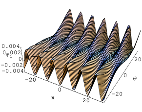
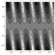
Figure 1. A one-periodic wave for $\mathcal{N}=1$ supersymmetric Sawada-Kotera-Ramani equation with parameters: $\alpha=0.1,$ $\tau=32,\sigma=0.013$. (a) Perspective view of wave. (b) Overhead view of wave, with contour plot shown.

$(b)\ \ \ \ \ \ \ \ \ \ \ \ \ \ \ \ \ \ \ \ \ \ \ \ \ \ \ \ \$                   $(b)$                              
             

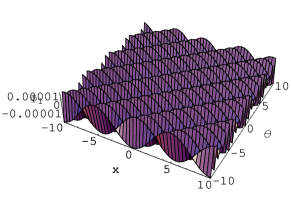
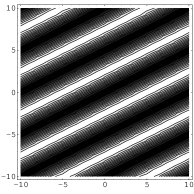
Figure 2. A purely bosonic case of one-periodic wave to $\mathcal{N}=1$ supersymmetric Sawada-Kotera-Ramani equation with parameters: $\alpha=0.1,$  $\tau=32,\ \sigma=0.013,\ \theta=0.00000001$. (a) Perspective view of wave. (b) Overhead view of wave, with contour plot shown.

In the following, we further consider asymptotic properties of the one-periodic wave solution. Interestingly, the relation between the one-periodic wave solution (4.10) and the one-soliton solution (4.4) can be established as follows.

Theorem 3. Suppose that $\omega$ and $c$ are given by (4.9), and for the one-periodic wave solution (4.10), we let

$(4.11)$ $$\alpha=\frac{p}{2\pi i},\ \ \beta=\frac{q}{2\pi i},\ \ \delta=\frac{r+\pi\tau}{2\pi i},$$

where the $p,q$ and $r$ are given in (4.4). Then we have the following asymptotic properties

$$c\longrightarrow 0,\ \ 2\pi i\xi-\pi\tau\longrightarrow\eta=px-p^{5}t+q\theta\sigma+r,$$

$$\vartheta(\xi,\tau)\longrightarrow 1+e^{\eta},\ \ {\rm as}\ \ \lambda\rightarrow 0.$$

In other words, the one-periodic solution (4.10) tends to the soliton solution (4.4) under a small amplitude limit, that is,

$(4.12)$ $$\phi\longrightarrow\phi_{1},\ \ {\rm as}\ \ \lambda\rightarrow 0.$$

Proof. Here we will directly use the system (4.8) to analyze asymptotic properties of one-periodic solution (4.10), which is more simple and effective than our original method by solving the system [30]-[34]. Since the coefficients of system (4.8) are power series about $\lambda$, its solution $(\omega,c)$ also should be a series about $\lambda$. We explicitly expand the coefficients of system (4.8) as follows

$(4.13)$ $\displaystyle\vartheta_{1}=1+2\lambda^{4}+\cdots,\quad\ \vartheta_{1}^{\prime\prime}=-32\pi^{2}\lambda^{4}+\cdots,$

$$\vartheta_{1}^{(6)}=-8192\pi^{6}\lambda^{4}+\cdots,\ \ \vartheta_{2}=2\lambda+2\lambda^{9}+\cdots$$

$$\vartheta_{2}^{\prime\prime}=-8\pi^{2}\lambda+\cdots,\ \ \ \vartheta_{1}^{(6)}=-128\pi^{6}\lambda+\cdots.$$

Let the solution of the system (4.8) be of the form

$(4.14)$ $\displaystyle\omega=\omega_{0}+\omega_{1}\lambda+\omega_{2}\lambda^{2}+\cdots=\omega_{0}+o(\lambda),$

$$c=c_{0}+c_{1}\lambda+c_{2}\lambda^{2}+\cdots=c_{0}+o(\lambda).$$

Substituting the expansions (4.13) and (4.14) into the system (4.8) (the second equation is divided by $\lambda$ ) and letting $\lambda\longrightarrow 0$, we immediately obtain the following relations

$$c_{0}=0,\ \ -8\pi^{2}(\beta\sigma+\theta\alpha)\omega_{0}+2c_{0}-128\pi^{6}(\beta\sigma+\theta\alpha)\alpha^{5}=0,$$

which has a solution

$(4.15)$ $$c_{0}=0,\ \ w_{0}=-16\pi^{4}\alpha^{5}.$$

Combining (4.14) and (4.15) then yields

$$c\longrightarrow 0,\ \ 2\pi i\omega\longrightarrow-32i\pi^{5}\alpha^{5}=-p^{5},\ \ {\rm as}\ \ \lambda\rightarrow 0.$$

Hence we conclude

$(4.16)$ $\displaystyle\hat{\xi}=2\pi i\xi-\pi\tau=px+2\pi i\omega t+q\theta\sigma+r$

$$\quad\longrightarrow px-p^{5}t+q\theta\sigma+r=\eta,\ \ {\rm as}\ \ \lambda\rightarrow 0.$$

It remains to consider asymptotic properties of the one-periodic wave solution (4.10) under the limit $\lambda\rightarrow 0$. By expanding the Riemann theta function $\vartheta(\xi,\tau)$ and by using (4.16), it follows that

$$\vartheta(\xi,\tau)=1+\lambda^{2}(e^{2\pi i\xi}+e^{-2\pi i\xi})+\lambda^{8}(e^{4\pi i\xi}+e^{-4\pi i\xi})+\cdots$$

$$\ \ \ \ \ =1+e^{\hat{\xi}}+\lambda^{4}(e^{-\hat{\xi}}+e^{2\hat{\xi}})+\lambda^{12}(e^{-2\hat{\xi}}+e^{3\hat{\xi}})+\cdots$$

$$\ \ \ \ \ \quad\longrightarrow 1+e^{\hat{\xi}}\longrightarrow 1+e^{\eta},\ \ {\rm as}\ \ \lambda\rightarrow 0,$$

which together with (4.10) lead to (4.12). Therefore we conclude that the one-periodic solution (4.10) just goes to the one-soliton solution (4.4) as the amplitude $\lambda\rightarrow 0$. $\square$
3.2. Two-periodic wave solutions and asymptotic analysis

We proceed to the construction of the two-periodic wave solutions to the supersymmetric Sawada-Kotera-Ramani equation (4.1), which are a two-dimensional generalization of one-periodic wave solutions. The two-periodic waves of interest here have three-dimensional velocity fields and two-dimensional surface patterns.

For the case when $N=2,\boldsymbol{s}=\boldsymbol{\varepsilon}=\boldsymbol{0}$ in the Riemann theta function (3.1), we takes $f$ as

$(4.17)$ $$f=\vartheta(\boldsymbol{\xi},\boldsymbol{\tau})=\sum_{\boldsymbol{n}\in\mathbb{Z}^{2}}\exp\{2\pi i\langle\boldsymbol{\xi},\boldsymbol{n}\rangle-\pi\langle\boldsymbol{\tau}\boldsymbol{n},\boldsymbol{n}\rangle\},$$

where $\boldsymbol{n}=(n_{1},n_{2})^{T}\in\mathbb{Z}^{2},\ \ \boldsymbol{\xi}=(\xi_{1},\xi_{2})^{T}\in\mathbb{C}^{2},\ \ \xi_{i}=\alpha_{j}x+\omega_{j}t+\beta_{j}\theta\sigma+\delta_{j},\ \ j=1,2$; The matrix $\boldsymbol{\tau}$ is a positive definite and real-valued symmetric ${2\times 2}$ matrix, which can takes of the form

$$\boldsymbol{\tau}=(\tau_{ij})_{2\times 2},\ \ \tau_{12}=\tau_{21},\ \ \tau_{11}>0,\ \ \tau_{22}>0,\ \ \tau_{11}\tau_{22}-\tau_{12}^{2}>0.$$

Next, we explore the conditions to make the Riemann theta function (4.17) satisfy the bilinear equation (4.3). Theorem 1 and the formula (3.9) give rise to the following four constraint equations

$(4.18)$ $\displaystyle\sum_{n_{1},n_{2}\in\mathbb{Z}}\left[-4\pi^{2}\langle 2\boldsymbol{n}-\boldsymbol{\mu},\boldsymbol{\sigma}+\theta\boldsymbol{\alpha}\rangle\langle 2\boldsymbol{n}-\boldsymbol{\mu},\boldsymbol{\omega}\rangle-64\pi^{6}\langle 2\boldsymbol{n}-\boldsymbol{\mu},\boldsymbol{\alpha}\rangle^{5}\langle 2\boldsymbol{n}-\boldsymbol{\mu},\boldsymbol{\sigma}+\theta\boldsymbol{\alpha}\rangle\right.$

$$-60\pi^{2}\langle 2\boldsymbol{n}-\boldsymbol{\mu},\boldsymbol{\alpha}\rangle^{2}\phi_{0}^{2}+80\pi^{4}\langle 2\boldsymbol{n}-\boldsymbol{\mu},\boldsymbol{\alpha}\rangle^{4}\phi_{0}+c]\exp\{-2\pi\langle\boldsymbol{\tau}(\boldsymbol{n}-\boldsymbol{\mu}/2),\boldsymbol{n}-\boldsymbol{\mu}/2\rangle\}=0,$$

where $\boldsymbol{\mu}=(\mu_{1},\mu_{2})$ takes all possible combinations of $\mu_{1},\mu_{2}=0,1$.

By introducing the notations

$$\lambda_{kl}=e^{-\pi\tau_{kl}/2},k,l=1,2,\boldsymbol{\lambda}=(\lambda_{11},\lambda_{12},\lambda_{22})$$

$$\vartheta_{j}(\boldsymbol{\xi},\boldsymbol{\lambda})=\vartheta(2\xi,\boldsymbol{0},-\boldsymbol{s}_{j}/2|2\tau)=\sum_{n_{1},n_{2}\in Z}\exp\{4\pi i\langle\boldsymbol{\xi},\boldsymbol{n}-\boldsymbol{s_{j}}/2\rangle\}\prod_{k,l=1}^{2}\lambda_{kl}^{(2n_{k}-s_{j,k})(2n_{j}-s_{j,l})},$$

$$\boldsymbol{s_{j}}=(s_{j,1},s_{j,2}),\quad j=1,2,3,4,\ \ \boldsymbol{s_{1}}=(0,0),\ \ \boldsymbol{s_{2}}=(1,0),\ \ \boldsymbol{s_{3}}=(0,1),\ \ \boldsymbol{s_{4}}=(1,1),$$

then by using (3.15), the system (4.18) can be written as a linear system

$(4.19)$ $\displaystyle[(\boldsymbol{\beta}\sigma+\theta\boldsymbol{\alpha})\cdot\nabla](\boldsymbol{\omega}\cdot\nabla)\vartheta_{j}(0,\boldsymbol{\lambda})+[(\boldsymbol{\beta}\sigma+\theta\boldsymbol{\alpha})\cdot\nabla](\boldsymbol{\alpha}\cdot\nabla)^{5}\vartheta_{j}(0,\boldsymbol{\lambda})$

$$+15(\boldsymbol{\alpha}\cdot\nabla)^{2}\vartheta_{j}(0,\boldsymbol{\lambda})\phi_{0}^{2}+5(\boldsymbol{\alpha}\cdot\nabla)^{4}\vartheta_{j}(0,\boldsymbol{\lambda})\phi_{0}+\vartheta_{j}(0,\boldsymbol{\lambda})c=0.$$

This system is easy to be solved in such a way: $\phi_{0}$ by solving a quadratic equation with one unknown; $\omega_{1},\omega_{2}$ and $c$ by solving a linear system. With such a solution $(\omega_{1},\omega_{2},\phi_{0},c)$, we then get an exact two-periodic wave solution

$(4.20)$ $$\phi=\phi_{0}+2\mathfrak{D}^{3}\ln\vartheta(\boldsymbol{\xi},\boldsymbol{\tau}),$$

with $\vartheta(\boldsymbol{\xi},\boldsymbol{\tau})$ and $\omega_{1},\omega_{2},\phi_{0},c$ given by (4.17) and (4.19), respectively, while other parameters $\beta_{1},\beta_{2},\alpha_{1},$ $\alpha_{2},\tau_{11},\tau_{22},\tau_{12},\delta_{1},\delta_{2}\in\Lambda_{0}$ are free.

In summary, two-periodic wave (4.20), which is a direct generalization of one-periodic wave, has the following features:

(i) The two-periodic wave solution is genuinely two-dimensional. Its surface pattern is two-dimensional, namely, there are two phase variables $\xi_{1}$ and $\xi_{2}$.

(ii) It has two independent spatial periods in two independent horizontal directions. It has $4$ fundamental periods $\{e_{1},e_{2}\}$ and $\{i\tau_{1},i\tau_{2}\}$ in $(\xi_{1},\xi_{2})$. It is spatially periodic in two directions $\xi_{1},\xi_{2}$, but it does not need periodic in the all $x$-, $t$- and $\theta$-directions.

(iii) As in the case of on-periodic waves, there is an influencing band among the two-periodic waves under the presence of the Grassmann variable. ( see Figure 3 ).

$(a)\ \ \ \ \ \ \ \ \ \ \ \ \ \ \ \ \ \ \ \ \ \ \ \ \ \ \ \ \$                   $(b)$                              
             

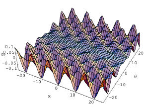
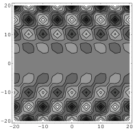
Figure 3. A two-super periodic wave for $\mathcal{N}=1$ supersymmetric Sawada-Kotera-Ramani equation with parameters: $\alpha_{1}=0.1,\alpha_{2}=-0.1,$ $\tau_{11}=2,\tau_{12}=0.2,\tau_{22}=2,\sigma_{1}=0.1,\sigma_{2}=0.1$. (a) Perspective view of wave. (b) Overhead view of wave, with contour plot shown.

At last, we consider the asymptotic properties of the two-periodic solution (4.20). In a similar way to Theorem 3, we can establish the relation between the two-periodic solution (4.20) and the two-soliton solution as follows.

Theorem 4. Assume that $(\omega_{1},\omega_{2},\phi_{0},c)^{T}$ is a solution of the system (4.19). We choose the parameters in the two-periodic wave solution (4.20) as follows

$(4.21)$ $\displaystyle\alpha_{j}=\frac{p_{j}}{2\pi i},\ \ \beta_{j}=\frac{q_{j}}{2\pi i},\ \ \delta_{j}=\frac{r_{j}+\pi\tau_{jj}}{2\pi i},\ \ \tau_{12}=-\frac{A_{12}}{2\pi},\ \ j=1,2,$

with the $p_{j},q_{j},r_{j},j=1,2$ as those given in (4.5). Then under constraint $\alpha_{1}\beta_{2}=\alpha_{2}\beta_{1}$, we have the following asymptotic relations

$(4.22)$ $\displaystyle\phi_{0}\longrightarrow 0,\ \ \ c\longrightarrow 0,\ \ 2\pi i\xi_{j}-\pi\tau_{jj}\longrightarrow p_{j}x-p_{j}^{5}t+q_{j}\theta\sigma+r_{j}=\eta_{j},\ \ j=1,2,$

$$\vartheta(\boldsymbol{\xi},\boldsymbol{\tau})\longrightarrow 1+e^{\eta_{1}}+e^{\eta_{2}}+e^{\eta_{1}+\eta_{2}+A_{12}},\ \ \ {\rm as}\ \ \lambda_{11},\lambda_{22}\rightarrow 0.$$

So the two-periodic wave solution (5.20) tends to the two-soliton solution (4.5), namely,

$$\phi\longrightarrow\phi_{2},\ \ {\rm as}\ \ \lambda_{11},\lambda_{22}\rightarrow 0.$$

Proof. From (4.21), the constraint $\alpha_{1}\beta_{2}=\alpha_{2}\beta_{1}$ leads to $p_{1}q_{2}-p_{2}q_{1}=0$, which implies that $\tau_{12}=-A_{12}/2\pi$ is independent of Grassmann variable $\theta$ according to (4.5).

In the same way as the proof of Theorem 3, we expand the Riemann function $\vartheta(\xi_{1},\xi_{2},\boldsymbol{\tau})$ in the following form

$$\vartheta(\boldsymbol{\xi},\boldsymbol{\tau})=1+(e^{2\pi i\xi_{1}}+e^{-2\pi i\xi_{1}})e^{-\pi{\tau}_{11}}+(e^{2\pi i\xi_{2}}+e^{-2\pi i\xi_{2}})e^{-\pi\tau_{22}}$$

$$\ \ \ \ \ \ \ \ \ \ \ \ +(e^{2\pi i(\xi_{1}+\xi_{2})}+e^{-2\pi i(\xi_{1}+\xi_{2})})e^{-\pi(\tau_{11}+2\tau_{12}+\tau_{22})}+\cdots$$

Further by using (4.21) and making a transformation $\hat{\omega}_{j}=2\pi i\omega_{j},j=1,2$, we get

$$\vartheta(\boldsymbol{\xi},\boldsymbol{\tau})=1+e^{\hat{\xi}_{1}}+e^{\hat{\xi}_{2}}+e^{\hat{\xi}_{1}+\hat{\xi}_{2}-2\pi\tau_{12}}+\lambda_{11}^{4}e^{-\hat{\xi}_{1}}+\lambda_{22}^{4}e^{-\hat{\xi}_{2}}+\lambda_{11}^{4}\lambda_{22}^{4}e^{-\hat{\xi}_{1}-\hat{\xi}_{2}-2\pi\tau_{12}}+\cdots$$

$$\ \ \ \ \ \longrightarrow 1+e^{\hat{\xi}_{1}}+e^{\hat{\xi}_{2}}+e^{\hat{\xi}_{1}+\hat{\xi}_{2}+A_{12}},\ \ {\rm as}\ \ \lambda_{11},\lambda_{22}\rightarrow 0,$$

where $\hat{\xi}_{j}=p_{j}x+\hat{\omega}_{j}t+p_{j}\theta\sigma+r_{j},\ \ j=1,2.$

It remains to prove that

$(4.23)$ $\displaystyle c\longrightarrow 0,\ \ \ \hat{\omega}_{j}\longrightarrow-p_{j}^{5},\ \ \hat{\xi}_{j}\longrightarrow\eta_{j},\ \ j=1,2,\ \ \ {\rm as}\ \ \lambda_{11},\lambda_{22}\rightarrow 0.$

As in the case when $N=1$, we let the solution of the system (4.19) be the form

$(4.24)$ $\displaystyle\omega_{1}=\omega_{1,0}+\omega_{1,1}\lambda_{11}+\omega_{1,2}\lambda_{22}+\cdots=\omega_{1,0}+o(\lambda_{11},\lambda_{22}),$

$$\omega_{2}=\omega_{2,0}+\omega_{2,1}\lambda_{11}+\omega_{2,2}\lambda_{22}+\cdots=\omega_{2,0}+o(\lambda_{11},\lambda_{22}),$$

$$\phi_{0}=\phi_{0,0}+\phi_{0,1}\lambda_{11}+\phi_{0,2}\lambda_{22}+\cdots=\phi_{0,0}+o(\lambda_{11},\lambda_{22}),$$

$$c=c_{0}+c_{1}\lambda_{11}+c_{2}\lambda_{22}+\cdots=c_{0}+o(\lambda_{11},\lambda_{22}).$$

Expanding functions $\vartheta_{j},j=1,2,3,4$ in the system (4.19), together with substitution of assumption (4.24), the second and third equation is divided by $\lambda_{11}$ and $\lambda_{22}$, respectively; the fourth equation is divided by $\lambda_{11}\lambda_{22}$, and letting $\lambda_{11},\lambda_{22}\longrightarrow 0$ , we then obtain

$$c_{0}=0,\ -8\pi(\beta_{1}\sigma+\theta\alpha_{1})\omega_{1}-128\pi^{6}\alpha_{1}^{5}(\beta_{1}\sigma+\theta\alpha_{1})-120\pi\alpha_{1}^{2}\phi_{0,0}^{2}+2\phi_{0,0}=0,$$

$$-8\pi(\beta_{2}\sigma+\theta\alpha_{2})\omega_{2}-128\pi^{6}\alpha_{2}^{5}(\beta_{2}\sigma+\theta\alpha_{2})-120\pi\alpha_{2}^{2}\phi_{0,0}^{2}+2\phi_{0,0}=0,$$

which has solution

$(4.25)$ $\displaystyle c_{0}=0,\ \ \phi_{0,0}=0,\ \ \ \omega_{1,0}=-16\pi^{4}\alpha_{1}^{5},\ \ \omega_{2,0}=-16\pi^{4}\alpha_{2}^{5}.$

The expressions (4.24) and (4.25) implies that

$$\phi_{0}=o(\lambda_{11},\lambda_{22})\longrightarrow 0,\ \ c=o(\lambda_{11},\lambda_{22})\longrightarrow 0,\ \ \omega_{1}=-16\pi^{4}\alpha_{1}^{5}+o(\lambda_{11},\lambda_{22})\longrightarrow-16\pi^{4}\alpha_{1}^{5},$$

$$\omega_{2}=-16\pi^{4}\alpha_{2}^{5}+o(\lambda_{11},\lambda_{22})\longrightarrow-16\pi^{4}\alpha_{2}^{5},\ \ \ {\rm as}\ \ \lambda_{11},\lambda_{22}\rightarrow 0,$$

thus proving (4.23). We conclude that the two-periodic wave solution (4.20) tends to the two-soliton solution (4.5) as $\lambda_{11},\lambda_{22}\rightarrow 0$. $\square$
4. $\mathcal{N}=2$ supersymmetric KdV equation

We consider $\mathcal{N}=2$ supersymmetric KdV equation

$(5.1)$ $\displaystyle\phi_{t}=-\phi_{xxx}+3(\phi\mathfrak{D}_{1}\mathfrak{D}_{2}\phi)_{x}+\frac{1}{2}(a-1)(\mathfrak{D}_{1}\mathfrak{D}_{2}\phi^{2})_{x}+3a\phi^{2}\phi_{x}^{2},$

which was originally introduced by Laberge and Mathieu [58, 59]. In the equation (5.1), $\phi=\phi(x,t,\theta_{1},\theta_{2}):\mathbb{R}_{\Lambda}^{2,2}\rightarrow\mathbb{R}_{\Lambda}^{0,1}$ is a superboson function depending on temporal variable $t$, spatial variable $x$ and its fermionic counterparts $\theta_{1},\theta_{2}$. The operators $\mathfrak{D}_{1}$ and $\mathfrak{D}_{2}$ are the super derivatives defined by $\mathfrak{D}_{1}=\partial_{\theta_{1}}+\theta_{1}\partial_{x},\ \ \mathfrak{D}_{2}=\partial_{\theta_{2}}+\theta_{2}\partial_{x}$ and $a$ is a parameter. The equation (5.1) is called supersymmetric KdV_a equation [60]. For the cases when $a=1$ and $a=4$, the Lax representation, Hamiltonian structure, Painleve analysis and soliton solutions of the equation (5.1) can refer to, for instance, papers [58]–[60].

Here we are interested in quasi-periodic wave solutions to the supersymmetric equation (5.1) by using Theorem 1 and 5. We only consider the case when $a=1$, so the equation (5.1) reduces to

$(5.2)$ $\displaystyle\phi_{t}=-\phi_{xxx}+3(\phi\mathfrak{D}_{1}\mathfrak{D}_{2}\phi)_{x}+3\phi^{2}\phi_{x}^{2}.$

To apply the Hirota bilinear method for constructing multi-periodic wave solutions of the equation (5.2), we add two variables and consider a general variable transformation

$(5.3)$ $\displaystyle\phi=u+\theta_{2}v,\ \ u=i\partial_{x}\ln\frac{f}{g},\ \ v=v_{0}-\partial_{x}\mathfrak{D}\ln(fg),$

where $u(x,t,\theta_{1}),f(x,t,\theta_{1}),g(x,t,\theta_{1}):\mathbb{R}_{\Lambda}^{2,1}\rightarrow\mathbb{R}_{\Lambda}^{1,0}$, and $v(x,t,\theta_{1}),v_{0}=v_{0}(\theta_{1}):\mathbb{R}_{\Lambda}^{2,1}\rightarrow\mathbb{R}_{\Lambda}^{0,1}$ is a special solution of the equation (5.2). Hereafter we use $\mathfrak{D}=\mathfrak{D}_{1}$ for simplicity, Substituting (5.3) into (5.2), we then get the following bilinear form

$(5.4)$ $\displaystyle F(D_{t},D_{x})f\cdot g=(D_{t}+D_{x}^{3})f\cdot g=0,$

$$G(S_{x},D_{t},D_{x})f\cdot g=(S_{x}D_{t}+S_{x}D_{x}^{3}+3v_{0}D_{x}^{2}+c)f\cdot g=0,$$

where $c=c(\theta_{1},t):\mathbb{R}_{\Lambda}^{2,1}\rightarrow\mathbb{R}_{\Lambda}^{0,1}$ is an odd integration constant to variable $x$; The equation (5.4) is a type of coupled bilinear equations, which is more difficult to be dealt with than the bilinear equation (4.3) due to appearance of two functions and two equations. We will take full advantages of Theorem 2 to reduce the number of constraint equations.

Now we take into account the periodicity of the solution (5.3), in which we take $f$ and $g$ as

$$f=\vartheta(\boldsymbol{\xi}+\boldsymbol{e},\boldsymbol{\tau}),\ \ g=\vartheta(\boldsymbol{\xi}+\boldsymbol{h},\boldsymbol{\tau}),\ \ \boldsymbol{e},\boldsymbol{h}\in\mathbb{Z}^{N},$$

where phase variable $\xi$ is taken as the form $\boldsymbol{\xi}=(\xi_{1},\cdots,\xi_{N})^{T}$, $\xi_{j}=\alpha_{j}x+\omega_{j}t+\beta_{j}\theta_{1}\sigma+\delta_{j},\ \ j=1,2,\cdots,N.$ By means of Proposition 3, we deduce that

$$\phi=u+\theta_{2}v,\ \ u=i\sum_{k=1}^{N}\alpha_{k}\partial_{\xi_{k}}\ln\frac{\vartheta(\boldsymbol{\xi}+\boldsymbol{e},\boldsymbol{\tau})}{\vartheta(\boldsymbol{\xi}+\boldsymbol{h},\boldsymbol{\tau})},$$

$$v=v_{0}-2\sum_{k,l=1}^{N}\alpha_{k}(\beta_{l}\sigma+\theta\alpha_{l})\partial_{\xi_{k}\xi_{l}}^{2}\ln[{\vartheta(\boldsymbol{\xi}+\boldsymbol{e},\boldsymbol{\tau})}{\vartheta(\boldsymbol{\xi}+\boldsymbol{h},\boldsymbol{\tau})}],$$

which indicates that the solution $\phi$ is a quasi-periodic function with $2N$ fundamental periods $\{\boldsymbol{e_{j}},\ \ j=1,\cdots,N\}$ and $\{i\boldsymbol{\tau_{j}},\ \ j=1,\cdots,N\}$.

In the special case of $v_{0}=c=0$, starting from the bilinear equation (5.4), Zhang et al. found that the equation (5.2) admits one-soliton solution [60]

$(5.5)$ $$\phi_{1}=i\partial_{x}\ln\frac{f_{1}}{g_{1}}+\theta_{2}[v_{0}-\partial_{x}\mathfrak{D}\ln(f_{1}g_{1})],$$

with

$$f_{1}=1+e^{\eta},\ \ g_{1}=1-e^{\eta}$$

and phase variable $\eta=px-p^{3}t+q\theta_{1}\sigma+r$ with $p,q,r\in\Lambda_{0}$. While two-soliton solution takes the form

$(5.6)$ $$\phi_{1}=i\partial_{x}\ln\frac{f_{2}}{g_{2}}+\theta_{2}[v_{0}-\partial_{x}\mathfrak{D}\ln(f_{2}g_{2})],$$

with

$(5.7)$ $\displaystyle f_{2}=1+e^{\eta_{1}}+e^{\eta_{2}}+e^{\eta_{1}+\eta_{2}+A_{12}},$

$$g_{2}=1-+e^{\eta_{1}}-e^{\eta_{2}}+e^{\eta_{1}+\eta_{2}+A_{12}},$$

and $\eta_{j}=p_{j}x-p_{j}^{3}t+q_{j}\theta_{1}\sigma+r_{j},\ \ j=1,2,$

$$e^{A_{12}}=\frac{(p_{1}-p_{2})^{2}}{(p_{1}+p_{2})^{2}}+2\theta_{1}\sigma\frac{(p_{1}-p_{2})(p_{1}q_{2}-p_{2}q_{1})}{(p_{1}+p_{2})^{2}},$$

here $p_{j},q_{j},r_{j}\in\Lambda_{0},j=1,2$ are free constants.
4.1. One-periodic waves and asymptotic analysis

We first construct one-periodic wave solutions of the equation (5.2). As a simple case of the theta function (3.2) when $N=1,s=0$, we take $f$ and $g$ as

$(5.8)$ $\displaystyle f=\vartheta(\xi,0,0|\tau)=\sum_{n\in\mathbb{Z}}\exp({2\pi in\xi-\pi n^{2}\tau}),$

$$g=\vartheta(\xi,1/2,0|\tau)=\sum_{n\in\mathbb{Z}}\exp({2\pi in(\xi+1/2)-\pi n^{2}\tau})$$

$$\ \ \ =\sum_{n\in\mathbb{Z}}(-1)^{n}\exp({2\pi in\xi-\pi n^{2}\tau}),$$

where the phase variable $\xi=\alpha x+\omega t+\beta\theta_{1}\sigma+\delta$, and the parameter $\tau>0$.

Due to the fact that $F(D_{t},D_{x})$ is an odd function, its constraint equations in the formula (3.10) vanish automatically for $\mu=0$. Similarly the constraint equations associated with $G(S_{x},D_{t},D_{x})$ also vanish automatically for $\mu=1$. Therefore, the Riemann theta function (5.8) is a solution of the bilinear equation (5.4), provided the following equations

$(5.9)$ $\displaystyle\sum_{n\in\mathbb{Z}}\{2\pi i(2n-\mu)\omega-i(2\pi\alpha)^{3}(2n-\mu)^{3}\}\exp[-2\pi\tau(n-\mu/2)^{2}+\pi i(n-\mu/2)]|_{\mu=1}=0,$

$$\sum_{n\in\mathbb{Z}}\{-[2\pi(2n-\mu)]^{2}(\beta\sigma+\theta_{1}\alpha)\omega+(2\pi(2n-\mu)]^{4}(\beta\sigma+\theta_{1}\alpha)\alpha^{3}-(2\pi(2n-\mu)\alpha]^{2}v_{0}+c\}$$

$$\times\exp(-2\pi\tau(n-\mu/2)^{2}+\pi i(n-\mu/2))|_{\mu=0}=0.$$

We introduce the notations by

$$\lambda=e^{-\pi\tau/2},$$

$$\vartheta_{1}(\xi,\lambda)=\vartheta(2\mathbf{\xi},1/4,-1/2|2\tau)=\sum_{n\in\mathbb{Z}}\lambda^{(2n-1)^{2}}\exp[4i\pi(n-1/2)(\xi+1/4)],$$

$$\vartheta_{2}(\xi,\lambda)=\vartheta(2\xi,1/4,0|2\tau)=\sum_{n\in\mathbb{Z}}\lambda^{4n^{2}}\exp[4i\pi n(\xi+1/4)],$$

the equation (5.9) can be written as a linear system about $\omega,c$

$(5.10)$ $\displaystyle\vartheta_{1}^{\prime}\omega+\alpha^{3}\vartheta_{1}^{\prime\prime\prime}=0,$

$$(\beta\sigma+\theta_{1}\alpha)\vartheta_{2}^{\prime\prime}\omega+\vartheta_{2}c+(\beta\sigma+\theta_{1}\alpha)\alpha^{3}\vartheta_{2}^{(4)}+\alpha^{2}\vartheta_{2}^{\prime\prime}v_{0}=0.$$

where $\omega\in\Lambda_{0}$ is even and $c,v_{0}\in\Lambda_{1}$ are odd, and we have denoted the derivative value of $\vartheta_{j}(\xi,\lambda)$ at $\xi=0$ by simple notations

$$\vartheta_{j}^{\prime}=\vartheta_{j}^{\prime}(0,\lambda)=\frac{d\vartheta_{j}(\xi,\lambda)}{d\xi}|_{\xi=0},\ \ j=1,2.$$

Moreover, we see that the functions $\vartheta_{j}$ and their derivatives are independent of Grassmann variable $\theta$ and anticommuting number $\sigma$.

We take $v_{0}=\gamma\alpha(\sigma+\theta\alpha),\ \gamma\in\Lambda_{0}$ for the simplicity, then the system (5.10) admits a solution

$(5.11)$ $\displaystyle\omega=-\frac{\alpha^{3}\vartheta_{1}^{\prime\prime\prime}}{\vartheta_{1}^{\prime}},\ \ \ c=\frac{\alpha^{3}(\beta\sigma+\theta_{1}\alpha)}{\vartheta_{1}^{\prime}\vartheta_{2}}(\vartheta_{1}^{\prime\prime\prime}\vartheta_{2}^{\prime\prime}-\vartheta_{1}^{\prime}\vartheta_{2}^{(4)}-\gamma\vartheta_{1}^{\prime}\vartheta_{2}^{\prime\prime}),$

where $\omega$ is independent of Grassmann variable $\theta$ and auticommuting number $\sigma$. In this way, a one-periodic wave solution reads

$(5.12)$ $$\phi=i\partial_{x}\ln\frac{\vartheta(\xi,0,0|\tau)}{\vartheta(\xi,1/2,0|\tau)}+\theta_{2}\{v_{0}-\partial_{x}\mathfrak{D}\ln[\vartheta(\xi,0,0|\tau)\vartheta(\xi,1/2,0|\tau)]\},$$

where parameters $\omega$ and $c$ are given by (5.11), while other parameters $\alpha,\beta,\tau,\delta\in\Lambda_{0}$ are free. Among them, the three parameters $\alpha$ and $\tau$ completely dominate a one-periodic wave.

In summary, one-periodic wave (5.12) has the following features:

(i) It is one-dimensional and has two fundamental periods $1$ and $i\tau$ in phase variable $\xi$. It can be viewed as a parallel superposition of overlapping one-soliton waves, placed one period apart (see Figure 5-7).

(ii) As in the case of the supersymmetric Sawada-Kotera-Ramani equation, there is also an influencing band among the real part of one-periodic waves for the supersymmetric KdV equation under the presence of the Grassmann variable (see Figure 4).

(iii) It was not observed that influencing band appears among the imaginary part and modulus of the one-periodic wave. Moreover, they seem to have the same shape from the observation of their plots (see Figures 5 and 6).

$(a)\ \ \ \ \ \ \ \ \ \ \ \ \ \ \ \ \ \ \ \ \ \ \ \ \ \ \ \ \$                   $(b)$                              
             

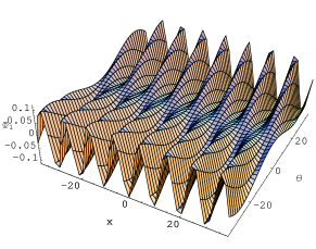
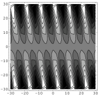
Figure 4. Real part of one-periodic wave for $\mathcal{N}=2$ supersymmetric KdV equation with parameters: $\alpha=0.1,$ $\tau=3,\sigma_{1}=0.01$. (a) Perspective view of wave. (b) Overhead view of wave, with contour plot shown.

$(a)\ \ \ \ \ \ \ \ \ \ \ \ \ \ \ \ \ \ \ \ \ \ \ \ \ \ \ \ \$                   $(b)$                              
             

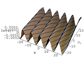
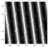
Figure 5. Imaginary part of one-periodic wave for $\mathcal{N}=2$ supersymmetric KdV equation with parameters: $\alpha=0.1,$ $\tau=3,\sigma_{1}=0.01$. (a) Perspective view of wave. (b) Overhead view of wave, with contour plot shown.

$(a)\ \ \ \ \ \ \ \ \ \ \ \ \ \ \ \ \ \ \ \ \ \ \ \ \ \ \ \ \$                   $(b)$                              
             

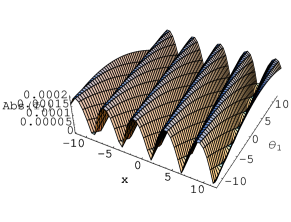
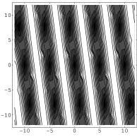
Figure 6. Modulus of one-periodic wave for $\mathcal{N}=2$ supersymmetric KdV equation with parameters: $\alpha=0.1,$ $\tau=3,\sigma_{1}=0.01$. (a) Perspective view of wave. (b) Overhead view of wave, with contour plot shown.

In the following, we further consider asymptotic properties of the one-periodic wave solution. The relation between the one-periodic wave solution (5.12) and the one-soliton solution (5.5) can be established as follows.

Theorem 5. Suppose that $\omega$ and $c$ are given by (5.11). In the one-periodic wave solution (5.12), we choose parameters as

$(5.13)$ $$\gamma=0,\ \ \alpha=\frac{p}{2\pi i},\ \ \beta=\frac{q}{2\pi i},\ \ \delta=\frac{r+\pi\tau}{2\pi i},$$

where the $p,q$ and $r$ are the same as those in (5.5). Then we have the following asymptotic properties

$$c\longrightarrow 0,\ \ \xi\longrightarrow\frac{\eta+\pi\tau}{2\pi i},\ \ f\longrightarrow 1+e^{\eta},\ \ g\longrightarrow 1-e^{\eta},\ \ {\rm as}\ \ \lambda\rightarrow 0.$$

In other words, the one-periodic solution (5.12) tends to the one-soliton solution (5.5) under a small amplitude limit , that is,

$(5.14)$ $$\phi\longrightarrow\phi_{1},\ \ {\rm as}\ \ \lambda\rightarrow 0.$$

Proof. Here we will directly use the system (5.10) to analyze asymptotic properties of one-periodic solution (5.12). We explicitly expand the coefficients of system (5.10) as follows

$(5.15)$ $\displaystyle\vartheta_{1}^{\prime}=-4\pi\lambda+12\pi\lambda^{9}+\cdots,\quad\vartheta_{1}^{\prime\prime\prime}=16\pi^{3}\lambda+432\pi^{3}\lambda^{9}+\cdots,$

$$\vartheta_{2}=-2+2\lambda^{4}+\cdots,\quad\vartheta_{2}^{\prime\prime}=32\pi^{2}\lambda^{4}+\cdots,$$

$$\vartheta_{2}^{(4)}=512\pi^{4}\lambda^{4}+\cdots$$

Suppose that the solution of the system (5.10) is of the form

$(5.16)$ $\displaystyle\omega=\omega_{0}+\omega_{1}\lambda+\omega_{2}\lambda^{2}+\cdots=\omega_{0}+o(\lambda),$

$$c=c_{0}+c_{1}\lambda+c_{2}\lambda^{2}+\cdots=c_{0}+o(\lambda).$$

Substituting the expansions (5.15) and (5.16) into the system (5.11) and letting $\lambda\longrightarrow 0$, we immediately obtain the following relations

$$-4\pi\omega_{0}+16\pi^{3}\alpha^{3}=0,\ \ c_{0}=0,$$

which has a solution

$(5.17)$ $$c_{0}=0,\ \ w_{0}=4\pi^{2}\alpha^{3}.$$

Combining (5.13) and (5.17) leads to

$$c\longrightarrow 0,\ \ 2\pi i\omega\longrightarrow 8\pi^{3}i\alpha^{3}=-p^{3},\ \ {\rm as}\ \ \lambda\rightarrow 0,$$

or equivalently

$(5.18)$ $\displaystyle\hat{\xi}=2\pi i\xi-\pi\tau=px+2\pi i\omega t+q\theta_{1}\sigma+r$

$$\quad\longrightarrow px-p^{3}t+q\theta_{1}\sigma+r=\eta,\ \ {\rm as}\ \ \lambda\rightarrow 0.$$

It remains to identify that the one-periodic wave (5.12) possesses the same form with the one-soliton solution (5.5) under the limit $\lambda\rightarrow 0$. For this purpose, we start to expand the functions $f$ and $g$ in the form

$$f=1+\lambda^{2}(e^{2\pi i\xi}+e^{-2\pi i\xi})+\lambda^{8}(e^{4\pi i\xi}+e^{-4\pi i\xi})+\cdots.$$

$$g=1-\lambda^{2}(e^{2\pi i\xi}+e^{-2\pi i\xi})+\lambda^{8}(e^{4\pi i\xi}+e^{-4\pi i\xi})+\cdots.$$

By using (5.13) and (5.17), it follows that

$(5.19)$ $\displaystyle f=1+e^{\hat{\xi}}+\lambda^{4}(e^{-\hat{\xi}}+e^{2\hat{\xi}})+\lambda^{12}(e^{-2\hat{\xi}}+e^{3\hat{\xi}})+\cdots$

$$\quad\longrightarrow 1+e^{\hat{\xi}}\longrightarrow 1+e^{\eta},\ \ {\rm as}\ \ \lambda\rightarrow 0;$$

$$g=1-e^{\hat{\xi}}+\lambda^{4}(e^{2\hat{\xi}}-e^{-\hat{\xi}})+\lambda^{12}(e^{-2\hat{\xi}}-e^{3\hat{\xi}})+\cdots$$

$$\quad\longrightarrow 1-e^{\hat{\xi}}\longrightarrow 1-e^{\eta},\ \ {\rm as}\ \ \lambda\rightarrow 0.$$

The expression (5.13) follows from (5.19), and thus we conclude that the one-periodic solution (5.12) just goes to the one-soliton solution (5.5) as the amplitude $\lambda\rightarrow 0$. $\square$
4.2. Two-periodic waves and asymptotic properties

We now consider two-periodic wave solutions to the supersymmetric KdV equation (5.2). For the case when $N=2,\ \boldsymbol{s}=\boldsymbol{0},\ \boldsymbol{\varepsilon}=\boldsymbol{1/2}=(1/2,1/2)$ in the Riemann theta function (3.2), we choose $f$ and $g$ to be

$(5.20)$ $\displaystyle f=\vartheta(\boldsymbol{\xi},\boldsymbol{0},\boldsymbol{0}|\boldsymbol{\tau})=\sum_{\boldsymbol{n}\in\mathbb{Z}^{2}}\exp\{2\pi i\langle\boldsymbol{\xi},\boldsymbol{n}\rangle-\pi\langle\boldsymbol{\tau}\boldsymbol{n},\boldsymbol{n}\rangle\},$

$$g=\vartheta(\boldsymbol{\xi},\boldsymbol{1/2},\boldsymbol{0}|\boldsymbol{\tau})=\sum_{\boldsymbol{n}\in\mathbb{Z}^{2}}\exp\{2\pi i\langle\boldsymbol{\xi}+\boldsymbol{1/2},\boldsymbol{n}\rangle-\pi\langle\boldsymbol{\tau}\boldsymbol{n},\boldsymbol{n}\rangle\}$$

$$\ \ =\sum_{\boldsymbol{n}\in\mathbb{Z}^{2}}(-1)^{n_{1}+n_{2}}\exp\{2\pi i\langle\boldsymbol{\xi},\boldsymbol{n}\rangle-\pi\langle\boldsymbol{\tau}\boldsymbol{n},\boldsymbol{n}\rangle\}$$

where we denote $\boldsymbol{n}=(n_{1},n_{2})\in Z^{2},\ \ \boldsymbol{\xi}=(\xi_{1},\xi_{2})\in\mathcal{C}^{2},\ \ \xi_{i}=\alpha_{j}x+\omega_{j}t+\beta_{j}\theta_{1}\sigma+\delta_{j},\ \ j=1,2$, and $\boldsymbol{\alpha}=(\alpha_{1},\alpha_{2}),\ \boldsymbol{\omega}=(\omega_{1},\omega_{2}),\ \boldsymbol{\beta}=(\beta_{1},\beta_{2})\in\mathcal{C}^{2},$; The matrix $\boldsymbol{\tau}$ is a positive definite and real-valued symmetric ${2\times 2}$ matrix, which can take the form

$$\boldsymbol{\tau}=(\tau_{ij})_{2\times 2},\ \ \tau_{12}=\tau_{21},\ \ \tau_{11}>0,\ \ \tau_{22}>0,\ \ \tau_{11}\tau_{22}-\tau_{12}^{2}>0.$$

According to Theorem 5, constraint equations associated with $F(D_{t},D_{x})$ vanish automatically for $(\mu_{1},\mu_{2})=(0,0),(1,1)$, and the constraint equations associated with $G(S_{x},D_{t},D_{x})$ vanish automatically for $(\mu_{1},\mu_{2})=(1,0),(0,1)$. Hence, making the theta functions $f$ and $g$ satisfy the bilinear equation (5.4) gives to the following constraint equations

$(5.21)$ $\displaystyle\sum_{n_{1},n_{2}\in\mathbb{Z}}\left[2\pi i\langle 2\boldsymbol{n}-\boldsymbol{\mu},\boldsymbol{\omega}\rangle-8\pi^{3}i\langle 2\boldsymbol{n}-\boldsymbol{\mu},\boldsymbol{\alpha}\rangle^{3}\right]\exp\{-2\pi\langle\boldsymbol{\tau}(\boldsymbol{n}-\boldsymbol{\mu}/2),\boldsymbol{n}-\boldsymbol{\mu}/2\rangle$

$$+\pi i\sum_{j=1}^{2}(n_{j}-\mu_{j}/2)\}|_{\boldsymbol{\mu}=(\mu_{1},\mu_{2})}=0,\ \ {\rm for}\ \ (\mu_{1},\mu_{2})=(0,1),\ (1,0).$$

and

$(5.22)$ $\displaystyle\sum_{n_{1},n_{2}\in\mathbb{Z}}[-4\pi^{2}\langle 2\boldsymbol{n}-\boldsymbol{\mu},\sigma\boldsymbol{\beta}+\theta_{1}\boldsymbol{\alpha}\rangle\langle 2\boldsymbol{n}-\boldsymbol{\mu},\boldsymbol{\omega}\rangle+16\pi^{4}\langle 2\boldsymbol{n}-\boldsymbol{\mu},\sigma\boldsymbol{\beta}+\theta_{1}\boldsymbol{\alpha}\rangle\langle 2\boldsymbol{n}-\boldsymbol{\mu},\boldsymbol{\alpha}\rangle^{3}$

$$\ \ \ \ -4\pi^{2}\langle 2\boldsymbol{n}-\boldsymbol{\mu},\boldsymbol{\alpha}\rangle^{2}v_{0}+c]\exp\{-2\pi\langle\boldsymbol{\tau}(\boldsymbol{n}-\boldsymbol{\mu}/2),\boldsymbol{n}-\boldsymbol{\mu}/2\rangle$$

$$\ \ \ \ +\pi i\sum_{j=1}^{2}(n_{j}-\mu_{j}/2)\}|_{\boldsymbol{\mu}=(\mu_{1},\mu_{2})}=0,\ \ {\rm for}\ \ (\mu_{1},\mu_{2})=(0,0),\ (1,1).$$

Next, introducing the following notations

$$\lambda_{kl}=e^{-\pi\tau_{kl}/2},k,l=1,2,\boldsymbol{\lambda}=(\lambda_{11},\lambda_{12},\lambda_{22})$$

$$\vartheta_{j}(\boldsymbol{\xi},\boldsymbol{\lambda})=\vartheta(2\xi,\boldsymbol{1/4},-\boldsymbol{s}_{j}/2|2\tau)=\sum_{n_{1},n_{2}\in Z}\exp\{4\pi i\langle\boldsymbol{\xi}+\boldsymbol{1/4},\boldsymbol{n}-\boldsymbol{s_{j}}/2\rangle\}\prod_{k,l=1}^{2}\lambda_{kl}^{(2n_{k}-s_{j,k})(2n_{j}-s_{j,l})},$$

$$\boldsymbol{s_{j}}=(s_{j,1},s_{j,2}),\quad j=1,2,3,4,\ \ \boldsymbol{s_{1}}=(0,1),\ \ \boldsymbol{s_{2}}=(1,0),\ \ \boldsymbol{s_{3}}=(0,0),\ \ \boldsymbol{s_{4}}=(1,1),$$

then by using (3.15), the system (5.21) and (5.22) can be written as a linear system

$(5.23)$ $\displaystyle(\boldsymbol{\omega}\cdot\nabla)\vartheta_{j}(0,\boldsymbol{\lambda})+(\boldsymbol{\alpha}\cdot\nabla)^{3}\vartheta_{j}(0,\boldsymbol{\lambda})=0,\ j=1,2,$

$$[(\sigma\boldsymbol{\beta}+\theta_{1}\boldsymbol{\alpha})\cdot\nabla](\boldsymbol{\omega}\cdot\nabla)\vartheta_{j}(0,\boldsymbol{\lambda})+[(\sigma\boldsymbol{\beta}+\theta_{1}\boldsymbol{\alpha})\cdot\nabla](\boldsymbol{\alpha}\cdot\nabla)^{3}\vartheta_{j}(0,\boldsymbol{\lambda})$$

$$+(\boldsymbol{\alpha}\cdot\nabla)^{2}\vartheta_{j}(0,\boldsymbol{\lambda})v_{0}+\vartheta_{j}(0,\boldsymbol{\lambda})c=0,\ j=3,4.$$

This system can be solved in such a way: After we obtain $\omega,_{1},\omega_{2}$ form the first two equations, We substitute them into last two equations to get $v_{0},c$. With the solution $(\omega_{1},\omega_{2},v_{0},c)$, we get a two-periodic wave solution to the supersymmetric equation (5.2)

$(5.24)$ $$\phi=i\partial_{x}\ln\frac{\vartheta(\boldsymbol{\xi},\boldsymbol{0},\boldsymbol{0}|\boldsymbol{\tau})}{\vartheta(\boldsymbol{\xi},\boldsymbol{1/2},\boldsymbol{0}|\boldsymbol{\tau})}+\theta_{2}\{v_{0}-\partial_{x}\mathfrak{D}\ln[\vartheta(\boldsymbol{\xi},\boldsymbol{0},\boldsymbol{0}|\boldsymbol{\tau})\vartheta(\boldsymbol{\xi},\boldsymbol{1/2},\boldsymbol{0}|\boldsymbol{\tau})]\},$$

where parameters $\omega_{1},\omega_{2},v_{0}$ and $c$ are given by (5.22), while other parameters $\sigma_{1},\sigma_{2},\alpha_{1},$ $\alpha_{2},\tau_{11}$, $\tau_{22},\tau_{12},\delta_{1}$ and $\delta_{2}$ are free.

In summary, the two-periodic wave (5.24), which is a direct generalization of one-periodic waves, has the following features:

(i) Its surface pattern is two-dimensional, namely, there are two phase variables $\xi_{1}$ and $\xi_{2}$. It has $4$ fundamental periods $\{e_{1},e_{2}\}$ and $\{i\tau_{1},i\tau_{2}\}$ in $(\xi_{1},\xi_{2})$, and is spatially periodic in two directions $\xi_{1},\xi_{2}$. Its real part is not periodic in $\theta$ direction, while its real part, imaginary part and modulus are all periodic in $x$ and $t$ directions.

(iii) There is also an influencing band among the Real part of two-periodic waves for the supersymmetric KdV equation under the presence of the Grassmann variable ( see Figure 7 ).

(iv) It was not found that influencing band appears among the imaginary part and modulus of two-periodic waves to the supersymmetric KdV equation ( see Figures 8 and 9 ).

$(a)\ \ \ \ \ \ \ \ \ \ \ \ \ \ \ \ \ \ \ \ \ \ \ \ \ \ \ \ \$                   $(b)$                              
             

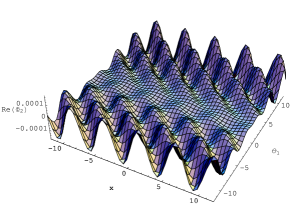
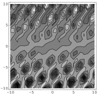
Figure 7. Real part of two-periodic wave for $\mathcal{N}=2$ supersymmetric KdV equation with parameters: $\alpha_{1}=0.1,\ \alpha_{2}=0.2$ $\tau_{11}=3,\ \tau_{12}=0.2,\tau_{22}=3,\sigma_{1}=0.2,\ \sigma_{2}=-0.1$. (a) Perspective view of wave. (b) Overhead view of wave, with contour plot shown.

$(a)\ \ \ \ \ \ \ \ \ \ \ \ \ \ \ \ \ \ \ \ \ \ \ \ \ \ \ \ \$                   $(b)$                              
             

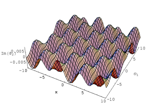
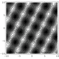
Figure 8. Imaginary part of two-periodic wave for $\mathcal{N}=2$ supersymmetric KdV equation with parameters: $\alpha_{1}=0.1,\ \alpha_{2}=0.2$ $\tau_{11}=3,\ \tau_{12}=0.2,\tau_{22}=3,\sigma_{1}=0.2,\ \sigma_{2}=-0.1$. (a) Perspective view of wave. (b) Overhead view of wave, with contour plot shown.

$(a)\ \ \ \ \ \ \ \ \ \ \ \ \ \ \ \ \ \ \ \ \ \ \ \ \ \ \ \ \$                   $(b)$                              
             

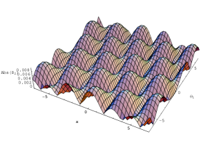
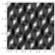
Figure 9. Modulus of two-periodic wave for $\mathcal{N}=2$ supersymmetric KdV equation with parameters: $\alpha_{1}=0.1,\ \alpha_{2}=0.2$ $\tau_{11}=3,\ \tau_{12}=0.2,\tau_{22}=3,\sigma_{1}=0.2,\ \sigma_{2}=-0.1$. (a) Perspective view of wave. (b) Overhead view of wave, with contour plot shown.

Finally, we consider the asymptotic properties of the two-periodic solution (5.24). In a similar way to Theorem 5, we can establish the relation between the two-periodic solution (5.24) and the two-soliton solution (5.6) as follows.

Theorem 6. Assume that $(\omega_{1},\omega_{2},v_{0},c)$ is a solution of the system (5.23). In the two-periodic wave solution (5.24), a choice of parameters is given by

$(5.25)$ $\displaystyle\alpha_{j}=\frac{p_{j}}{2\pi i},\ \ \beta_{j}=\frac{q_{j}}{2\pi i},\ \ \delta_{j}=\frac{r_{j}+\pi\tau_{jj}}{2\pi i},\ \ \tau_{12}=-\frac{A_{12}}{2\pi},\ \ j=1,2,$

with the $p_{j},q_{j},r_{j}\in\Lambda_{0},j=1,2$ and $A_{12}$ as those given in (5.6). Then under the constraint $\alpha_{1}\beta_{2}=\alpha_{2}\beta_{1}$, we have the following asymptotic relations

$(5.26)$ $\displaystyle v_{0}\longrightarrow 0,\ \ \ c\longrightarrow 0,\ \ \xi_{j}\longrightarrow\frac{\eta_{j}+\pi\tau_{jj}}{2\pi i},\ \ j=1,2,$

$$f\longrightarrow 1+e^{\eta_{1}}+e^{\eta_{2}}+e^{\eta_{1}+\eta_{2}+A_{12}},\ \ g\longrightarrow 1-e^{\eta_{1}}-e^{\eta_{2}}+e^{\eta_{1}+\eta_{2}+A_{12}},$$

$$\ \ \ {\rm as}\ \ \lambda_{11},\lambda_{22}\rightarrow 0.$$

So the two-periodic wave solution (5.24) just tends to the two-soliton solution (5.6) under a certain limit

$$\phi\longrightarrow\phi_{2},\ \ {\rm as}\ \ \lambda_{11},\lambda_{22}\rightarrow 0.$$

Proof. From (5.25), the constraint $\alpha_{1}\beta_{2}=\alpha_{2}\beta_{1}$ leads to $p_{1}q_{2}-p_{2}q_{1}=0$, which implies that $\tau_{12}=-A_{12}/2\pi$ is independent of Grassmann variable $\theta$ according to (5.7).

Using (5.20), we explicitly expand the functions $f$ and $g$ in the following form

$$f=1+(e^{2\pi i\xi_{1}}+e^{-2\pi i\xi_{1}})e^{-\pi\tau_{11}}+(e^{2\pi i\xi_{2}}+e^{-2\pi i\xi_{2}})e^{-\pi\tau_{22}}$$

$$\ \ \ \ \ \ +(e^{2\pi i(\xi_{1}+\xi_{2})}+e^{-2\pi i(\xi_{1}+\xi_{2})})e^{-\pi(\tau_{11}+2\tau_{12}+\tau_{22})}+\cdots$$

$$g=1-(e^{2\pi i\xi_{1}}+e^{-2\pi i\xi_{1}})e^{-\pi\tau_{11}}-(e^{2\pi i\xi_{2}}+e^{-2\pi i\xi_{2}})e^{-\pi\tau_{22}}$$

$$\ \ \ \ \ \ +(e^{2\pi i(\xi_{1}+\xi_{2})}+e^{-2\pi i(\xi_{1}+\xi_{2})})e^{-\pi(\tau_{11}+2\tau_{12}+\tau_{22})}+\cdots$$

Further using (4.5) and making a transformation $\hat{\omega}_{j}=2\pi i\omega_{j},j=1,2$, we infer that

$$f=1+e^{\hat{\xi}_{1}}+e^{\hat{\xi}_{2}}+e^{\hat{\xi}_{1}+\hat{\xi}_{2}-2\pi\tau_{12}}+\lambda_{11}^{4}e^{-\hat{\xi}_{1}}+\lambda_{22}^{4}e^{-\hat{\xi}_{2}}+\lambda_{11}^{4}\lambda_{22}^{4}e^{-\hat{\xi}_{1}-\hat{\xi}_{2}-2\pi\tau_{12}}+\cdots$$

$$\ \ \ \ \ \longrightarrow 1+e^{\hat{\xi}_{1}}+e^{\hat{\xi}_{2}}+e^{\hat{\xi}_{1}+\hat{\xi}_{2}+A_{12}},\ \ {\rm as}\ \ \lambda_{11},\lambda_{22}\rightarrow 0,$$

$$g=1-e^{\hat{\xi}_{1}}-e^{\hat{\xi}_{2}}+e^{\hat{\xi}_{1}+\hat{\xi}_{2}-2\pi\tau_{12}}-\lambda_{11}^{4}e^{-\hat{\xi}_{1}}-\lambda_{22}^{4}e^{-\hat{\xi}_{2}}+\lambda_{11}^{4}\lambda_{22}^{4}e^{-\hat{\xi}_{1}-\hat{\xi}_{2}-2\pi\tau_{12}}+\cdots$$

$$\ \ \ \ \ \longrightarrow 1-e^{\hat{\xi}_{1}}-e^{\hat{\xi}_{2}}+e^{\hat{\xi}_{1}+\hat{\xi}_{2}+A_{12}},\ \ {\rm as}\ \ \lambda_{11},\lambda_{22}\rightarrow 0,$$

where $\hat{\xi}_{j}=p_{j}x+\hat{\omega}_{j}t+q_{j}\theta_{1}\sigma+r_{j},\ \ j=1,2.$

It remains to prove that

$(5.27)$ $\displaystyle c\longrightarrow 0,\ \ \ \hat{\omega}_{j}\longrightarrow-p_{j}^{3},\ \ \hat{\xi}_{j}\longrightarrow\eta_{j},\ \ j=1,2,\ \ \ {\rm as}\ \ \lambda_{11},\lambda_{22}\rightarrow 0.$

As in the case when $N=1$, we let the solution of the system (5.23) be the form

$(5.28)$ $\displaystyle\omega_{1}=\omega_{1,0}+\omega_{1,1}\lambda_{11}+\omega_{2,2}\lambda_{22}+o(\lambda_{11},\lambda_{22}),$

$$\omega_{2}=\omega_{2,0}+\omega_{2,1}\lambda_{11}+\omega_{2,2}\lambda_{22}+o(\lambda_{11},\lambda_{22}),$$

$$v_{0}=v_{0,0}+v_{0,1}\lambda_{11}+v_{0,2}\lambda_{22}+o(\lambda_{11},\lambda_{22}),$$

$$c=c_{0}+c_{1}\lambda_{11}+c_{2}\lambda_{22}+o(\lambda_{11},\lambda_{22}).$$

Expanding functions $\vartheta_{j},j=1,2,3,4$ in the system (5.23), together with substitution of assumption (5.28), the second and third equation is divided by $\lambda_{11}$ and $\lambda_{22}$, respectively; the fourth equation is divided by $\lambda_{11}\lambda_{22}$, and letting $v_{0,0}=0,\ \lambda_{11},\lambda_{22}\longrightarrow 0$ , we then obtain

$(5.29)$ $\displaystyle c_{0}=0,$

$$-8\pi\omega_{1,0}+32\pi^{4}\alpha_{1}^{3}=0,$$

$$-8\pi\omega_{2,0}+32\pi^{4}\alpha_{2}^{3}=0,$$

$$[-8\pi^{2}(\omega_{1,0}+\omega_{2,0})+32\pi^{4}(\alpha_{1}+\alpha_{2})^{3}]\lambda_{12}$$

$$\ \ \ \ +[-8\pi^{2}(\omega_{1,0}-\omega_{2,0})+32\pi^{4}(\alpha_{1}-\alpha_{2})^{3}]\lambda_{12}^{-1}=0.$$

The first three equations in the system (5.9) have a solution

$(5.30)$ $\displaystyle c_{0}=0,\ \ v_{0,0}=0,\ \ \omega_{1,0}=4\pi^{2}\alpha_{1}^{3},\ \ \omega_{2,0}=4\pi^{2}\alpha_{2}^{3},$

The fourth equation in the system (5.29) satisfied automatically by using (5.25) and (5.30), thus we have

$(5.31)$ $\displaystyle c_{0}=c_{1}=c_{2}=0,\ \ v_{0,0}=0,\ \ \omega_{1,0}=4\pi^{2}\alpha_{1}^{3},\ \ \omega_{2,0}=4\pi^{2}\alpha_{2}^{3}.$

Using (5.28) and (5.31), we conclude that

$$v_{0}=o(\lambda_{11},\lambda_{22})\longrightarrow 0,\ \ c=o(\lambda_{11},\lambda_{22})\longrightarrow 0,\ \ \omega_{1}=4\pi^{2}\alpha_{1}^{3}+o(\lambda_{11},\lambda_{22})\longrightarrow 4\pi^{2}\alpha_{1}^{3},$$

$$\omega_{2}=4\pi^{2}\alpha_{2}^{3}+o(\lambda_{11},\lambda_{22})\longrightarrow 4\pi^{2}\alpha_{2}^{3},\ \ \ {\rm as}\ \ \lambda_{11},\lambda_{22}\rightarrow 0,$$

and therefore we have (5.26). So the two-periodic wave solution (5.23) tends to the two-supersoliton solution (5.6) as $\lambda_{11},\lambda_{22}\rightarrow 0$. $\square$
6. Conclusion and future work

Following the procedure described in this paper, we are able to construct quasi-periodic wave solutions for other supersymmetric equations also can be dealt with by the same way. For instance,

(1) Supersymmetric KdV equation [40, 42, 43]

$$\Phi_{t}+3\left(\Phi\mathfrak{D}\Phi\right)_{x}+\Phi_{xxx}=0,$$

(2) Supersymmetric MKdV equation [41, 49, 65]

$$\phi_{t}-3\phi\mathfrak{D}(\phi_{x})\mathfrak{D}\phi-3(\mathfrak{D}\phi)^{2}\phi_{x}+\phi_{xxx}=0,$$

(3)  Supersymmetric It’s equation [66]

$$\mathfrak{D}_{t}F_{t}+6(F_{x}(\mathfrak{D}_{t}F))_{x}+\mathfrak{D}_{t}F_{xxx}=0,$$

(4)  Supersymmetric two-boson equation [67, 68]

$$\phi_{1,t}=\mathfrak{D}((\mathfrak{D}\phi_{1})^{2})+2\phi_{2,x}-\phi_{1,xx},$$

$$\phi_{2,t}=2((\mathfrak{D}\phi_{1})\phi_{2})_{x}+\phi_{2,xx}.$$

The system (3.10) indicates that constructing multi-periodic wave solutions depends on the solvability of the system. We consider the number of constraint equations and some unknown parameters. Obviously, the number of constraint equations of the type (3.10) is $2^{N}$. On the other hand we have parameters $\tau_{ii},\tau_{ij},\alpha_{i},\omega_{i},\phi_{0},c$, whose total number is $\frac{1}{2}N(N+1)+3N+2$. Among them, $2N$ parameters $\tau_{ii},\omega_{i}$ are taken to be the given parameters related to the amplitudes and wave numbers of $N$-periodic waves. Hence, the number of the unknown parameters is $\frac{1}{2}N(N+1)+N+2$. while $\frac{1}{2}N(N+1)$ parameters $\tau_{ij}$ implicitly appear in series form, which is general can not to be solved explicit. Hence, the number of the explicit unknown parameters is only $N+2$. The number of equations is larger than the unknown parameters in the case when $N>2$. This fact means that if equation (3.10) is satisfied by the unknowns, we have at least $N$-periodic wave solutions ($N\leq 2$). It is still possible to construct multi-periodic wave solutions for $N\geq 3$ by adding the number of parameters (for example, using constant solution and integration constant) or decreasing the number of equations (for example, using odd and even properties of considered equations). In this paper, we consider one-periodic wave solution of the equation (1.2), which belongs to the cases when $N=1$ and $N=2$ in the Riemann theta function (3.1). There are still certain difficulties in the calculation for the case $N\geq 3$.

We expect the proposed method to be extended to $\mathcal{N}=1$ supersymmetric sine-Gordon equation and $\mathcal{N}=1$ supersymmetric KP equation, as well as other discrete supersymmetric equations (like supersymmetric Toda lattice). For the $\mathcal{N}=2$ supersymmetric equations with ordinary variables $x,t$ and Grassmann variables $\theta_{1},\theta_{2}$, their corresponding superspace is $\mathbb{R}_{\Lambda}^{2,2}=\Lambda_{0}^{2}\times\Lambda_{1}^{2}$. In this case, the Grassmann algebra $G_{2}(\sigma_{1},\sigma_{2})$ whose dimension is four. The $\tau$ matrix will be dependent on the odd parameters $\sigma_{1},\sigma_{2}$. In superspace $\mathbb{R}_{\Lambda}^{2,2}$, the super bilinear forms of $\mathcal{N}=2$ supersymmetric equations, their quasi-periodic solutions and asymptotic properties remain open. We intend to return to these question in some future publications.
Acknowledgment

The work described in this paper was supported by grants from the National Science Foundation of China (No.10971031), Shanghai Shuguang Tracking Project (No.08GG01) and Innovation Program of Shanghai Municipal Education Commission (No.10ZZ131).

References

[1]
[2] S. P. Novikov, Funct. Anal. Appl. 8(1974): 236-246.
[3] B. A. Dubrovin, Funct. Anal. Appl. 9(1975): 265-277.
[4] A. Its and V. Matveev, Funct. Anal. Appl. 9(1975): 65-66.
[5] P. D. Lax, Comm. Pure Appl. 28(1975): 141-188.
[6] H. P. Mckean and P. Moerbeke, Invent. Math. 30(1975): 217-274.
[7] E. Belokolos, A. Bobenko, V. Enol’skij, A. Its and V. Matveev,
Algebro-Geometrical Approach to Nonlinear Integrable
Equations ( Springer, Berlin, 1994).
[8] F. Gesztesy and H. Holden, Soliton Equations and Their Algebro-Geometric Solutions,
(Cambridge University Press, 2003).
[9] F. Gesztesy and H Holden. Phil Trans R Soc A366 (2008): 1025-1054.
[10] Z. J. Qiao, Comm Math Phys, 239 (2003): 309-341.
[11] L. Zampogni, Advanced Nonl Studies, 3 (2007): 345-380.
[12] R. G. Zhou, J. Math. Phys. 38(1997): 2535-2346.
[13] C. W. Cao, Y. T. Wu and X. G. Geng. J. Math. Phys. 40(1999): 3948-3970.
[14] X. G. Geng, Y. T. Wu and C. W. Cao. J. Phys. A 32 (1999): 3733-3742.
[15] X. G. Geng, and C. W. Cao. Nonlinearity, 14 (2001): 1433-1452.
[16] X. G. Geng, H. H. Dai, J. Y. Zhu and H. Y. Wang. Stud. Appl. Math. 118 (2007): 281-312.
[17] Y. C. Hon and E. G. Fan, J. Math.Phys. 46 (2005): 032701-21.
[18] J. Hammack, N. Scheffner and H. Segur, J. Fluid Mech.
209 567-589 (1989)
[19] J. Hammack, D. McCallister, N. Scheffner and H.
Segur, J. Fluid Mech. 285 95-112 (1995)
[20] R. Hirota and J. Satsuma: Prog. Theor. Phys. 57 (1977) 797.
[21] R. Hirota: Direct methods in soliton theory (Springer-verlag, Berlin, 2004).
[22] X. B. Hu and P. A. Clarkson, J. Phys. A 28 (1995) 5009.
[23] X. B. Hu, C X Li, J. J. C. Nimmo and G. F. Yu, J. Phys. A,
38 (2005) 195.
[24] R Hirota and Y. Ohta: J. Phys. Soc. Jpn. 60 (1991)
798.
[25] D. J. Zhang, J. Phys. Soc. Jpn. 71 (2002) 2649.
[26] K. Sawada and T Kotera: Prog. Theor. Phys. 51 (1974) 1355.
[27] A. Nakamura, J. Phys. Soc. Jpn. 47, 1701-1705 (1979).
[28] A. Nakamura, J. Phys. Soc. Jpn. 48(1980), 1365.
[29] R. Hirota and M. Ito, J. Phys. Soc. Jpn. 48(1980), 1365.
[30] H. H. Dai, E. G. Fan and X. G. Geng, arxiv.org/pdf/nlin/0602015
[31] Y. Zhang, L. Y. Ye, Y. N. Lv and H. Q. Zhao, J. Phys A, 40 (2007), 5539.
[32] Y. C. Hon, E. G. Fan and Z. Y. Qin, Modern Phys Lett B, 22 (2008), 547.
[33] E. G. Fan and Y. C. Hon, Phys Rev E, 78 (2008), 036607.
[34] E. G. Fan, J. Phys A, 42 (2009), 095206.
[35] W. X. Ma, R. G. Zhou, J. Math. Phys, 24 (2009), 1677.
[36] P. Ramond, Phys. Rev. D, 3 (1971), 2415.
[37] A. Neveu and J. H. Schwarz, Nucl. Phys. B, 31 (1971), 86.
[38] J. Wess and B. Zumino, Nucl. Phys. B, 70 (1974), 39.
[39] F. A. Berezin, Introduction to super-Analysi, Dordrecht: Reidel, 1987.
[40] Yu. I. Manin and A. O. Radul, Commun. Math. Phys. 98 (1985), 65.
[41] P. Mathieu, J. Math. Phys. 29 (1988), 2499.
[42] W. Oevel and Z. Popowicz, Commun. Math. Phys. 139 (1991), 441.
[43] A. S. Carstea, Nonlinearity 13 (2000), 1645.
[44] A. S. Carstea, A. Ramani and B Grammaticos, Nonlinearity 14 (2000), 1419.
[45] D. Sarma, Nucl. Phys. B 681 (2004), 351.
[46] Q. P. Liu, Lett Math. Phys. 35 (1995), 115.
[47] Q. P. Liu and Y. F. Xie, Phys. Lett. A 325 (2004), 139.
[48] Q. P. Liu and X. B. Hu, J. Phys. A 38 (2005), 6371.
[49] Q. P. Liu, X. B. Hu and M. X. Zhang, Nonlinearity 18 (2005), 1597.
[50] S. Ghosh, J. Nonl. Math. Phys. 10 (2003), 526.
[51] V. S. Vladimirov, Theor. Math. Phys. 59 (1984), 3.
[52] V. S. Vladimirov, Theor. Math. Phys. 60 (1984),
169.
[53] D. Mumford, Tata Lectures on Theta II Progress in Mathmatics,
Vol. 43 ( Boston: Birkhäuser, 1984).
[54] R. Hirota and M Ito, J. Phys. Soc. Jpn. 52 (1983) 744
[55] K. Konno, J. Phys. Soc. Jpn. 61 (1992) 51
[56] Y. X. Yu, Commun. Theor. Phys. 49 (2008), 685.
[57] K. Tian and Q. P. Liu, Phys. Lett. A 373 (2009), 169.
[58] C. A. Laberge, P. Mathieu, Phys. Lett. B 215 (1988), 718.
[59] C. A. Laberge, P. Mathieu, J. Math. Phys. 32 (1991), 923.
[60] M. X. Zhang, Q. P. Liu, Y. L. Shen and K. Wu, Sic. in China. 52 (2009), 1973.
[61] Z. Popowicz. Phys. Lett. A 174 (1993), 411.
[62] S. Bourque and P. Mathieu, J. Math. Phys. 42 (2001), 3517.
[63] T. Inami and H. Kanno, Nuclear Phys. B 359 (1991), 201.
[64] Q. P. Liu and Y. F. Xie, Phys. Lett. A 235 (1997), 335.
[65] S. Ghosh and D. Sarma, Nonlinearity, 16 (2003), 411.
[66] S. Q. Liu, X. B. Hu and Q. P. Liu, J. Phys. Soc. Jpn 75 (2006),
064004.
[67] J. C. Brunelli, A. Das, Phys. Lett. B, 337 (1994),
303.
[68] Q. P. Liu, X. X. Yang, Phys. Phys A. 351 (2006), 131.