Adaptive Numerical Treatment of
Elliptic Systems on Manifolds

Abstract.

Adaptive multilevel finite element methods are developed and analyzed for certain elliptic systems arising in geometric analysis and general relativity. This class of nonlinear elliptic systems of tensor equations on manifolds is first reviewed, and then adaptive multilevel finite element methods for approximating solutions to this class of problems are considered in some detail. Two a posteriori error indicators are derived, based on local residuals and on global linearized adjoint or dual problems. The design of Manifold Code (MC) is then discussed; MC is an adaptive multilevel finite element software package for 2- and 3-manifolds developed over several years at Caltech and UC San Diego. It employs a posteriori error estimation, adaptive simplex subdivision, unstructured algebraic multilevel methods, global inexact Newton methods, and numerical continuation methods for the numerical solution of nonlinear covariant elliptic systems on 2- and 3-manifolds. Some of the more interesting features of MC are described in detail, including some new ideas for topology and geometry representation in simplex meshes, and an unusual partition of unity-based method for exploiting parallel computers. A short example is then given which involves the Hamiltonian and momentum constraints in the Einstein equations, a representative nonlinear 4-component covariant elliptic system on a Riemannian 3-manifold which arises in general relativity. A number of operator properties and solvability results recently established are first summarized, making possible two quasi-optimal a priori error estimates for Galerkin approximations which are then derived. These two results complete the theoretical framework for effective use of adaptive multilevel finite element methods. A sample calculation using the MC software is then presented.

1. Introduction

In this paper we consider adaptive multilevel finite element methods for certain elliptic systems arising in geometric analysis and general relativity. Our interest is in developing adaptive approximation techniques for the highly accurate and efficient numerical solution of this class of problems. We begin by giving a brief introduction to this class of nonlinear elliptic systems of tensor equations on manifolds, and then discuss adaptive multilevel finite element methods for approximating solutions to this class of problems. We derive two a posteriori error indicators, the first of which is local residual-based, whereas the second is based on a global linearized adjoint or dual problem.

The design of a computer program called Manifold Code (MC) is then described, which is an adaptive multilevel finite element software package for partial differential equations (PDEs) on 2- and 3-manifolds developed over several years at Caltech and UC San Diego. MC employs a posteriori error estimation, adaptive simplex subdivision, unstructured algebraic multilevel methods, global inexact Newton methods, and numerical continuation methods for the accurate and efficient numerical solution of nonlinear covariant elliptic systems on 2- and 3-manifolds. We describe some of the more interesting features of MC in detail, including some new ideas for topology and geometry representation in simplex meshes. We also describe an unusual partition of unity-based method in MC for using parallel computers in an adaptive setting, based on joint work with R. Bank [9]. Global $L^{2}$- and $H^{1}$-error estimates are derived for solutions produced by MC’s parallel algorithm by using Babuška and Melenk’s Partition of Unity Method (PUM) error analysis framework [5] and by exploiting the recent results of Xu and Zhou on local error estimation [97].

We finish with an example involving the Hamiltonian and momentum constraints in the Einstein equations, a representative nonlinear 4-component covariant elliptic system on a Riemannian 3-manifold which arises in general relativity. We first summarize a number of operator properties and solvability results which were established recently in [56]. We then derive two quasi-optimal a priori error estimates for Galerkin approximations of the constrains, completing the theoretical framework for effective use of adaptive multilevel finite element methods. We then present a sample calculation using the MC software for this application. More detailed examples involving the use of MC for the Einstein constraints may be found in [55, 26]. Applications of MC to problems in other areas such as biology and elasticity can be found in [54, 8, 9].

2. Adaptive Multilevel Finite Element Methods for Nonlinear Elliptic Equations

In this section we will first give an overview of nonlinear elliptic equations on manifolds, followed by a brief description of adaptive multilevel finite element techniques for such equations.

2.1. Nonlinear elliptic equations on manifolds

Let $({\mathcal{M}},g_{ab})$ be a connected compact Riemannian $d$-manifold with boundary $(\partial{\mathcal{M}},\sigma_{ab})$, where the boundary metric $\sigma_{ab}$ is inherited from $g_{ab}$. To allow for general boundary conditions, we will view the boundary $(d-1)$-submanifold $\partial{\mathcal{M}}$ (which we assume to be oriented) as being formed from two disjoint submanifolds $\partial_{0}{\mathcal{M}}$ and $\partial_{1}{\mathcal{M}}$, i.e.,

$$\partial_{0}{\mathcal{M}}\cup\partial_{1}{\mathcal{M}}=\partial{\mathcal{M}},\ \ \ \ \ \ \ \ \partial_{0}{\mathcal{M}}\cap\partial_{1}{\mathcal{M}}=\emptyset.$$ (2.1)

When convenient in the discussions below, one of the two submanifolds $\partial_{0}{\mathcal{M}}$ or $\partial_{1}{\mathcal{M}}$ may be allowed to shrink to zero measure, leaving the other to cover $\partial{\mathcal{M}}$. Moreover, in what follows it will usually be necessary to make smoothness assumptions about the boundary submanifold $\partial{\mathcal{M}}$, such as Lipschitz continuity (for a precise definition see [1]). We will employ the abstract index notation (cf. [92]) and summation convention for tensor expressions below, with indices running from $1$ to $d$ unless otherwise noted. The summation convention is that all repeated symbols in products imply a sum over that index. Partial differentiation on a non-flat manifold must be covariant, meaning that application of gradient and divergence operators require the use of a connection due to the curvilinear nature of the coordinate system used to describe the domain manifold. Christoffel symbols formed with respect to the given metric $g_{ab}$ (at times denoted $\hat{\gamma}_{ab}$) provide default connection coefficients.

Covariant partial differentiation of a tensor $t^{a_{1}\cdots a_{p}}_{~{}~{}~{}~{}~{}~{}~{}b_{1}\cdots b_{q}}$ using the connection provided by the metric $g_{ab}$ will be denoted as $t^{a_{1}\cdots a_{p}}_{~{}~{}~{}~{}~{}~{}~{}b_{1}\cdots b_{q};c}$ or as $D_{c}t^{a_{1}\cdots a_{p}}_{~{}~{}~{}~{}~{}~{}~{}b_{1}\cdots b_{q}}$. Denoting the outward unit normal to $\partial{\mathcal{M}}$ as $n_{b}$, recall the Divergence Theorem for a vector field $w^{b}$ on ${\mathcal{M}}$ (cf. [65]):

$$\int_{{\mathcal{M}}}w^{b}_{~{};b}~{}dx=\int_{\partial{\mathcal{M}}}w^{b}n_{b}~{}ds,$$ (2.2)

where $dx$ denotes the measure on ${\mathcal{M}}$ generated by the volume element of $g_{ab}$:

$$dx=\sqrt{\text{det}~{}g_{ab}}~{}dx^{1}\cdots dx^{d},$$ (2.3)

and where $ds$ denotes the boundary measure on $\partial{\mathcal{M}}$ generated by the boundary volume element of $\sigma_{ab}$. Making the choice $w^{b}=u_{a_{1}\ldots a_{k}}v^{a_{1}\ldots a_{k}b}$ in (2.2) and forming the divergence $w^{b}_{~{};b}$ by applying the product rule leads to a useful integration-by-parts formula for certain contractions of tensors:

$$\int_{{\mathcal{M}}}u_{a_{1}\ldots a_{k}}v^{a_{1}\ldots a_{k}b}_{~{}~{}~{}~{}~{}~{}~{}~{}~{};b}~{}dx = \int_{\partial{\mathcal{M}}}u_{a_{1}\ldots a_{k}}v^{a_{1}\ldots a_{k}b}n_{b}~{}ds$$

$$-\int_{{\mathcal{M}}}v^{a_{1}\ldots a_{k}b}u_{a_{1}\ldots a_{k};b}~{}dx.$$

When $k=0$ this reduces to the familiar case where $u$ and $v$ are scalars.

2.1.1. Coupled elliptic systems and augumented systems

Consider now a general second-order elliptic system of tensor equations in strong divergence form over ${\mathcal{M}}$:

$$-A^{ia}(x^{b},u^{j},u^{k}_{~{};c},\lambda)_{;a}+B^{i}(x^{b},u^{j},u^{k}_{~{};c},\lambda) = 0~{}\text{~{}in~{}}{\mathcal{M}},$$ (2.5)

$$A^{ia}(x^{b},u^{j},u^{k}_{~{};c},\lambda)n_{a}+C^{i}(x^{b},u^{j},u^{k}_{~{};c},\lambda) = 0~{}\text{~{}on~{}}\partial_{1}{\mathcal{M}},$$ (2.6)

$$u^{i}(x^{b}) = E^{i}(x^{b},\lambda)~{}\text{~{}on~{}}\partial_{0}{\mathcal{M}},$$ (2.7)

where

$$\lambda\in{\mathbb{R}}^{m},\ \ \ 1\leq a,b,c\leq d,\ \ \ 1\leq i,j,k\leq n,$$

$$A:{\mathcal{M}}\times{\mathbb{R}}^{n}\times{\mathbb{R}}^{nd}\times{\mathbb{R}}^{m}\mapsto{\mathbb{R}}^{nd},\ \ \ B:{\mathcal{M}}\times{\mathbb{R}}^{n}\times{\mathbb{R}}^{nd}\times{\mathbb{R}}^{m}\mapsto{\mathbb{R}}^{n},$$

$$C:\partial_{1}{\mathcal{M}}\times{\mathbb{R}}^{n}\times{\mathbb{R}}^{nd}\times{\mathbb{R}}^{m}\mapsto{\mathbb{R}}^{n},\ \ \ E:\partial_{0}{\mathcal{M}}\times{\mathbb{R}}^{m}\mapsto{\mathbb{R}}^{n}.$$

The divergence-form system (2.5)–(2.7), together with the boundary conditions, can be viewed as an operator equation of the form

$$G(u,\lambda)=0,\ \ \ \ \ G:{\mathcal{B}}_{1}\times{\mathbb{R}}^{m}\mapsto{\mathcal{B}}_{2}^{*},$$ (2.8)

for some Banach spaces ${\mathcal{B}}_{1}$ and ${\mathcal{B}}_{2}$, where ${\mathcal{B}}_{2}^{*}$ denotes the dual space of ${\mathcal{B}}_{2}$. Analysis and numerical techniques often require the Gateaux-linearization operator $D_{u}G(u)\in{\mathcal{L}}({\mathcal{B}}_{1},{\mathcal{B}}_{2}^{*})$. If $D_{u}G(u_{0},\lambda_{0})$ is a linear homeomorphism from ${\mathcal{B}}_{1}$ to ${\mathcal{B}}_{2}^{*}$, then the Implicit Function Theorem guarantees that there is a neighborhood of $(\lambda_{0},u_{0})\in{\mathbb{R}}^{m}\times{\mathcal{B}}_{1}$ containing regular solutions to (2.8). If $D_{u}G(u_{0},\lambda_{0})$ is singular, so that the Implicit Function Theorem does not apply, then the standard approach is to expand the solution spaces in such a way that the expanded problem has a regular solution. This is called the augmented or bordered system approach to handling folds and bifurcations, and is the basis for sophisticated numerical path-following algorithms [62, 63]. In the case of a simple limit point (or fold), where $D_{u}G(u_{0})$ is a Fredholm operator of ${\mathcal{B}}_{1}$ into ${\mathcal{B}}_{2}^{*}$ with index $m$, then the augmented system approach involves simply adding a set of $m$ linear constraints to the original system, producing:

$$F(u,\lambda,s)=\left[\begin{array}[]{c}G(u,\lambda)\\ N(u,\lambda,s)\end{array}\right]=0,\ \ \ \ F:{\mathcal{B}}_{1}\times{\mathbb{R}}^{m}\times{\mathbb{R}}^{m}\mapsto{\mathcal{B}}_{2}^{*}\times{\mathbb{R}}^{m}.$$ (2.9)

If the augmentation function $N(u,\lambda,s):{\mathcal{B}}_{1}\times{\mathbb{R}}^{m}\times{\mathbb{R}}^{m}\mapsto{\mathbb{R}}^{m}$ is chosen correctly, then the linearization operator $DF\in{\mathcal{L}}({\mathcal{B}}_{1}\times{\mathbb{R}}^{m},{\mathcal{B}}_{2}^{*}\times{\mathbb{R}}^{m})$ for the whole system, which can be written as

$$DF(u,\lambda,s)=\left[\begin{array}[]{ll}D_{u}G(u,\lambda)&D_{\lambda}G(u,\lambda)\\ D_{u}N(u,\lambda,s)&D_{\lambda}N(u,\lambda,s)\\ \end{array}\right],$$ (2.10)

becomes a homeomorphism again.

Our interest here is primarily in coupled systems of one or more scalar field equations and one or more $d$-vector field equations, possibly augmented as in (2.9)–(2.10). The unknown $n$-vector $u^{i}$ then in general consists of $n_{s}$ scalars and $n_{v}$ $d$-vectors, so that $n=n_{s}+n_{v}\cdot d$. To allow the $n$-component system (2.5)–(2.7) to be treated notationally as if it were a single $n$-vector equation, it will be convenient to introduce the following notation for the unknown vector $u^{i}$ and for the metric of the product space of scalar and vector components of $u^{i}$:

$${\mathcal{G}}_{ij}=\left[\begin{array}[]{ccc}g_{ab}^{(1)}&&0\\ &\ddots&\\ 0&&g_{ab}^{(n_{e})}\\ \end{array}\right],~{}~{}~{}~{}~{}~{}u^{i}=\left[\begin{array}[]{c}u^{a}_{(1)}\\ \vdots\\ u^{a}_{(n_{e})}\\ \end{array}\right],~{}~{}~{}~{}~{}n_{e}=n_{s}+n_{v}.$$ (2.11)

If $u^{a}_{(k)}$ is a $d$-vector we take $g_{ab}^{(k)}=g_{ab}$; if $u^{a}_{(k)}$ is a scalar we take $g_{ab}^{(k)}=1$.

2.1.2. Weak formulations

The weak form of (2.5)–(2.7) is obtained by taking the $L^{2}$-based duality pairing between a vector $v^{j}$ (vanishing on $\partial_{0}{\mathcal{M}}$) lying in a product space of scalars and tensors, and the residual of the tensor system (2.5), yielding:

$$\int_{{\mathcal{M}}}{\mathcal{G}}_{ij}\left(B^{i}-A^{ia}_{\ \ ;a}\right)v^{j}~{}dx=0.$$ (2.12)

Due to the definition of ${\mathcal{G}}_{ij}$ in (2.11), this is simply a sum of integrals of scalars, each of which is a contraction of the type appearing on the left side in (2.1). Using then (2.1) and (2.6) together in (2.12), and recalling that $v^{i}=0$ on $\partial_{0}{\mathcal{M}}$ satisfying (2.1), yields

$$\int_{{\mathcal{M}}}{\mathcal{G}}_{ij}A^{ia}v^{j}_{~{};a}~{}dx+\int_{{\mathcal{M}}}{\mathcal{G}}_{ij}B^{i}v^{j}~{}dx+\int_{\partial_{1}{\mathcal{M}}}{\mathcal{G}}_{ij}C^{i}v^{j}~{}ds=0.$$ (2.13)

Equation (2.13) leads to a covariant weak formulation of the problem:

$$\text{Find}~{}u\in\bar{u}+{\mathcal{B}}_{1}~{}\text{s.t.}~{}\langle F(u),v\rangle=0,\ \ \forall~{}v\in{\mathcal{B}}_{2},$$ (2.14)

for suitable Banach spaces of functions ${\mathcal{B}}_{1}$ and ${\mathcal{B}}_{2}$, where the nonlinear weak form $\langle F(\cdot),\cdot\rangle$ can be written as:

$$\langle F(u),v\rangle=\int_{{\mathcal{M}}}{\mathcal{G}}_{ij}(A^{ia}v^{j}_{~{};a}+B^{i}v^{j})~{}dx+\int_{\partial_{1}{\mathcal{M}}}{\mathcal{G}}_{ij}C^{i}v^{j}~{}ds.$$ (2.15)

The notation $\langle w,v\rangle$ will represent the duality pairing of a function $v$ in a Banach space ${\mathcal{B}}$ with a bounded linear functional (or form) $w$ in the dual space ${\mathcal{B}}^{*}$. Depending on the particular function spaces involved, the pairing may be thought of as coinciding with the $L^{2}$-inner-product through the Riesz Representation Theorem [98]. The affine shift tensor $\bar{u}$ in (2.14) represents the essential or Dirichlet part of the boundary condition if there is one; the existence of $\bar{u}$ such that $E=\bar{u}|_{\partial_{0}{\mathcal{M}}}$ in the sense of the Trace operator is guaranteed by the Trace Theorem for Sobolev spaces on manifolds with boundary [93], as long as $E^{i}$ in (2.7) and $\partial_{0}{\mathcal{M}}$ are smooth enough. If normalization is required as in (2.9), then the weak formulation also reflects the normalization.

2.1.3. Sobolev spaces of tensors

The Banach spaces which arise naturally as solution spaces for the class of nonlinear elliptic systems in (2.14) are product spaces of the Sobolev spaces $W_{0,D}^{k,p}({\mathcal{M}})$. This is due to the fact that under suitable growth conditions on the nonlinearities in $F$, it can be shown (essentially by applying the Hölder inequality) that there exists $p_{k},q_{k},r_{k}$ satisfying $1<p_{k},q_{k},r_{k}<\infty$ such that the choice

$${\mathcal{B}}_{1}=W_{0,D}^{1,r_{1}}\times\cdots\times W_{0,D}^{1,r_{n_{e}}},~{}~{}~{}~{}{\mathcal{B}}_{2}=W_{0,D}^{1,q_{1}}\times\cdots\times W_{0,D}^{1,q_{n_{e}}},$$ (2.16)

$$\frac{1}{p_{k}}+\frac{1}{q_{k}}=1,~{}~{}~{}~{}r_{k}\geq\text{min}\{p_{k},q_{k}\},~{}~{}~{}~{}k=1,\ldots,n_{e},$$ (2.17)

ensures $\langle F(u),v\rangle$ in (2.15) remains finite for all arguments [45].

The Sobolev spaces are also fundamental to the theory of the finite element method, which is based essentially on subspace projection and best approximation. The Sobolev spaces $W^{k,p}({\mathcal{M}})$ of tensors on manifolds, and the various subspaces such as $W_{0,D}^{k,p}({\mathcal{M}})$ which we will need to make use of later in the paper, can be defined as follows (cf. [51, 4, 52] for more complete discussions). For a type $(r,s)$-tensor $T^{a_{1}a_{2}\cdots a_{r}}_{~{}~{}~{}~{}~{}~{}~{}~{}~{}b_{1}b_{2}\cdots b_{s}}=T^{I}_{~{}J}$, where $I$ and $J$ are (tensor) multi-indices satisfying $|I|=r$, $|J|=s$, define

$$|T^{I}_{~{}J}|=\left(T^{I}_{~{}J}T^{L}_{~{}M}g_{IL}g^{JM}\right)^{1/2}.$$ (2.18)

Here, $g_{IJ}$ and $g^{IJ}$ are generated from the Riemannian $d$-metric $g_{ab}$ on ${\mathcal{M}}$ as follows:

$$g_{IJ}=g_{ab}g_{cd}\cdots g_{pq},~{}~{}~{}~{}~{}~{}~{}~{}g^{IJ}=g^{ab}g^{cd}\cdots g^{pq},$$ (2.19)

where $|I|=|J|=m$, producing $m$ terms in each product. Expression (2.18) is just an extension of the Euclidean $l^{2}$-norm for vectors in ${\mathbb{R}}^{d}$. For example, in the case of a 3-manifold, taking $|I|=1$, $|J|=0$, $g_{ab}=\delta_{ab}$, gives:

$$|T^{I}_{~{}J}|=|T^{a}|=\left(T^{a}T^{b}g_{ab}\right)^{1/2}=\left(T^{a}T^{b}\delta_{ab}\right)^{1/2}=\|T^{a}\|_{l^{2}({\mathbb{R}}^{3})}.$$

Covariant (distributional) differentiation of order $m=|K|$ (for some tensor multi-index $K$) using a connection generated by $g_{ab}$, or generated by possibly a different metric, is denoted as any of:

$$D^{m}T^{I}_{~{}J}=D_{K}T^{I}_{~{}J}=T^{I}_{~{}J;K},$$ (2.20)

where $m$ should not be confused with a tensor index. Employing the measure $dx$ on ${\mathcal{M}}$ defined in (2.3), the $L^{p}$-norm of a tensor on ${\mathcal{M}}$ is defined as:

$$\|T^{I}_{~{}J}\|_{L^{p}({\mathcal{M}})}=\left(\int_{{\mathcal{M}}}|T^{I}_{~{}J}|^{p}~{}dx\right)^{1/p},$$ (2.21)

and the resulting $L^{p}$-spaces for $1\leq p<\infty$ are defined as:

$$L^{p}({\mathcal{M}})=\left\{~{}T^{I}_{~{}J}~{}|~{}\|T^{I}_{~{}J}\|_{L^{p}({\mathcal{M}})}<\infty~{}\right\}.$$ (2.22)

When discussing the properties of $L^{p}$-functions over a manifold ${\mathcal{M}}$ we will use the notation a.e., meaning that the property is understood to hold “almost everywhere” in the sense of Lebesgue measure. We will at times need to make use of the (extended) Hölder and Minkowski inequalities for tensors in $L^{p}$-spaces:

$$\|U^{I}_{~{}J}W^{J}_{~{}I}\|_{L^{r}({\mathcal{M}})}\leq\|U^{I}_{~{}J}\|_{L^{p}({\mathcal{M}})}\|W^{I}_{~{}J}\|_{L^{q}({\mathcal{M}})},$$ (2.23)

$$\|U^{I}_{~{}J}+V^{I}_{~{}J}\|_{L^{p}({\mathcal{M}})}\leq\|U^{I}_{~{}J}\|_{L^{p}({\mathcal{M}})}+\|V^{I}_{~{}J}\|_{L^{p}({\mathcal{M}})},$$ (2.24)

which hold when $U^{I}_{~{}J},V^{I}_{~{}J}\in L^{p}({\mathcal{M}})$, $W^{I}_{~{}J}\in L^{q}({\mathcal{M}})$, $1/p+1/q=1/r$, $1\leq p,q,r<\infty$. The Hölder inequality also extends to the case $p=1$, $q=\infty$, $r=1$, where $\|U^{I}_{~{}J}\|_{L^{\infty}({\mathcal{M}})}=\text{ess}~{}\sup_{x\in{\mathcal{M}}}|U^{I}_{~{}J}(x)|$.

The Sobolev semi-norm of a tensor is defined through (2.21) as:

$$|T^{I}_{~{}J}|_{W^{m,p}({\mathcal{M}})}^{p}=\sum_{|K|=m}\|T^{I}_{~{}J;K}\|_{L^{p}({\mathcal{M}})}^{p},$$ (2.25)

and the Sobolev norm is subsequently defined using (2.25) as:

$$\|T^{I}_{~{}J}\|_{W^{k,p}({\mathcal{M}})}=\left(\sum_{0\leq m\leq k}|T^{I}_{~{}J}|_{W^{m,p}({\mathcal{M}})}^{p}\right)^{1/p}.$$ (2.26)

The resulting Sobolev spaces of tensors are then defined using (2.26) as:

$$W^{k,p}({\mathcal{M}})=\left\{~{}T^{I}_{~{}J}~{}|~{}\|T^{I}_{~{}J}\|_{W^{k,p}({\mathcal{M}})}<\infty~{}\right\},$$ (2.27)

$$W^{k,p}_{0}({\mathcal{M}})=\left\{~{}\text{Completion~{}of}~{}C_{0}^{\infty}({\mathcal{M}})\text{~{}w.r.t.~{}}\|\cdot\|_{W^{k,p}({\mathcal{M}})}~{}\right\},$$ (2.28)

where $C_{0}^{\infty}({\mathcal{M}})$ is the space of $C^{\infty}$-tensors with compact support in ${\mathcal{M}}$. The space $W^{k,p}_{0}({\mathcal{M}})$ in (2.28) is a special case of $W^{k,p}_{0,D}({\mathcal{M}})$, which can be characterized as:

$$W^{k,p}_{0,D}({\mathcal{M}})=\left\{T^{I}_{~{}J}\in W^{k,p}~{}|~{}\text{tr}~{}T^{I}_{~{}J;K}=0~{}\text{on}~{}\partial_{0}{\mathcal{M}},|K|\leq k-1\right\}.$$ (2.29)

Note that if the metric used to define covariant differentiation in (2.20) is taken to be different from the metric $g_{ab}$ used in (2.19), it can still be shown that the norms generated by (2.26) are equivalent, so that the resulting Sobolev spaces have exactly the same topologies [51].

The Hilbert space special case of $p=2$ is given a simplified notation:

$$H^{k}({\mathcal{M}})=W^{k,2}({\mathcal{M}}),$$ (2.30)

with the same convention used for the various subspaces of $H^{k}({\mathcal{M}})$ such as $H_{0}^{k}({\mathcal{M}})$ and $H_{0,D}^{k}({\mathcal{M}})$. The norm on $H^{k}({\mathcal{M}})$ defined above is then actually induced by an inner-product as follows: $\|T^{I}_{~{}J}\|_{H^{k}({\mathcal{M}})}=(T^{I}_{~{}J},T^{I}_{~{}J})_{H^{k}({\mathcal{M}})}^{1/2}$, where

$$(T^{I}_{~{}J},S^{I}_{~{}J})_{L^{2}({\mathcal{M}})}=\int_{{\mathcal{M}}}T^{I}_{~{}J}S^{L}_{~{}M}g_{IL}g^{JM}~{}dx,$$ (2.31)

and where

$$(T^{I}_{~{}J},S^{I}_{~{}J})_{H^{k}({\mathcal{M}})}=\sum_{0\leq|K|\leq k}(T^{I}_{~{}J;K},S^{I}_{~{}J;K})_{L^{2}({\mathcal{M}})}.$$ (2.32)

Finally, note that Sobolev trace spaces of tensors living on boundary submanifolds as needed for discussing boundary-value problems can be defined under some smoothness assumptions on the boundary, and spaces based on fractional-order differentiation (take $k\in{\mathbb{R}}$ in the discussion above) can be defined in several different ways (cf. [1, 4]).

2.2. Adaptive multilevel finite element methods for nonlinear elliptic systems

A Petrov-Galerkin approximation of the solution to (2.14) is the solution to the following subspace problem:

$$\text{Find}~{}u_{h}\in\bar{u}_{h}+U_{h}\subset{\mathcal{B}}_{1}~{}\text{s.t.}~{}\langle F(u_{h}),v\rangle=0,\ \ \forall~{}v\in V_{h}\subset{\mathcal{B}}_{2},$$ (2.33)

for some chosen subspaces $U_{h}$ and $V_{h}$, where $\text{dim}(U_{h})=\text{dim}(V_{h})=n$. A Galerkin approximation refers to the case that $U_{h}=V_{h}$. A finite element method is a Petrov-Galerkin or Galerkin method in which the subspaces $U_{h}$ and $V_{h}$ are chosen to have the extremely simple form of continuous piecewise polynomials with local support, defined over a disjoint covering of the domain manifold ${\mathcal{M}}$ by elements. A global $C^{0}$-basis on the manifold may be defined element-wise from local basis functions defined on a reference simplex by use of the chart structure provided with the manifold. For example, in the case of continuous piecewise linear polynomials on 2-simplices (triangles) or 3-simplices (tetrahedra), the reference element is equipped with the usual basis as shown in Figure 1.

Figure 1. Canonical linear references bases.

The chart structure provides mappings between the elements contained in each coordinate patch and the unit simplex. If the manifold domain can be triangulated exactly with simplex elements (possibly as a polyhedral approximation to an underlying smooth surface), then the coordinate transformations are simply affine transformations. In this sense, finite element methods are by their very nature defined in a chart-wise manner. Algorithms for smooth ($C^{k}$) 2-surface representations using manifolds have been considered recently in [48, 47]; some interesting related work appeared in [37, 38].

Due to the non-smooth behavior of their derivatives along simplex vertices, edges, and faces in the disjoint simplex covering of ${\mathcal{M}}$, such continuous piecewise polynomial bases clearly do not span a subspace of ${\mathcal{C}}^{1}({\mathcal{M}})$; however, one can show [35] that in fact:

$$V_{h}=\text{span}\{\phi_{1},\ldots,\phi_{n}\}\subset W^{1,p}_{0,D}({\mathcal{M}}),~{}~{}{\mathcal{M}}\subset{\mathbb{R}}^{d},$$

so that continuous, piecewise defined, low-order polynomial spaces do in fact form a subspace of the solution space to the weak formulation of the class of second order elliptic equations of interest. Making then the choice $U_{h}=\text{span}\{\phi_{1},\phi_{2},\ldots,\phi_{n}\},$ $V_{h}=\text{span}\{\psi_{1},\psi_{2},\ldots,\psi_{n}\},$ equation (2.33) in the case of a scalar unknown reduces to a set of $n$ nonlinear algebraic relations (implicitly defined) for the $n$ coefficients $\{\alpha_{j}\}$ in the expansion

$$u_{h}=\bar{u}_{h}+\sum_{j=1}^{n}\alpha_{j}\phi_{j},$$ (2.34)

with suitable modification for a vector unknown. In particular, regardless of the complexity of the form $\langle F(u),v\rangle$, as long as we can evaluate it for given $u$ and $v$, then we can evaluate the discrete nonlinear residual of the finite element approximation $u_{h}$ as:

$$F_{i}=\langle F(\bar{u}_{h}+\sum_{j=1}^{n}\alpha_{j}\phi_{j}),\psi_{i}\rangle,\ \ \ \ i=1,\ldots,n.$$

Since the form $\langle F(u),v\rangle$ involves an integral in this setting, if we employ quadrature then we can simply sample the integrand at quadrature points; this is a standard technique in finite element technology. Given the local support nature of the functions $\phi_{j}$ and $\psi_{i}$, all but a small constant number of terms in the sum $\sum_{j=1}^{n}\alpha_{j}\phi_{j}$ are zero at a particular spatial point in the domain, so that the residual $F_{i}$ is inexpensive to evaluate when quadrature is employed.

The two primary issues in using the approximation method are:

1. Functionals ${\mathcal{E}}(u-u_{h})$ of the error $u-u_{h}$ (such as norms), and

2. Complexity of solving the $n$ nonlinear algebraic equations.

The first of these issues represents the core of finite element approximation theory, which itself rests on the results of classical approximation theory. Classical references to both topics include [35, 41, 39]. The second issue is addressed by the complexity theory of direct and iterative solution methods for sparse systems of linear and nonlinear algebraic equations, cf. [50, 78].

2.2.1. Approximation quality: error estimation and adaptive methods

A priori error analysis for the finite element method for addressing the first issue is now a very well-understood subject [35, 28]. Much activity has recently been centered around a posteriori error estimation and the use of error indicators based on such estimates in conjunction with adaptive mesh refinement algorithms [10, 7, 6, 90, 91, 97]. These indicators include weak and strong residual-based indicators [7, 6, 90], indicators based on the solution of local problems [18, 20], and indicators based on the solution of global (but linearized) adjoint or dual problems [43]. The challenge for a numerical method is to be as efficient as possible, and a posteriori estimates are a basic tool in deciding which parts of the solution require additional attention. While the majority of the work on a posteriori estimates and indicators has been for linear problems, nonlinear extensions are possible through linearization theorems (cf. [90, 91]). The typical solve-estimate-refine structure in simplex-based adaptive finite element codes exploiting these a posteriori indicators is illustrated in Algorithm 2.2.1.

• (Adaptive multilevel finite element approximation)

  • While (${\mathcal{E}}(u-u_{h})$ is “large”) do:

    1. Find $u_{h}\in\bar{u}_{h}+U_{h}\subset{\mathcal{B}}_{1}$ such that $\langle F(u_{h}),v\rangle=0,~{}\forall~{}v\in V_{h}\subset{\mathcal{B}}_{2}$.

    2. Estimate ${\mathcal{E}}(u-u_{h})$ over each element.

    3. Initialize two temporary simplex lists as empty: $Q1=Q2=\emptyset$.

    4. Simplices which fail an indicator test using equi-distribution of the chosen error functional ${\mathcal{E}}(u-u_{h})$ are placed on the “refinement” list $Q1$.

    5. Bisect all simplices in $Q1$ (removing them from $Q1$), and place any nonconforming simplices created on the list $Q2$.

    6. $Q1$ is now empty; set $Q1$ = $Q2$, $Q2=\emptyset$.

    7. If $Q1$ is not empty, goto (5).

  • End While.

The conformity loop (5)–(7), required to produce a globally “conforming” mesh (described below) at the end of a refinement step, is guaranteed to terminate in a finite number of steps (cf. [79, 80]), so that the refinements remain local. Element shape is crucial for approximation quality; the bisection procedure in step (5) is guaranteed to produce nondegenerate families if the longest edge is bisected in two dimensions [81, 88], and if marking or homogeneity methods are used in three dimensions [3, 73, 22, 21, 67, 71]. Whether longest edge bisection is nondegenerate in three dimensions apparently remains an open question. Figure 2 shows a single subdivision of a 2-simplex or a 3-simplex using either 4-section (left-most figure), 8-section (fourth figure from the left), or bisection (third figure from the left, and the right-most figure).

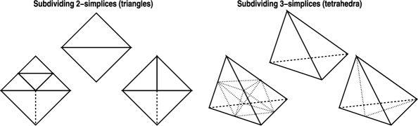
Figure 2. Refinement of 2- and 3-simplices using 4-section, 8-section, and bisection.

The paired triangle in the 2-simplex case of Figure 2 illustrates the nature of conformity and its violation during refinement. A globally conforming simplex mesh is defined as a collection of simplices which meet only at vertices and faces; for example, removing the dotted bisection in the third group from the left in Figure 2 produces a non-conforming mesh. Non-conforming simplex meshes create several theoretical as well as practical implementation difficulties; while the queue-swapping presented in Algorithm 2.2.1 above is a feature unique to MC (see Section 3), an equivalent approach is taken in PLTMG  [10] and similar packages [73, 25, 27, 24].

2.2.2. Computational complexity: solving linear and nonlinear systems

Addressing the complexity of Algorithm 2.2.1, Newton-like methods as illustrated in Algorithm 2.2.2 are often the most effective.

• (Damped-inexact-Newton)

  • Let an initial approximation $u$ be given.

  • While ($|\langle F(u),v\rangle|>\epsilon$ for any $v$) do:

    1. Find $w$ such that $\langle DF(u)w,v\rangle=-\langle F(u),v\rangle+r,~{}\forall~{}v$.

    2. Set $u=u+\lambda w$.

  • End While.

The bilinear form $\langle DF(u)w,v\rangle$ which appears in Algorithm 2.2.2 is simply the (Gateaux) linearization of the nonlinear form $\langle F(u),v\rangle$, defined formally as:

$$\langle DF(u)w,v\rangle=\left.\frac{d}{d\epsilon}\langle F(u+\epsilon w),v\rangle\right|_{\epsilon=0}.$$

This form is easily computed from most nonlinear forms $\langle F(u),v\rangle$ which arise from second order nonlinear elliptic problems, although the calculation can be tedious in some cases (the example we consider later in the paper is in this category). The possibly nonzero “residual” term $r$ is to allow for inexactness in the linearization solve for efficiency, which is quite effective in many cases (cf. [17, 40, 42]). The parameter $\lambda$ brings robustness to the algorithm [42, 15, 16]. If folds or bifurcations are present, then the iteration is modified to incorporate path-following [62, 14].

As was the case for the Petrov-Galerkin discretized nonlinear residual $\langle F(\cdot),\cdot\rangle$, the matrix representing the bilinear form in the Newton iteration is easily assembled, regardless of the complexity of the bilinear form $\langle DF(\cdot)\cdot,\cdot\rangle$. In particular, the matrix equation for $w=\sum_{j=1}^{n}\beta_{j}\phi_{j}$ has the form:

$$AU=F,\ \ \ \ \ U_{i}=\beta_{i},$$

where

$$A_{ij}=\langle DF(\bar{u}_{h}+\sum_{k=1}^{n}\alpha_{k}\phi_{k})\phi_{j},\psi_{i}\rangle,\ \ \ \ \ F_{i}=\langle F(\bar{u}_{h}+\sum_{j=1}^{n}\alpha_{j}\phi_{j}),\psi_{i}\rangle.$$

As long as the integral-based forms $\langle F(\cdot),\cdot\rangle$ and $\langle DF(\cdot)\cdot,\cdot\rangle$ can be evaluated at individual points in the domain, then quadrature can be used to build the Newton equations, regardless of the complexity of the forms. This is one of the most powerful features of the finite element method. It should be noted that there is a subtle difference between the approach outlined here (typical for a nonlinear finite element approximation) and that usually taken when applying a Newton-iteration to a nonlinear finite difference approximation. In particular, in the finite difference setting the discrete equations are linearized explicitly by computing the jacobian of the system of nonlinear algebraic equations. In the finite element setting, the commutativity of linearization and discretization is exploited; the Newton iteration is actually performed in function space, with discretization occurring “at the last moment” in Algorithm 2.2.2 above.

It can be shown that the Newton iteration above is dominated by the computational complexity of solving the $n$ linear algebraic equations in each iteration (cf. [17, 49]). Multilevel methods are the only known provably optimal or nearly optimal methods for solving these types of linear algebraic equations resulting from discretizations of a large class of general linear elliptic problems [49, 11, 94]. Unfortunately, the need to accurately represent complicated PDE coefficient, domain features, and domain boundaries with an adapted mesh requires the use of very fine mesh simply to describe the complexities of the problem, which often precludes the simple solve-estimate-refine approach in Algorithm 2.2.1. In Section 3.4 we describe the algebraic multilevel approach we take in the MC implementation to adress this, similar to that taken in [31, 32, 83, 89].

2.3. Residual-based a posteriori error indicators

There are several approaches to adaptive error control, although the approaches based on a posteriori error estimation are usually the most effective and most general. While most existing work on a posteriori estimates has been for linear problems, extensions to the nonlinear case can be made through linearization. For example, consider the nonlinear problem in (2.9), which we will write as follows (ignoring the parameters for simplicity):

$$F(u)=0,~{}~{}~{}F\in C^{1}({\mathcal{B}}_{1},{\mathcal{B}}_{2}^{*}),~{}~{}~{}{\mathcal{B}}_{1},{\mathcal{B}}_{2}~{}\text{Banach~{}spaces},$$ (2.35)

and a discretization:

$$F_{h}(u_{h})=0,~{}~{}~{}F_{h}\in C^{0}(U_{h},V_{h}^{*}),~{}~{}~{}U_{h}\subset{\mathcal{B}}_{1},~{}~{}~{}V_{h}\subset{\mathcal{B}}_{2}.$$ (2.36)

The nonlinear residual $F(u_{h})$ can be used to estimate the error $\|u-u_{h}\|_{{\mathcal{B}}_{1}}$, through the use of a linearization theorem [68, 90]. An example of such a theorem due to Verfürth is the following.

Theorem 2.1.

[90] Let $u\in X$ be a regular solution of $F(u)=0$, so that the Gateaux derivative $DF(u)$ is a linear homeomorphism of ${\mathcal{B}}_{1}$ onto ${\mathcal{B}}_{2}^{*}$. Assume $DF$ is Lipschitz continuous at $u$, so that there exists $R_{0}$ such that

$$\gamma=\sup_{u_{h}\in B(u,R_{0})}\frac{\|DF(u)-DF(u_{h})\|_{{\mathcal{L}}({\mathcal{B}}_{1},{\mathcal{B}}_{2}^{*})}}{\|u-u_{h}\|_{{\mathcal{B}}_{1}}}<\infty.$$

Let $R=\min\{R_{0},\gamma^{-1}\|DF(u)^{-1}\|_{{\mathcal{L}}({\mathcal{B}}_{2}^{*},{\mathcal{B}}_{1})},2\gamma^{-1}\|DF(u)\|_{{\mathcal{L}}({\mathcal{B}}_{1},{\mathcal{B}}_{2}^{*})}\}$. Then for all $u_{h}\in B(u,R)$,

$$C_{1}\|F(u_{h})\|_{{\mathcal{B}}_{2}^{*}}\leq\|u-u_{h}\|_{{\mathcal{B}}_{1}}\leq C_{2}\|F(u_{h})\|_{{\mathcal{B}}_{2}^{*}},$$ (2.37)

where $C_{1}=\frac{1}{2}\|DF(u)\|^{-1}_{{\mathcal{L}}({\mathcal{B}}_{1},{\mathcal{B}}_{2}^{*})}$ and $C_{2}=2\|DF(u)^{-1}\|_{{\mathcal{L}}({\mathcal{B}}_{2}^{*},{\mathcal{B}}_{1})}$.

Proof.

See [90].∎∎

The effect of linearization is swept under the rug somewhat by the choice of $R$ sufficiently small, where $R$ is the radius of an open ball in ${\mathcal{B}}_{1}$ about $u$, denoted as $B(u,R)$ in the theorem above. One then ignores the factors in (2.37) involving the linearization $DF(u)$ and its inverse, and focuses on two-sided estimates for the nonlinear residual $\|F(u_{h})\|_{{\mathcal{B}}_{2}^{*}}$ appearing on each side of (2.37). Since one typically constructs highly refined meshes where needed, such local linearized estimates are thought to reasonable, although much evidence to the contrary has been assembled by the dual-problem error indicator community (see the discussion later in this section). Note that $\|F(u_{h})\|_{{\mathcal{B}}_{2}^{*}}$ can be estimated in different ways, including

1. Approximation by $\|F_{h}(u_{h})\|_{{\mathcal{B}}_{2}^{*}}$ (residual estimates) [90, 91, 68, 69],

2. Solution of local Neumann (or Dirichlet) problems [18, 20].

The approaches can be shown to be essentially equivalent (up to constants; cf. [90, 23]). For reasons of efficiency, estimation by strong residuals is often used rather than the solution of local problems in the case of elliptic systems and/or in the setting of three-dimensional problems. In particular, one employs the linearization theorem above, together with some derived (and computable) upper and lower bounds on the nonlinear residual $\|F(u_{h})\|_{{\mathcal{B}}_{2}^{*}}$ given by the following pair of inequalities:

$$C_{3}\leq\|F(u_{h})\|_{{\mathcal{B}}_{2}^{*}}\leq C_{4}.$$

While it is clear that the upper bound $C_{4}$ is the key to bounding the error, the lower bound $C_{3}$ can also be quite useful; it can help to ensure that the adaptive procedure doesn’t do too much work by over-refining an area where it is unnecessary. The effectiveness of an adaptive finite element code can hinge on the implementation details of the estimator, and implementing it efficiently can be quite an art form (cf. [90, 18, 20]).

We now consider the first two of these approaches in more detail. First, we derive a strong residual-based a posteriori error indicator for general Petrov-Galerkin approximations (2.33) to the solutions of general nonlinear elliptic systems of tensors of the form (2.5)–(2.7). The analysis involves primarily the weak formulation (2.14)–(2.15). Our derivation follows closely that of Verfürth [90, 91] in the flat, Cartesian case. In the next section, we will consider the second alternative, namely an indicator based on a duality approach.

It should be noted that while the discussions throughout the paper are generally valid for domains which are connected compact Riemannian manifolds with Lipschitz continuous boundaries, several of the results we will need to employ here have only been shown to hold in the case of bounded $2$- and $3$-manifolds with smooth boundaries, with an atlas consisting of only one chart (i.e., bounded open subsets of ${\mathbb{R}}^{2}$ and ${\mathbb{R}}^{3}$). Examples are convex polyhedra in ${\mathbb{R}}^{d}$, which automatically satisfy the Lipschitz continuity assumption. The extensions of some of these results from open sets to Riemannian manifolds are not immediate; a number of subtle issues arise when manifold domains are considered in conjunction with Sobolev spaces, the subject of two recent monographs [4, 52]. Some of the difficulties encountered impact approximation theory on manifolds [1, 4, 82, 86, 52]. However, if a sufficient amount of the function space framework is in place, and if the underlying manifold admits a partition of unity (e.g., if it is paracompact), then it should be possible to extend finite element approximation theory by operating chartwise, and then globalizing the local results using the partition of unity. We will assume here that such extensions are possible; understanding the manifold case of multiple charts and other complications is work in progress [53].

The starting point for our residual-based error indicator is the linearization inequality (2.37). In our setting of the weak formulation (2.14)–(2.15), we make the appropriate choice (2.16)–(2.17), where we restrict our discussion here to a single elliptic system for a scalar or a $d$-vector (i.e., the product space has dimension $n_{e}=1$), which includes the examples presented later in the paper. The linearization inequality then involves standard Sobolev norms:

$$C_{1}\|F(u_{h})\|_{W^{-1,q}({\mathcal{M}})}\leq\|u-u_{h}\|_{W^{1,r}({\mathcal{M}})}\leq C_{2}\|F(u_{h})\|_{W^{-1,q}({\mathcal{M}})},$$ (2.38)

for $1/p+1/q=1$, $r\geq\text{min}\{p,q\}$, where $W^{-1,q}({\mathcal{M}})=(W^{1,q}({\mathcal{M}}))^{*}$ denotes the dual space of bounded linear functionals on $W^{1,q}({\mathcal{M}})$. The norm of the nonlinear residual $F(\cdot)$ in the dual space of bounded linear functionals on $W^{1,q}({\mathcal{M}})$ is defined in the usual way:

$$\|F(u)\|_{W^{-1,q}({\mathcal{M}})}=\sup_{0\neq v\in W^{1,q}({\mathcal{M}})}\frac{|\langle F(u),v\rangle|}{\|v\|_{W^{1,q}({\mathcal{M}})}}.$$ (2.39)

The numerator is the nonlinear weak form $\langle F(u),v\rangle$ appearing in (2.15). (We will consider only the case of no parameters; see [90] for the case of parameters.) In order to derive a bound on the weak form in the numerator we must first introduce quite a bit of notation that we have managed to avoid until now.

To begin, we assume that the $d$-manifold ${\mathcal{M}}$ has been exactly triangulated with a set ${\mathcal{S}}$ of shape-regular $d$-simplices (the finite dimension $d$ is arbitrary throughout this discussion). A family of simplices will be referred to here as shape-regular if for all simplices in the family the ratio of the diameter of the circumscribing sphere to that of the inscribing sphere is bounded by an absolute fixed constant, independent of the numbers and sizes of the simplices that may be generated through refinements. (For a more careful definition of shape-regularity and related concepts, see [35].) It will be convenient to introduce the following notation:

${\mathcal{S}}$	=	Set of shape-regular simplices triangulating ${\mathcal{M}}$
${\mathcal{N}}(s)$	=	Union of faces in simplex set $s$ lying on $\partial_{N}{\mathcal{M}}$
${\mathcal{I}}(s)$	=	Union of faces in simplex set $s$ not in ${\mathcal{N}}(s)$
${\mathcal{F}}(s)$	=	${\mathcal{N}}(s)\cup{\mathcal{I}}(s)$
$\omega_{s}$	=	$~{}\bigcup~{}\{~{}\tilde{s}\in{\mathcal{S}}~{}|~{}s\bigcap\tilde{s}\neq\emptyset,~{}\text{where}~{}s\in{\mathcal{S}}~{}\}$
$\omega_{f}$	=	$~{}\bigcup~{}\{~{}\tilde{s}\in{\mathcal{S}}~{}|~{}f\bigcap\tilde{s}\neq\emptyset,~{}\text{where}~{}f\in{\mathcal{F}}~{}\}$
$h_{s}$	=	Diameter (inscribing sphere) of the simplex $s$
$h_{f}$	=	Diameter (inscribing sphere) of the face $f$.

When the argument to one of the face set functions ${\mathcal{N}}$, ${\mathcal{I}}$, or ${\mathcal{F}}$ is in fact the entire set of simplices ${\mathcal{S}}$, we will leave off the explicit dependence on ${\mathcal{S}}$ without danger of confusion. Referring forward briefly to Figure 3 will be convenient. The two darkened triangles in the left picture in Figure 3 represents the set $w_{f}$ for the face $f$ shared by the two triangles. The clear triangles in the right picture in Figure 3 represents the set $w_{s}$ for the darkened triangle $s$ in the center (the set $w_{s}$ also includes the darkened triangle).

Finally, we will also need some notation to represent discontinuous jumps in function values across faces interior to the triangulation. To begin, for any face $f\in{\mathcal{N}}$, let $n_{f}$ denote the unit outward normal; for any face $f\in{\mathcal{I}}$, take $n_{f}$ to be an arbitrary (but fixed) choice of one of the two possible face normal orientations. Now, for any $v\in L^{2}({\mathcal{M}})$ such that $v\in C^{0}(s)~{}\forall s\in{\mathcal{S}}$, define the jump function:

$$[v]_{f}(x)=\lim_{\epsilon\rightarrow 0^{+}}v(x+\epsilon n_{f})-\lim_{\epsilon\rightarrow 0^{-}}v(x-\epsilon n_{f}).$$

We now begin the analysis by splitting the volume and surface integrals in (2.15) into sums of integrals over the individual elements and faces, and we then employ the divergence theorem (2.1) to work backward towards the strong form in each element:

$$\langle F(u),v\rangle = \int_{{\mathcal{M}}}{\mathcal{G}}_{ij}(A^{ia}v^{j}_{~{};a}+B^{i}v^{j})~{}dx+\int_{\partial_{N}{\mathcal{M}}}{\mathcal{G}}_{ij}C^{i}v^{j}~{}ds$$

$$= \sum_{s\in{\mathcal{S}}}\int_{s}{\mathcal{G}}_{ij}(A^{ia}v^{j}_{~{};a}+B^{i}v^{j})~{}dx+\sum_{f\in{\mathcal{N}}}\int_{f}{\mathcal{G}}_{ij}C^{i}v^{j}~{}ds$$

$$= \sum_{s\in{\mathcal{S}}}\int_{s}{\mathcal{G}}_{ij}(B^{i}-A^{ia}_{~{}~{};a})v^{j}~{}dx+\sum_{s\in{\mathcal{S}}}\int_{\partial s}{\mathcal{G}}_{ij}A^{ia}n_{a}v^{j}~{}ds$$

$$\quad+\sum_{f\in{\mathcal{N}}}\int_{f}{\mathcal{G}}_{ij}C^{i}v^{j}~{}ds.$$

Using the fact that (2.33) holds for the solution to the discrete problem, we employ the jump function and write

$$\langle F(u_{h}),v\rangle = \langle F(u_{h}),v-v_{h}\rangle$$

$$= \sum_{s\in{\mathcal{S}}}\int_{s}{\mathcal{G}}_{ij}(B^{i}-A^{ia}_{~{}~{};a})(v^{j}-v^{j}_{h})~{}dx$$

$$+\sum_{s\in{\mathcal{S}}}\int_{\partial s}{\mathcal{G}}_{ij}A^{ia}n_{a}(v^{j}-v^{j}_{h})~{}ds$$

$$+\sum_{f\in{\mathcal{N}}}\int_{f}{\mathcal{G}}_{ij}C^{i}(v^{j}-v^{j}_{h})~{}ds$$

$$= \sum_{s\in{\mathcal{S}}}\int_{s}{\mathcal{G}}_{ij}(B^{i}-A^{ia}_{~{}~{};a})(v^{j}-v^{j}_{h})~{}dx$$

$$+\sum_{f\in{\mathcal{I}}}\int_{f}{\mathcal{G}}_{ij}\left[A^{ia}n_{a}\right]_{f}(v^{j}-v^{j}_{h})~{}ds$$

$$\quad+\sum_{f\in{\mathcal{N}}}\int_{f}{\mathcal{G}}_{ij}(C^{i}+A^{ia}n_{a})(v^{j}-v^{j}_{h})~{}ds$$

$$\leq \sum_{s\in{\mathcal{S}}}\left(\|B^{i}-A^{ia}_{~{}~{};a}\|_{L^{p}(s)}\|v^{j}-v^{j}_{h}\|_{L^{q}(s)}\right)$$

$$+\sum_{f\in{\mathcal{I}}}\left(\|\left[A^{ia}n_{a}\right]_{f}\|_{L^{p}(f)}\|v^{j}-v^{j}_{h}\|_{L^{q}(f)}\right)$$

$$\quad+\sum_{f\in{\mathcal{N}}}\left(\|C^{i}+A^{ia}n_{a}\|_{L^{p}(f)}\|v^{j}-v^{j}_{h}\|_{L^{q}(f)}\right),$$

where we have applied the Hölder inequality (2.23) three times with $1/p+1/q=1$.

In order to bound the sums on the right, we will employ a standard tool known as a $W^{1,p}$-quasi-interpolant $I_{h}$. An example of such an interpolant is due to Scott and Zhang [87], which we refer to as the SZ-interpolant (see also Clément’s interpolant in [36]). Unlike point-wise polynomial interpolation, which is not well-defined for functions in $W^{1,p}({\mathcal{M}})$ when the embedding $W^{1,p}({\mathcal{M}})\hookrightarrow C^{0}({\mathcal{M}})$ fails, the SZ-interpolant $I_{h}$ can be constructed quite generally for $W^{1,p}$-functions on shape-regular meshes of $2$- and $3$-simplices. Moreover, it can be shown to have the following remarkable local approximation properties: For all $v\in W^{1,q}({\mathcal{M}})$, it holds that

$$\|v-I_{h}v\|_{L^{q}(s)} \leq C_{s}h_{s}\|v\|_{W^{1,q}(\omega_{s})},$$ (2.41)

$$\|v-I_{h}v\|_{L^{q}(f)} \leq C_{f}h_{f}^{1-1/q}\|v\|_{W^{1,q}(\omega_{f})}.$$ (2.42)

For the construction of the SZ-interpolant, and for a proof of the approximation inequalities in $L^{p}$-spaces for $p\neq 2$, see [87]. A simple construction and the proof of the first inequality can also be found in the appendix of [57].

Employing now the SZ-interpolant by taking $v_{h}=I_{h}v$ in (2.3), using (2.41)–(2.42), and noting that $1-1/q=1/p$, we have

$$\langle F(u_{h}),v\rangle \leq \sum_{s\in{\mathcal{S}}}C_{s}h_{s}\|B^{i}-A^{ia}_{~{}~{};a}\|_{L^{p}(s)}\|v^{j}\|_{W^{1,q}(\omega_{s})}$$

$$+\sum_{f\in{\mathcal{I}}}C_{f}h_{f}^{1/p}\|\left[A^{ia}n_{a}\right]_{f}\|_{L^{p}(f)}\|v^{j}\|_{W^{1,q}(\omega_{f})}$$

$$+\sum_{f\in{\mathcal{N}}}C_{f}h_{f}^{1/p}\|C^{i}+A^{ia}n_{a}\|_{L^{p}(f)}\|v^{j}\|_{W^{1,q}(\omega_{f})}$$

$$\leq \left(\sum_{s\in{\mathcal{S}}}C_{s}^{p}h_{s}^{p}\|B^{i}-A^{ia}_{~{}~{};a}\|_{L^{p}(s)}^{p}\right.$$

$$\left.+\sum_{f\in{\mathcal{I}}}C_{f}^{p}h_{f}\|\left[A^{ia}n_{a}\right]_{f}\|_{L^{p}(f)}^{p}+\sum_{f\in{\mathcal{N}}}C_{f}^{p}h_{f}\|C^{i}+A^{ia}n_{a}\|_{L^{p}(f)}^{p}\right)^{1/p}$$

$$\cdot\left(\sum_{s\in{\mathcal{S}}}\|v^{j}\|_{W^{1,q}(\omega_{s})}^{q}+\sum_{f\in{\mathcal{I}}}\|v^{j}\|_{W^{1,q}(\omega_{f})}^{q}+\sum_{f\in{\mathcal{N}}}\|v^{j}\|_{W^{1,q}(\omega_{f})}^{q}\right)^{1/q}$$

where we have used the discrete Hölder inequality to obtain the last inequality.

It is not difficult to show (cf. [90]) that the simplex shape regularity assumption bounds the number of possible overlaps of the sets $\omega_{s}$ with each other, and also bounds the number of possible overlaps of the sets $\omega_{f}$ with each other. This makes it possible to establish the following two inequalities:

$$\sum_{s\in{\mathcal{S}}}\|v^{j}\|_{W^{1,q}(\omega_{s})}^{q} \leq D_{s}\|v\|_{W^{1,q}({\mathcal{M}})}^{q},$$ (2.44)

$$\sum_{f\in{\mathcal{F}}}\|v^{j}\|_{W^{1,q}(\omega_{f})}^{q} \leq D_{f}\|v\|_{W^{1,q}({\mathcal{M}})}^{q},$$ (2.45)

where $D_{s}$ and $D_{f}$ depend on the shape regularity constants reflecting these overlap bounds. Therefore, since ${\mathcal{I}}\subset{\mathcal{F}}$ and ${\mathcal{N}}\subset{\mathcal{F}}$, we employ (2.44)–(2.45) in (2.3) which gives

$$\langle F(u_{h}),v\rangle \leq C_{5}\|v\|_{W^{1,q}({\mathcal{M}})}\cdot\left(\sum_{s\in{\mathcal{S}}}h_{s}^{p}\|B^{i}-A^{ia}_{~{}~{};a}\|_{L^{p}(s)}^{p}\right.$$

$$+ \sum_{f\in{\mathcal{I}}}h_{f}\|\left[A^{ia}n_{a}\right]_{f}\|_{L^{p}(f)}^{p}\left.+\sum_{f\in{\mathcal{N}}}h_{f}\|C^{i}+A^{ia}n_{a}\|_{L^{p}(f)}^{p}\right)^{1/p},$$

where $C_{5}=\max_{{\mathcal{S}},{\mathcal{F}}}\{C_{s},C_{f}\}\cdot\max_{{\mathcal{S}},{\mathcal{F}}}\{D_{s}^{1/q},D_{f}^{1/q}\}$ depends on the shape regularity of the simplices in ${\mathcal{S}}$.

We finally now use (2.3) in (2.39) to achieve the upper bound in (2.38):

$$\|u-u_{h}\|_{W^{1,r}({\mathcal{M}})} \leq C_{2}\|F(u_{h})\|_{W^{-1,q}({\mathcal{M}})}$$

$$= C_{2}\sup_{0\neq v\in W^{1,q}({\mathcal{M}})}\frac{|\langle F(u_{h}),v\rangle|}{\|v\|_{W^{1,q}({\mathcal{M}})}}$$

$$\leq C_{2}C_{5}\left(\sum_{s\in{\mathcal{S}}}h_{s}^{p}\|B^{i}-A^{ia}_{~{}~{};a}\|_{L^{p}(s)}^{p}\right.$$

$$+\sum_{f\in{\mathcal{I}}}h_{f}\|\left[A^{ia}n_{a}\right]_{f}\|_{L^{p}(f)}^{p}$$

$$\left.+\sum_{f\in{\mathcal{N}}}h_{f}\|C^{i}+A^{ia}n_{a}\|_{L^{p}(f)}^{p}\right)^{1/p}.$$

We will make one final transformation that will turn this into a sum of element-wise error indicators that will be easier to work with in an implementation. We only need to account for the interior face integrals (which would otherwise be counted twice) when we combine the sum over the faces into the sum over the elements. This leave us with the following

Theorem 2.2.

Let $u\in W^{1,r}({\mathcal{M}})$ be a regular solution of (2.5)–(2.7), or equivalently of (2.14)–(2.15), where (2.16)–(2.17) holds. Then under the same assumptions as in Theorem 2.1, the following a posteriori error estimate holds for a Petrov-Galerkin approximation $u_{h}$ satisfying (2.33):

$$\|u-u_{h}\|_{W^{1,r}({\mathcal{M}})}\leq C\left(\sum_{s\in{\mathcal{S}}}\eta_{s}^{p}\right)^{1/p},$$ (2.48)

where

$$C=2\cdot\max_{{\mathcal{S}},{\mathcal{F}}}\{C_{s},C_{f}\}\cdot\max_{{\mathcal{S}},{\mathcal{F}}}\{D_{s}^{1/q},D_{f}^{1/q}\}\cdot\|DF(u)^{-1}\|_{{\mathcal{L}}(W^{-1,q},W^{1,p})},$$

and where the element-wise error indicator $\eta_{s}$ is defined as:

$$\eta_{s} = \left(h_{s}^{p}\|B^{i}-A^{ia}_{~{}~{};a}\|_{L^{p}(s)}^{p}+\frac{1}{2}\sum_{f\in{\mathcal{I}}(s)}h_{f}\|\left[A^{ia}n_{a}\right]_{f}\|_{L^{p}(f)}^{p}\right.$$

$$\left.+\sum_{f\in{\mathcal{N}}(s)}h_{f}\|C^{i}+A^{ia}n_{a}\|_{L^{p}(f)}^{p}\right)^{1/p}.$$

Proof.

The proof follows from (2.3) and the discussion above.∎∎

The element-wise error indicator in (2.2) provides an error bound in the $W^{1,r}$-norm for a general covariant nonlinear elliptic system of the form (2.5)–(2.7), with $1/p+1/q=1$, $r\geq\text{min}\{p,q\}$, which may be more appropriate than the $r=p=q=2$ case for some nonlinear problems. Issues related to this topic are discussed in [90]. Following [90], it is possible to use a similar analysis to construct lower bounds, dual to (2.48), of the form

$$\tilde{C}\left(\sum_{s\in{\mathcal{S}}}\eta_{s}^{p}\right)^{1/p}\leq\|u-u_{h}\|_{W^{1,r}({\mathcal{M}})}.$$

Such results are useful for performing unrefinement and in accessing the quality of an error-indicator.

2.4. Duality-based a posteriori error indicators

We now derive an alternative a posteriori error indicator for general Petrov-Galerkin approximations (2.33) to the solutions of general nonlinear elliptic systems of tensors of the form (2.5)–(2.7). The indicator is based on the solution of a global linearized adjoint (or dual) problem; again the analysis involves primarily the weak formulation (2.14)–(2.15), and follows closely that of [23, 43]. This approach can be viewed as simply another way to bound the nonlinear residual $\|F(u_{h})\|_{{\mathcal{B}}_{2}^{*}}$ after employing the (possibly quite crude) one-time linearization in Theorem 2.1. However, the approach can be used to avoid the one-time linearization step, bringing the stability properties of the differential operator into the error indicator by updating the linearization as the solution is improved, and by incorporating the linearization operator itself into the error indicator.

As before, we are interested in the solution to the operator equation (2.35) and also in error estimates for approximations $u_{h}$ satisfying (2.36). We begin with the generalized Taylor remainder in integral form:

$$F(u+h)=F(u)+\left\{\int_{0}^{1}DF(u+\xi h)d\xi\right\}h.$$ (2.50)

Taking $h=u_{h}-u$, the error $e=u-u_{h}$ can be expressed as follows:

$$R=-F(u_{h})=-F(u+[u_{h}-u])=-F(u)-A(u_{h}-u)=0-Ae,$$

where the linearization operator $A$ is defined from (2.50) as:

$$A=\int_{0}^{1}DF(u+\xi h)d\xi.$$ (2.51)

If a linear functional of the error $l(e)=\langle e,\psi\rangle$ is of interest rather than the error itself, where $\psi$ is the Riesz-representer of $l(\cdot)$, then we can exploit the linearization operator $A$ in (2.51), and its (unique) adjoint $A^{T}$, to produce an error indicator:

$$|\langle e,\psi\rangle|=|\langle e,A^{T}\phi\rangle|=|\langle Ae,\phi\rangle|=|\langle R,\phi\rangle|=|\langle F(u_{h}),\phi\rangle|.$$

The indicator requires the solution of the linearized dual problem:

$$A^{T}\phi=\psi$$ (2.52)

for the residual weights $\phi$, where the data for the dual problem $\psi$ is the Riesz-representer of the functional of interest. Strong norm estimates of the form (2.38) can be established using duality (cf. [23]), but the operator information represented by the dual solution $\phi$ is then lost (it appears in the constants). If a functional of the error is of interest (e.g., the error along a curve or surface in the domain), then a more delicate approach is to instead employ the dual solution $\phi$ as part of the indicator:

$$|\langle e,\psi\rangle|=|\langle F(u_{h}),\phi\rangle|\leq error~{}estimate.$$ (2.53)

The dual solution $\phi$ obtained by solving (2.52) is used locally (element-wise) in (2.53), with the dual solution as residual weights (cf. [43]).

To construct such estimates for general Petrov-Galerkin approximations (2.33) to the solutions of general nonlinear elliptic systems of tensors of the form (2.5)–(2.7), we first need some simple identities to help identify the form of the linearized dual problem:

$$A^{ia}(u^{k},u^{k}_{~{};c})-A^{ia}(U^{k},U^{k}_{~{};c})~{}~{}~{}~{}~{}~{}~{}~{}~{}~{}~{}~{}~{}~{}~{}~{}~{}~{}~{}~{}~{}~{}~{}~{}~{}~{}~{}~{}~{}~{}~{}~{}~{}~{}~{}~{}~{}~{}~{}~{}~{}~{}~{}~{}~{}~{}~{}~{}~{}~{}~{}~{}~{}~{}~{}~{}~{}~{}~{}~{}~{}~{}~{}~{}~{}~{}~{}~{}$$

$$= \int_{0}^{1}\frac{d}{ds}A^{ia}(su^{k}+(1-s)U^{k},su^{k}_{~{};c}+(1-s)U^{k}_{~{};c})ds$$

$$= \int_{0}^{1}\left\{D_{1}A^{ia}(su^{k}+(1-s)U^{k},su^{k}_{~{};c}+(1-s)U^{k}_{~{};c})\right.$$

$$~{}~{}~{}~{}\cdot\frac{d}{ds}[su^{k}+(1-s)U^{k}]$$

$$+D_{2}A^{ia}(su^{k}+(1-s)U^{k},su^{k}_{~{};c}+(1-s)U^{k}_{~{};c})$$

$$~{}~{}~{}~{}\cdot\left.\frac{d}{ds}[su^{k}_{~{};c}+(1-s)U^{k}_{~{};c}]\right\}ds$$

$$= \left\{\int_{0}^{1}D_{1}A^{ia}(su^{k}+(1-s)U^{k},su^{k}_{~{};c}+(1-s)U^{k}_{~{};c})ds\right\}(u^{k}-U^{k})$$

$$+\left\{\int_{0}^{1}D_{2}A^{ia}(su^{k}+(1-s)U^{k},su^{k}_{~{};c}+(1-s)U^{k}_{~{};c})ds\right\}(u^{k}_{;c}-U^{k}_{;c})$$

$$= {\mathcal{A}}^{ia}_{~{}~{}b}e^{b}+{\mathcal{A}}^{ia~{}c}_{~{}~{}b}e^{b}_{~{};c}.$$

$$B^{i}(u^{k},u^{k}_{~{};c})-B^{i}(U^{k},U^{k}_{~{};c})~{}~{}~{}~{}~{}~{}~{}~{}~{}~{}~{}~{}~{}~{}~{}~{}~{}~{}~{}~{}~{}~{}~{}~{}~{}~{}~{}~{}~{}~{}~{}~{}~{}~{}~{}~{}~{}~{}~{}~{}~{}~{}~{}~{}~{}~{}~{}~{}~{}~{}~{}~{}~{}~{}~{}~{}~{}~{}~{}~{}~{}~{}~{}~{}~{}~{}~{}~{}$$

$$= \int_{0}^{1}\frac{d}{ds}B^{i}(su^{k}+(1-s)U^{k},su^{k}_{~{};c}+(1-s)U^{k}_{~{};c})ds$$

$$= \int_{0}^{1}\left\{D_{1}B^{i}(su^{k}+(1-s)U^{k},su^{k}_{~{};c}+(1-s)U^{k}_{~{};c})\right.$$

$$~{}~{}~{}~{}\cdot\frac{d}{ds}[su^{k}+(1-s)U^{k}]$$

$$+D_{2}B^{i}(su^{k}+(1-s)U^{k},su^{k}_{~{};c}+(1-s)U^{k}_{~{};c})$$

$$~{}~{}~{}~{}\cdot\left.\frac{d}{ds}[su^{k}_{~{};c}+(1-s)U^{k}_{~{};c}]\right\}ds$$

$$= \left\{\int_{0}^{1}D_{1}B^{i}(su^{k}+(1-s)U^{k},su^{k}_{~{};c}+(1-s)U^{k}_{~{};c})ds\right\}(u^{k}-U^{k})$$

$$+\left\{\int_{0}^{1}D_{2}B^{i}(su^{k}+(1-s)U^{k},su^{k}_{~{};c}+(1-s)U^{k}_{~{};c})ds\right\}(u^{k}_{;c}-U^{k}_{;c})$$

$$= {\mathcal{B}}^{i}_{~{}b}e^{b}+{\mathcal{B}}^{i~{}c}_{~{}b}e^{b}_{~{};c}.$$

Similarly,

$$C^{i}(u^{k})-C^{i}(U^{k})=\left\{\int_{0}^{1}D_{1}C^{i}(su^{k}+(1-s)U^{k})ds\right\}(u^{k}-U^{k})={\mathcal{C}}^{i}_{~{}b}e^{b}.$$

Therefore, given our original weak form in (2.15), we have

$$\langle F(u)-F(U),\phi\rangle = \int_{{\mathcal{M}}}{\mathcal{G}}_{ij}\left\{[A^{ia}(u^{k},u^{k}_{~{};c})-[A^{ia}(U^{k},U^{k}_{~{};c})]\phi^{j}_{~{};a}\right.$$

$$\left.+~{}[B^{i}(u^{k},u^{k}_{~{};c})-B^{i}(U^{k},U^{k}_{~{};c})]\phi^{j}\right\}~{}dx$$

$$+\int_{\partial_{1}{\mathcal{M}}}{\mathcal{G}}_{ij}[C^{i}(u^{k})-C^{i}(U^{k})]\phi^{j}~{}ds$$

$$= \int_{{\mathcal{M}}}{\mathcal{G}}_{ij}\left\{({\mathcal{A}}^{ia}_{~{}~{}b}e^{b}+{\mathcal{A}}^{ia~{}c}_{~{}~{}b}e^{b}_{~{};c})\phi^{j}_{~{};a}\right.$$

$$\left.+~{}({\mathcal{B}}^{i}_{~{}b}e^{b}+{\mathcal{B}}^{i~{}c}_{~{}b}e^{b}_{~{};c})\phi^{j}\right\}~{}dx+\int_{\partial_{1}{\mathcal{M}}}{\mathcal{G}}_{ij}{\mathcal{C}}^{i}_{~{}b}e^{b}\phi^{j}~{}ds$$

$$= \langle Ae,\phi\rangle$$

$$= \langle e,A^{T}\phi\rangle.$$

The weak form of the linearized dual problem is then:

$$\text{Find}~{}\phi\in{\mathcal{B}}_{1}~{}\text{such~{}that}~{}\langle A^{T}\phi,v\rangle=\langle\psi,v\rangle,~{}~{}~{}~{}\forall v\in{\mathcal{B}}_{2},$$ (2.54)

where the adjoint form is

$$\langle A^{T}\phi,v\rangle=\int_{{\mathcal{M}}}{\mathcal{G}}_{ij}\left\{{\mathcal{A}}^{ia~{}c}_{~{}~{}b}\phi^{j}_{~{};a}v^{b}_{~{};c}+{\mathcal{A}}^{ia}_{~{}~{}b}\phi^{j}_{~{};a}v^{b}+{\mathcal{B}}^{i~{}c}_{~{}b}\phi^{j}v^{b}_{~{};c}\right.$$ (2.55)

$$\left.+~{}{\mathcal{B}}^{i}_{~{}b}\phi^{j}v^{b}\right\}~{}dx+\int_{\partial_{1}{\mathcal{M}}}{\mathcal{G}}_{ij}{\mathcal{C}}^{i}_{~{}b}\phi^{j}v^{b}~{}ds.$$

The strong form of the linearized dual problem in (2.54)–(2.55) is then:

$${\mathcal{G}}_{ij}\left\{{\mathcal{A}}^{ia}_{~{}~{}b}\phi^{j}_{~{};a}-\left({\mathcal{A}}^{ia~{}c}_{~{}~{}b}\phi^{j}_{~{};a}\right)_{;c}+{\mathcal{B}}^{i}_{~{}b}\phi^{j}-\left({\mathcal{B}}^{i~{}c}_{~{}b}\phi^{j}\right)_{;c}\right\} = 0\text{~{}in~{}}{\mathcal{M}},$$

$${\mathcal{G}}_{ij}\left\{{\mathcal{A}}^{ia~{}c}_{~{}~{}b}\phi^{j}_{~{};a}n_{c}+\left({\mathcal{B}}^{i~{}c}_{~{}b}n_{c}+{\mathcal{C}}^{i}_{~{}b}\right)\phi^{j}\right\} = 0\text{~{}on~{}}\partial_{1}{\mathcal{M}},$$

$$u^{i}(x^{b}) = 0\text{~{}on~{}}\partial_{0}{\mathcal{M}}.$$

This leads to the following error representation:

Theorem 2.3.

Given a projector $P_{h}:{\mathcal{B}}_{1}\mapsto U_{h}$ onto the finite element subspace $U_{h}\subset{\mathcal{B}}_{1}$, the functional error is:

$$\langle e,\psi\rangle=\langle{\mathcal{R}}(U),\phi\rangle,$$

where

$$\langle{\mathcal{R}}(U),v\rangle = \sum_{s\in{\mathcal{S}}}\int_{s}{\mathcal{G}}_{ij}(B^{i}-A^{ia}_{~{}~{};a})(v^{j}-P_{h}v^{j})~{}dx$$

$$+\sum_{f\in{\mathcal{I}}}\int_{f}{\mathcal{G}}_{ij}\left[A^{ia}n_{a}\right]_{f}(v^{j}-P_{h}v^{j})~{}ds$$

$$+\sum_{f\in{\mathcal{N}}}\int_{f}{\mathcal{G}}_{ij}(C^{i}+A^{ia}n_{a})(v^{j}-P_{h}v^{j})~{}ds.$$

Proof.

We begin by working backward toward the strong form:

$$\langle e,\psi\rangle = \langle F(U),\phi\rangle$$

$$= \int_{{\mathcal{M}}}{\mathcal{G}}_{ij}(A^{ia}\phi^{j}_{~{};a}+B^{i}\phi^{j})~{}dx+\int_{\partial_{N}{\mathcal{M}}}{\mathcal{G}}_{ij}C^{i}\phi^{j}~{}ds$$

$$= \sum_{s\in{\mathcal{S}}}\int_{s}{\mathcal{G}}_{ij}(A^{ia}\phi^{j}_{~{};a}+B^{i}\phi^{j})~{}dx+\sum_{f\in{\mathcal{N}}}\int_{f}{\mathcal{G}}_{ij}C^{i}\phi^{j}~{}ds$$

$$= \sum_{s\in{\mathcal{S}}}\int_{s}{\mathcal{G}}_{ij}(B^{i}-A^{ia}_{~{}~{};a})\phi^{j}~{}dx+\sum_{s\in{\mathcal{S}}}\int_{\partial s}{\mathcal{G}}_{ij}A^{ia}n_{a}\phi^{j}~{}ds$$

$$+\sum_{f\in{\mathcal{N}}}\int_{f}{\mathcal{G}}_{ij}C^{i}\phi^{j}~{}ds.$$

Using then Galerkin orthogonality and a jump function gives:

$$\langle F(U),\phi\rangle = \langle F(U),\phi-P_{h}\phi\rangle$$

$$= \sum_{s\in{\mathcal{S}}}\int_{s}{\mathcal{G}}_{ij}(B^{i}-A^{ia}_{~{}~{};a})(\phi^{j}-P_{h}\phi^{j})~{}dx$$

$$+\sum_{s\in{\mathcal{S}}}\int_{\partial s}{\mathcal{G}}_{ij}A^{ia}n_{a}(\phi^{j}-P_{h}\phi^{j})~{}ds$$

$$+\sum_{f\in{\mathcal{N}}}\int_{f}{\mathcal{G}}_{ij}C^{i}(\phi^{j}-P_{h}\phi^{j})~{}ds$$

$$= \sum_{s\in{\mathcal{S}}}\int_{s}{\mathcal{G}}_{ij}(B^{i}-A^{ia}_{~{}~{};a})(\phi^{j}-P_{h}\phi^{j})~{}dx$$

$$+\sum_{f\in{\mathcal{I}}}\int_{f}{\mathcal{G}}_{ij}\left[A^{ia}n_{a}\right]_{f}(\phi^{j}-P_{h}\phi^{j})~{}ds$$

$$+\sum_{f\in{\mathcal{N}}}\int_{f}{\mathcal{G}}_{ij}(C^{i}+A^{ia}n_{a})(\phi^{j}-P_{h}\phi^{j})~{}ds$$

$$= \langle{\mathcal{R}}(U),\phi\rangle.$$

∎ ∎

The error representation can be used as an error indicator as illustrated in Algorithm 2.4.

• (Linearized dual error indicator)

  1. Decide which linear functional(s) of the error $l(e)=\langle e,\psi\rangle$ is of interest.

  2. Pose and solve the linearized dual problem $A^{T}\phi=\psi$ for the dual weight function $\phi$.

  3. Numerically approximate $\langle{\mathcal{R}}(U),\phi\rangle$ within each element as an element-wise error indicator.

  4. Elements which fail an indicator test (using equi-distribution) are marked for refinement.

3. Manifold Code (MC): adaptive multilevel finite element methods on manifolds

MC(see also [54, 8, 9, 55, 26]) is an adaptive multilevel finite element software package, written in ANSI C, which was developed by the author over several years at Caltech and UC San Diego. It is designed to produce highly accurate numerical solutions to nonlinear covariant elliptic systems of tensor equations on 2- and 3-manifolds in an optimal or nearly-optimal way. MC employs a posteriori error estimation, adaptive simplex subdivision, unstructured algebraic multilevel methods, global inexact Newton methods, and numerical continuation methods for the highly accurate numerical solution of nonlinear covariant elliptic systems on (Riemannian) 2- and 3-manifolds.

3.1. The overall design of MC

MC is an implementation of Algorithm 2.2.1, where Algorithm 2.2.2 is employed for solving nonlinear elliptic systems that arise in Step 1 of Algorithm 2.2.1. The linear Newton equations in each iteration of Algorithm 2.2.2 are solved with algebraic multilevel methods, and the algorithm is supplemented with a continuation technique when necessary. Several of the features of MC are somewhat unusual, allowing for the treatment of very general nonlinear elliptic systems of tensor equations on domains with the structure of 2- and 3-manifolds. In particular, some of these features are:

• Abstraction of the elliptic system: The elliptic system is defined only through a nonlinear weak form over the domain manifold, along with an associated linearization form, also defined everywhere on the domain manifold (precisely the forms $\langle F(u),v\rangle$ and $\langle DF(u)w,v\rangle$ in the discussions above). To use the a posteriori error indicators, a third function $F(u)$ must also be provided (essentially the strong form of the problem).

• Abstraction of the domain manifold: The domain manifold is specified by giving a polyhedral representation of the topology, along with an abstract set of coordinate labels of the user’s interpretation, possibly consisting of multiple charts. MC works only with the topology of the domain, the connectivity of the polyhedral representation. The geometry of the domain manifold is provided only through the form definitions, which contain the manifold metric information, and through a oneChart() routine that the user provides to resolve chart boundaries.

• Dimension independence: Exactly the same code paths in MC are taken for both two- and three-dimensional problems (as well as for higher-dimensional problems). To achieve this dimension independence, MC employs the simplex as its fundamental geometrical object for defining finite element bases.

As a consequence of the abstract weak form approach to defining the problem, the complete definition of a complex nonlinear tensor system such as large deformation nonlinear elasticity requires writing only a few hundred lines of C to define the two weak forms, and to define the oneChart() routine. Changing to a different tensor system (e.g. the example later in the paper involving the constraints in the Einstein equations) involves providing only a different definition of the forms and a different domain description.

3.2. Topology and geometry representation in MC: The Ringed Vertex

A datastructure referred to as the ringed-vertex (cf. [53]) is used to represent meshes of $d$-simplices of arbitrary topology. This datastructure is illustrated in Figure 3.

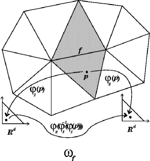
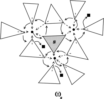
Figure 3. Polyhedral manifold representation. The figure on the left shows two overlapping polyhedral (vertex) charts consisting of the two rings of simplices around two vertices sharing an edge. The region consisting of the two darkened triangles around the face $f$ is denoted $\omega_{f}$, and represents the overlap of the two vertex charts. Polyhedral manifold topology is represented by MC using the ringed-vertex (or RIVER) datastructure. The datastructure is illustrated for a given simplex $s$ in the figure on the right; the topology primitives are vertices and $d$-simplices. The collection of the simplices which meet the simplex $s$ at its vertices (which then includes those simplices that share faces as well) is denoted as $\omega_{s}$. (The set $\omega_{s}$ includes $s$ itself.) Edges are temporarily created during subdivision but are then destroyed (a similar ring datastructure is used to represent the edge topology).

The ringed-vertex datastructure is similar to the winged-edge, quad-edge, and edge-facet datastructures commonly used in the computational geometry community for representing 2-manifolds [72], but it can be used more generally to represent arbitrary $d$-manifolds, $d\geq 2$. It maintains a mesh of $d$-simplices with near minimal storage, yet for shape-regular (non-degenerate) meshes, it provides $O(1)$-time access to all information necessary for refinement, un-refinement, and Petrov-Galerkin discretization of a differential operator. The ringed-vertex datastructure also allows for dimension independent implementations of mesh refinement and mesh manipulation, with one implementation (the same code path) covering arbitrary dimension $d$. An interesting feature of this datastructure is that the C structures used for vertices, simplices, and edges are all of fixed size, so that a fast array-based implementation is possible, as opposed to a less-efficient list-based approach commonly taken for finite element implementations on unstructured meshes. A detailed description of the ringed-vertex datastructure, along with a complexity analysis of various traversal algorithms, can be found in [53].

Since MC is based entirely on the $d$-simplex, for adaptive refinement it employs simplex bisection, using one of the simplex bisection strategies outlined earlier. Bisection is first used to refine an initial subset of the simplices in the mesh (selected according to some error indicator combined with equi-distribution, discussed below), and then a closure algorithm is performed in which bisection is used recursively on any non-conforming simplices, until a conforming mesh is obtained. If it is necessary to improve element shape, MC attempts to optimize the following simplex shape measure function for a given $d$-simplex $s$, in an iterative fashion, similar to the approach taken in [19]:

$$\eta(s,d)=\frac{2^{2(1-\frac{1}{d})}3^{\frac{d-1}{2}}|s|^{\frac{2}{d}}}{\sum_{0\leq i<j\leq d}|e_{ij}|^{2}}.$$ (3.1)

The quantity $|s|$ represents the (possibly negative) volume of the $d$-simplex, and $|e_{ij}|$ represents the length of the edge that connects vertex $i$ to vertex $j$ in the simplex. For $d=2$ this is the shape-measure used in [19] with a slightly different normalization. For $d=3$, the measure in (3.1) is the shape-measure developed in [66] again with a slightly different normalization. The shape measure above can be shown to be equivalent to the sphere ratio shape measure commonly used (cf. [66]).

3.3. Discretization, adaptivity, and error estimation in MC

Given a nonlinear weak form $\langle F(u),v\rangle$, its linearization bilinear form $\langle DF(u)w,v\rangle$, a Dirichlet function $\bar{u}$, and a collection of simplices representing the domain, MC uses a default linear element to produce and then solve the implicitly defined nonlinear algebraic equations for the basis function coefficients in the expansion (2.34). The user can also provide their own element, specifying the number of degrees of freedom to be located on vertices, edges, faces, and in the interior of simplices, along with a quadrature rule, and the values of the trial (basis) and test functions at the quadrature points on the master element. Different element types may be used for different components of a coupled elliptic system. The availability of a user-defined general element makes it possible to, for example, use quadratic elements as would be required in elasticity applications to avoid locking.

Once the equations are assembled and solved (discussed below), a posteriori error estimates are computed from the discrete solution to drive adaptive mesh refinement. The idea of adaptive error control in finite element methods is to estimate the behavior of the actual solution to the problem using only a previously computed numerical solution, and then use the estimate to build an improved numerical solution by upping the polynomial order ($p$-refinement) or refining the mesh ($h$-refinement) where appropriate. Note that this approach to adapting the mesh (or polynomial order) to the local solution behavior affects not only approximation quality, but also solution complexity: if a target solution accuracy can be obtained with fewer mesh points by their judicious placement in the domain, the cost of solving the discrete equations is reduced (sometimes dramatically) because the number of unknowns is reduced (again, sometimes dramatically). Generally speaking, if an elliptic equation has a solution with local singular behavior, such as would result from the presence of abrupt changes in the coefficients of the equation, or a domain singularity, then adaptive methods tend to give dramatic improvements over non-adaptive methods in terms of accuracy achieved for a given complexity price. Two examples illustrating bisection-based adaptivity patterns (driven by a completely geometrical “error” indicator simply for illustration) are shown in Figure 4.

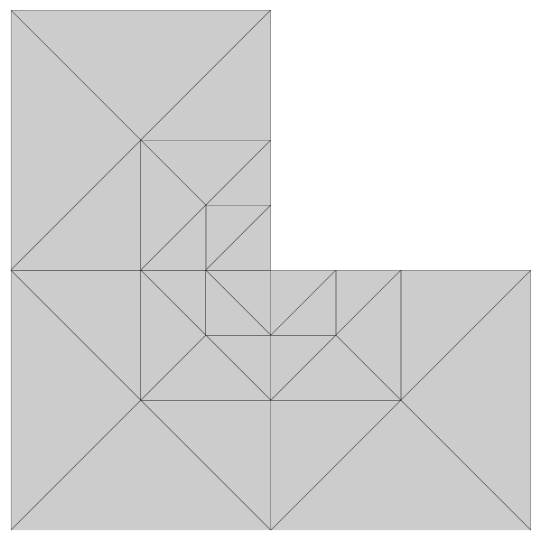
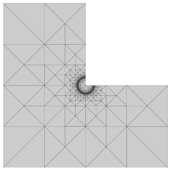
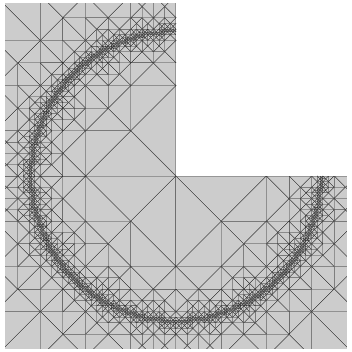
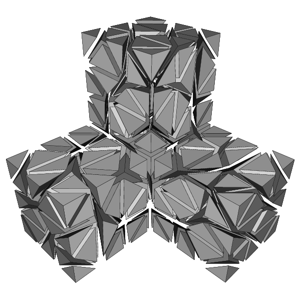
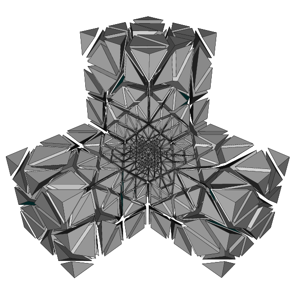
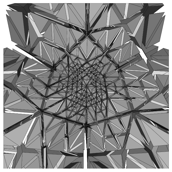
Figure 4. Examples illustrating the 2D and 3D adaptive mesh refinement algorithms in MC. The right-most figure in each row shows a close-up of the area where most of the refinement occured in each example.

MC employs the error indicators derived in Section 2.3 adaptive solution of nonlinear elliptic systems of the form (2.5)–(2.7). In particular, the indicators are used to adaptively construct Galerkin solutions satisfying (2.33), which approximate weak solutions satisfying (2.14). MC can be directed to use either the local residual indicator (2.2) together with the principle of error equi-distribution, or the duality-based weighted residual indicator (2.3), again together with equi-distribution.

Of course, we can’t perform the integrals in (2.2) or (2.3) exactly in most cases, so we employ quadrature in MC. Another option is to project the data onto the finite element spaces involved and then to perform the integrals exactly; this approach is analyzed carefully in [90]. Note that $\eta_{s}$ is computable by quadrature, since all terms appearing in the definition depend only on the (available) computed solution $u_{h}$. In particular, each of the terms

$$A^{ia}(x^{b},(u_{h})^{j},(u_{h})^{k}_{~{};c})_{;a},~{}~{}~{}A^{ia}(x^{b},(u_{h})^{j},(u_{h})^{k}_{~{};c})n_{a},$$

$$B^{i}(x^{b},(u_{h})^{j},(u_{h})^{k}_{~{};c}),~{}~{}~{}C^{i}(x^{b},(u_{h})^{j},(u_{h})^{k}_{~{};c}),$$

depend only on $u_{h}$, its first derivatives, and the normal vector $n_{q}$ (which is known from simple geometrical calculations). All of the terms but the first are already provided by the user as part of the weak form $\langle F(u),v\rangle$ required to use MC. The only problematic term is the first one; this represents the strong form of the principle part of the equation, and must be supplied by the user as a separate piece of information.

In order to understand this more completely, we will briefly describe some of the problem specification details in MC. To use MC to discretize problems of the form (2.14)–(2.15), the user is expected to provide the Dirichlet function $\bar{u}$ by providing the function $E$ in (2.7). In addition, the user provides the nonlinear weak form:

$$\langle F(u),v\rangle = \int_{{\mathcal{M}}}{\mathcal{G}}_{ij}(A^{ia}v^{j}_{~{};a}+B^{i}v^{j})~{}dx+\int_{\partial_{N}{\mathcal{M}}}{\mathcal{G}}_{ij}C^{i}v^{j}~{}ds$$ (3.2)

$$= \int_{{\mathcal{M}}}F_{0}(u)(v)~{}dx+\int_{\partial_{N}{\mathcal{M}}}F_{1}(u)(v)~{}ds,$$

by providing the integrand function $F_{t}(u)(v)$ defined as:

$$F_{t}(u)(v)~{}=~{}\left\{\begin{array}[]{ll}{\mathcal{G}}_{ij}(A^{ia}v^{j}_{~{};a}+B^{i}v^{j}),&~{}~{}\text{if}~{}t=0,\\ {\mathcal{G}}_{ij}C^{i}v^{j},&~{}~{}\text{if}~{}t=1.\\ \end{array}\right.$$ (3.3)

In order to use the inexact Newton iteration in MC to produce a Petrov-Galerkin approximation satisfying (2.33), the user must also provide a corresponding bilinear linearization form:

$$\langle DF(u)w,v\rangle=\int_{{\mathcal{M}}}DF_{0}(u)(w,v)~{}dx+\int_{\partial_{N}{\mathcal{M}}}DF_{1}(u)(w,v)~{}ds,$$ (3.4)

where the integrand function $DF_{t}(u)(w,v)$ is defined through Gateaux differentiation as described in Section 2.1. In order to use the a posteriori error estimator in MC, the user must provide an additional vector-valued function $SF_{t}(u)$, defined as:

$$SF_{t}(u)~{}=~{}\left\{\begin{array}[]{ll}B^{i}-A^{ia}_{~{}~{};a},&~{}~{}\text{if}~{}t=0,\\ C^{i}+A^{ia}n_{a},&~{}~{}\text{if}~{}t=1,\\ A^{ia}n_{a},&~{}~{}\text{if}~{}t=2.\\ \end{array}\right.$$ (3.5)

The key point that must be emphasized here is the following: since MC employs quadrature to evaluate the integrals appearing in each of (3.2), (3.4), and (2.2), the user-provided functions $F_{t}(u)(v)$, $DF_{t}(u)(w,v)$, and $SF_{t}(u)$ only need to be evaluated at a single point $x^{p}\in{\mathcal{M}}$ at a time. In other words, the user can simply evaluate the expressions in (3.3) and in (3.5) as if they were point vectors and point tensors, rather than vector and tensor fields. This is one of the most powerful features of MC, and of nonlinear finite element software in general. It implies that the user-defined functions $F_{t}(u)(v)$, $DF_{t}(u)(w,v)$, and $SF_{t}(u)$ can usually be implemented to appear in software exactly as they do on paper.

The remaining quantities appearing in the estimator (2.2), namely the normal vector $n_{q}$ and the mesh parameters $h_{s}$ and $h_{f}$, are completely geometrical and can be computed from the local simplex geometry information. The indicator is very inexpensive when compared to the typical cost of producing the discrete solution $u_{h}$ itself; the number of function evaluations and arithmetic operations (for performing quadrature) is always linear in the total number of simplices. Moreover, the indicator is completely local; it can be computed chart-wise when multiple coordinate systems are employed. These ideas are explored more fully in [53].

3.4. Solution of linear and nonlinear systems in MC

When a system of nonlinear finite element equations must be solved in MC, the global inexact-Newton Algorithm 2.2.2 is employed, where the linearization systems are solved by linear multilevel methods. When necessary, the Newton procedure in Algorithm 2.2.2 is supplemented with a user-defined normalization equation for performing an augmented system continuation algorithm. The linear systems arising as the Newton equations in each iteration of Algorithm 2.2.2 are solved using a completely algebraic multilevel algorithm. Either refinement-generated prolongation matrices $P_{k}$, or user-defined prolongation matrices $P_{k}$ in a standard YSMP-row-wise sparse matrix format, are used to define the multilevel hierarchy algebraically. In particular, once the single “fine” mesh is used to produce the discrete nonlinear problem $F(u)=0$ along with its linearization $Au=f$ for use in the Newton iteration in Algorithm 2.2.2, a $J$-level hierarchy of linear problems is produced algebraically using the following recursion:

$$A_{k+1}=P_{k}^{T}A_{k}P_{k},\ \ \ \ \ \ \ \ k=1,\ldots,J-1,\ \ \ \ \ \ \ \ A_{1}\equiv A.$$

As a result, the underlying multilevel algorithm is provably convergent in the case of self-adjoint-positive matrices [58]. Moreover, the multilevel algorithm has provably optimal $O(N)$ convergence properties under the standard assumptions for uniform refinements [94], and is nearly-optimal $O(N\log N)$ under very weak assumptions on adaptively refined problems [12, 2]. In the adaptive setting, a stabilized (approximate wavelet) hierarchical basis method is employed [2]. External software can also be used to generate the prolongation matrices, so that a number of different graph theory-based algebraic multilevel coarsening algorithms may be used to generate the subspace hierarchy.

Coupled with the superlinear convergence properties of the outer inexact Newton iteration in Algorithm 2.2.2, this leads to an overall complexity of $O(N)$ or $O(N\log N)$ for the solution of the discrete nonlinear problems in Step 1 of Algorithm 2.2.1. Combining this low-complexity solver with the judicious placement of unknowns only where needed due to the error estimation in Step 2 and the subdivision algorithm in Steps 3-6 of Algorithm 2.2.1, leads to a very effective low-complexity approximation technique for solving a general class of nonlinear elliptic systems on 2- and 3-manifolds.

3.5. Parallel computing in MC: The Parallel Partition of Unity Method (PPUM)

MC incorporates a new approach to the use of parallel computers with adaptive finite element methods, based on combining the Partition of Unity Method (PUM) of Babuška and Melenk [5] with local error estimate techniques of Xu and Zhou [97]. The algorithm, which we refer to as the Parallel Partition of Unity Method (PPUM), is described in detail in [9, 13]. The idea of the algorithm is as follows.

• (PPUM - Parallel Partition of Unity Method [9])

  1. Discretize and solve the problem using a global coarse mesh.

  2. Compute a posteriori error estimates using the coarse solution, and decompose the mesh to achieve equal error using weighted spectral or inertial bisection.

  3. Give the entire mesh to a collection of processors, where each processor will perform a completely independent solve-estimate-refine loop (Step 2 through Step 6 in Algorithm 2.2.1), restricting local refinement to only an assigned portion of the domain. The portion of the domain assigned to each processor coincides with one of the domains produced by spectral bisection with some overlap (produced by conformity algorithms, or by explicitly enforcing substantial overlap). When a processor has reached an error tolerance locally, computation stops on that processor.

  4. Combine the independently produced solutions using a partition of unity subordinate to the overlapping subdomains.

While the algorithm above seems to ignore the global coupling of the elliptic problem, some recent theoretical results [97] support this as provably good, and even optimal in some cases. The principle idea underlying the results in [97] is that while elliptic problems are globally coupled, this global coupling is essentially a “low-frequency” coupling, and can be handled on the initial mesh which is much coarser than that required for approximation accuracy considerations. This idea has been exploited, for example, in [95, 96], and is in fact why the construction of a coarse problem in overlapping domain decomposition methods is the key to obtaining convergence rates which are independent of the number of subdomains (c.f. [94]). A more complete description can be found in [9], along with examples using MC and the 2D adaptive finite element package PLTMG [10]. An analysis of the global $L^{2}$- and $H^{1}$-error in solutions produced by the algorithm appears in the next section. An example showing the types of local refinements that occur within each subdomain is depicted in Figure 5.

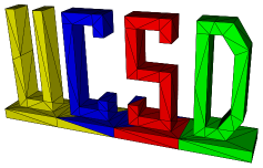
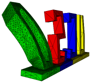
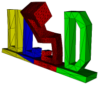
Figure 5. An example showing the types of local refinements that are created by PPUM.

3.6. Global $L^{2}$- and $H^{1}$-error estimates for PPUM

In order to analyze the error behavior in PPUM, we first review the partition of unity method (PUM) of Babuška and Melenk [5]. Let $\Omega\subset{\mathbb{R}}^{d}$ be an open set and let $\{\Omega_{i}\}$ be an open cover of $\Omega$ with a bounded local overlap property: For all $x\in\Omega$, there exists a constant $M$ such that

$$\sup_{i}\{~{}i~{}|~{}x\in\Omega_{i}~{}\}\leq M.$$ (3.6)

A Lipschitz partition of unity $\{\phi_{i}\}$ subordinate to the cover $\{\Omega_{i}\}$ satisfies the following five conditions:

$$\sum_{i}\phi_{i}(x) \equiv 1,~{}~{}~{}\forall x\in\Omega,$$ (3.7)

$$\phi_{i} \in C^{k}(\Omega)~{}~{}~{}\forall i,~{}~{}~{}(k\geq 0),$$ (3.8)

$$\sup\phi_{i} \subset \overline{\Omega}_{i},~{}~{}~{}\forall i,$$ (3.9)

$$\|\phi_{i}\|_{L^{\infty}(\Omega)} \leq C_{\infty},~{}~{}~{}\forall i,$$ (3.10)

$$\|\nabla\phi_{i}\|_{L^{\infty}(\Omega)} \leq \frac{C_{G}}{\text{diam}(\Omega_{i})},~{}~{}~{}\forall i.$$ (3.11)

The partition of unity method (PUM) builds an approximation $u_{ap}=\sum_{i}\phi_{i}v_{i}$ where the $v_{i}$ are taken from the local approximation spaces:

$$V_{i}\subset C^{k}(\Omega\cap\Omega_{i})\subset H^{1}(\Omega\cap\Omega_{i}),~{}~{}~{}\forall i,~{}~{}~{}(k\geq 0).$$ (3.12)

The following simple lemma makes possible several useful results.

Lemma 3.1.

Let $w,w_{i}\in H^{1}(\Omega)$ with $\text{supp}~{}w_{i}\subseteq\overline{\Omega\cap\Omega_{i}}$. Then

$$\sum_{i}\|w\|_{H^{k}(\Omega_{i})}^{2} \leq M\|w\|_{H^{k}(\Omega)}^{2},~{}~{}~{}~{}k=0,1$$

$$\|\sum_{i}w_{i}\|_{H^{k}(\Omega)}^{2} \leq M\sum_{i}\|w_{i}\|_{H^{k}(\Omega\cap\Omega_{i})}^{2},~{}~{}~{}~{}k=0,1$$

Proof.

The proof follows from (3.6) and (3.7)–(3.11); see [5].∎∎

The basic approximation properties of PUM are as follows.

Theorem 3.2 (Babuška and Melenk [5]).

If the local spaces $V_{i}$ have the following approximation properties:

$$\|u-v_{i}\|_{L^{2}(\Omega\cap\Omega_{i})} \leq \epsilon_{0}(i),~{}~{}~{}\forall i,$$

$$\|\nabla(u-v_{i})\|_{L^{2}(\Omega\cap\Omega_{i})} \leq \epsilon_{1}(i),~{}~{}~{}\forall i,$$

then the following a priori global error estimates hold:

$$\|u-u_{ap}\|_{L^{2}(\Omega)} \leq \sqrt{M}C_{\infty}\left(\sum_{i}\epsilon_{0}^{2}(i)\right)^{1/2},$$

$$\|\nabla(u-u_{ap})\|_{L^{2}(\Omega)} \leq \sqrt{2M}\left(\sum_{i}\left(\frac{C_{G}}{\text{diam}(\Omega_{i})}\right)^{2}\epsilon_{1}^{2}(i)+C_{\infty}^{2}\epsilon_{0}^{2}(i)\right)^{1/2}.$$

Proof.

This follows from Lemma 3.1 by taking $u-u_{ap}=\sum_{i}\phi_{i}(u-v_{i})$ and $w_{i}=\phi_{i}(u-v_{i})$.∎∎

We now give a global $H^{1}$-error estimate of the PPUM adaptive algorithm proposed in [9]. We can view PPUM as building a PUM approximation $u_{pp}=\sum_{i}\phi_{i}v_{i}$ where the $v_{i}$ are taken from the local spaces:

$$V_{i}={\mathcal{X}}_{i}V_{i}^{g}\subset C^{k}(\Omega\cap\Omega_{i})\subset H^{1}(\Omega\cap\Omega_{i}),~{}~{}~{}\forall i,~{}~{}~{}(k\geq 0),$$ (3.13)

where ${\mathcal{X}}_{i}$ is the characteristic function for $\Omega_{i}$, and where

$$V_{i}^{g}\subset C^{k}(\Omega)\subset H^{1}(\Omega),~{}~{}~{}\forall i,~{}~{}~{}(k\geq 0).$$ (3.14)

In PPUM, the global spaces $V_{i}^{g}$ in (3.13)–(3.14) are built from locally enriching an initial coarse global space $V_{0}$ by locally adapting the finite element mesh on which $V_{0}$ is built. (This is in contrast to classical overlapping schwarz domain decomposition methods where local spaces are often built through enrichment of $V_{0}$ by locally adapting the mesh on which $V_{0}$ is built, and then removing the portions of the mesh exterior to the adapted region.) The PUM space $V$ is then

$$V = \left\{~{}v~{}|~{}v=\sum_{i}\phi_{i}v_{i},~{}~{}~{}v_{i}\in V_{i}~{}\right\}$$

$$= \left\{~{}v~{}|~{}v=\sum_{i}\phi_{i}{\mathcal{X}}_{i}v_{i}^{g}=\sum_{i}\phi_{i}v_{i}^{g},~{}~{}~{}v_{i}^{g}\in V_{i}^{g}~{}\right\}\subset H^{1}(\Omega).$$

Consider now the following linear elliptic problem in the plane:

$$\begin{array}[]{rcl}-\nabla\cdot(a\nabla u)&=&f~{}\text{in}~{}\Omega,\\ u&=&0~{}\text{on}~{}\partial\Omega,\end{array}$$ (3.15)

where $a_{ij}\in W^{1,\infty}(\Omega)$, $f\in L^{2}(\Omega)$, $a_{ij}\xi_{i}\xi_{j}\geq a_{0}>0$, $\forall\xi_{i}\neq 0$, where $\Omega\subset{\mathbb{R}}^{2}$ is a convex polygon. (The results below also hold more generally for classes of two- and three-dimensional nonlinear problems.) A weak formulation is:

$$\text{Find}~{}u\in H^{1}_{0}(\Omega)~{}\text{such~{}that}~{}\langle F(u),v\rangle=0,~{}~{}~{}\forall v\in H^{1}_{0}(\Omega),$$

where

$$\langle F(u),v\rangle=\int_{\Omega}a\nabla u\cdot\nabla v~{}dx-\int_{\Omega}fv~{}dx.$$

The PUM is usually used to solve a PDE as a Galerkin method in the globally coupled PUM space (cf. [46]):

$$\text{Find}~{}u_{ap}\in V\subset H^{1}_{0}(\Omega)~{}\text{s.t.}~{}\langle F(u_{ap}),v\rangle=0,~{}\forall v\in V\subset H^{1}_{0}(\Omega).$$

In contrast, PPUM proposed in [9] builds an approximation $u_{pp}$ from decoupled local Galerkin solutions:

$$u_{pp}=\sum_{i}\phi_{i}u_{i}=\sum_{i}\phi_{i}u_{i}^{g},$$ (3.16)

where each $u_{i}^{g}$ satisfies:

$$\text{Find}~{}u_{i}^{g}\in V_{i}^{g}~{}\text{such~{}that}~{}\langle F(u_{i}^{g}),v_{i}^{g}\rangle=0,~{}~{}~{}\forall v_{i}^{g}\in V_{i}^{g}.$$ (3.17)

We have the following global error estimate for the approximation $u_{pp}$ in (3.16) built from (3.17) using the local PPUM parallel algorithm.

Theorem 3.3.

Assume the solution to (3.15) satisfies $u\in H^{1+\alpha}(\Omega)$, $\alpha>0$, and assume that quasi-uniform meshes of sizes $h$ and $H>h$ are used for $\Omega_{i}^{0}$ and $\Omega\backslash\Omega_{i}^{0}$ respectively. If $\text{diam}(\Omega_{i})\geq 1/Q>0~{}~{}\forall i$, then the global solution $u_{pp}$ in (3.16) produced by the PPUM Algorithm 3.5 satisfies the following global error bounds:

$$\|u-u_{pp}\|_{L^{2}(\Omega)} \leq \sqrt{PM}C_{\infty}\left(C_{1}h^{\alpha}+C_{2}H^{1+\alpha}\right),$$

$$\|\nabla(u-u_{pp})\|_{L^{2}(\Omega)} \leq \sqrt{2PM(Q^{2}C_{G}^{2}+C_{\infty}^{2})}\left(C_{1}h^{\alpha}+C_{2}H^{1+\alpha}\right),$$

where $P=$ number of local spaces $V_{i}$. Further, if $H\leq h^{\alpha/(1+\alpha)}$ then:

$$\|u-u_{pp}\|_{L^{2}(\Omega)} \leq \sqrt{PM}C_{\infty}\max\{C_{1},C_{2}\}h^{\alpha},$$

$$\|\nabla(u-u_{pp})\|_{L^{2}(\Omega)} \leq \sqrt{2PM(Q^{2}C_{G}^{2}+C_{\infty}^{2})}\max\{C_{1},C_{2}\}h^{\alpha},$$

so that the solution produced by Algorithm 3.5 is of optimal order in the $H^{1}$-norm.

Proof.

Viewing PPUM as a PUM gives access to the PUM a priori estimates in Theorem 3.2; these require local estimates of the form:

$$\|u-u_{i}\|_{L^{2}(\Omega\cap\Omega_{i})}=\|u-u_{i}^{g}\|_{L^{2}(\Omega\cap\Omega_{i})} \leq \epsilon_{0}(i),$$

$$\|\nabla(u-u_{i})\|_{L^{2}(\Omega\cap\Omega_{i})}=\|\nabla(u-u_{i}^{g})\|_{L^{2}(\Omega\cap\Omega_{i})} \leq \epsilon_{1}(i).$$

Such local a priori estimates are available for problems of the form (3.15) [74, 97]. They can be shown to take the following form:

$$\|u-u_{i}^{g}\|_{H^{1}(\Omega_{i}\cap\Omega)}\leq C\left(\inf_{v_{i}^{0}\in V_{i}^{0}}\|u-v_{i}^{0}\|_{H^{1}(\Omega_{i}^{0}\cap\Omega)}+\|u-u_{i}^{g}\|_{L^{2}(\Omega)}\right)$$

where

$$V_{i}^{0}\subset C^{k}(\Omega_{i}^{0}\cap\Omega)\subset H^{1}(\Omega_{i}\cap\Omega),$$

and where

$$\Omega_{i}\subset\subset\Omega_{i}^{0},\ \ \ \ \ \Omega_{ij}=\Omega_{i}^{0}\bigcap\Omega_{i}^{0},\ \ \ \ \ |\Omega_{ij}|\approx|\Omega_{i}|\approx|\Omega_{j}|.$$

Since we assume $u\in H^{1+\alpha}(\Omega)$, $\alpha>0$, and since quasi-uniform meshes of sizes $h$ and $H>h$ are used for $\Omega_{i}^{0}$ and $\Omega\backslash\Omega_{i}^{0}$ respectively, we have:

$$\|u-u_{i}^{g}\|_{H^{1}(\Omega_{i}\cap\Omega)} = \left(\|u-u_{i}^{g}\|_{L^{2}(\Omega_{i}\cap\Omega)}^{2}+\|\nabla(u-u_{i}^{g})\|_{L^{2}(\Omega_{i}\cap\Omega)}^{2}\right)^{1/2}$$

$$\leq C_{1}h^{\alpha}+C_{2}H^{1+\alpha}.$$

I.e., in this setting we can use $\epsilon_{0}(i)=\epsilon_{1}(i)=C_{1}h^{\alpha}+C_{2}H^{1+\alpha}$. The a priori PUM estimates in Theorem 3.2 then become:

$$\|u-u_{pp}\|_{L^{2}(\Omega)} \leq \sqrt{M}C_{\infty}\left(\sum_{i}(C_{1}h^{\alpha}+C_{2}H^{1+\alpha})^{2}\right)^{1/2},$$

$$\|\nabla(u-u_{pp})\|_{L^{2}(\Omega)} \leq \sqrt{2M}$$

$$\cdot\left(\left[\sum_{i}\left(\frac{C_{G}}{\text{diam}(\Omega_{i})}\right)^{2}+C_{\infty}^{2}\right](C_{1}h^{\alpha}+C_{2}H^{1+\alpha})^{2}\right)^{1/2}.$$

If $P=$ number of local spaces $V_{i}$, and if $\text{diam}(\Omega_{i})\geq 1/Q>0~{}~{}\forall i$, this is simply:

$$\|u-u_{pp}\|_{L^{2}(\Omega)} \leq \sqrt{PM}C_{\infty}\left(C_{1}h^{\alpha}+C_{2}H^{1+\alpha}\right),$$

$$\|\nabla(u-u_{pp})\|_{L^{2}(\Omega)} \leq \sqrt{2PM(Q^{2}C_{G}^{2}+C_{\infty}^{2})}\left(C_{1}h^{\alpha}+C_{2}H^{1+\alpha}\right).$$

If $H\leq h^{\alpha/(1+\alpha)}$ then $u_{pp}$ from PPUM is asymptotically as good as a global Galerkin solution when the error is measured in the $H^{1}$-norm.∎∎

Estimates similar to Theorem 3.3 appear in [97] for a variety of related parallel algorithms. Note that improving the estimates in the $L^{2}$-norm is not possible; the required local estimates simply do not hold. Improving the solution quality in the $L^{2}$-norm would require more global information.

3.7. Availability of MC and the supporting tools MALOC and SG

MC is built on top of a low-level portability library called MALOC (Minimal Abstraction Layer for Object-oriented C). Most of the images appearing in this paper were produced using a software tool called SG (Socket Graphics), which is also built on top of MALOC. MALOC, MC, and SG were developed by the author over several years, with generous contributions from a number of colleagues. MALOC, MC, and SG are freely redistributable under the GNU General Public License (GPL), and the source code for all three packages is freely available at the following website:

http://www.scicomp.ucsd.edu/~mholst/

MALOC, MC, and SG, as well as a fully functional MATLAB version of MC called MCLab, are part of a larger project called FETK (The Finite Element Toolkit). Information about FETK can be found at:

http://www.fetk.org

4. Example: The Hamiltonian and momentum constraints in the Einstein equations

The evolution of the gravitational field was conjectured by Einstein to be governed by twelve coupled first-order hyperbolic equations for the metric of space-time and its time derivative, where the evolution is constrained for all time by a coupled four-component elliptic system. This four-component elliptic system consists of a nonlinear scalar Hamiltonian constraint, and a linear 3-vector momentum constraint. The evolution and constraint equations, similar in some respects to Maxwell’s equations, are collectively referred to as the Einstein equations. Solving the constraint equations numerically, separately or together with the evolution equations, is currently of great interest to the physics community (cf. [56, 55, 26] for more detailed discussions of this application).

The Hamiltonian and momentum constraints in the Einstein equations, taken separately or together as a coupled system, have the form (2.5)–(2.7). Allowing for both Dirichlet and Robin boundary conditions as are typically used in black hole and neutron star models (cf. [56, 55, 26]), the strong form can be written as:

$$\hat{\Delta}\phi = \frac{1}{8}\hat{R}\phi+\frac{1}{12}({\rm tr}K)^{2}\phi^{5}$$

$$-\frac{1}{8}({}^{*}\!\!\hat{A}_{ab}+(\hat{L}W)_{ab})^{2}\phi^{-7}-2\pi\hat{\rho}\phi^{-3}~{}~{}\text{in}~{}{\mathcal{M}},$$

$$\hat{n}_{a}\hat{D}^{a}\phi+c\phi = z~{}\text{on}~{}\partial_{1}{\mathcal{M}},$$ (4.2)

$$\phi = f~{}\text{on}~{}\partial_{0}{\mathcal{M}},$$ (4.3)

$$\hat{D}_{b}(\hat{L}W)^{ab} = \frac{2}{3}\phi^{6}\hat{D}^{a}{\rm tr}K+8\pi\hat{j}^{a}~{}~{}\text{in}~{}{\mathcal{M}},$$ (4.4)

$$(\hat{L}W)^{ab}\hat{n}_{b}+C^{a}_{~{}b}W^{b} = Z^{a}~{}\text{on}~{}\partial_{1}{\mathcal{M}},$$ (4.5)

$$W^{a} = F^{a}~{}~{}\text{on}~{}\partial_{0}{\mathcal{M}},$$ (4.6)

where the following standard notation has been employed:

$$\hat{\Delta}\phi = \hat{D}_{a}\hat{D}^{a}\phi,$$

$$(\hat{L}W)^{ab} = \hat{D}^{a}W^{b}+\hat{D}^{b}W^{a}-\frac{2}{3}\hat{\gamma}^{ab}\hat{D}_{c}W^{c},$$

$${\rm tr}K = \gamma^{ab}K_{ab},$$

$$(C_{ab})^{2} = C^{ab}C_{ab}.$$

The symbols in the equations ($\hat{R}$, $K$, ${}^{*}\!\!\hat{A}_{ab}$, $\hat{\rho}$, $\hat{j}^{a}$, $z$, $Z^{a}$, $f$, $F^{a}$, $c$, and $C^{a}_{b}$) represent various physical parameters, and are described in detail in [56, 55, 26] and the referenences therein.

Equations (4)–(4.6) are known to be well-posed only for restricted problem data and manifold topologies [77, 75, 76]. Below we will present two well-posedness results from [56] which hold under certain assumptions. Note that if multiple solutions in the form of folds or bifurcations are present in solutions of (4)–(4.6) then path-following numerical methods will be required for numerical solution [62, 63].

4.1. Weak formulation, linearization, and well-posedness

Both the Hamiltonian constraint (4) and the momentum constraint (4.4), taken separately or as a system, fall into the class of second-order divergence-form elliptic systems of tensor equations in (2.5)–(2.7). Derivation of the weak formulation produces a weak system of the form (2.14)–(2.15), with some interesting twists along the way described in [56]. Following the notation in [56], we employ a background (or conformal) metric $\hat{\gamma}_{ab}$ to define the volume element $dx=\sqrt{\text{det}~{}\hat{\gamma}_{ab}}~{}dx^{1}dx^{2}dx^{3}$ and the corresponding boundary volume element $ds$, and for use as the manifold connection for covariant differentiation. The notation for covariant differentiation using the conformal connection will be denoted $\hat{D}_{a}$ to be consistent with the relativity literature, and the various quantities from Section 2.1 will now be hatted to denote use of this conformal metric. For example, the unit normal to $\partial{\mathcal{M}}$ will now be denoted $\hat{n}^{a}$.

Ordering the Hamiltonian constraint first in the system (2.5), and defining the product metric ${\mathcal{G}}_{ij}$ and the vectors $u^{i}$ and $v^{j}$ appearing in (2.11) and (2.15) as:

$${\mathcal{G}}_{ij}=\left[\begin{array}[]{ccc}1&0\\ 0&g_{ab}\\ \end{array}\right],~{}~{}~{}~{}~{}u^{i}=\left[\begin{array}[]{c}\phi\\ W^{a}\\ \end{array}\right],~{}~{}~{}~{}~{}v^{j}=\left[\begin{array}[]{c}\psi\\ V^{b}\\ \end{array}\right],$$

it is shown in [56] that the coupled Hamiltonian and momentum constraints have a coupled weak formulation in the form of (2.14), where the form definition is as follows:

$$\langle F(u),v\rangle=\langle F([\phi,W^{a}]),[\psi,V^{a}]\rangle=\langle F_{\text{H}}(\phi),\psi\rangle+\langle F_{\text{M}}(W^{a}),V^{a}\rangle.$$ (4.7)

The individual Hamiltonian form is shown in [56] to be:

$$\langle F_{\text{H}}(\phi),\psi\rangle=\int_{{\mathcal{M}}}\hat{D}_{a}\phi\hat{D}^{a}\psi~{}dx+\int_{{\mathcal{M}}}P^{\prime}(\phi)\psi~{}dx$$ (4.8)

$$+\int_{\partial_{1}{\mathcal{M}}}(c\phi-z)\psi~{}ds,$$

where

$$P^{\prime}(\phi)=\frac{1}{8}\hat{R}\phi+\frac{1}{12}({\rm tr}K)^{2}\phi^{5}-\frac{1}{8}({}^{*}\!\!\hat{A}_{ab}+(\hat{L}W)_{ab})^{2}\phi^{-7}-2\pi\hat{\rho}\phi^{-3},$$ (4.9)

and the momentum form is shown in [56] to be:

$$\langle F_{\text{M}}(W^{a}),V^{a}\rangle=\int_{{\mathcal{M}}}\left(2\mu(\hat{E}W)^{ab}(\hat{E}V)_{ab}+\lambda\hat{D}_{a}W^{a}\hat{D}_{b}V^{b}\right)~{}dx$$ (4.10)

$$+\int_{{\mathcal{M}}}\left(\frac{2}{3}\phi^{6}\hat{D}^{a}{\rm tr}K+8\pi\hat{j}^{a}\right)V_{a}~{}dx\int_{\partial_{1}{\mathcal{M}}}(C^{a}_{~{}b}W^{b}-Z^{a})V_{a}~{}ds,$$

where $\mu=1$, $\lambda=-2/3$, and where the deformation tensor $(\hat{E}V)^{ab}$ is the symmetrized gradient:

$$(\hat{E}V)^{ab}=\frac{1}{2}\left(\hat{D}^{b}V^{a}+\hat{D}^{a}V^{b}\right).$$ (4.11)

The Gateaux-derivative of the nonlinear weak form $\langle F(\cdot),\cdot\rangle$ in equation (4.7) above is needed for use in Newton-like iterative solution methods such as Algorithm 2.2.2. Defining an arbitrary variation direction $w=[\xi,X^{a}]$, it is shown in [56] that the Gateaux-derivative takes the following form (for fixed $[\phi,W^{a}]$), linear separately in each of the variables $[\xi,X^{a}]$ and $[\psi,V^{a}]$:

$$\langle DF([\phi,W^{a}])[\xi,X^{a}],[\psi,V^{a}]\rangle=$$ (4.12)

$$\int_{\partial_{1}{\mathcal{M}}}\left(c\xi\psi+C^{a}_{~{}b}X^{b}V_{a}\right)~{}ds$$

$$+\int_{{\mathcal{M}}}\left(\hat{D}_{a}\xi\hat{D}^{a}\psi+2\mu(\hat{E}X)^{ab}(\hat{E}V)_{ab}+\lambda\hat{D}_{a}X^{a}\hat{D}_{b}V^{b}\right)~{}dx$$

$$+\int_{{\mathcal{M}}}\left(\frac{1}{8}\hat{R}+\frac{5}{12}({\rm tr}K)^{2}\phi^{4}+\frac{7}{8}({}^{*}\!\!\hat{A}_{ab}+(\hat{L}W)_{ab})^{2}\phi^{-8}+6\pi\hat{\rho}\phi^{-4}\right)\xi\psi~{}dx$$

$$-\int_{{\mathcal{M}}}\left(\frac{1}{4}({}^{*}\!\!\hat{A}_{ab}+(\hat{L}W)_{ab})\phi^{-7}\right)(\hat{L}X)^{ab}\psi~{}dx+\int_{{\mathcal{M}}}\left(4\phi^{5}\hat{D}^{a}{\rm tr}K\right)V_{a}\xi~{}dx.$$

Now that the nonlinear weak form $\langle F(\cdot),\cdot\rangle$ and the associated bilinear linearization form $\langle DF(\cdot)\cdot,\cdot\rangle$ are defined and can be evaluated using numerical quadrature, the assembly of the nonlinear residual as well as linearizations about any point can be performed precisely as outlined above for a generic nonlinear finite element method. Again, once we have the weak formulation and a linearization, the discretization in MC is automatic and generic. Although the forms $\langle F(\cdot),\cdot\rangle$ and $\langle DF(\cdot)\cdot,\cdot\rangle$ above appear somewhat complicated in the case of the constraint equations, the discretization in MC involves simply evaluating the integrands for use in quadrature formulae.

We now state two new existence and uniqueness results for the Hamiltonian and momentum constraints which were established recently in [56]. A number of assumptions on the problem data are required.

Assumption 4.1.

We assume that ${\mathcal{M}}$ is a connected compact Riemannian $3$-manifold with Lipschitz-continuous boundary $\partial{\mathcal{M}}$. We also assume that the data has the following properties:

$$\hat{\gamma}_{ab}\in W^{1,\infty}({\mathcal{M}}),~{}~{}K^{ab}\in W^{1,6/5}({\mathcal{M}}),~{}~{}\phi\in L^{\infty}({\mathcal{M}}),~{}~{}\overline{W}^{a}\in H^{1}({\mathcal{M}}),$$

$$\hat{j}^{a}\in H^{-1}({\mathcal{M}}),~{}~{}C^{a}_{~{}b}\in L^{2}(\partial_{1}{\mathcal{M}}),~{}~{}Z^{a}\in L^{4/3}(\partial_{1}{\mathcal{M}}),~{}~{}F^{a}\in H^{1/2}(\partial_{0}{\mathcal{M}}),$$

where $\overline{W}^{a}|_{\partial_{0}{\mathcal{M}}}=F^{a}$ in the trace sense, and where for some constant $\sigma>0$,

$$\int_{\partial_{1}{\mathcal{M}}}C^{a}_{~{}b}V^{b}V_{a}~{}dx\geq\sigma\|V^{a}\|_{L^{2}(\partial_{1}{\mathcal{M}})}^{2},~{}~{}\forall~{}V^{a}\in L^{4}(\partial_{1}{\mathcal{M}}).$$

Assumption 4.2.

We assume that ${\mathcal{M}}$ is a connected compact Riemannian $3$-manifold with Lipschitz-continuous boundary $\partial{\mathcal{M}}$, where $\text{meas}(\partial_{0}{\mathcal{M}})>0$. We also assume that the data has the following properties:

$$\hat{\gamma}_{ab}\in W^{1,\infty}({\mathcal{M}}),~{}~{}K^{ab}\in L^{\infty}({\mathcal{M}}),~{}~{}W^{a}\in W^{1,\infty}({\mathcal{M}}),~{}~{}\overline{\phi}\in H^{1}({\mathcal{M}})\cap L^{\infty}({\mathcal{M}}),$$

$$\hat{R},{}^{*}\!\!\hat{A}_{ab},\rho\in L^{\infty}({\mathcal{M}}),~{}~{}c,z\in L^{\infty}(\partial_{1}{\mathcal{M}}),~{}~{}f\in H^{1/2}(\partial_{0}{\mathcal{M}})\cap L^{\infty}(\partial_{0}{\mathcal{M}}),$$

where $\bar{\phi}|_{\partial_{0}{\mathcal{M}}}=f$ in the trace sense, and

$$0<\inf_{\partial_{0}{\mathcal{M}}}f\leq f\leq\sup_{\partial_{0}{\mathcal{M}}}f<\infty,~{}~{}~{}~{}a.e.~{}\text{in}~{}\partial_{0}{\mathcal{M}},$$

$$\rho\geq 0,~{}~{}a.e.~{}\text{in}~{}{\mathcal{M}},~{}~{}c\geq 0,~{}~{}z=0,~{}~{}a.e.~{}\text{on}~{}\partial_{1}{\mathcal{M}}.$$

Theorem 4.3.

Let Assumption 4.1 hold. Then there exists a unique solution $W^{a}\in\overline{W}^{a}+H^{1}_{0,D}({\mathcal{M}})$ to the momentum constraint equation (4.4)–(4.6) which depends continuously on the problem data. Moreover, $U^{a}=W^{a}-\overline{W}^{a}\in H^{1}_{0,D}({\mathcal{M}})$ satisfies the following a priori bound:

$$\|U^{a}\|_{H^{1}({\mathcal{M}})}\leq\|U^{a}\|_{L^{2}({\mathcal{M}})}+\frac{L}{\alpha},$$ (4.13)

where $\alpha$ is the strong ellipticity constant and $L$ is a bound on the linear functional arising in the weak form. If $\text{meas}(\partial_{0}{\mathcal{M}})>0$, then the following bound also holds:

$$\|U^{a}\|_{H^{1}({\mathcal{M}})}\leq\frac{L}{m},$$ (4.14)

where $m$ is the coercivity constant.

Proof.

The proof given in [56] is based on the use of a Riesz-Schauder alternative argument (uniqueness implies existence), which is accessible after establishing that the momentum weak form operator has a number of properties, including strong ellipticity and satisfaction of a Gårding inequality.∎∎

Theorem 4.4.

Let Assumption 4.2 hold. Then there exists a unique solution $\phi\in\bar{\phi}+H^{1}_{0,D}({\mathcal{M}})$ to the Hamiltonian constraint equation (4)–(4.3). The solution $\phi$ satisfies a priori $L^{\infty}$-bounds and is strictly positive a.e. in ${\mathcal{M}}$.

Proof.

The proof given in [56] is based on variational analysis and fixed-point arguments, after using a weak maximum principle to remove the poles at the origin in the nonlinearity. ∎∎

The two results above indicate that the momentum and Hamiltonian constraints on connected compact Riemannian manifolds with Lipschitz boundaries have well-posed weak formulations in the unweighted Sobolev spaces $H^{1}_{0,D}({\mathcal{M}})$. A small amount of additional regularity, namely the intersection of Assumptions 4.1 and 4.2, is required to give simultaneously well-posed weak formulations. Under smoothness assumptions on the boundary and coefficients, this minimal additional regularity can be shown for both $\phi$ and $W^{a}$ using elliptic regularity arguments (cf. [70] for a discussion of the linear elasticity case which can be adapted here for the momentum constraint). Unfortunately, elliptic systems such as the momentum constraint do not satisfy maximum principles analogous to the weak maximum principle derived for the (scalar) Hamiltonian constraint in [56], and as a result it is more difficult to establish $L^{\infty}$-bounds on $W^{a}$. Note that simultaneous well-posedness of the Hamiltonian and momentum constraints individually does not imply well-posedness of the coupled system. Limited results for the coupled system exist for some simplified situations; cf. [60, 59, 34, 33, 77]. Some new results for the coupled system, based on Theorems 4.3 and 4.4, appear in [56].

4.2. Quasi-optimal a priori error estimates for Galerkin approximations

In this section we consider the theory for Galerkin approximations of the Hamiltonian and momentum constraints. Following the approaches in [29, 84, 61] for related problems, we establish two abstract results, the first of which applies to linear variational problems satisfying a Gårding inequality, whereas the second result applies to monotonically nonlinear variational problems. When applied to the Hamiltonian and momentum constraints, each result will take the form:

$$\|u-u_{h}\|_{H^{1}({\mathcal{M}})}\leq C\inf_{v\in V_{h}}\|u-v\|_{H^{1}({\mathcal{M}})},$$ (4.15)

where $u_{h}$ is a Galerkin approximation such as provided by a finite element discretization, and where $V_{h}\subset H^{1}_{0,D}({\mathcal{M}})$ is the subspace of continuous piecewise polynomials defined over simplices. These results are quasi-optimal in the sense that they imply that a Galerkin solution of either the Hamiltonian or momentum constraint is within a constant of being the best approximation in the particular subspace in which the Galerkin solution lives. After giving the two abstract results along with their simple short proofs, we indicate how they can be applied to the momentum and Hamiltonian constraints in the context of Galerkin finite element methods.

While the term on the left in (4.15) is in general difficult to analyze, the term on the right represents the fundamental question addressed by classical approximation theory in normed spaces, of which much is known. To bound the term on the right from above, one picks a function in $V_{h}$ which is particularly easy to work with, namely a nodal or generalized interpolant of $u$, and then one employs standard techniques in interpolation theory. Therefore, it is clear that the importance of approximation results such as (4.15) are that they completely separate the details of the momentum and Hamiltonian constraints from the approximation theory, making available all known results on finite element interpolation of functions in Sobolev spaces (cf. [35]). There are some additional difficulties in using the standard finite element interpolation theory associated with the fact that we are working with a domain with the structure of a Riemannian 3-manifold rather than an open set in ${\mathbb{R}}^{d}$; these are being addressed in work in progress [53], and will not be discussed in detail here.

4.2.1. Approximation theory for the momentum constraint

We now give a quasi-optimal a priori error estimate which characterizes the quality of a Galerkin approximation to the solution of the momentum constraint. Quasi-optimal estimates are quite standard in the finite element approximation theory literature for V-elliptic bilinear forms, but unfortunately it is shown in [56] that the momentum constraint weak form is only V-coercive (satisfying a Gårding inequality). However, following Schatz [84] we show this is sufficient to establish similar quasi-optimal results for the momentum constraint (cf. [85, 97] for related results).

In order to derive such a result following the approach in [84], we begin with a Gelfand triple of Hilbert spaces $V\subset H\equiv H^{*}\subset V^{*}$ with continuous embedding, meaning that the pivot space $H$ and its dual space $H^{*}$ are identified through the Riesz representation theorem, and that the embedding $V\subset H$ is continuous. A consequence of this is:

$$\|u\|_{H}\leq C\|u\|_{V},~{}~{}\forall u\in V,$$ (4.16)

where we will assume that the embedding constant $C=1$ (the norm $\|\cdot\|_{V}$ can be redefined as necessary). In our setting of the momentum constraint, we have $H=L^{2}({\mathcal{M}})$ and $V=H^{1}_{0,D}({\mathcal{M}})$ generating the triple; we will stay with the abstract notation involving $H$ and $V$ for clarity. We are given the following variational problem:

$$\text{Find}~{}u\in V~{}\text{s.t.}~{}A(u,v)=F(v),~{}~{}\forall v\in V,$$ (4.17)

where the bilinear form $A(u,v):V\times V\mapsto{\mathbb{R}}$ is bounded

$$A(u,v)\leq M\|u\|_{V}\|v\|_{V},~{}~{}\forall u,v\in V,$$ (4.18)

and V-coercive (satisfying a Gårding inequality):

$$m\|u\|_{V}^{2}\leq K\|u\|_{H}^{2}+A(u,u),~{}~{}\forall u\in V,~{}~{}~{}\text{where}~{}~{}m>0,$$ (4.19)

and where the linear functional $F(v):V\mapsto{\mathbb{R}}$ is bounded and thus lies in the dual space $V^{*}$:

$$F(v)\leq L\|v\|_{V},~{}~{}\forall v\in V.$$

It is shown in [56] that the weak formulation of the momentum constraint (4.10) fits into this framework; to simplify the discussion, we have assumed that any Dirichlet function $\bar{u}$ has been absorbed into the linear functional $F(v)$ in the obvious way. Our discussion can be easily modified to include approximation of $\bar{u}$ by $\bar{u}_{h}$.

Now, we are interested in the quality of a Galerkin approximation:

$$\text{Find}~{}u_{h}\in V_{h}\subset V~{}\text{s.t.}~{}A(u_{h},v)=A(u,v)=F(v),~{}~{}\forall v\in V_{h}\subset V.$$ (4.20)

We will assume that there exists a sequence of approximation subspaces $V_{h}\subset V$ parameterized by $h$, with $V_{h_{1}}\subset V_{h_{2}}$ when $h_{2}<h_{1}$, and that there exists a sequence $\{a_{h}\}$, with $\lim_{h\rightarrow 0}a_{h}=0$, such that

$$\|u-u_{h}\|_{H}\leq a_{h}\|u-u_{h}\|_{V},~{}\text{when}~{}A(u-u_{h},v)=0,~{}\forall v\in V_{h}\subset V.$$ (4.21)

The assumption (4.21) is very natural; in our setting, it is the assumption that the error in the approximation converges to zero more quickly in the $L^{2}$-norm than in the $H^{1}$-norm. This is easily verified in the setting of piecewise polynomial approximation spaces, under very mild smoothness requirements on the solution $u$; cf. Lemmas 2.1 and 2.2 in [97]. Under these assumptions, we have the following a priori error estimate. Although the assumptions are slightly different, the result and the main idea for the simple proof we give below (included for completeness) go back to Schatz [84] (see also [85, 97]).

Theorem 4.5.

Let $V\subset H\subset V^{*}$ be a Gelfand triple of Hilbert spaces with continuous embedding. Assume that (4.17) is uniquely solvable, and that assumptions (4.16), (4.18), (4.19), and (4.21) hold. Then for $h$ sufficiently small, there exists a unique approximation $u_{h}$ satisfying (4.20), for which the following quasi-optimal a priori error bounds hold:

$$\|u-u_{h}\|_{V} \leq C\inf_{v\in V_{h}}\|u-v\|_{V},$$ (4.22)

$$\|u-u_{h}\|_{H} \leq Ca_{h}\inf_{v\in V_{h}}\|u-v\|_{V},$$ (4.23)

where $C$ is a constant independent of $h$. If $K\leq 0$ in (4.19), then the above holds for all $h$.

Proof.

The following proof follows the idea in [84]. We begin with the Gårding inequality (4.19) and then employ (4.18):

$$m\|u-u_{h}\|_{V}^{2}-K\|u-u_{h}\|_{H}^{2} \leq A(u-u_{h},u-u_{h})$$ (4.24)

$$= A(u-u_{h},u-v)$$

$$\leq M\|u-u_{h}\|_{V}\|u-v\|_{V},$$

where we have used Galerkin orthogonality: $A(u-u_{h},v)=0,~{}\forall v\in V_{h}$, to replace $u_{h}$ with an arbitrary $v\in V_{h}$. Excluding first the case that $\|u-u_{h}\|_{V}=0$ we divide through by $m\|u-u_{h}\|_{V}$ and employ (4.16) and (4.21), giving $\forall v\in V_{h}$,

$$\left(1-\frac{Ka_{h}}{m}\right)\|u-u_{h}\|_{V} \leq \|u-u_{h}\|_{V}-\frac{K\|u-u_{h}\|_{H}^{2}}{m\|u-u_{h}\|_{V}}$$ (4.25)

$$\leq \frac{M}{m}\|u-v\|_{V},$$

which we note also holds when $\|u-u_{h}\|=0$.

Assume first that $K>0$. Since $\lim_{h\rightarrow 0}a_{h}=0$, there exists $\overline{h}$ such that $a_{h}<m/K,~{}\forall h\leq\overline{h}$. This implies $\forall v\in V_{h}$,

$$\left(1-\frac{Ka_{\overline{h}}}{m}\right)\|u-u_{h}\|_{V}\leq\left(1-\frac{Ka_{h}}{m}\right)\|u-u_{h}\|_{V}\leq\frac{M}{m}\|u-v\|_{V}.$$ (4.26)

Taking $u=0$ in (4.20) together with $v=0$ in (4.26), with $h\leq\overline{h}$, implies that the homogeneous problem

$$\text{Find}~{}u_{h}\in V_{h}~{}\text{s.t.}~{}A(u_{h},v)=0,\ \ \forall~{}v\in V_{h},$$

has only the trivial solution, so that by the discrete Fredholm alternative a solution $u_{h}$ to (4.20) is unique and therefore exists. Equation (4.26) then finally gives (4.22) whenever $h\leq\overline{h}$, with the choice

$$C=\frac{M}{m\left(1-\frac{Ka_{\overline{h}}}{m}\right)}=\frac{M}{m-Ka_{\overline{h}}}.$$

Assume now that $K\leq 0$. Directly from (4.25) we can conclude (4.22) with $C=M/m$, which is completely independent of $n$; this then becomes Cea’s Lemma for V-elliptic forms [35]. Moreover, the continuous and discrete problems are both uniquely solvable due to V-ellipticity (4.19), independent of $h$.

In either case of $K>0$ or $K\leq 0$, the second estimate (4.23) now follows immediately from assumption (4.21).∎∎

In the case of the momentum constraint it was established in [56] that the assumptions required for Theorem 4.5 hold, with the exception of (4.21). In the case of Robin boundary conditions, it was shown in [56] that $1\leq\alpha=K\leq 4/3$. This gives

$$C=\frac{M}{\alpha(1-a_{\overline{h}})}\leq\frac{M}{1-a_{\overline{h}}}.$$

Under the mild assumption that the a priori bound (4.13) or (4.14) can be shown to hold in a slightly stronger Sobolev norm, referred to as an elliptic regularity estimate:

$$\|W^{a}\|_{H^{1+s}({\mathcal{M}})}\leq\frac{L}{m},~{}~{}~{}~{}s>0,$$

then it can be shown that (4.21) holds in the setting of piecewise linear finite element spaces, with $a_{h}=n^{-\gamma}$ for some $\gamma>0$, where $n=\dim(V_{h})$. This makes it clear that the requirement that $h$ be sufficiently small is not a practical restriction on applying the finite element method to the momentum constraint.

4.2.2. Approximation theory for the Hamiltonian constraint

We consider now the nonlinear Hamiltonian constraint, and derive a quasi-optimal a priori error estimate for Galerkin approximations analogous to that derived in the previous section for the momentum constraint. The approximation theory for Galerkin approximations to the nonlinear Hamiltonian constraint (4.8) is somewhat more complex than for the momentum constraint (4.10). However, it is still possible to establish a result for the Hamiltonian constraint which shows that a Galerkin approximation is quasi-optimal under some weak assumptions on the nonlinearity. A number of such estimates have appeared in the literature; the result we derive below is similar to estimates in [35, 29, 61].

We begin again with a Gelfand triple of Hilbert spaces $V\subset H\equiv H^{*}\subset V^{*}$ with continuous embedding, so that again (4.16) holds. We are given the following nonlinear variational problem:

$$\text{Find}~{}u\in V~{}\text{s.t.}~{}A(u,v)+\langle B(u),v\rangle=F(v),~{}~{}\forall v\in V,$$ (4.27)

where the bilinear form $A(u,v):V\times V\mapsto{\mathbb{R}}$ is bounded

$$A(u,v)\leq M\|u\|_{V}\|v\|_{V},~{}~{}\forall u,v\in V,$$ (4.28)

and V-elliptic:

$$m\|u\|_{V}^{2}\leq A(u,u),~{}~{}\forall u\in V,~{}~{}~{}\text{where}~{}~{}m>0,$$ (4.29)

where the linear functional $F(v):V\mapsto{\mathbb{R}}$ is bounded and thus lies in the dual space $V^{*}$:

$$F(v)\leq L\|v\|_{V},~{}~{}\forall v\in V,$$

and where the nonlinear form $\langle B(u),v\rangle:V\times V\mapsto{\mathbb{R}}$ is assumed to be monotonic:

$$0\leq\langle B(u)-B(v),u-v\rangle,~{}~{}\forall u,v\in V,$$ (4.30)

where we have used the notation:

$$\langle B(u)-B(v),w\rangle=\langle B(u),w\rangle-\langle B(v),w\rangle.$$ (4.31)

We are interested in the quality of a Galerkin approximation:

$$\text{Find}~{}u_{h}\in V_{h}~{}\text{s.t.}~{}A(u_{h},v)+\langle B(u_{h}),v\rangle=F(v),~{}~{}\forall v\in V_{h},$$ (4.32)

where $V_{h}\subset V$. We will assume that $\langle B(u),v\rangle$ is bounded in the following weak sense: If $u\in V$ satisfies (4.27), if $u_{h}\in V_{h}$ satisfies (4.32), and if $v\in V_{h}$, then there exists a constant $K>0$ such that:

$$\langle B(u)-B(u_{h}),u-v\rangle\leq K\|u-u_{h}\|_{V}\|u-v\|_{V}.$$ (4.33)

It is shown in [56] that the weak formulation of the Hamiltonian constraint (4.8) fits precisely into this framework with the possible exception of (4.33); we will show below that a priori bounds such as those established in [56] can be used to establish (4.33). We have again assumed that any Dirichlet function $\bar{u}$ has been absorbed into the various forms in the obvious way to simplify the discussion. The discussion can be modified to include approximation of $\bar{u}$ by $\bar{u}_{h}$.

Again, we are interested in the quality of a Galerkin approximation $u_{h}$ satisfying (4.32), or equivalently:

$$A(u-u_{h},v)+\langle B(u)-B(u_{h}),v\rangle=0,~{}\forall v\in V_{h}\subset V.$$

As before, we will assume that there exists a sequence of approximation subspaces $V_{h}\subset V$ parameterized by $h$, with $V_{h_{1}}\subset V_{h_{2}}$ when $h_{2}<h_{1}$, and that there exists a sequence $\{a_{h}\}$, with $\lim_{h\rightarrow 0}a_{h}=0$, such that

$$\|u-u_{h}\|_{H}\leq a_{h}\|u-u_{h}\|_{V},$$ (4.34)

holds whenever $u_{h}$ satisfies (4.32). The assumption (4.34) is again very natural; see the discussion above following (4.21). Under these assumptions, we have the following a priori error estimate.

Theorem 4.6.

Let $V\subset H\subset V^{*}$ be a Gelfand triple of Hilbert spaces with continuous embedding. Assume that (4.27) and (4.32) are uniquely solvable, and that assumptions (4.16), (4.28), (4.29), (4.33), and (4.34) hold. Then the approximation $u_{h}$ satisfying (4.32) obeys the following quasi-optimal a priori error bounds:

$$\|u-u_{h}\|_{V} \leq C\inf_{v\in V_{h}}\|u-v\|_{V},$$ (4.35)

$$\|u-u_{h}\|_{H} \leq Ca_{h}\inf_{v\in V_{h}}\|u-v\|_{V},$$ (4.36)

where $C$ is a constant independent of $h$.

Proof.

We begin by subtracting (4.32) from (4.27), and taking $v=w\in V_{h}\subset V$ in both equations, giving:

$$A(u-u_{h},w)+\langle B(u)-B(u_{h}),w\rangle=0,~{}~{}~{}\forall w\in V_{h}.$$ (4.37)

In particular if $v\in V_{h}$, so that $w=v-u_{h}\in V_{h}$, this implies that

$$A(u-u_{h},v-u_{h}) = \langle B(u_{h})-B(u),v-u_{h}\rangle$$ (4.38)

$$= \langle B(u_{h})-B(u),v-u\rangle-\langle B(u_{h})-B(u),u_{h}-u\rangle$$

$$\leq \langle B(u_{h})-B(u),v-u\rangle,$$

where we have employed monotonicity (4.30). Beginning now with (4.29) we have for arbitrary $v\in V_{h}$ that

$$m\|u-u_{h}\|_{V}^{2} \leq A(u-u_{h},u-u_{h})$$

$$= A(u-u_{h},u-v)+A(u-u_{h},v-u_{h})$$

$$\leq A(u-u_{h},u-v)+\langle B(u_{h})-B(u),v-u\rangle$$

$$\leq M\|u-u_{h}\|_{V}\|u-v\|_{V}$$

$$+K\|u-u_{h}\|_{V}\|u-v\|_{V}.$$

where we have used (4.38), (4.28), and (4.33). Excluding first the case that $\|u-u_{h}\|_{V}=0$ we divide through by $m\|u-u_{h}\|_{V}$, giving

$$\|u-u_{h}\|_{V}\leq\left(\frac{M+K}{m}\right)\|u-v\|_{V},~{}~{}~{}\forall v\in V_{h},$$ (4.40)

which we note also holds when $\|u-u_{h}\|=0$. This gives (4.35) with $C=(M+K)/m$. The second estimate (4.36) now follows immediately from assumption (4.34).∎∎

In the case of the Hamiltonian constraint the nonlinear weak form $\langle B(u),v\rangle$ has the form

$$\langle B(u),v\rangle=\int_{{\mathcal{M}}}P^{\prime}(u)v~{}dx,$$

where $P^{\prime}(u)$ is defined in (4.9). If both $u$ and $u_{h}$ satisfy a priori bounds as established in [56], then the continuity of $P^{\prime\prime}(x)$ on $(0,\infty)$ implies that there exists $w\in L^{\infty}({\mathcal{M}})$ satisfying similar bounds such that

$$P^{\prime}(u)-P^{\prime}(u_{h})=P^{\prime\prime}(w)(u-u_{h}),~{}~{}~{}a.e.~{}~{}~{}\text{in}~{}{\mathcal{M}}.$$

Consider now

$$\langle B(u)-B(u_{h}),u-v\rangle~{}~{}~{}~{}~{}~{}~{}~{}~{}~{}~{}~{}~{}~{}~{}~{}~{}~{}~{}~{}~{}~{}~{}~{}~{}~{}~{}~{}~{}~{}~{}~{}~{}~{}~{}~{}~{}~{}~{}~{}~{}~{}~{}~{}~{}~{}~{}~{}~{}~{}~{}~{}~{}~{}~{}~{}~{}~{}~{}$$

$$= \int_{{\mathcal{M}}}(P^{\prime}(u)-P^{\prime}(u_{h}))(u-v)~{}dx$$

$$= \int_{{\mathcal{M}}}P^{\prime\prime}(w)(u-u_{h})(u-v)~{}dx$$

$$\leq \|P^{\prime\prime}(w)\|_{L^{\infty}(\alpha\leq w\leq\beta)}\|u-u_{h}\|_{L^{2}({\mathcal{M}})}\|u-v\|_{L^{2}({\mathcal{M}})}$$

$$\leq K\|u-u_{h}\|_{H^{1}({\mathcal{M}})}\|u-v\|_{H^{1}({\mathcal{M}})}.$$

Therefore, (4.33) holds with $K=\|P^{\prime\prime}(w)\|_{L^{\infty}(\alpha\leq w\leq\beta)}$, which can be computed explicitly from the results in [56]. Although a Galerkin approximation $u_{h}$ constructed from finite element bases will not in general satisfy a discrete maximum principle which would lead to a priori bounds as in [56], it is possible to establish $L^{\infty}$-bounds for a Galerkin finite element solution to the Hamiltonian constraint under some assumptions on the size and shape of the elements in the mesh (cf. Theorem 3.2 in [64]).

Therefore, we see that in the case of the Hamiltonian constraint we have established that the assumptions required for Theorem 4.6 hold, with the exception of (4.34). Under the mild additional regularity assumption:

$$\|\phi\|_{H^{1+s}({\mathcal{M}})}\leq C<\infty,~{}~{}~{}~{}s>0,$$

where $C$ depends on the data, then it can be shown that (4.34) holds in the setting of piecewise linear finite element spaces, with $a_{h}=n^{-\gamma}$ for some $\gamma>0$, where $n=\dim(V_{h})$.

Other approaches also lead to well-posed weak formulations of the Hamiltonian constraint with associated approximation theory. In particular, an obstacle problem formulation is possible as a technique for handling the pole at the origin in the Hamiltonian constraint, leading to a nonlinear variational inequality. This approach requires fewer assumptions on the data in the Hamiltonian constraint than we have assumed here. Although several difficulties arise in a priori error analysis, a number of results for linear and nonlinear variational inequalities are known, and could be applied in this case. Results similar to Theorem 4.6 are obtainable under the same minimal assumption $\phi\in H^{1}({\mathcal{M}})$ required to give a well-posed weak formulation (cf. [35, 29, 30, 44]). Introducing a cut-off function in place of the two terms with poles in the Hamiltonian constraint leads to a well-posed weak formulation, although the error analysis is not clear. Approaches based on weighted Sobolev spaces also lead to well-posed weak formulations, but incorporation of weights into the finite element subspaces is technically complicated.

4.3. Numerical solution using MC

To use MC to calculate the initial bending of space and time around two massive black holes separated by a fixed distance by solving the above constraint equations, we place two spherical objects in space, the first object having unit radius (after appropriate normalization), the second object having radius 2, separated by a distance of 20. Infinite space is truncated with an enclosing sphere of radius 100. (This outer boundary may be moved further from the objects to improve the accuracy of boundary condition approximations.) Resonable choices for the remaining functions and parameters appearing in the equations are used below to completely specify the problem for use as an illustrative numerical example. (More careful examination of the various functions and parameters appear in [56], and a number of detailed experiments with more physically meaningful data appear in [55, 26].)

We then generate an initial (coarse) mesh of tetrahedra inside the enclosing sphere, exterior to the two spherical objects within the enclosing sphere. The mesh is generated by adaptively bisecting an initial mesh consisting of an icosahedron volume filled with tetrahedra. The bisection procedure simply bisects any tetrahedron which touches the surface of one of the small spherical objects. When a reasonable approximation to the surface of the spheres is obtained, the tetrahedra completely inside the small spherical objects are removed, and the points forming the surfaces of the small spherical objects are projected to the spherical surfaces exactly. This projection involves solving a linear elasticity problem, together with the use of a shape-optimization-based smoothing procedure. The smoothing procedure locally optimizes the shape measure function in equation (3.1) for a given $d$-simplex $s$, in an iterative fashion. A much improved binary black hole mesh generator has been developed by D. Bernstein; the new mesh generator is described in [55, 26] along with a number of more detailed examples using MC.

The initial coarse mesh in Figures 6–8, generated using the procedure described above, has approximately 31,000 tetrahedral elements and 6,000 vertices. To solve the problem on a 4-processor computing cluster using PPUM (see Section 3.5), we begin by partitioning the domain into four subdomains (shown in Figures 9–10) with approximately equal error using the recursive spectral bisection algorithm described in [9]. The four subdomain problems are then solved independently by MC, starting from the complete coarse mesh and coarse mesh solution. The mesh is adaptively refined in each subdomain until a mesh with roughly 50000 vertices is obtained (yielding subdomains with about 250000 simplices each).

The resulting refined subdomain meshes are shown in Figures 11–12. The refinement performed by MC is confined primarily to the given region as driven by the weighted residual error indicator from Section 2.3, with some refinement into adjacent regions due to the closure algorithm which maintains conformity and shape regularity. The four problems are solved completely independently by the sequential adaptive software package MC. One component of the solution (the conformal factor $\phi$) of the elliptic system is depicted in Figure 13 (the subdomain zero solution) and in Figure 14 (the subdomain two solution).

While this example illustrates some of the capabilities of MC, a number of more detailed examples involving the contraints, using more physically meaningful data, appear in [55, 26].

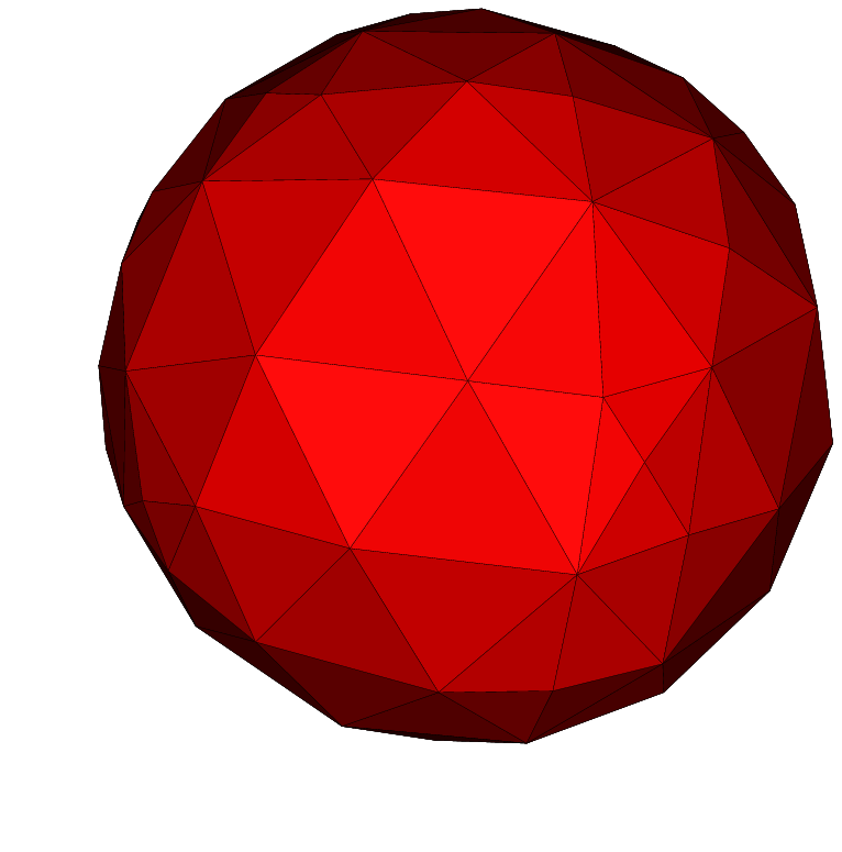
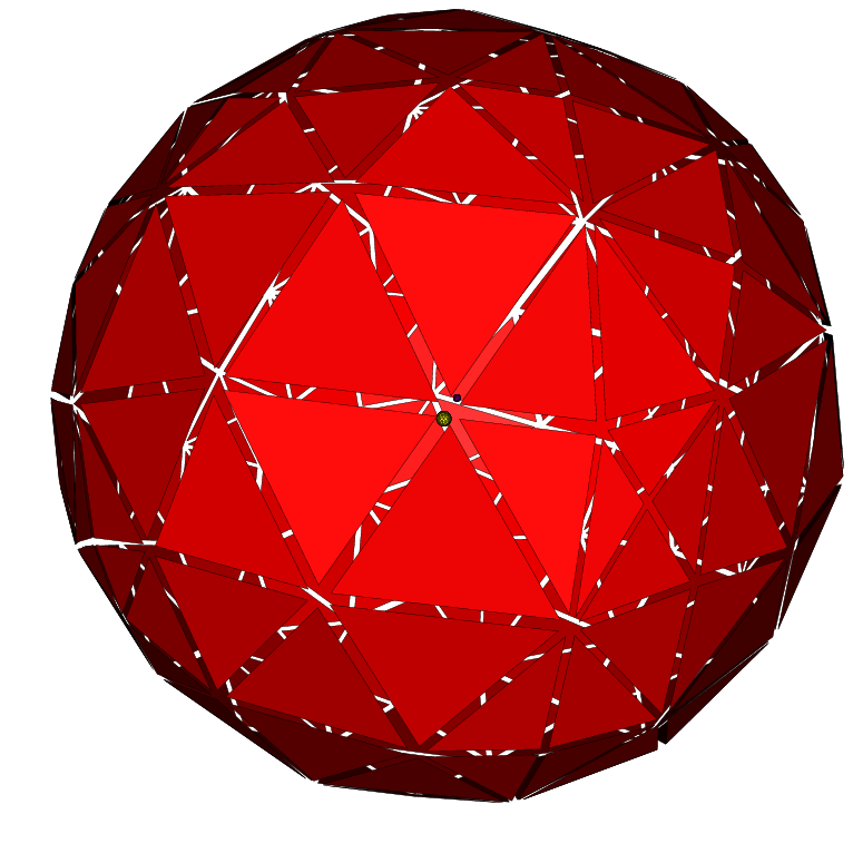
Figure 6. The coarse binary black hole mesh (approximately 6,000 vertices and 31,000 simplices).

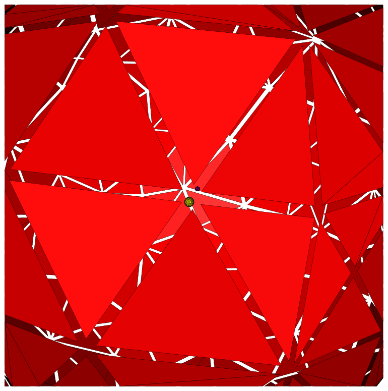
Figure 7. Exploded view of the coarse binary black hole mesh showing the two interior hole boundaries.

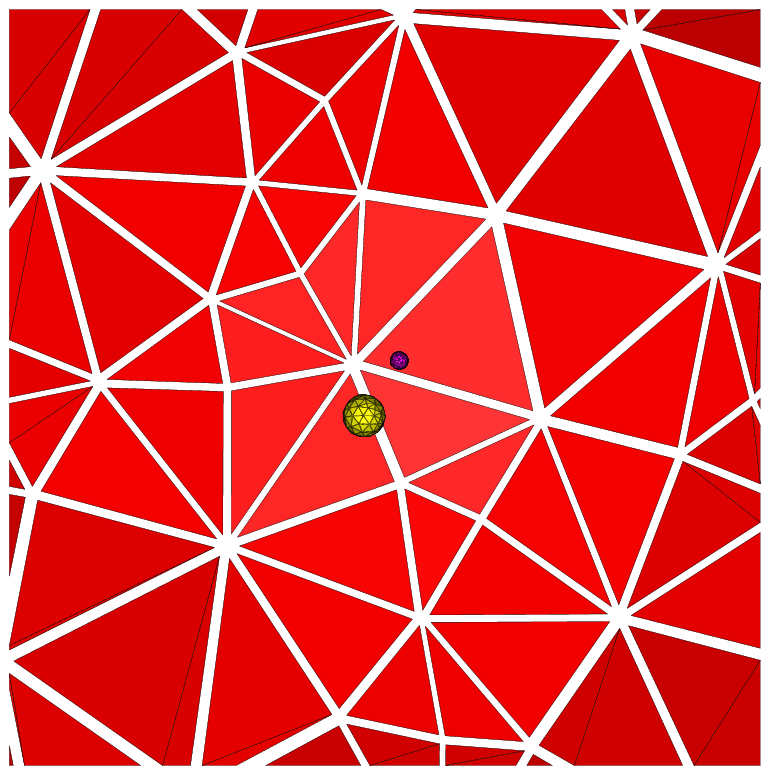
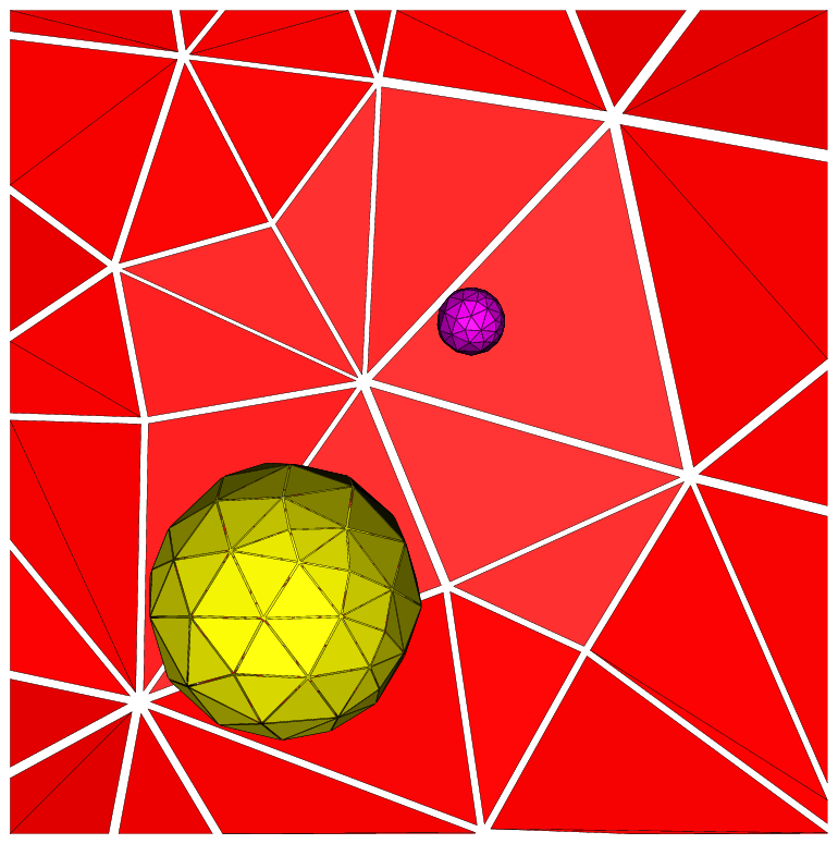
Figure 8. Closeup of the interior of the coarse binary black hole mesh. The interior holes surfaces of black hole coarse mesh; the larger hole surface is colored yellow, the smaller hole surface is colored purple, and the exterior boundary is colored red.

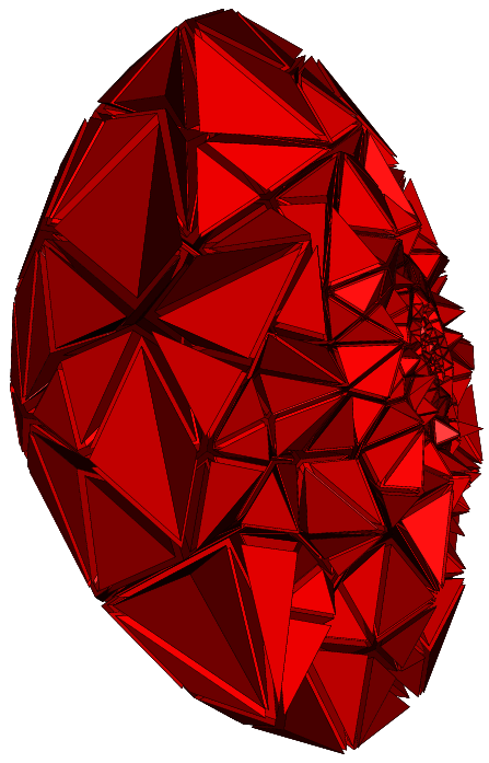
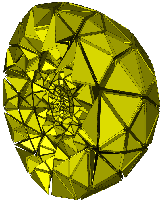
Figure 9. Subdomains 2 (red) and 4 (yellow) from spectral bisection of the coarse binary black hole mesh; these subdomains enclose two smaller subdomains that contain the inner holes.

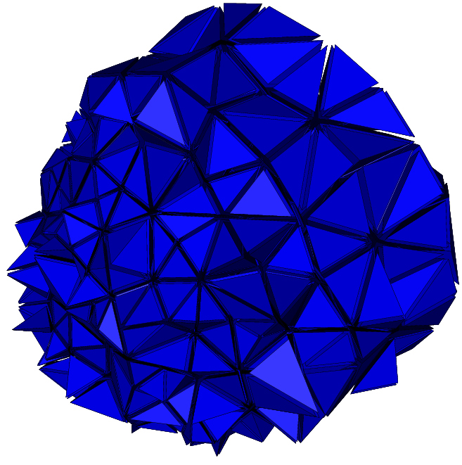
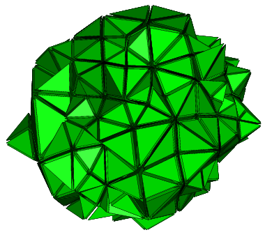
Figure 10. Subdomains 3 (blue) and 1 (green) from spectral bisection of the coarse binary black hole mesh; these subdomains each contain one of the inner holes.

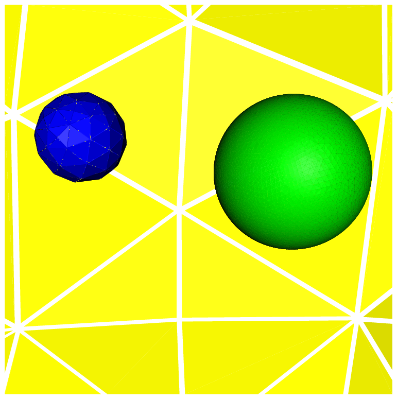
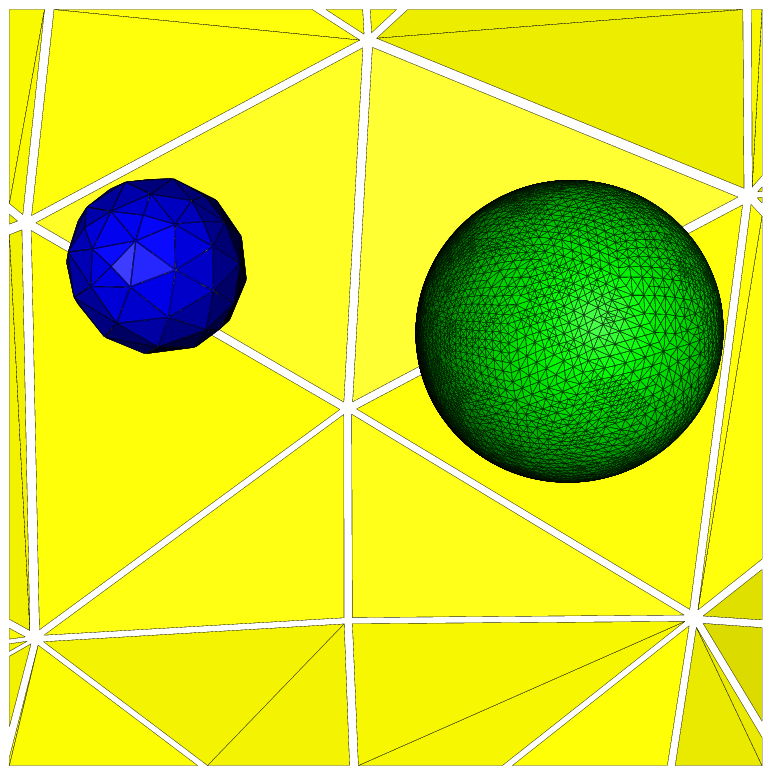
Figure 11. Closeup of the subdomain 1 refined mesh around the surface of the smaller hole. (Approximately 51,000 vertices and 266,000 simplices; only faces of tetrahedra on the boundary surfaces are shown).

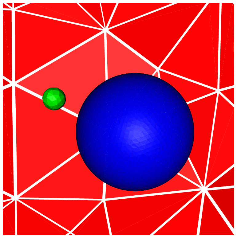
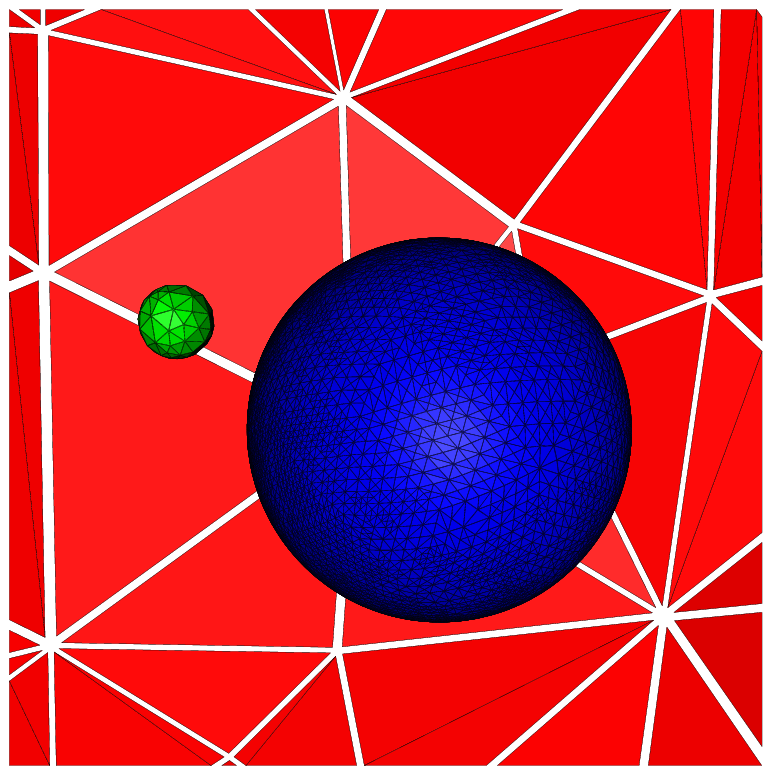
Figure 12. Closeup of the subdomain 3 refined mesh around the surface of the larger hole. (Approximately 45,000 vertices and 228,000 simplices; only faces of tetrahedra on the boundary surfaces are show).

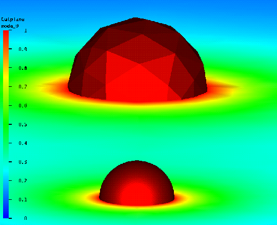
Figure 13. The conformal factor $\phi$ from the adapted subdomain 1 solve.

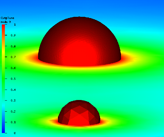
Figure 14. The conformal factor $\phi$ from the adapted subdomain 3 solve.

5. Summary

In this paper we considered the design of adaptive multilevel finite element methods for certain elliptic systems arising in geometric analysis and general relativity. We began with a brief introduction to nonlinear elliptic tensor systems on manifolds, and then discussed adaptive finite element methods for this class of problems. We derived two a posteriori error indicators, one of which was local residual-based, and one of which was based on a global linearized adjoint or dual problem.

The implementation of these methods and indicators in the ANSI C finite element software package MC was discussed, including detailed descriptions of some of the more interesting algorithms and data structures it employs. MC was designed by the author specifically for solving general second-order nonlinear elliptic systems of tensor equations on Riemannian manifolds with boundary, including domains requiring multiple coordinate systems. The key feature of MC which makes it particularly useful for highly complex tensor systems of PDEs arising in geometric analysis and general relativity is its abstraction; in addition to the support for multi-chart manifolds, the MC user supplies only two ANSI C functions representing the weak form of the tensor system $\langle F(u),v\rangle$ along with its linearization form $\langle DF(u)w,v\rangle$. Moreover, the forms themselves may be implemented almost exactly as they are written on paper, due to the fact that the quadrature-based assembly allows for tensor expressions to be treated discretely as point tensors rather than tensor fields. If residual-based or duality-based a posteriori error estimation is to be used, then the user must provide a third function $F(u)$, which is essentially the strong form of the differential equation as needed for the residual and duality indicators given in Section 2.3. We also described an unusual approach taken in MC for using parallel computers in an adaptive setting, based on joint work with R. Bank [9]. We then derived global $L^{2}$- and $H^{1}$-error estimates for the solutions produced by the parallel algorithm, by interpreting the algorithm as a special partition of unity method [5] and by using the recent local estimates of Xu and Zhou [97].

As an illustrative example, we took a brief look at the Hamiltonian and momentum constraints in the Einstein equations. We first summarized a number of operator properties and solvability results recently established in [56], and then derived two a priori error estimates for Galerkin approximations, completing the theoretical framework for effective use of adaptive multilevel finite element methods. We finished by presenting an illustrative example using the MC software. More detailed examples may be found in [55, 26].

References

- [1] R. A. Adams. Sobolev Spaces. Academic Press, San Diego, CA, 1978.
- [2] B. Aksoylu. Adaptive Multilevel Numerical Methods. PhD thesis, Department of Mathematics, UC San Diego, 2001.
- [3] D.N. Arnold, A. Mukherjee, and L. Pouly. Locally adapted tetrahedral meshes using bisection. SIAM J. Sci. Statist. Comput., 22(2):431–448, 1997.
- [4] T. Aubin. Nonlinear Analysis on Manifolds. Monge-Ampére Equations. Springer-Verlag, New York, NY, 1982.
- [5] I. Babuška and J. M. Melenk. The partition of unity finite element method. Internat. J. Numer. Methods Engrg., 40:727–758, 1997.
- [6] I. Babuška and W.C. Rheinboldt. Error estimates for adaptive finite element computations. SIAM J. Numer. Anal., 15:736–754, 1978.
- [7] I. Babuška and W.C. Rheinboldt. A posteriori error estimates for the finite element method. Int. J. Numer. Meth. Engrg., 12:1597–1615, 1978.
- [8] N. Baker, M. Holst, and F. Wang. Adaptive multilevel finite element solution of the Poisson-Boltzmann equation II: refinement at solvent accessible surfaces in biomolecular systems. J. Comput. Chem., 21:1343–1352, 2000.
- [9] R. Bank and M. Holst. A new paradigm for parallel adaptive mesh refinement. SIAM J. Sci. Comput., 22(4):1411–1443, 2000.
- [10] R. E. Bank. PLTMG: A Software Package for Solving Elliptic Partial Differential Equations, Users’ Guide 8.0. Software, Environments and Tools, Vol. 5. SIAM, Philadelphia, PA, 1998.
- [11] R. E. Bank and T. F. Dupont. An optimal order process for solving finite element equations. Math. Comp., 36(153):35–51, 1981.
- [12] R. E. Bank, T. F. Dupont, and H. Yserentant. The hierarchical basis multigrid method. Numer. Math., 52:427–458, 1988.
- [13] R. E. Bank, M. Holst, B. Mantel, J. Periaux, and C. H. Zhou. CFD PPLTMG: Using a posteriori error estimates and domain decomposition. In ECCOMAS 98, New York, NY, 1998. John Wiley & Sons.
- [14] R. E. Bank and H. D. Mittelmann. Stepsize selection in continuation procedures and damped Newton’s method. J. Computational and Applied Mathematics, 26:67–77, 1989.
- [15] R. E. Bank and D. J. Rose. Parameter selection for Newton-like methods applicable to nonlinear partial differential equations. SIAM J. Numer. Anal., 17(6):806–822, 1980.
- [16] R. E. Bank and D. J. Rose. Global Approximate Newton Methods. Numer. Math., 37:279–295, 1981.
- [17] R. E. Bank and D. J. Rose. Analysis of a multilevel iterative method for nonlinear finite element equations. Math. Comp., 39(160):453–465, 1982.
- [18] R. E. Bank and R. K. Smith. A posteriori error estimates based on hierarchical bases. SIAM J. Numer. Anal., 30(4):921–935, 1993.
- [19] R. E. Bank and R. K. Smith. Mesh smoothing using a posteriori error estimates. SIAM J. Numer. Anal., 34:979–997, 1997.
- [20] R. E. Bank and A. Weiser. Some a posteriori error estimators for elliptic partial differential equations. Math. Comp., 44(170):283–301, 1985.
- [21] E. Bänsch. An adaptive finite-element strategy for the three-dimsional time-dependent Navier-Stokes equations. Journal of Computional and Applied Mathematics, 36:3–28, 1991.
- [22] E. Bänsch. Local mesh refinement in 2 and 3 dimensions. Impact of Computing in Science and Engineering, 3:181–191, 1991.
- [23] E. Bänsch and K. G. Siebert. A posteriori error estimation for nonlinear problems by duality techniques. Technical report, Institut für Angewandte Mathematik, Hermann-Herder-Strase 10, 79104 Freiburg, Germany, 1995.
- [24] P. Bastian, K. Birken, K. Johannsen, S. Lang, N. Neuss, H. Rentz-Reichert, and C. Wieners. UG – A Flexible Software Toolbox for Solving Partial Differential Equations, 1998.
- [25] R. Beck, B. Erdmann, and R. Roitzsch. KASKADE 3.0: An ojbect-oriented adaptive finite element code. Technical Report TR95–4, Konrad-Zuse-Zentrum for Informationstechnik, Berlin, 1995.
- [26] D. Bernstein and M. Holst. Adaptive Finite Element Solution of the Constraint Equations in General Relativity II. Examples. In preparation.
- [27] J. Bey. Adaptive grid manager: AGM3D manual. Technical Report 50, SFB 382, Math. Inst. Univ. Tubingen, 1996.
- [28] S. C. Brenner and L. R. Scott. The Mathematical Theory of Finite Element Methods. Springer-Verlag, New York, NY, 1994.
- [29] F. Brezzi. Mathematical theory of finite elements. In A. K. Noor and W. D. Pilkey, editors, State-of-the-art Surveys on Finite Element Technology, pages 1–25, New York, NY, 1985. The American Society of Mechanical Engineers.
- [30] F. Brezzi, W. W. Hager, and P. A. Raviart. Error estimates for the finite element solution of variational inequalities. Numer. Math., 28:431–443, 1977.
- [31] T. F. Chan, B. Smith, and J. Zou. Overlapping Schwarz methods on unstructured meshes using non-matching coarse grids. Technical Report CAM 94-8, Department of Mathematics, UCLA, 1994.
- [32] T.F. Chan, S. Go, and L. Zikatanov. Lecture notes on multilevel methods for elliptic problems on unstructured meshes. Technical report, Dept. of Mathematics, UCLA, 1997.
- [33] Y. Choquet-Bruhat, J. Isenberg, and V. Moncrief. Solutions of constraints for Einstein equations. C.R. Acad. Sci. Paris, 315:349–355, 1992.
- [34] Y. Choquet-Bruhat and J. W. York, Jr. The Cauchy problem. In A. Held, editor, General Relativity and Gravitation, New York, 1980. Plenum Press.
- [35] P. G. Ciarlet. The Finite Element Method for Elliptic Problems. North-Holland, New York, NY, 1978.
- [36] Ph. Clément. Approximation by finite element functions using local regularization. R.A.I.R.O., 2:77–84, 1975.
- [37] W. Dahmen. Smooth piecewise quadratic surfaces. Mathematical Methods in Computer-Aided Geometric Design, pages 181–193, 1989.
- [38] W. Dahmen and C. Micchelli. Subdivision algorithms for the generation of box spline surfaces. Computer-Aided Geometric Design, 18(2):115–129, 1984.
- [39] P. J. Davis. Interpolation and Approximation. Dover Publications, Inc., New York, NY, 1963.
- [40] R. S. Dembo, S. C. Eisenstat, and T. Steihaug. Inexact Newton Methods. SIAM J. Numer. Anal., 19(2):400–408, 1982.
- [41] R. A. DeVore and G. G. Lorentz. Constructive Approximation. Springer-Verlag, New York, NY, 1993.
- [42] S. C. Eisenstat and H. F. Walker. Globally Convergent Inexact Newton Methods. Technical report, Dept. of Mathematics and Statistics, Utah State University, 1992.
- [43] D. Estep, M. Holst, and D. Mikulencak. Accounting for stability: a posteriori error estimates for finite element methods based on residuals and variational analysis. Communications in Numerical Methods in Engineering, 18(1):15–30, 2002.
- [44] R. Falk. Error estimates for the approximation of a class of variational inequalities. Math. Comput., 28:963–971, 1974.
- [45] S. Fucik and A. Kufner. Nonlinear Differential Equations. Elsevier Scientific Publishing Company, New York, NY, 1980.
- [46] M. Griebel and M. A. Schweitzer. A particle-partition of unity method for the solution of elliptic, parabolic, and hyperbolic PDEs. SIAM J. Sci. Statist. Comput., 22(3):853–890, 2000.
- [47] C.M. Grimm. Modeling Surfaces of Arbitrary Topology using Manifolds. PhD thesis, Department of Computer Science, Brown University, May 1996.
- [48] C.M. Grimm and J.F. Hughes. Modeling surfaces of arbitrary topology using manifolds. In Graphics (Proceedings of SIGGRAPH ’95), volume 29(4) of SIGGRAPH, pages 359–369. ACM, July, 1995.
- [49] W. Hackbusch. Multi-grid Methods and Applications. Springer-Verlag, Berlin, Germany, 1985.
- [50] W. Hackbusch. Iterative Solution of Large Sparse Systems of Equations. Springer-Verlag, Berlin, Germany, 1994.
- [51] S. W. Hawking and G. F. R. Ellis. The Large Scale Structure of Space-Time. Cambridge University Press, Cambridge, MA, 1973.
- [52] E. Hebey. Sobolev Spaces on Riemannian Manifolds. Springer-Verlag, Berlin, Germany, 1991.
- [53] M. Holst. Finite element approximation theory on Riemannian manifolds. In preparation.
- [54] M. Holst, N. Baker, and F. Wang. Adaptive multilevel finite element solution of the Poisson-Boltzmann equation I: algorithms and examples. J. Comput. Chem., 21:1319–1342, 2000.
- [55] M. Holst and D. Bernstein. Adaptive Finite Element Solution of the Constraint Equations in General Relativity I. Algorithms. In preparation.
- [56] M. Holst and D. Bernstein. Weak solutions to the Einstein constraint equations on manifolds with boundary. In preparation.
- [57] M. Holst and E. Titi. Determining projections and functionals for weak solutions of the Navier-Stokes equations. In Yair Censor and Simeon Reich, editors, Recent Developments in Optimization Theory and Nonlinear Analysis, volume 204 of Contemporary Mathematics, Providence, Rhode Island, 1997. American Mathematical Society.
- [58] M. Holst and S. Vandewalle. Schwarz methods: to symmetrize or not to symmetrize. SIAM J. Numer. Anal., 34(2):699–722, 1997.
- [59] J. Isenberg. Constant mean curvature solutions of the Einstein constraint equations on closed manifolds. Classical and Quantum Gravity, 12:2249–2274, 1995.
- [60] J. Isenberg and V. Moncrief. A set of nonconstant mean curvature solutions of the Einstein constraint equations on closed manifolds. Classical and Quantum Gravity, 13:1819–1847, 1996.
- [61] J. W. Jerome and T. Kerkhoven. A finite element approximation theory for the drift diffusion semiconductor model. SIAM J. Numer. Anal., 28(2):403–422, 1991.
- [62] H. B. Keller. Numerical Methods in Bifurcation Problems. Tata Institute of Fundamental Research, Bombay, India, 1987.
- [63] H. B. Keller. Numerical Methods for Two-Point Boundary-Value Problems. Dover Publications, New York, NY, 1992.
- [64] T. Kerkhoven and J. W. Jerome. stability of finite element approximations of elliptic gradient equations. Numer. Math., 57:561–575, 1990.
- [65] J. M. Lee. Riemannian Manifolds. Springer-Verlag, New York, NY, 1997.
- [66] A. Liu and B. Joe. Relationship between tetrahedron shape measures. BIT, 34:268–287, 1994.
- [67] A. Liu and B. Joe. Quality local refinement of tetrahedral meshes based on bisection. SIAM J. Sci. Statist. Comput., 16(6):1269–1291, 1995.
- [68] J.L. Liu and W.C. Rheinboldt. A posteriori finite element error estimators for indefinite elliptic boundary value problems. Numer. Funct. Anal. and Optimiz., 15(3):335–356, 1994.
- [69] J.L. Liu and W.C. Rheinboldt. A posteriori finite element error estimators for parametrized nonlinear boundary value problems. Numer. Funct. Anal. and Optimiz., 17(5):605–637, 1996.
- [70] J. E. Marsden and T. J. R. Hughes. Mathematical Foundations of Elasticity. Dover Publications, New York, NY, 1994.
- [71] J.M. Maubach. Local bisection refinement for N-simplicial grids generated by relection. SIAM J. Sci. Statist. Comput., 16(1):210–277, 1995.
- [72] E.P. Mucke. Shapes and Implementations in Three-Dimensional Geometry. PhD thesis, Dept. of Computer Science, University of Illinois at Urbana-Champaign, 1993.
- [73] A. Mukherjee. An Adaptive Finite Element Code for Elliptic Boundary Value Problems in Three Dimensions with Applications in Numerical Relativity. PhD thesis, Dept. of Mathematics, The Pennsylvania State University, 1996.
- [74] J. A. Nitsche and A. H. Schatz. Interior estimates for Ritz-Galerkin methods. Math. Comp., 28:937–958, 1974.
- [75] N. O’Murchadha and J.W. York, Jr. Initial-value problem of general relativity. I. General formulation and physical interpretation. Phys. Rev. D, 10(2):428–436, July, 1974.
- [76] N. O’Murchadha and J.W. York, Jr. Initial-value problem of general relativity. II. Stability of solutions of the initial-value equations. Phys. Rev. D, 10(2):437–446, July, 1974.
- [77] N. O’Murchadha and J.W. York, Jr. Existence and uniqueness of solutions of the Hamiltonian constraint of general relativity on compact manifolds. J. Math. Phys., 14(11):1551–1557, November, 1973.
- [78] J. M. Ortega and W. C. Rheinboldt. Iterative Solution of Nonlinear Equations in Several Variables. Academic Press, New York, NY, 1970.
- [79] M.C. Rivara. Algorithms for refining triangular grids suitable for adaptive and multigrid techniques. International Journal for Numerical Methods in Engineering, 20:745–756, 1984.
- [80] M.C. Rivara. Local modification of meshes for adaptive and/or multigrid finite-element methods. Journal of Computational and Applied Mathematics, 36:79–89, 1991.
- [81] I.G. Rosenberg and F. Stenger. A lower bound on the angles of triangles constructed by bisecting the longest side. Math. Comp., 29:390–395, 1975.
- [82] S. Rosenberg. The Laplacian on a Riemannian Manifold. Cambridge University Press, Cambridge, MA, 1997.
- [83] J. W. Ruge and K. Stüben. Algebraic multigrid (AMG). In S. F. McCormick, editor, Multigrid Methods, volume 3 of Frontiers in Applied Mathematics, pages 73–130. SIAM, Philadelphia, PA, 1987.
- [84] A. H. Schatz. An oberservation concerning Ritz-Galerkin methods with indefinite bilinear forms. Math. Comp., 28(128):959–962, 1974.
- [85] A. H. Schatz and J. Wang. Some new error estimates for Ritz-Galerkin methods with minimal regularity assumptions. Math. Comp., 62:445–475, 2000.
- [86] G. Schwarz. Hodge Decomposition: A Method for Solving Boundary Value Problems. Springer-Verlag, New York, NY, 1991.
- [87] L. R. Scott and S. Zhang. Finite element interpolation of nonsmooth functions satisfying boundary conditions. Math. Comp., 54(190):483–493, 1990.
- [88] M. Stynes. On faster convergence of the bisection method for all triangles. Math. Comp., 35:1195–1201, 1980.
- [89] P. Vanek, J. Mandel, and M. Brezina. Algebraic multigrid on unstructured meshes. Technical Report UCD/CCM 34, Center for Computational Mathematics, University of Colorado at Denver, 1994.
- [90] R. Verfürth. A posteriori error estimates for nonlinear problems. Finite element discretizations of elliptic equations. Math. Comp., 62(206):445–475, 1994.
- [91] R. Verfürth. A Review of A Posteriori Error Estimation and Adaptive Mesh-Refinement Techniques. John Wiley & Sons Ltd, New York, NY, 1996.
- [92] R. M. Wald. General Relativity. University of Chicago Press, Chicago, IL, 1984.
- [93] J. Wloka. Partial Differential Equations. Cambridge University Press, Cambridge, MA, 1992.
- [94] J. Xu. Iterative methods by space decomposition and subspace correction. SIAM Review, 34(4):581–613, 1992.
- [95] J. Xu. A novel two-grid method for semilinear elliptic equations. Technical report, Dept. of Mathematics, Penn State University, 1992.
- [96] J. Xu. Two-grid finite element discretization for nonlinear elliptic equations. Technical report, Dept. of Mathematics, Penn State University, 1992.
- [97] J. Xu and A. Zhou. Local and parallel finite element algorithms based on two-grid discretizations. Math. Comp., 69:881–909, 2000.
- [98] K. Yosida. Functional Analysis. Springer-Verlag, Berlin, Germany, 1980.