A Two-Dimensional Improvement for Farr-Gao Algorithm

Abstract

Farr-Gao algorithm is a state-of-the-art algorithm for reduced Gröbner bases of vanishing ideals of finite points, which has been implemented in Maple^® as a build-in command. In this paper, we present a two-dimensional improvement for it that employs a preprocessing strategy for computing reduced Gröbner bases associated with tower subsets of given point sets. Experimental results show that the preprocessed Farr-Gao algorithm is more efficient than the classical one.

Keywords: Gröbner basis; Vanishing ideal; Tower set; Gröbner éscalier; Newton interpolation basis

2000 Mathematics Subject Classification: 13P10

1 Introduction

Let $\mathbb{F}$ be a field, and let $\Pi^{d}:=\mathbb{F}[x_{1},x_{2},\ldots,x_{d}]$ denote the $d$-variate polynomial ring over $\mathbb{F}$. It is well known that the set of polynomials in $\Pi^{d}$ that vanish at a finite nonempty set $\Xi\subset\mathbb{F}^{d}$ forms an ideal in $\Pi^{d}$ which is called the vanishing ideal of $\Xi$, denoted by $\mathcal{I}(\Xi)$. In view of the applications of vanishing ideals in the fields of mathematics and other sciences in recent years[6, 8], there has been increasing interest in their Gröbner bases[1] and Gröbner éscaliers (aka standard set, standard monomials etc.)[12].

The most significant milestone of computing vanishing ideals is the Buchberger -Möller algorithm [11] that yields, for fixed $\Xi$ and monomial order $\prec$ on $\Pi^{d}$, the reduced Gröbner basis $G$ and the Gröbner éscalier $M$ of $\mathcal{I}(\Xi)$ w.r.t. $\prec$. It also produces a Newton interpolation basis $N$ for the $\mathbb{F}$-linear space spanned by $M$. One decade later, MMM algorithm in [10] extended Buchberger-Möller algorithm to solve general zero-dimensional ideals. And then, [7] introduced a modular version of Buchberger-Möller algorithm with lower complexity in $\mathbb{Q}^{d}$. All these three algorithms apply Gauss elimination on generalized Vandermonde matrices regardless of the order of the points in $\Xi$.

As is well known, $G$ depends not only on $\#\Xi$ (as in univariate cases) but significantly on the geometry (distribution) of $\Xi$ that is complex in $\mathbb{F}^{d}$ (see [14]). However, the algorithms mentioned above do not take this into account. In 2006, Farr and Gao [5] presented a more effcient algorithm for $G$ (called Farr-Gao algorithm hereafter) that has been implemented in Maple^® as build-in command VanishingIdeal. Arguably, the most distinguishing feature of Farr-Gao algorithm is its point-sorting strategy that provides the possibility to borrow the idea of univariate Newton interpolation. Once the points are sorted, the computation will be performed along parallel lines, one after another. On each line, we are essentially solving univariate Newton interpolation and hence the amount of reduction is decreased. The process of Farr-Gao algorithm implies that multivariate Newton interpolation would be helpful for the computation of vanishing ideals. Concretely, if we could theoretically obtain a Newton interpolation basis of some subset of $\Xi$, then the amount of reduction of Farr-Gao algorithm would be decreased further.

Let $\Xi$ be a Cartesian set in $\mathbb{F}^{d}$. [13] gave the unique Gröbner éscalier $M$ of $\mathcal{I}(\Xi)$ in theory which implies that $\mathcal{I}(\Xi)$ has a unique reduced Gröbner bases w.r.t. any monomial order (see [9]). Moreover, we can also construct Newton interpolation bases for $\Xi$ theoretically. Based on this, [15] proposed a bivariate preprocessing paradigm for Buchberger-Möller algorithm that inputs the monomial (Gröbner éscalier) and Newton interpolation basis for a maximal Cartesian subset of $\Xi$ into Buchberger-Möller algorithm as initial values. However, since the distribution of a Cartesian set is fairly restricted, in many cases the maximal Cartesian subsets are not large enough and therefore the improvement is minor.

In the following, we first introduce a new type of finite nonempty sets, tower sets, in $\mathbb{F}^{2}$ that have “freer” distributions than bivariate Cartesian sets whose formal definition is provided in Section 2 where we also establish a new criterion for bivariate Cartesian sets for the purpose of investigating the relation between tower sets and Cartesian sets. Next, in Section 3, we theoretically offer the Gröbner éscaliers of vanishing ideals of tower sets w.r.t. commonly used monomial orders as well as the Newton interpolation bases spanned by them. And, finally, these results lead to our main algorithm and the timings of some experiments are given.

2 Bivariate tower sets

Let $\mathbb{N}_{0}$ stand for the monoid of nonnegative integers. A polynomial $f\in\Pi^{2}=\mathbb{F}[x,y]$ is of the form

$$f=\sum_{(i,j)\in\mathbb{N}_{0}^{2}}c_{ij}x^{i}y^{j},\hskip 22.76228pt\#\{(i,j)\in\mathbb{N}_{0}^{2}:0\neq c_{ij}\in\mathbb{F}\}<\infty,$$

where monomial $x^{i}y^{j}$ is a product for vector $(i,j)$. The set of all monomials in $\Pi^{2}$ is denoted by $\mathbb{T}^{2}$.

Fix a monomial order $\prec$ on $\Pi^{2}$ that could be lexicographical order $\prec_{\text{lex}}$ (plex(x, y) in Maple^®), inverse lexicographical order $\prec_{\text{inlex}}$ (plex(y, x) in Maple^®), graded lexicographical order $\prec_{\text{grlex}}$ (grlex(x, y) in Maple^®), or graded reverse lexicographical order $\prec_{\text{grevlex}}$ (tdeg(x, y) in Maple^®) etc, cf. [1]. For all nonzero $f\in\Pi^{2}$, we let $\mathrm{LT}_{\prec}(f)$ signify the leading term, $\mathrm{LM}_{\prec}(f)$ the leading monomial, and $\mathrm{LC}_{\prec}(f)$ the leading coefficient of $f$. Furthermore, for a nonempty set $F\subset\Pi^{2}$, set

$$\mathrm{LM}_{\prec}(F):=\{\mathrm{LM}_{\prec}(f):f\in F\}.$$

Let $G$ be the reduced Gröbner basis for a zero-dimensional ideal $\mathcal{I}\subset\Pi^{2}$ w.r.t. $\prec$. According to [12], the monomial set

$$\mathcal{N}_{\prec}(\mathcal{I}):=\{t\in\mathbb{T}^{2}:\mathrm{LM}_{\prec}(g)\nmid t,\forall g\in G\}$$ (1)

forms the Gröbner éscalier of $\mathcal{I}$ w.r.t. $\prec$, and its corner

$$\mathcal{C}[\mathcal{N}_{\prec}(\mathcal{I})]:=\left\{t\in\mathbb{T}^{2}:x|t\Rightarrow t/x\in\mathcal{N}_{\prec}(\mathcal{I}),y|t\Rightarrow t/y\in\mathcal{N}_{\prec}(\mathcal{I})\right\}\backslash\mathcal{N}_{\prec}(\mathcal{I})$$ (2)

is equal to $\mathrm{LM}_{\prec}(G)$.

Let $\mathcal{A}$ be a finite nonempty set in $\mathbb{N}_{0}^{2}$. It is called lower if for any $(i,j)\in\mathcal{A}$ we always have

$$\{(i^{\prime},j^{\prime})\in\mathbb{N}_{0}^{2}:0\leq i^{\prime}\leq i,0\leq j^{\prime}\leq j\}\subseteq\mathcal{A}.$$ (3)

Set

$$\mathrm{b}_{x}(\mathcal{A}):=\max_{(i,0)\in\mathcal{A}}i,\qquad\mathrm{b}_{y}(\mathcal{A}):=\max_{(0,j)\in\mathcal{A}}j.$$ (4)

Subfigure (b) of Fig. 1 illustrates a lower set with $(\mathrm{b}_{x},\mathrm{b}_{y})=(4,7)$ labeled. Obviously, $\mathrm{b}_{x}(\mathcal{A})$ and $\mathrm{b}_{y}(\mathcal{A})$ alone are not enough to determine $\mathcal{A}$. Hence, we introduce sequences $m_{0},m_{1},\ldots,m_{\mathrm{b}_{y}(\mathcal{A})}$ and $n_{0},n_{1},\ldots,n_{\mathrm{b}_{x}(\mathcal{A})}$ that can uniquely determine $\mathcal{A}$ respectively, where

$$m_{j}= \max_{(i,j)\in\mathcal{A}}i,\quad 0\leq j\leq\mathrm{b}_{y}(\mathcal{A}),$$

$$n_{i}= \max_{(i,j)\in\mathcal{A}}j,\quad 0\leq i\leq\mathrm{b}_{x}(\mathcal{A}).$$

It is easy to see that (4) implies $m_{0}=\mathrm{b}_{x}(\mathcal{A})$ and $n_{0}=\mathrm{b}_{y}(\mathcal{A})$. Thus, it makes sense to write

$$\mathcal{A}=\mathrm{L}_{x}(m_{0},m_{1},\ldots,m_{\mathrm{b}_{y}(\mathcal{A})})=\mathrm{L}_{y}(n_{0},n_{1},\ldots,n_{\mathrm{b}_{x}(\mathcal{A})}).$$ (5)

A simple observation shows that the lower set in Subfigure (b) of Fig. 1 is

$$\mathrm{L}_{x}(4,3,3,2,1,0,0,0)=\mathrm{L}_{y}(7,4,3,2,0).$$

Moreover, from (3) we can deduce that both $m_{0},\ldots,m_{\mathrm{b}_{y}(\mathcal{A})}$ and $n_{0},\ldots,n_{\mathrm{b}_{x}(\mathcal{A})}$ are monotonically decreasing sequences. Furthermore, if they are strictly monotonically decreasing, then we say that $\mathcal{A}$ is $x$-strict (resp. $y$-strict) lower.

As index sets, the lower sets in $\mathbb{N}_{0}^{2}$ are used to label Cartesian sets in $\mathbb{F}^{2}$ as follows.

Definition 2.1

[9] A finite nonempty set $\Xi\subset\mathbb{F}^{2}$ of distinct points is Cartesian if and only if there exists a lower set $\mathcal{A}\subset\mathbb{N}_{0}^{2}$ and two injective functions $\mathrm{x,y}:\mathbb{N}_{0}\rightarrow\mathbb{F}$ such that $\Xi$ can be written as

$$\Xi=\left\{\left(\mathrm{x}(i),\mathrm{y}(j)\right)\in\mathbb{F}^{2}:(i,j)\in\mathcal{A}\right\}.$$ (6)

$\Xi$ is also called $\mathcal{A}$-Cartesian.

Subfigure (a) of Fig. 1 illustrates a Cartesian set that is labelled by the lower set mentioned above.

Given a finite nonempty set $\Xi\subset\mathbb{F}^{2}$ of distinct points. Set

$$\pi_{x}(\Xi):=\{\pi_{x}(\xi):\xi\in\Xi\}\quad\mbox{ and }\quad\pi_{y}(\Xi):=\{\pi_{y}(\xi):\xi\in\Xi\}$$

as the first and the second projection maps on $\mathbb{F}^{2}$ respectively, namely

$$\pi_{x}:\mathbb{F}^{2}\rightarrow\mathbb{F}:(x,y)\mapsto x\quad\mbox{ and }\quad\pi_{y}:\mathbb{F}^{2}\rightarrow\mathbb{F}:(x,y)\mapsto y.$$

Recall the point-sorting strategy of Farr-Gao algorithm, $\Xi$ can be decomposed vertically and horizontally as

$$\Xi= \bigcup_{\bar{x}\in\pi_{x}(\Xi)}\Xi\cap\{x=\bar{x}\}=:\bigcup_{i=0}^{\#\pi_{x}(\Xi)-1}\Xi_{i}^{y}$$ (7)

$$= \bigcup_{\bar{y}\in\pi_{y}(\Xi)}\Xi\cap\{y=\bar{y}\}=:\bigcup_{j=0}^{\#\pi_{y}(\Xi)-1}\Xi_{j}^{x},$$

where $\#\Xi_{0}^{y}\geq\cdots\geq\#\Xi_{\#\pi_{x}(\Xi)-1}^{y}$ and $\#\Xi_{0}^{x}\geq\cdots\geq\#\Xi_{\#\pi_{y}(\Xi)-1}^{x}$. Subfigure (a) of Fig.1 displays the decompositions of a Cartesian set.

In [2], two particular lower sets in $\mathbb{N}_{0}^{2}$

$$S_{x}(\Xi):= \mathrm{L}_{x}(\#\Xi_{0}^{x}-1,\ldots,\#\Xi_{\#\pi_{y}(\Xi)-1}^{x}-1),$$ (8)

$$S_{y}(\Xi):= \mathrm{L}_{y}(\#\Xi_{0}^{y}-1,\ldots,\#\Xi_{\#\pi_{x}(\Xi)-1}^{y}-1)$$

are constructed from $\Xi$ (see (b) of Fig.1 for example), which reflect the distribution of $\Xi$ in certain sense, and the following criterion for Cartesian sets in $\mathbb{F}^{2}$ is offered as well.

(a) $\Xi=\bigcup_{i=0}^{4}\Xi_{i}^{y}=\bigcup_{j=0}^{7}\Xi_{j}^{x}$

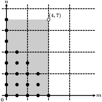
(b) $S_{y}(\Xi)$

Figure 1: Cartesian set $\Xi$, its decompositions, and $S_{y}(\Xi)$

Theorem 2.1

[2] A finite nonempty set $\Xi\subset\mathbb{F}^{2}$ is Cartesian if and only if $S_{x}(\Xi)=S_{y}(\Xi)$.

Theorem 2.1, Definition 2.1, and (8) yield the following corollary immediately.

Corollary 2.1

If a finite nonempty set $\Xi\subset\mathbb{F}^{2}$ is $\mathcal{A}$-Cartesian, then $\mathcal{A}=S_{x}(\Xi)=S_{y}(\Xi)$. Consequently, (6) can be rewritten as

$$\Xi= \left\{\left(\mathrm{x}(i),\mathrm{y}(j)\right)\in\mathbb{F}^{2}:(i,j)\in S_{x}(\Xi)\right\}$$ (9)

$$= \left\{\left(\mathrm{x}(i),\mathrm{y}(j)\right)\in\mathbb{F}^{2}:(i,j)\in S_{y}(\Xi)\right\}.$$ (10)

Unfortunately, it is difficult to extend Theorem 2.1 to three and higher dimensions. Therefore, we give the following criterion that extends to higher dimensions naturally.

Theorem 2.2

A finite nonempty set $\Xi\subset\mathbb{F}^{2}$ with decompositions (7) is Cartesian if and only if

$$\pi_{x}(\Xi_{0}^{x})\supseteq\pi_{x}(\Xi_{1}^{x})\supseteq\cdots\supseteq\pi_{x}(\Xi_{\#\pi_{y}(\Xi)-1}^{x})$$ (11)

or

$$\pi_{y}(\Xi_{0}^{y})\supseteq\pi_{y}(\Xi_{1}^{y})\supseteq\cdots\supseteq\pi_{y}(\Xi_{\#\pi_{x}(\Xi)-1}^{y}).$$ (12)

Proof:

Assume that $\Xi$ is $\mathcal{A}$-Cartesian satisfying (6) where $\mathcal{A}$ can be represented as (5) that together with (6) implies $\mathrm{b}_{y}(\mathcal{A})=\#\pi_{y}(\Xi)-1$ and

$$\pi_{x}(\Xi_{j}^{x})=\{\mathrm{x}(0),\mathrm{x}(1),\ldots,\mathrm{x}({m_{j}})\},\quad j=0,\ldots,b_{y}(\mathcal{A}).$$

Since $m_{0}\geq m_{1}\geq\cdots\geq m_{b_{y}(\mathcal{A})}\geq 0$, (11) follows. (12) can be proved in like manner.

Conversely, we suppose that (11) holds and that lower sets $S_{x}(\Xi)$ and $S_{y}(\Xi)$ have the expression (8). Then there exists a unique sequence $(n_{0},n_{1},\ldots,n_{\#\Xi_{0}^{x}-1})\in\mathbb{N}_{0}^{\#\Xi_{0}^{x}}$ such that

$$S_{x}(\Xi)=\mathrm{L}_{y}(n_{0},n_{1},\ldots,n_{\#\Xi_{0}^{x}-1})$$ (13)

where $n_{0}=\#\pi_{y}(\Xi)-1$.

Next, we shall verify that $\#\pi_{x}(\Xi)=\#\Xi_{0}^{x}$, namely we can cover $\Xi$ by exactly $\#\Xi_{0}^{x}$ vertical lines. Prove this by contradiction. It is evident from $\#\pi_{x}(\Xi)\geq\#\Xi_{0}^{x}$ that the equality fails only when $\#\pi_{x}(\Xi)>\#\Xi_{0}^{x}$, i.e., there exists at least one point $(\bar{x},\bar{y})\in\Xi$ such that $\bar{x}\notin\pi_{x}(\Xi_{0}^{x})$. However, $(\bar{x},\bar{y})\in\Xi$ simply means that there exists some $0<j\leq\#\pi_{y}(\Xi)-1$ such that $(\bar{x},\bar{y})\in\Xi_{j}^{x}$. Thus (11) implies that $\bar{x}\in\pi_{x}(\Xi_{j}^{x})\subseteq\pi_{x}(\Xi_{0}^{x})$ which contradicts $\bar{x}\notin\pi_{x}(\Xi_{0}^{x})$.

In the rest of the proof, we will use induction on $h$ to show that

$$n_{h}=\#\Xi_{h}^{y}-1,\quad h=0,\ldots,\#\pi_{x}(\Xi)-1,$$ (14)

which leads to $S_{x}(\Xi)=S_{y}(\Xi)$ immediately. When $h=0$, for every $(\bar{x},\bar{y})\in\Xi_{\#\pi_{y}(\Xi)-1}^{x}$, it follows from (11) that $\bar{x}\in\pi_{x}(\Xi_{\#\pi_{y}(\Xi)-1}^{x})\subset\pi_{x}(\Xi_{j}^{x}),0\leq j\leq\#\pi_{y}(\Xi)-2$, which means that $\#\{\Xi\cap\{x=\bar{x}\}\}\geq\#\pi_{y}(\Xi)$. But $\#\{\Xi\cap\{x=\bar{x}\}\}\leq\#\pi_{y}(\Xi)$ is trivial, we have $\#\Xi_{0}^{y}=\#\{\Xi\cap\{x=\bar{x}\}\}=\#\pi_{y}(\Xi)=n_{0}+1$, namely (14) is true for $h=0$.

Now assume (14) for $0\leq h\leq k<\#\pi_{x}(\Xi)-1$, i.e., $n_{h}=\#\Xi_{h}^{y}-1,h=0,\ldots,k$. It turns out that there exist distinct $\bar{x}_{0},\bar{x}_{1},\ldots,\bar{x}_{k}\in\pi_{x}(\Xi)$ such that $\#\{\Xi\cap\{x=\bar{x}_{h}\}\}=n_{h}+1,0\leq h\leq k$. Thus, for every $0\leq h\leq k$, $n_{h}\geq n_{k+1}$ implies $\bar{x}_{h}\in\pi_{x}(\Xi_{n_{k+1}}^{x})$. Since $(k+1,n_{k+1})\in S_{x}(\Xi)$, there exists at least one point $(\bar{x}_{k+1},\bar{y}_{k+1})\in\Xi_{n_{k+1}}^{x}$ that is not in $\Xi_{j}^{y},j=0,\ldots,k$. By (11), a similar argument leads to $\#\{\Xi\cap\{x=\bar{x}_{k+1}\}\}\geq n_{k+1}+1$ which implies $\#\Xi_{k+1}^{y}\geq n_{k+1}+1$. On the other side, it follows from induction hypothesis that every point in $\Xi_{k+1}^{y}$ belongs to some $\Xi_{j}^{x},0\leq j\leq n_{k+1}$, which implies that $\#\Xi_{k+1}^{y}\leq n_{k+1}+1$, therefore we have $\#\Xi_{k+1}^{y}=n_{k+1}+1$, namely (14) holds for $h=k+1$. Theorem 2.1 immediately implies that $\Xi$ is Cartesian.

Swapping the roles of $x$ and $y$, the other statement can be proved similarly.

$\square$

As mentioned in Section 1, [13] provides the Gröbner éscalier of the vanishing ideal of a Cartesian set in theory. In view of a later application, we restate the result only in case $d=2$.

Theorem 2.3

[13] Let $\Xi\subset\mathbb{F}^{2}$ be an $\mathcal{A}$-Cartesian set. Then Gröbner éscalier $\mathcal{N}_{\prec}(\mathcal{I}(\Xi))$ w.r.t. any monomial order $\prec$ is identical to

$$\mathfrak{M}_{\mathcal{A}}:=\{x^{i}y^{j}:(i,j)\in\mathcal{A}\}.$$ (15)

Theorem 2.3 indicates that an $\mathcal{A}$-Cartesian set in $\mathbb{F}^{2}$ has the advantage that the Gröbner éscalier of its vanishing ideal can be easily obtained from the structure of $\mathcal{A}$. Nevertheless, Theorem 2.2 illustrates that the distribution of a Cartesian set in $\mathbb{F}^{2}$ is highly restricted. Naturally, we wonder if there exists another type of finite nonempty sets with “freer” distribution and (15)-like property.

Definition 2.2

Keep the notation above. A finite nonempty set $\Xi$ in $\mathbb{F}^{2}$ is termed $x$-tower (resp. $y$-tower) if $S_{x}(\Xi)$ is $x$-strict (resp. $S_{y}(\Xi)$ is $y$-strict) and there exist two injective functions $\mathrm{x,y}:\mathbb{N}_{0}\rightarrow\mathbb{F}$ as well as $\mathrm{b}_{y}(S_{x}(\Xi))+1$ (resp. $\mathrm{b}_{x}(S_{y}(\Xi))+1$) permutations $\sigma_{0}^{x},\ldots,\sigma_{\mathrm{b}_{y}(S_{x}(\Xi))}^{x}$ (resp. $\sigma_{0}^{y},\ldots,\sigma_{\mathrm{b}_{x}(S_{y}(\Xi))}^{y}$) of set $\{0,1,\ldots,\mathrm{b}_{x}(S_{x}(\Xi))\}$ (resp. $\{0,1,\ldots,\mathrm{b}_{y}(S_{y}(\Xi))\}$) such that $\Xi$ can be written as

$$\Xi:= \{(\mathrm{x}(\sigma_{j}^{x}(i)),\mathrm{y}(j)):(i,j)\in S_{x}(\Xi)\}$$ (16)

$$\mbox{{(}resp. }\Xi:= \{(\mathrm{x}(i),\mathrm{y}(\sigma_{j}^{y}(j))):(i,j)\in S_{y}(\Xi)\}\textup{)}.$$ (17)

Fix the injective functions $\mathrm{x}$ and $\mathrm{y}$. Comparing (16) with (9), we find that if the permutations in (16) are all identical, then (16) is same as (9) in form. Assume that $(i,j)\in S_{x}(\Xi)$. If $\Xi\subset\mathbb{F}^{2}$ is Cartesian, by (9), the corresponding point of $(i,j)$ in $\Xi$ must be $(\mathrm{x}(i),\mathrm{y}(j))$. But when $\Xi$ is $x$-tower, since $\sigma_{j}^{x}$ is arbitrary, the corresponding point of $(i,j)$ could be any one of $(\mathrm{x}(h),\mathrm{y}(j)),h=0,\ldots,\mathrm{b}_{x}(S_{x}(\Xi))$. Symmetrically, a $y$-tower set has the same behavior in vertical direction. Then $\mathrm{b}_{x}(S_{x}(\Xi))=\#\Xi_{0}^{x}-1$ and $\mathrm{b}_{y}(S_{y}(\Xi))=\#\Xi_{0}^{y}-1$ lead to the following criterion for tower sets instantly.

Theorem 2.4

A finite nonempty set $\Xi\subset\mathbb{F}^{2}$ with decompositions (7) is $x$-tower (resp. $y$-tower) if and only if $S_{x}(\Xi)$ is $x$-strict (resp. $S_{y}(\Xi)$ is $y$-strict) and

$$\pi_{x}(\Xi_{0}^{x}) \supsetneq\pi_{x}(\Xi_{j}^{x}),\quad j=1,2,\ldots,\#\pi_{y}(\Xi)-1$$

$$(\mbox{resp. }\pi_{y}(\Xi_{0}^{y}) \supsetneq\pi_{y}(\Xi_{i}^{y}),\quad i=1,2,\ldots,\#\pi_{x}(\Xi)-1).$$

Subfigure (a) of Fig. 2 illustrates an $x$-tower set $\Xi$ with lower set $S_{x}(\Xi)=(11,8,6,3,1,0)$. It is easy to check that the conditions in Theorem 2.4 are satisfied.

Comparing Theorem 2.4 with Theorem 2.2, we find that in horizontal (resp. vertical) direction the distribution of an $x$-tower (resp. $y$-tower) set is “freer” than a Cartesian set. Nonetheless, when it comes to the number of the points on each line, Cartesian sets are winners this time, because their $S_{x}(\Xi)$($=S_{y}(\Xi)$) are not restricted to be $x$-strict or $y$-strict.

By Theorem 2.2, a tower set $\Xi\subset\mathbb{F}^{2}$ becomes a Cartesian set if and only if (11) or (12) is satisfied. Conversely, it follows from Theorem 2.4 that an $\mathcal{A}$-Cartesian set $\Xi\subset\mathbb{F}^{2}$ is $x$-tower(resp. $y$-tower) if and only if $\mathcal{A}$ is $x$-strict (resp. $y$-strict). Consequently, it turns out that the notions of Cartesian set and tower set in $\mathbb{F}^{2}$ are not mutually exclusive. Nevertheless, Theorem 2.2 and 2.4 also implies that most tower sets are not Cartesian and vice versa. For example, set $\Xi$ in (a) of Fig. 2 is $x$-tower but not Cartesian while set $\Xi^{\prime}$ in (b) of Fig. 2 is Cartesian but not $x$-tower or $y$-tower.

(a) $\Xi$

(b) $\Xi^{\prime}$

Figure 2: A non-Cartesian tower set and a non-tower Cartesian set

3 Main Results

3.1 Gröbner éscalier

We need the following lemma and definition before we give Theorem 3.1 that theoretically provides the Gröbner éscalier of the vanishing ideal of an $x$-tower(resp. $y$-tower) set in $\mathbb{F}^{2}$ w.r.t. $\prec_{\mathrm{grlex}}$ (resp. $\prec_{\mathrm{grevlex}}$).

Lemma 3.1

[4] Let $\Xi=\{(x_{0},y_{0}),(x_{1},y_{0}),\ldots,(x_{m},y_{0})\}\subset\mathbb{F}^{2}$ be a set of $m+1$ distinct points on line $y=y_{0}$. Then

$$\mathcal{I}(\Xi)=\langle(x-x_{0})(x-x_{1})\cdots(x-x_{m}),y-y_{0}\rangle.$$

Definition 3.1

[1] Fix a monomial order $\prec$ and let $F=\{f_{1},\ldots,f_{s}\}\subset\Pi^{d}$ with $f_{i}\neq 0$. Given $f,f^{\prime}\in\Pi^{d}$, we say that $f$ reduces to $f^{\prime}$ modulo $f_{1}$ in one step, written

$$f\xrightarrow{f_{1}}f^{\prime}$$

if and only if $\mathrm{LT}_{\prec}(f_{1})$ divides a nonzero term $\mathrm{t}$ that appears in $f$ and

$$f^{\prime}=f-\frac{\mathrm{t}}{\mathrm{LT}_{\prec}(f_{1})}f_{1}.$$

Moreover, we say that $f$ reduces to $f^{\prime}$ modulo $F$, denoted

$$f\xrightarrow{F}_{+}f^{\prime},$$

if and only if there exist a sequence of indices $i_{1},\ldots,i_{t}\in\{1,\ldots,s\}$ and a sequence of polynomials $h_{1},\ldots,h_{t-1}\in\Pi^{d}$ such that

$$f\xrightarrow{f_{i_{1}}}h_{1}\xrightarrow{f_{i_{2}}}h_{2}\xrightarrow{f_{i_{3}}}\cdots\xrightarrow{f_{i_{t-1}}}h_{t-1}\xrightarrow{f_{i_{t}}}f^{\prime}.$$

Theorem 3.1

Given an $x$-tower(resp. $y$-tower) set $\Xi\subset\mathbb{F}^{2}$. The Gröbner éscalier of vanishing ideal $\mathcal{I}(\Xi)$ w.r.t. $\prec_{\mathrm{grlex}}$ (resp. $\prec_{\mathrm{grevlex}}$) is $\mathfrak{M}_{S_{x}(\Xi)}$ (resp. $\mathfrak{M}_{S_{y}(\Xi)}$).

Proof:

We only offer the proof of the first statement. The second one can be verified in very like fashion.

Retain all the notation established previously. Fix monomial order as $\prec_{\mathrm{grlex}}$, and for simplicity the symbol will be omitted in the rest of the proof where no confusion arises. Suppose that $x$-tower set $\Xi$ has the decompositions (7). For convenience, we set $m_{j}:=\#\Xi_{j}^{x}-1,j=0,\ldots,\nu$, where $\nu=\#\pi_{y}(\Xi)-1=\mathrm{b}_{y}(S_{x}(\Xi))$. Thus, (8) implies $S_{x}(\Xi)=\mathrm{L}_{x}(m_{0},m_{1},\ldots,m_{\nu})$. Fix $0\leq j\leq\nu$. By Lemma 3.1, the ideal

$$\mathcal{I}_{j}:=\mathcal{I}(\Xi_{j}^{x})= \mathcal{I}(\{(\mathrm{x}(\sigma_{j}^{x}(i)),\mathrm{y}(j)):(i,j)\in S_{x}(\Xi)\})$$

$$= \left\langle\prod_{(i,j)\in S_{x}(\Xi)}(x-\mathrm{x}(\sigma_{j}^{x}(i))),y-\mathrm{y}(j)\right\rangle.$$

Obviously, $\mathcal{I}_{j}$’s are pairwise comaximal. Hence

$$\mathcal{I}(\Xi)=\bigcap_{j=0}^{\nu}\mathcal{I}_{j}=\prod_{j=0}^{\nu}\mathcal{I}_{j}=\prod_{j=0}^{\nu}\left\langle\prod_{(i,j)\in S_{x}(\Xi)}(x-\mathrm{x}(\sigma_{j}^{x}(i))),y-\mathrm{y}(j)\right\rangle.$$

Let $G_{N}$ be the reduced Gröbner basis for ideal $\prod_{j=0}^{N}\mathcal{I}_{j}$ w.r.t. $\prec_{\mathrm{grlex}}$, $0\leq N\leq\nu$. We will use induction on $N$ to prove

$$\mathrm{LM}(G_{N})=\{x^{m_{0}+1},x^{m_{1}+1}y,\ldots,x^{m_{N}+1}y^{N},y^{N+1}\},\quad N=0,1,\ldots,\nu.$$ (18)

First of all,

$$\mathrm{LM}\left(\prod_{(i,0)\in S_{x}(\Xi)}(x-\mathrm{x}(\sigma_{0}^{x}(i)))\right)=x^{\#\Xi_{0}^{x}}=x^{m_{0}+1}$$

leads to (18) immediately for $N=0$.

It follows from Theorem 2.4 that $m_{0}>m_{1}$ and $\pi_{x}(\Xi_{1}^{x})\subsetneq\pi_{x}(\Xi_{0}^{x})$. Therefore, we have

$$\mathcal{I}_{0}\cdot\mathcal{I}_{1}$$

$$= \left\langle\prod_{(i,0)\in S_{x}(\Xi)}(x-\mathrm{x}(\sigma_{0}^{x}(i))),y-\mathrm{y}(0)\right\rangle\cdot\left\langle\prod_{(i,1)\in S_{x}(\Xi)}(x-\mathrm{x}(\sigma_{1}^{x}(i))),y-\mathrm{y}(1)\right\rangle$$

$$= \Bigg{\langle}\prod_{(i,0)\in S_{x}(\Xi)}(x-\mathrm{x}(\sigma_{0}^{x}(i))),\Bigg{(}\prod_{(i,0)\in S_{x}(\Xi)}(x-\mathrm{x}(\sigma_{0}^{x}(i)))\Bigg{)}(y-\mathrm{y}(1)),$$

$$\phantom{\Bigg{\langle}}\Bigg{(}\prod_{(i,1)\in S_{x}(\Xi)}(x-\mathrm{x}(\sigma_{1}^{x}(i)))\Bigg{)}(y-\mathrm{y}(0)),\prod_{j=0}^{1}(y-\mathrm{y}(j))\Bigg{\rangle}$$

$$= \Bigg{\langle}\prod_{(i,0)\in S_{x}(\Xi)}(x-\mathrm{x}(\sigma_{0}^{x}(i))),\Bigg{(}\prod_{(i,1)\in S_{x}(\Xi)}(x-\mathrm{x}(\sigma_{1}^{x}(i)))\Bigg{)}(y-\mathrm{y}(0)),\prod_{j=0}^{1}(y-\mathrm{y}(j))\Bigg{\rangle}$$

where the last equality holds by

$$\prod_{(i,0)\in S_{x}(\Xi)}(x-\mathrm{x}(\sigma_{0}^{x}(i)))\Bigg{|}\Bigg{(}\prod_{(i,0)\in S_{x}(\Xi)}(x-\mathrm{x}(\sigma_{0}^{x}(i)))\Bigg{)}(y-\mathrm{y}(1)).$$

Then $\mathrm{LM}(G_{1})=\{x^{m_{0}+1},x^{m_{1}+1}y,y^{2}\}$ follows which means that (18) holds for $N=1$.

Similarly, by $m_{1}>m_{2}$ and $\pi_{x}(\Xi_{2}^{x})\subsetneq\pi_{x}(\Xi_{0}^{x})$, we obtain, after some easy computations,

$$\mathcal{I}_{0}\cdot\mathcal{I}_{1}\cdot\mathcal{I}_{2}$$

$$= \Bigg{\langle}\prod_{(i,0)\in S_{x}(\Xi)}(x-\mathrm{x}(\sigma_{0}^{x}(i))),\prod_{j=0}^{2}(y-\mathrm{y}(j)),$$

$$\phantom{\Bigg{\langle}}\Bigg{(}\prod_{(i,1)\in S_{x}(\Xi)}(x-\mathrm{x}(\sigma_{1}^{x}(i)))\Bigg{)}\Bigg{(}\prod_{(i,2)\in S_{x}(\Xi)}(x-\mathrm{x}(\sigma_{2}^{x}(i)))\Bigg{)}(y-\mathrm{y}(0)),$$

$$\phantom{\Bigg{\langle}}\Bigg{(}\prod_{(i,1)\in S_{x}(\Xi)}(x-\mathrm{x}(\sigma_{1}^{x}(i)))\Bigg{)}(y-\mathrm{y}(0))(y-\mathrm{y}(2)),$$

$$\phantom{\Bigg{\langle}}\Bigg{(}\prod_{(i,2)\in S_{x}(\Xi)}(x-\mathrm{x}(\sigma_{2}^{x}(i)))\Bigg{)}\prod_{j=0}^{1}(y-\mathrm{y}(j))\Bigg{\rangle}$$

$$=: \left\langle g_{0}^{(2)},g_{1}^{(2)},g_{2}^{(2)},g_{3}^{(2)},g_{4}^{(2)}\right\rangle.$$

We let $\hat{q},\hat{r}\in\Pi^{1}$ be the quotient and the remainder of the division of $\prod_{(i,1)\in S_{x}(\Xi)}(x-\mathrm{x}(\sigma_{1}^{x}(i)))$ by $\prod_{(i,2)\in S_{x}(\Xi)}(x-\mathrm{x}(\sigma_{2}^{x}(i)))$ respectively, namely

$$\prod_{(i,1)\in S_{x}(\Xi)}(x-\mathrm{x}(\sigma_{1}^{x}(i)))=\hat{q}\Bigg{(}\prod_{(i,2)\in S_{x}(\Xi)}(x-\mathrm{x}(\sigma_{2}^{x}(i)))\Bigg{)}+\hat{r}.$$

Denote the remainder of $g_{3}^{(2)}$ w.r.t. $g_{4}^{(2)}$ by $\bar{g}_{3}^{(2)}$. One can check readily that

$$\bar{g}_{3}^{(2)}=g_{3}^{(2)}-\hat{q}g_{4}^{(2)}.$$

On the other hand,

$$g_{2}^{(2)}=\frac{1}{\mathrm{y}(1)-\mathrm{y}(2)}\Bigg{[} \Bigg{(}\prod_{(i,2)\in S_{x}(\Xi)}(x-\mathrm{x}(\sigma_{2}^{x}(i)))\Bigg{)}g_{3}^{(2)}-$$

$$\Bigg{(}\prod_{(i,1)\in S_{x}(\Xi)}(x-\mathrm{x}(\sigma_{1}^{x}(i)))\Bigg{)}g_{4}^{(2)}\Bigg{]}$$

implies $g_{2}^{(2)}\xrightarrow{\{g_{3}^{(2)},g_{4}^{(2)}\}}_{+}0$. Consequently,

$$\mathcal{I}_{0}\cdot\mathcal{I}_{1}\cdot\mathcal{I}_{2}= \left\langle\ g_{0}^{(2)},g_{1}^{(2)},\bar{g}_{3}^{(2)},g_{4}^{(2)}\right\rangle.$$

We claim that

$$G_{2}=G^{\prime}_{2}:=\left\{g_{0}^{(2)},g_{1}^{(2)},(\mathrm{y}(1)-\mathrm{y}(2))^{-1}\bar{g}_{3}^{(2)},g_{4}^{(2)}\right\},$$

where $\mathrm{y}(1)-\mathrm{y}(2)=\mathrm{LC}\left(\bar{g}_{3}^{(2)}\right)$, i.e., $(\mathrm{y}(1)-\mathrm{y}(2))^{-1}\bar{g}_{3}^{(2)}$ is monic.

In fact, if $S(f,g)$ stands for the S-polynomial of polynomials $f,g\in\Pi^{2}$, then $S\left(g_{0}^{(2)},g_{1}^{(2)}\right)\xrightarrow{G^{\prime}_{2}}_{+}0$ follows immediately because $\mathrm{LM}\left(g_{0}^{(2)}\right)$ and $\mathrm{LM}\left(g_{1}^{(2)}\right)$ are relatively prime. Observing that $\prod_{(i,2)\in S_{x}(\Xi)}(x-\mathrm{x}(\sigma_{2}^{x}(i)))$ is a factor of $\prod_{(i,0)\in S_{x}(\Xi)}(x-\mathrm{x}(\sigma_{0}^{x}(i)))$, we get

$$S\left(g_{0}^{(2)},g_{4}^{(2)}\right)$$

$$= y^{2}g_{0}^{(2)}-x^{m_{0}-m_{2}}g_{4}^{(2)}$$

$$= y^{2}g_{0}^{(2)}-x^{m_{0}-m_{2}}g_{4}^{(2)}-\Bigg{(}\prod_{j=0}^{1}(y-\mathrm{y}(j))\Bigg{)}g_{0}^{(2)}+\Bigg{(}\prod_{j=0}^{1}(y-\mathrm{y}(j))\Bigg{)}g_{0}^{(2)}$$

$$= y^{2}g_{0}^{(2)}-x^{m_{0}-m_{2}}g_{4}^{(2)}-\Bigg{(}\prod_{j=0}^{1}(y-\mathrm{y}(j))\Bigg{)}g_{0}^{(2)}+\frac{\prod_{(i,0)\in S_{x}(\Xi)}(x-\mathrm{x}(\sigma_{0}^{x}(i)))}{\prod_{(i,2)\in S_{x}(\Xi)}(x-\mathrm{x}(\sigma_{2}^{x}(i)))}g_{4}^{(2)}$$

$$= ((\mathrm{y}(0)+\mathrm{y}(1))y-\mathrm{y}(0)\mathrm{y}(1))g_{0}^{(2)}+\left(\frac{\prod_{(i,0)\in S_{x}(\Xi)}(x-\mathrm{x}(\sigma_{0}^{x}(i)))}{\prod_{(i,2)\in S_{x}(\Xi)}(x-\mathrm{x}(\sigma_{2}^{x}(i)))}-x^{m_{0}-m_{2}}\right)g_{4}^{(2)}.$$

It is easy to see that $\mathrm{LM}\left(S\left(g_{0}^{(2)},g_{4}^{(2)}\right)\right)=x^{m_{0}+1}y$. Moreover, a simple computation leads to:

$$\mathrm{LM}\left(((\mathrm{y}(0)+\mathrm{y}(1))y-\mathrm{y}(0)\mathrm{y}(1))g_{0}^{(2)}\right) =x^{m_{0}+1}y,$$

$$\mathrm{LM}\left(\left(\frac{\prod_{(i,0)\in S_{x}(\Xi)}(x-\mathrm{x}(\sigma_{0}^{x}(i)))}{\prod_{(i,2)\in S_{x}(\Xi)}(x-\mathrm{x}(\sigma_{2}^{x}(i)))}-x^{m_{0}-m_{2}}\right)g_{4}^{(2)}\right) =x^{m_{0}}y^{2},$$

therefore

$$\max_{\prec_{\mathrm{grlex}}}\Bigg{(}\mathrm{LM}\left(((\mathrm{y}(0)+\mathrm{y}(1))y-\mathrm{y}(0)\mathrm{y}(1))g_{0}^{(2)}\right),$$

$$\phantom{\max_{\prec_{\mathrm{grlex}}}\Bigg{(}}\mathrm{LM}\left(\left(\frac{\prod_{(i,0)\in S_{x}(\Xi)}(x-\mathrm{x}(\sigma_{0}^{x}(i)))}{\prod_{(i,2)\in S_{x}(\Xi)}(x-\mathrm{x}(\sigma_{2}^{x}(i)))}-x^{m_{0}-m_{2}}\right)g_{4}^{(2)}\right)\Bigg{)}$$

$$= x^{m_{0}+1}y=\mathrm{LM}\left(S\left(g_{0}^{(2)},g_{4}^{(2)}\right)\right)$$

implies $S\left(g_{0}^{(2)},g_{4}^{(2)}\right)\xrightarrow{G_{2}^{\prime}}_{+}0$. Similarly,

$$S\left(g_{1}^{(2)},g_{4}^{(2)}\right)=\Bigg{(}x^{m_{2}+1}-\prod_{(i,2)\in S_{x}(\Xi)}(x-\mathrm{x}(\sigma_{2}^{x}(i)))\Bigg{)}g_{1}^{(2)}-\mathrm{y}(2)g_{4}^{(2)}$$

and $\mathrm{LM}\left(S\left(g_{1}^{(2)},g_{4}^{(2)}\right)\right)=x^{m_{2}+1}y^{2}$ imply

$$\max_{\prec_{\mathrm{grlex}}}\Bigg{(}\mathrm{LM}\Bigg{(}\Bigg{(}x^{m_{2}+1}-\prod_{(i,2)\in S_{x}(\Xi)}(x-\mathrm{x}(\sigma_{2}^{x}(i)))\Bigg{)}g_{1}^{(2)}\Bigg{)},\mathrm{LM}\left(-\mathrm{y}(2)g_{4}^{(2)}\right)\Bigg{)}$$

$$= \max_{\prec_{\mathrm{grlex}}}\left(x^{m_{2}}y^{3},x^{m_{2}+1}y^{2}\right)=x^{m_{2}+1}y^{2}=\mathrm{LM}\left(S\left(g_{1}^{(2)},g_{4}^{(2)}\right)\right),$$

which means that $S\left(g_{1}^{(2)},g_{4}^{(2)}\right)\xrightarrow{G_{2}^{\prime}}_{+}0$.

In like manner, we can also show that

$$S\left(g_{0}^{(2)},(\mathrm{y}(1)-\mathrm{y}(2))^{-1}\bar{g}_{3}^{(2)}\right)\xrightarrow{G_{2}^{\prime}}_{+}0,\quad S\left(g_{1}^{(2)},(\mathrm{y}(1)-\mathrm{y}(2))^{-1}\bar{g}_{3}^{(2)}\right)\xrightarrow{G_{2}^{\prime}}_{+}0.$$

Hence, there only remains $S\left((\mathrm{y}(1)-\mathrm{y}(2))^{-1}\bar{g}_{3}^{(2)},g_{4}^{(2)}\right)\xrightarrow{G_{2}^{\prime}}_{+}0$ to be verified. Actually, it can be deduced that

$$S\left((\mathrm{y}(1)-\mathrm{y}(2))^{-1}\bar{g}_{3}^{(2)},g_{4}^{(2)}\right)$$

$$= \frac{\hat{r}}{\mathrm{y}(1)-\mathrm{y}(2)}g_{1}^{(2)}+\mathrm{y}(1)\cdot(\mathrm{y}(1)-\mathrm{y}(2))^{-1}\bar{g}_{3}^{(2)}+\left(\hat{q}-x^{m_{1}-m_{2}}\right)g_{4}^{(2)}$$

whose leading monomial is $x^{m_{1}+1}y$. Thus

$$\mathrm{LM}\left(\frac{\hat{r}}{\mathrm{y}(1)-\mathrm{y}(2)}g_{1}^{(2)}\right) =x^{m_{2}}y^{3},$$

$$\mathrm{LM}\left(\mathrm{y}(1)\cdot(\mathrm{y}(1)-\mathrm{y}(2))^{-1}\bar{g}_{3}^{(2)}\right) =x^{m_{1}+1}y,$$

and

$$\mathrm{LM}\left(\left(\hat{q}-x^{m_{1}-m_{2}}\right)g_{4}^{(2)}\right)=x^{m_{1}}y^{2}$$

imply that $S\left((\mathrm{y}(1)-\mathrm{y}(2))^{-1}\bar{g}_{3}^{(2)},g_{4}^{(2)}\right)\xrightarrow{G_{2}^{\prime}}_{+}0$.

Now, these arguments lead to the conclusion that S-polynomial $S(g,g^{\prime})\xrightarrow{G^{\prime}_{2}}_{+}0$ for any two distinct $g,g^{\prime}\in G^{\prime}_{2}$. By Buchberger’s S-pair criterion, $G_{2}^{\prime}$ is a Gröbner basis for $\mathcal{I}_{0}\cdot\mathcal{I}_{1}\cdot\mathcal{I}_{2}$ w.r.t. $\prec_{\mathrm{grlex}}$. Moreover, for every $g\in G_{2}^{\prime}$, it is evident that

1. $\mathrm{LC}(g)=1$,

2. No monomial of $g$ lies in $\langle\mathrm{LT}(G_{2}^{\prime}-\{g\})\rangle$,

which means that $G_{2}^{\prime}$ is reduced, namely (18) holds for $N=2$.

Now, assume (18) for $N=k,3\leq k<\nu$. Without loss of generality, we suppose that $G_{k}=\left\{g_{0}^{(k)},\ldots,g_{k+1}^{(k)}\right\}$ with

$$\mathrm{LM}\left(g_{i}^{(k)}\right)= x^{m_{i}+1}y^{i},\quad i=0,\ldots,k,$$

$$\mathrm{LM}\left(g_{k+1}^{(k)}\right)= y^{k+1},$$

which imply that

$$g_{0}^{(k)} =\prod_{(i,0)\in S_{x}(\Xi)}(x-\mathrm{x}(\sigma_{0}^{x}(i))),$$

$$g_{k+1}^{(k)} =\prod_{j=0}^{k}(y-\mathrm{y}(j)).$$

When $N=k+1$, since $\Xi$ is $x$-tower, we obtain

$$\prod_{j=0}^{k+1}\mathcal{I}_{j}= (\prod_{j=0}^{k}\mathcal{I}_{j})\mathcal{I}_{k+1}$$

$$= \Big{\langle}g_{0}^{(k)},\ldots,g_{k+1}^{(k)}\Big{\rangle}\cdot\Bigg{\langle}\prod_{(i,k+1)\in S_{x}(\Xi)}(x-\mathrm{x}(\sigma_{k+1}^{x}(i))),y-\mathrm{y}(k+1)\Bigg{\rangle}$$

$$= \Bigg{\langle}g_{0}^{(k+1)},g_{0}^{(k)}(y-\mathrm{y}(k+1)),$$

$$\phantom{\Big{\langle}}g_{1}^{(k)}\Bigg{(}\prod_{(i,k+1)\in S_{x}(\Xi)}(x-\mathrm{x}(\sigma_{k+1}^{x}(i)))\Bigg{)},g_{1}^{(k)}(y-\mathrm{y}(k+1)),$$

$$\cdots$$

$$\phantom{\Big{\langle}}g_{k-1}^{(k)}\Bigg{(}\prod_{(i,k+1)\in S_{x}(\Xi)}(x-\mathrm{x}(\sigma_{k+1}^{x}(i)))\Bigg{)},g_{k-1}^{(k)}(y-\mathrm{y}(k+1)),$$

$$\phantom{\Big{\langle}}g_{k}^{(k)}\Bigg{(}\prod_{(i,k+1)\in S_{x}(\Xi)}(x-\mathrm{x}(\sigma_{k+1}^{x}(i)))\Bigg{)},g_{k}^{(k)}(y-\mathrm{y}(k+1)),$$

$$\phantom{\Big{\langle}}g_{k+1}^{(k)}\Bigg{(}\prod_{(i,k+1)\in S_{x}(\Xi)}(x-\mathrm{x}(\sigma_{k+1}^{x}(i)))\Bigg{)},g_{k+1}^{(k)}(y-\mathrm{y}(k+1))\Bigg{\rangle},$$

where $g_{0}^{(k+1)}=g_{0}^{(k)}$ is obvious hence $g_{0}^{(k)}(y-\mathrm{y}(k+1))$ can be removed. By the induction hypothesis, we have

$$g_{k+2}^{(k+1)}:=g_{k+1}^{(k)}(y-\mathrm{y}(k+1))=\prod_{j=0}^{k+1}(y-\mathrm{y}(j)).$$

We denote polynomial $g_{k+1}^{(k)}(\prod_{(i,k+1)\in S_{x}(\Xi)}(x-\mathrm{x}(\sigma_{k+1}^{x}(i))))$ by $g_{k+1}^{(k+1)}$. It follows from the induction hypothesis that $\mathrm{LM}\left(g_{k+1}^{(k+1)}\right)=x^{m_{k+1}+1}y^{k+1}$. Set $E_{1}:=\left\{g_{k+1}^{(k+1)}\right\}$. Suppose that $g_{k}^{(k)}(y-\mathrm{y}(k+1))\xrightarrow{E_{1}}_{+}g_{k}^{(k+1)}$. Since $m_{k}>m_{k+1}$, we have

$$\mathrm{LM}\left(g_{k}^{(k+1)}\right)=x^{m_{k}+1}y^{k}.$$

Recall case $N=2$. It is easy to see that

$$g_{k}^{(k)}\Bigg{(}\prod_{(i,k+1)\in S_{x}(\Xi)}(x-\mathrm{x}(\sigma_{k+1}^{x}(i)))\Bigg{)}\xrightarrow{F_{1}}_{+}0$$

where $F_{1}:=\left\{g_{k+1}^{(k+1)},g_{k}^{(k+1)}\right\}$, which means that $g_{k}^{(k)}(\prod_{(i,k+1)\in S_{x}(\Xi)}(x-\mathrm{x}(\sigma_{k+1}^{x}(i))))$ can be removed from the original ideal basis.

Set $E_{2}:=F_{1}$, and suppose that $g_{k-1}^{(k)}(y-\mathrm{y}(k+1))\xrightarrow{E_{2}}_{+}g_{k-1}^{(k+1)}$. We similarly deduce that $\mathrm{LM}\left(g_{k-1}^{(k+1)}\right)=x^{m_{k-1}+1}y^{k-1}$ and

$$g_{k-1}^{(k)}\Bigg{(}\prod_{(i,k+1)\in S_{x}(\Xi)}(x-\mathrm{x}(\sigma_{k+1}^{x}(i)))\Bigg{)}\xrightarrow{F_{2}}_{+}0$$

where $F_{2}:=\left\{g_{k+1}^{(k+1)},g_{k-1}^{(k+1)}\right\}$.

In this way, we construct two sequences $(E_{1},E_{2},\ldots,E_{k})$ and $(F_{1},F_{2},\ldots,F_{k})$ such that

$$g_{i}^{(k)}(y-\mathrm{y}(k+1))\xrightarrow{E_{k+1-i}}_{+} g_{i}^{(k+1)},$$

$$g_{i}^{(k)}\Bigg{(}\prod_{(i,k+1)\in S_{x}(\Xi)}(x-\mathrm{x}(\sigma_{k+1}^{x}(i)))\Bigg{)}\xrightarrow{F_{k+1-i}}_{+} 0,$$

where, for $i=1,\ldots,k$,

$$E_{i} =\left\{g_{k+2-i}^{(k+1)},\ldots,g_{k+1}^{(k+1)}\right\},$$

$$F_{i} =\left\{g_{k+1}^{(k+1)},g_{k+1-i}^{(k+1)}\right\},$$

$$\mathrm{LM}\left(g_{i}^{(k+1)}\right) =x^{m_{i}+1}y^{i}.$$

Let $\bar{g}_{i}^{(k+1)}=\mathrm{LC}\left(g_{i}^{(k+1)}\right)^{-1}g_{i}^{(k+1)},i=0,\ldots,k+2$. With similar arguments used in $N=2$ case, we can finally prove that

$$G_{k+1}=\left\{\bar{g}_{0}^{(k+1)},\bar{g}_{1}^{(k+1)},\ldots,\bar{g}_{k+2}^{(k+1)}\right\},$$

with $\mathrm{LM}\left(\bar{g}_{i}^{(k+1)}\right)=x^{m_{i}+1}y^{i},i=0,\ldots,k+1$, and $\mathrm{LM}\left(\bar{g}_{k+2}^{(k+1)}\right)=y^{k+2}$, namely (18) holds for $N=k+1$. Consequently, we have

$$\mathrm{LM}(G_{\nu})=\{x^{m_{0}+1},x^{m_{1}+1}y,\ldots,x^{m_{\nu}+1}y^{\nu},y^{\nu+1}\}.$$

Recalling (1) and (8), we have

$$\mathcal{N}(\mathcal{I}(\Xi))=\{x^{i}y^{j}:(i,j)\in S_{x}(\Xi)\}=\mathfrak{M}_{S_{x}(\Xi)},$$

which complete the proof. $\square$

3.2 Newton Basis

The $\prec\mspace{-8.0mu}-$degree of a nonzero polynomial $f\in\Pi^{2}$ (see [3]), denoted by $\delta_{\prec}(f)$, was defined to be $(i,j)\in\mathbb{N}_{0}^{2}$ satisfying

$$x^{i}y^{j}=\mathrm{LM}_{\prec}(f).$$

For every pair of polynomials $f,g\in\Pi^{2}$, if $\delta(f)\prec\delta(g)$ then we say that $f$ is of lower $\prec\mspace{-8.0mu}-$degree than $g$ and use the abbreviation

$$f\prec g:=\delta(f)\prec\delta(g).$$

In addition, $f\preceq g$ is interpreted as the $\prec\mspace{-8.0mu}-$degree of $f$ is lower than or equal to that of $g$.

Given a finite nonempty set $\Xi=\{\xi^{(0)},\xi^{(1)},\ldots,\xi^{(\mu-1)}\}\subset\mathbb{F}^{2}$. For fixed monomial order $\prec$, the Gröbner éscalier $\mathcal{N}_{\prec}(\mathcal{I}(\Xi))$ trivially forms the monomial basis for $\mu$-dimensional $\mathbb{F}$-linear space $\mathcal{P}_{\prec}(\Xi):=\mathrm{Span}_{\mathbb{F}}\mathcal{N}_{\prec}(\mathcal{I}(\Xi))\subset\Pi^{2}$ that complements $\mathcal{I}(\Xi)$, i.e.

$$\Pi^{2}=\mathcal{I}(\Xi)\oplus\mathcal{P}_{\prec}(\Xi).$$

Moreover, if subset $\{p_{0},p_{1},\ldots,p_{\mu-1}\}\subset\mathcal{P}_{\prec}(\Xi)$, with $p_{0}\prec p_{1}\prec\cdots\prec p_{\mu-1}$, satisfying

$$p_{j}(\xi^{(i)})=\delta_{ij},\quad 0\leq i\leq j\leq\mu-1,$$

then $\{p_{0},p_{1},\ldots,p_{\mu-1}\}$ is called a Newton interpolation basis for $\mathcal{P}_{\prec}(\Xi)$.

Consequently, from Theorem 3.1, $\Xi$ is $x$-tower (resp. $y$-tower) implies that $\mathcal{P}_{\prec_{\mathrm{grlex}}}(\Xi)=\mathrm{Span}_{\mathbb{F}}\mathfrak{M}_{S_{x}(\Xi)}$(resp. $\mathcal{P}_{\prec_{\mathrm{grevlex}}}(\Xi)=\mathrm{Span}_{\mathbb{F}}\mathfrak{M}_{S_{y}(\Xi)}$). The next two theorems present Newton bases for $\mathcal{P}_{\prec_{\mathrm{grlex}}}(\Xi)$ and $\mathcal{P}_{\prec_{\mathrm{grevlex}}}(\Xi)$ respectively.

Theorem 3.2

Given an $x$-tower set $\Xi\subset\mathbb{F}^{2}$ that is expressed as (16). Set polynomial

$$\phi_{ij}^{x}:=c_{ij}^{x}\prod_{t=0}^{j-1}(y-\mathrm{y}(t))\prod_{s=0}^{i-1}(x-\mathrm{x}(\sigma_{j}^{x}(s))),\quad(i,j)\in S_{x}(\Xi),$$

where

$$c_{ij}^{x}=\frac{1}{\prod_{t=0}^{j-1}(\mathrm{y}(j)-\mathrm{y}(t))\prod_{s=0}^{i-1}(\mathrm{x}(\sigma_{j}^{x}(i))-\mathrm{x}(\sigma_{j}^{x}(s)))}\in\mathbb{F}$$

and the empty products are taken as 1. Then for $(i,j),(m,n)\in S_{x}(\Xi)$ with $(i,j)\succeq_{\mathrm{inlex}}(m,n)$, we have

$$\phi_{ij}^{x}\left(\mathrm{x}(\sigma_{n}^{x}(m)),\mathrm{y}(n)\right)=\delta_{(i,j),(m,n)},$$

namely

$$\mathfrak{N}_{S_{x}(\Xi)}:=\{\phi_{ij}^{x}:(i,j)\in S_{x}(\Xi)\}$$ (19)

forms a Newton interpolation basis for $\mathcal{P}_{\prec_{\mathrm{grlex}}}(\Xi)$.

Proof:

Fix $(i,j)\in S_{x}(\Xi)$. If $(i,j)=(m,n)$, then

$$\phi_{ij}^{x}(\mathrm{x}(\sigma_{n}^{x}(m)),\mathrm{y}(n))=c_{ij}^{x}\prod_{t=0}^{j-1}(\mathrm{y}(j)-\mathrm{y}(t))\prod_{s=0}^{i-1}(\mathrm{x}(\sigma_{j}^{x}(i))-\mathrm{x}(\sigma_{j}^{x}(s)))\\ =c_{ij}^{x}/c_{ij}^{x}=1.$$

Otherwise, $(i,j)\succneqq_{\mathrm{inlex}}(m,n)$ implies $j>n$ or $j=n$ and $i>m$. When $j>n$, i.e., $j-1\geq n$, we have

$$\phi_{ij}^{x}\left(\mathrm{x}(\sigma_{n}^{x}(m)),\mathrm{y}(n)\right)=c_{ij}^{x}\prod_{t=0}^{j-1}(\mathrm{y}(n)-\mathrm{y}(t))\prod_{s=0}^{i-1}(\mathrm{x}(\sigma_{n}^{x}(m))-\mathrm{x}(\sigma_{j}^{x}(s)))=0.$$

If $j=n,i>m$, namely $i-1\geq m$, then

$$\phi_{ij}^{x}\left(\mathrm{x}(\sigma_{n}^{x}(m)),\mathrm{y}(n)\right) =c_{ij}^{x}\prod_{t=0}^{j-1}(\mathrm{y}(n)-\mathrm{y}(t))\prod_{s=0}^{i-1}(\mathrm{x}(\sigma_{n}^{x}(m))-\mathrm{x}(\sigma_{j}^{x}(s)))$$

$$=c_{ij}^{x}\prod_{t=0}^{j-1}(\mathrm{y}(n)-\mathrm{y}(t))\prod_{s=0}^{i-1}(\mathrm{x}(\sigma_{j}^{x}(m))-\mathrm{x}(\sigma_{j}^{x}(s)))$$

$$=0,$$

which leads to

$$\phi_{ij}^{x}\left(\mathrm{x}(\sigma_{n}^{x}(m)),\mathrm{y}(n)\right)=0,\quad(i,j)\succ_{\mathrm{inlex}}(m,n),$$

as desired. It is easy to check that $\mathrm{Span}_{\mathbb{F}}\mathfrak{N}_{x}=\mathrm{Span}_{\mathbb{F}}\mathfrak{M}_{S_{x}(\Xi)}=\mathcal{P}_{\prec_{\mathrm{grlex}}}(\Xi)$. $\square$

Similarly, we can prove the following theorem:

Theorem 3.3

Let $\Xi\subset\mathbb{F}^{2}$ be a $y$-tower set that is defined by (17). We let polynomial

$$\phi_{ij}^{y}:=c_{ij}^{y}\prod_{s=0}^{i-1}(x-\mathrm{x}(s))\prod_{t=0}^{j-1}(y-\mathrm{y}(\sigma_{i}^{y}(t))),\quad(i,j)\in S_{y}(\Xi),$$

where

$$c_{ij}^{y}=\frac{1}{\prod_{s=0}^{i-1}(\mathrm{x}(i)-\mathrm{x}(s))\prod_{t=0}^{j-1}(\mathrm{y}(\sigma_{i}^{y}(j))-\mathrm{y}(\sigma_{i}^{y}(t)))}\in\mathbb{F}$$

and the empty products are taken as 1. Then,

$$\mathfrak{N}_{S_{y}(\Xi)}:=\{\phi_{ij}^{y}:(i,j)\in S_{y}(\Xi)\}$$ (20)

is a Newton interpolation basis for $\mathcal{P}_{\prec_{\mathrm{grevlex}}}(\Xi)$ satisfying

$$\phi_{ij}^{y}((\mathrm{x}(m),\mathrm{y}(\sigma_{m}^{y}(n))))=\delta_{(i,j),(m,n)},\quad(i,j)\succeq_{\mathrm{lex}}(m,n).$$

Now, we turn to $\prec_{\mathrm{lex}}$ and $\prec_{\mathrm{inlex}}$ cases. For every finite nonempty set $\Xi\subset\mathbb{F}^{2}$, [15] presents monomial and Newton interpolation bases for $\mathcal{P}_{\prec_{\mathrm{lex}}}(\Xi)$ and $\mathcal{P}_{\prec_{\mathrm{inlex}}}(\Xi)$. In the following, we restate the results with $\Xi$ limited to tower sets only.

Lemma 3.2

Let $\Xi$ be an $x$-tower (resp. $y$-tower) set which is defined by (16) (resp. (17)). Then $\mathfrak{M}_{S_{x}(\Xi)}$ (resp. $\mathfrak{M}_{S_{y}(\Xi)}$) is the monomial basis and $\mathfrak{N}_{S_{x}(\Xi)}$ (resp. $\mathfrak{N}_{S_{y}(\Xi)}$) a Newton basis for $\mathcal{P}_{\prec_{\mathrm{lex}}}(\Xi)$ (resp. $\mathcal{P}_{\prec_{\mathrm{inlex}}}(\Xi)$).

Combining Theorem 3.1–3.3 and Lemma 3.2, we arrive at the following main theorem:

Theorem 3.4

Let $\Xi$ be an $x$-tower (resp. $y$-tower) set that is defined by (16) (resp. (17)). Then $\mathfrak{M}_{S_{x}(\Xi)}$ (resp. $\mathfrak{M}_{S_{y}(\Xi)}$) is the monomial basis and $\mathfrak{N}_{S_{x}(\Xi)}$ (resp. $\mathfrak{N}_{S_{y}(\Xi)}$) a Newton interpolation basis for $\mathcal{P}_{\prec_{\mathrm{grlex}}}(\Xi)$ and $\mathcal{P}_{\prec_{\mathrm{lex}}}(\Xi)$ (resp. $\mathcal{P}_{\prec_{\mathrm{grevlex}}}(\Xi)$ and $\mathcal{P}_{\prec_{\mathrm{inlex}}}(\Xi)$).

3.3 Reduced Gröbner Basis and Timings

Now, it’s time for our improvement for Farr-Gao algorithm.

Algorithm 3.1

Input: A finite set $\Xi\subset\mathbb{F}^{2}$ and a fixed monomial order $\prec$ that is either $\prec_{\mathrm{grlex}}$ or $\prec_{\mathrm{lex}}$ (resp. either $\prec_{\mathrm{grevlex}}$ or $\prec_{\mathrm{inlex}}$).

Output: The reduced Gröbner basis for $\mathcal{I}(\Xi)$ w.r.t. $\prec$.

Step1. Decompose $\Xi$ following (7) and find an $x$-tower (resp. $y$-tower) subset $\Xi_{\mathrm{T}}$ of $\Xi$ as large as possible.
Step2. Obtain $S_{x}(\Xi_{\mathrm{T}})$ (resp. $S_{y}(\Xi_{\mathrm{T}})$) following (8), and finally express $\Xi_{\mathrm{T}}$ in form (16) (resp. (17)).
Step3. Construct list $P$ whose $h$-th entry $p_{h}$, $1\leq h\leq\#\Xi_{\mathrm{T}}$, is the $h$-th smallest element of $\Xi_{\mathrm{T}}$ in form (16) (resp. (17)) w.r.t. increasing $\prec_{\mathrm{inlex}}$(resp. $\prec_{\mathrm{lex}}$) on $(i,j)$.
Step4. Compute set $M:=\mathfrak{M}_{S_{x}(\Xi_{\mathrm{T}})}$ (resp. $\mathfrak{M}_{S_{y}(\Xi_{\mathrm{T}})}$) and then set $C:=\mathcal{C}[M]$ by applying (15) and (2) respectively.
Step5. Construct list $N$ whose $k$-th entry $q_{k}$, $1\leq k\leq\#\Xi_{\mathrm{T}}$, is the $k$-th smallest element of $\mathfrak{N}_{S_{x}(\Xi_{\mathrm{T}})}$ (resp. $\mathfrak{N}_{S_{y}(\Xi_{\mathrm{T}})}$) w.r.t. increasing $\prec_{\mathrm{inlex}}$(resp. $\prec_{\mathrm{lex}}$) on $(i,j)$.
Step6. Use $C,N$ to obtain the reduced Gröbner basis $G$ for $\mathcal{I}(\Xi_{\mathrm{T}})$.
Step7. Send $G$ to Farr-Gao process to finish the computation.

Algorithm 3.1 has been implemented on Maple$\circledR$ 16 that is installed on a laptop with 8 Gb RAM and 2.3 GHz CPU. For $\prec_{\mathrm{grevlex}}$, its running times on 250, 500, and 1000 points in $\mathbb{F}_{q}^{2}$ are compared with the build-in command VanishingIdeal of Maple$\circledR$.

When $q=41$, we have

	250	500	1000
Algorithm 3.1	4.264 s	29.002 s	142.377 s
VanishingIdeal	4.883 s	31.675 s	147.515 s

When $q=101$, we have

	250	500	1000
Algorithm 3.1	4.384 s	29.998 s	146.227 s
VanishingIdeal	4.961 s	31.684 s	151.758 s

References

- [1] David Cox, John Little, and Donal O’Shea. Ideal, Varieties, and Algorithms. Undergrad. Texts Math. Springer, New York, 3 edition, 2007.
- [2] N. Crainic. Multivariate Birkhoff-Lagrange interpolation schemes and cartesian sets of nodes. Acta Math. Univ. Comenian.(N.S.), LXXIII(2):217–221, 2004.
- [3] Carl de Boor. Interpolation from spaces spanned by monomials. Adv. Comput. Math., 26(1):63–70, 2007.
- [4] Tian Dong, Shugong Zhang, and Na Lei. Interpolation basis for nonuniform rectangular grid. J. Inf. Comput. Sci., 2(4):671–680, 2005.
- [5] Jeffrey Farr and Shuhong Gao. Computing Gröbner bases for vanishing ideals of finite sets of points. In M. Fossorier, H. Imai, S. Lin, and A. Poli, editors, Applied Algebra, Algebraic Algorithms and Error-Correcting Codes, volume 3857 of Lecture Notes in Computer Science, pages 118–127. Springer, Berlin, 2006.
- [6] V. Guruswami and M. Sudan. Improved decoding of reed-solomon and algebraicgeometric codes. IEEE Trans. Inform. Theory, 46(6):1757 C–1767, 1999.
- [7] J.Abbott, A.Bigatti, M.Kreuzer, and L.Robbiano. Computing ideals of points. J. Symbolic Comput., 30:341–356, 2000.
- [8] Reinhard Laubenbacher and Brandilyn Stigler. A computational algebra approach to the reverse engineering of gene regulatory networks. J. Theoret. Biol., 229(4):523–537, 2004.
- [9] Zhe Li, Shugong Zhang, and Tian Dong. Finite sets of affine points with unique associated monomial order quotient bases. J. Algebra Appl., 11(2):1250025, 2012.
- [10] M. G. Marinari, H. Michael Möller, and T. Mora. Gröbner bases of ideals defined by functionals with an application to ideals of projective points. Appl. Algebra Engrg. Comm. Comput., 4(2):103–145, 1993.
- [11] H. Möller and B. Buchberger. The construction of multivariate polynomials with preassigned zeros. In J. Calmet, editor, Computer Algebra: EUROCAM ’82, volume 144 of Lecture Notes in Computer Science, pages 24–31. Springer, Berlin, 1982.
- [12] Teo Mora. Gröbner technology. In Massimiliano Sala, Teo Mora, Ludovic Perret, Shojiro Sakata, and Carlo Traverso, editors, Gröbner Bases, Coding, and Cryptography, pages 11–25. Springer, Berlin, 2009.
- [13] Thomas Sauer. Lagrange interpolation on subgrids of tensor product grids. Math. Comp., 73(245):181–190, 2004.
- [14] Thomas Sauer. Polynomial interpolation in several variables: Lattices, differences, and ideals. In K. Jetter, M. Buhmann, W. Haussmann, R. Schaback, and J. Stöckler, editors, Topics in Multivariate Approximation and Interpolation, volume 12 of Studies in Computational Mathematics, pages 191–230. Elsevier, Amsterdam, 2006.
- [15] Xiaoying Wang, Shugong Zhang, and Tian Dong. A bivariate preprocessing paradigm for the Buchberger-Möller algorithm. J. Comput. Appl. Math., 234(12):3344–3355, 2010.