Characterizing Internet Worm Infection Structure

Abstract

Internet worm infection continues to be one of top security threats and has been widely used by botnets to recruit new bots. In this work, we attempt to quantify the infection ability of individual hosts and reveal the key characteristics of the underlying topology formed by worm infection, i.e., the number of children and the generation of the worm infection family tree. Specifically, we first apply probabilistic modeling methods and a sequential growth model to analyze the infection tree of a wide class of worms. We analytically and empirically find that the number of children has asymptotically a geometric distribution with parameter 0.5. As a result, on average half of infected hosts never compromise any vulnerable host, over 98% of infected hosts have no more than five children, and a small portion of infected hosts have a large number of children. We also discover that the generation follows closely a Poisson distribution and the average path length of the worm infection family tree increases approximately logarithmically with the total number of infected hosts. Next, we empirically study the infection structure of localized-scanning worms and surprisingly find that most of the above observations also apply to localized-scanning worms. Finally, we apply our findings to develop bot detection methods and study potential countermeasures for a botnet (e.g., Conficker C) that uses scan-based peer discovery to form a P2P-based botnet. Specifically, we demonstrate that targeted detection that focuses on the nodes with the largest number of children is an efficient way to expose bots. For example, our simulation shows that when 3.125% nodes are examined, targeted detection can reveal 22.36% bots. However, we also point out that future botnets may limit the maximum number of children to weaken targeted detection, without greatly slowing down the speed of worm infection.

1 Introduction

Internet epidemics are malicious software that can self-propagate across the Internet, i.e., compromise vulnerable hosts and use them to attack other victims. Internet epidemics include viruses, worms, and bots. The past more than twenty years have witnessed the evolution of Internet epidemics. Viruses infect machines through exchanged emails or disks, and dominated the 1980s and 1990s. Internet active worms compromise vulnerable hosts by automatically propagating through the Internet and have caused much attention since the Code Red and Nimda worms in 2001. Botnets are zombie networks controlled by attackers through Internet relay chat (IRC) systems (e.g., GT Bot) or peer-to-peer (P2P) systems (e.g., Storm) to execute coordinated attacks and have become the number one threat to the Internet in recent years. Since Internet epidemics have evolved to become more and more virulent and stealthy, they have been identified as one of the top security problems [1].

The main difference between worms and botnets lies in that worms emphasize the procedures of infecting targets and propagating among vulnerable hosts, whereas botnets focus on the mechanisms of organizing the network of compromised computers and setting out coordinated attacks. Most botnets, however, still apply worm-scanning methods to recruit new bots or collect network information [2, 3, 4, 5]. Moreover, although many P2P-based botnets use the existing P2P networks to build a bootstrap procedure, Conficker C forms a P2P botnet through scan-based peer discovery [6, 7]. Specifically, Conficker C searches for new peers by randomly scanning the entire Internet address space. As a result, the way that Conficker C constructs a P2P-based botnet is in principle the same as worm scanning/infection. Therefore, characterizing the structure of worm infection is important and imperative for defending against current and future epidemics such as Internet worms and Conficker C like P2P-based botnets.

Modeling Internet worm infection has been focused on the macro level. Most, if not all, mathematical models study the total number of infected hosts over time [8, 9, 10, 11, 12, 2]. The models of the micro level of worm infection, however, have been investigated little. The micro-level models can provide more insights into the infection ability of individual compromised hosts and the underlying topologies formed by worm infection. A key micro-level information is “who infects whom” or the worm infection family tree. When a host infects another host, they form a “father-and-son” relationship, which is represented by a directed edge in a graph formed by worm infection. Hence, the procedure of worm propagation constructs a directed tree where patient zero is the root and the infected hosts that do not compromise any vulnerable host are leaves (see Fig. 1). To the best of our knowledge, there is yet no mathematical model for reflecting the structure of such a tree.

The goal of this work is to characterize the Internet worm infection family tree, i.e., the topology formed by worm infection. For such a tree, we are particularly interested in two metrics:

• Number of children: For a randomly selected node in the tree, how many children does it have? This metric represents the infection ability of individual hosts.

• Generation: For a randomly selected node in the tree, which generation (or level) does it belong to? This metric indicates the average path length of the graph formed by worm infection.

These two metrics reflect the underlying topology formed by worm infection, called the “worm tree” in short. For example, if the worm tree is a random graph, each host would infect a similar number of targets; and the average path length would increase approximately logarithmically with the total number of nodes [13, 14]. If the worm tree has a power-law topology, only a very small number of hosts infect a large number of children, and a majority of hosts infect none or few children; and the average path length would also increase approximately logarithmically with the total number of nodes [13]. Moreover, power-law topologies are robust to random node removal, but are vulnerable to the removal of a small portion of nodes with highest node degrees. However, random graphs are robust to both removal schemes [13]. Therefore, studying the structure of the worm tree can help provide insights on detecting and defending against botnets such as Conficker C.

To study these two metrics analytically, we apply probabilistic modeling methods and derive the joint probability distribution of the number of children and the generation through a sequential growth model. Specifically, we start from a worm tree with only patient zero and add new nodes into the worm tree sequentially. We then investigate the relationship between the two worm trees before and after a new node is added. From the joint distribution, we analyze the marginal distributions of the number of children and the generation. We also develop closed-form approximations to both marginal distributions and the joint distribution. Different from other models that characterize the dynamics of worm propagation (e.g., the total number of infected hosts over time), our sequential growth model aims at capturing the main features of the topology formed by worm infection (e.g., the number of children and the generation).

Figure 1: A worm tree.

As a first attempt, we analyze the worm tree formed by a wide class of worms such as random-scanning worms [8], routable-scanning worms [15, 9], importance-scanning worms [16], OPT-STATIC worms [17], and SUBOPT-STATIC worms [17]. For these worms, a new victim is compromised by each existing infected host with equal probability. We then verify the analytical results through simulations. We also employ simulations to investigate worm infection using localized scanning [18, 19]. Finally, we apply our analysis and observations to develop methods for detecting bots and study potential countermeasures for a botnet (e.g., Conficker C) that uses scan-based peer discovery to form a P2P-based botnet.

Through both analytical and empirical study, we make several contributions from this research as follows. First, if a worm uses a scanning method for which a new victim is compromised by each existing infected host with equal probability, the number of children is shown both analytically and empirically to have asymptotically a geometric distribution with parameter 0.5. This means that on average half of infected hosts never compromise any target and over 98% of infected hosts have no more than five children. On the other hand, this also indicates that a small portion of hosts infect a large number of vulnerable hosts. Moreover, the generation is demonstrated to closely follow a Poisson distribution with parameter $H_{n}-1$, where $n$ is the number of nodes and $H_{n}$ is the $n$-th harmonic number [20]. This means that the average path length of the worm tree increases approximately logarithmically with the number of nodes. Second, if a worm uses localized scanning, the number of children still has approximately a geometric distribution with parameter 0.5. Moreover, the generation still follows a Poisson distribution, but with the parameter depending on the probability of local scanning. Therefore, most previous observations also apply to localized-scanning worms. Finally, a direct application of the observations of the worm tree is on the bot detection in Conficker C like botnets. We show both analytically and empirically that while randomly examining a small portion of nodes in a botnet (i.e., random detection) can only expose a limited number of bots, examining the nodes with the largest number of children (i.e., targeted detection) is much more efficient in detecting bots. For example, our simulation shows that when 3.125% nodes are examined, random detection exposes totally 9.10% bots, whereas targeted detection reveals 22.36% bots. On the other hand, we also point out that future botnets can potentially use a simple method to weaken the performance of targeted detection, without greatly slowing down the speed of worm infection. To the best of our knowledge, this is the first attempt in understanding and exploiting the topology formed by worm infection quantitatively.

The remainder of this paper is structured as follows. Section 2 presents our sequential growth model and assumptions used in analyzing the worm tree. Section 3 gives our analysis on the worm tree. Section 4 uses simulations to verify the analytical results and provide observations on the worm tree using the localized-scanning method. Section 5 further develops bot detection methods and studies potential countermeasures by future botnets. Finally, Section 6 discusses the related work, and Section 7 concludes this paper.

2 Worm Tree and Sequential Growth Model

In this section, we provide the background on the worm tree, and present the assumptions and the growth model.

An example of a worm tree is given in Fig. 1. Here, patient zero is the root and belongs to generation 0. The tail of an arrow is from the “father” or the infector, whereas the head of an arrow points to the “son” or the infectee. If a father belongs to generation $i$, then its children lie in generation $i+1$. In a worm tree with $n$ nodes, we use $L_{n}(i,j)$ ($0\leq i,j\leq n-1$) to denote the number of nodes that have $i$ children and belong to generation $j$. Note that $\sum_{i=0}^{n-1}\sum_{j=0}^{n-1}{L_{n}(i,j)}=n$. We also use $C_{n}(i)$ ($i=0,1,2,\cdots,n-1$) to denote the number of nodes that have $i$ children and $G_{n}(j)$ ($j=0,1,2,\cdots,n-1$) to denote the number of nodes in generation $j$. Moreover, $L_{n}(i,j)$, $C_{n}(i)$, and $G_{n}(j)$ are random variables. Thus, we define $p_{n}(i,j)=\frac{\mbox{E}[L_{n}(i,j)]}{n}$, representing the joint distribution of the number of children and the generation. Similarly, we define $c_{n}(i)=\frac{\mbox{E}[C_{n}(i)]}{n}$ to represent the marginal distribution of the number of children and $g_{n}(j)=\frac{\mbox{E}[G_{n}(j)]}{n}$ to represent the marginal distribution of the generation. Note that $c_{n}(i)=\sum_{j=0}^{n-1}p_{n}(i,j)$ and $g_{n}(j)=\sum_{i=0}^{n-1}p_{n}(i,j)$.

Although we model worm infection as a tree, different worm trees can show very different structures. Fig. 2 demonstrates two extreme cases of worm trees. Specifically, in Fig. 2 (a), each infected host compromises one and only one host except the last infected host. In this case, if the total number of nodes is $n$, $C_{n}(0)=1$, and $C_{n}(1)=n-1$, which lead to $c_{n}(0)=\frac{1}{n}$ and $c_{n}(1)=\frac{n-1}{n}\approx 1$ when $n$ is large. That is, almost each node has one and only one child. Moreover, $G_{n}(j)=1$, $j=0,1,2,\cdots,n-1$, which means that $g_{n}(j)=\frac{1}{n}$. Thus, the average path length is $\sum_{j=0}^{n-1}{j\cdot g_{n}(j)}=\frac{n-1}{2}\sim O(n)$. That is, the average path length increases linearly with the number of nodes. Comparatively, Fig. 2 (b) shows another case where all hosts (except patient zero) are infected by patient zero. For the distribution of the number of children, $c_{n}(n-1)=\frac{1}{n}$, and $c_{n}(0)=\frac{n-1}{n}\approx 1$ when $n$ is large, indicating that almost every node has no child. For the distribution of the generation, $g_{n}(0)=\frac{1}{n}$, and $g_{n}(1)=\frac{n-1}{n}$, which leads to that the average path length is $\frac{n-1}{n}\approx 1$ when $n$ is large. Thus, the path length is close to a constant of 1. In this work, we attempt to identify the structure of the worm tree formed by Internet worm infection.

To study the worm tree analytically, in this paper we make several assumptions and considerations. First, to simplify the model, we assume that infected hosts have the same scanning rate. This assumption is removed in Section 4, where we use simulations to study the effect of the variation of scanning rates on the worm tree. Second, we consider a wide class of worms for which a new victim is compromised by each existing infected host with equal probability. Such worms include random-scanning worms, routable-scanning worms, importance-scanning worms, OPT-STATIC worms, and SUBOPT-STATIC worms. Random scanning selects targets in the IPv4 address space randomly and has been the main scanning method for both worms and botnets [8, 3]; routable scanning finds victims in the routable IPv4 address space [15, 9]; and importance scanning probes subnets according to the vulnerable-host distribution [16]. OPT-STATIC and SUBOPT-STATIC are optimal and suboptimal scanning methods that are proposed in [17] to minimize the number of worm scans required to reach a predetermined fraction of vulnerable hosts. In Section 4.3, we extend our study to localized scanning, which preferentially searches for targets in the local subnet and has also been used by real worms [18, 19]. Third, we consider the classic susceptible $\rightarrow$ infected (SI) model, ignoring the cases that an infected host can be cleaned and becomes vulnerable again, or can be patched and becomes invulnerable. The SI model assumes that once infected, a host remains infected. Such a simple model has been widely applied in studying worm infection [8, 9, 21, 17], and presents the worst case scenario. Fourth, we assume that there is no re-infection. That is, if an infected host is hit by a worm scan, this host will not be further re-infected. As a result, every infected host has one and only one father except for patient zero, and the resulting graph formed by worm infection is a tree. Fifth, we assume that the worm starts from one infected host, i.e., patient zero or a hitlist size of 1. When the hitlist size is larger than 1, the underlying infection topology is a worm forest, instead of a worm tree. Our analysis, however, can easily be extended to model the worm forest. Finally, to simplify the analysis, we assume that no two nodes are added to the worm tree at the same time. That is, no two vulnerable hosts are infected simultaneously. We relax this assumption in Section 4 where simulations are performed.

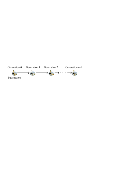
(a) Extreme case 1.

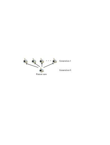
(b) Extreme case 2.

Figure 2: Two extreme cases of worm trees.

Based on these considerations and assumptions, the sequential growth model of a worm tree works as follows: We consider a fixed sequence of infected hosts (i.e., nodes) $v_{1},v_{2},\cdots$ and inductively construct a random worm tree $(T_{n})_{n\geq 1}$, where $n$ is the number of nodes and $T_{1}$ has only patient zero. Infecting a new host is equivalent to adding a new node into the existing worm tree. Hence, given $T_{n-1}$, $T_{n}$ is formed by adding node $v_{n}$ together with an edge directed from an existing node $v_{f}$ to $v_{n}$. According to the assumption, $v_{f}$ is randomly chosen among the $n-1$ nodes in the tree, i.e., $\mbox{Pr}(f=k)=\frac{1}{n-1}$, $k=1,2,\cdots,n-1$. Note that such a growth model and its variations have been widely used in studying topology generators [22, 23]. In this paper, we apply this model to characterize worm infection.

3 Mathematical Analysis

In this section, we study the worm tree through mathematical analysis. Specifically, we first derive the joint distribution of the number of children and the generation, i.e., $p_{n}(i,j)$, by applying probabilistic methods. We then use $p_{n}(i,j)$ to analyze two marginal distributions, i.e., $c_{n}(i)$ and $g_{n}(j)$, and obtain their closed-form approximations. Finally, we find a closed-form approximation to $p_{n}(i,j)$.

3.1 Joint Distribution

For a worm tree with only patient zero (i.e., $n=1$), since $L_{1}(0,0)=1$ with probability 1, $p_{1}(0,0)=1$. Similarly, for a worm tree with $n=2$, it is evident that $L_{2}(1,0)=L_{2}(0,1)=1$. Thus, $p_{2}(1,0)=p_{2}(0,1)=\frac{1}{2}$. We now consider $p_{n}(i,j)$ ($0\leq i,j\leq n-1$) when $n\geq 3$. Specifically, we study two cases:

(1) $p_{n}(0,j)$, i.e., the proportion of the number of leaves in generation $j$ in $T_{n}$. Assume that $T_{n-1}$ is given, and there are $L_{n-1}(0,j)$ leaves in generation $j$ and totally $G_{n-1}(j-1)=\sum_{i=0}^{n-2}{L_{n-1}(i,j-1)}$ nodes in generation $j-1$. Note that we have extended the notation so that $G_{n-1}(-1)=L_{n-1}(i,-1)=0$, $0\leq i\leq n-2$. When a new node $v_{n}$ is added, $v_{n}$ becomes a leaf of $T_{n}$. If $v_{n}$ is connected to one of existing nodes in generation $j-1$, $v_{n}$ belongs to generation $j$; and the probability of such an event is $\frac{G_{n-1}(j-1)}{n-1}$. Moreover, if a leaf in generation $j$ in $T_{n-1}$ connects to $v_{n}$, this node is no longer a leaf and now has one child; and the probability of this event is $\frac{L_{n-1}(0,j)}{n-1}$. Therefore, we can obtain the stochastic recurrence of $L_{n}(0,j)$:

$$L_{n}(0,j)=\left\{\begin{array}[]{l l l}L_{n-1}(0,j)+1,&\mbox{w.p.}\ \ \frac{G_{n-1}(j-1)}{n-1}\\ L_{n-1}(0,j)-1,&\mbox{w.p.}\ \ \frac{L_{n-1}(0,j)}{n-1}\\ L_{n-1}(0,j),&\ \ \mbox{otherwise}.\end{array}\right.$$ (1)

Given $T_{n-1}$ (i.e., $L_{n-1}(0,j)$ and $G_{n-1}(j-1)$), the conditional expected value of $L_{n}(0,j)$ is $\left[L_{n-1}(0,j)+1\right]\cdot\frac{G_{n-1}(j-1)}{n-1}+\left[L_{n-1}(0,j)-1\right]\cdot\frac{L_{n-1}(0,j)}{n-1}+L_{n-1}(0,j)\cdot\left[1-\frac{G_{n-1}(j-1)+L_{n-1}(0,j)}{n-1}\right]$, i.e.,

$$\textstyle\mbox{E}[L_{n}(0,j)|T_{n-1}]=\frac{n-2}{n-1}L_{n-1}(0,j)+\frac{1}{n-1}G_{n-1}(j-1).$$ (2)

Applying $\mbox{E}[L_{n}(0,j)]=\mbox{E}[\mbox{E}[L_{n}(0,j)|T_{n-1}]]$ (i.e., the law of total expectation), we obtain

$$\textstyle\mbox{E}[L_{n}(0,j)]=\frac{n-2}{n-1}\mbox{E}[L_{n-1}(0,j)]+\frac{1}{n-1}\mbox{E}[G_{n-1}(j-1)].$$ (3)

Using the definitions $p_{n}(0,j)=\frac{\mbox{E}[L_{n}(0,j)]}{n}$ and $g_{n-1}(j-1)=\frac{\mbox{E}[G_{n-1}(j-1)]}{n-1}=\sum_{i=0}^{n-2}{p_{n-1}(i,j-1)}$, the above equation leads to

$$p_{n}(0,j) = \textstyle\frac{n-2}{n}p_{n-1}(0,j)+\frac{1}{n}g_{n-1}(j-1)$$ (4)

$$= \textstyle\frac{n-2}{n}p_{n-1}(0,j)+\frac{1}{n}\sum_{i=0}^{n-2}{p_{n-1}(i,j-1)}.$$ (5)

(2) $p_{n}(i,j)$, $1\leq i\leq n-1$. Given $L_{n-1}(i,j)$ and $L_{n-1}(i-1,j)$ in $T_{n-1}$, we study $L_{n}(i,j)$ in $T_{n}$. When the new node $v_{n}$ is added into $T_{n-1}$, $v_{n}$ is connected to a node with $i-1$ children and in generation $j$ with probability $\frac{L_{n-1}(i-1,j)}{n-1}$, or is connected to a node with $i$ children and in generation $j$ with probability $\frac{L_{n-1}(i,j)}{n-1}$. Thus, in $T_{n}$,

$$L_{n}(i,j)=\left\{\begin{array}[]{l l l}L_{n-1}(i,j)+1,&\mbox{w.p.}\ \ \frac{L_{n-1}(i-1,j)}{n-1}\\ L_{n-1}(i,j)-1,&\mbox{w.p.}\ \ \frac{L_{n-1}(i,j)}{n-1}\\ L_{n-1}(i,j),&\ \ \mbox{otherwise}.\end{array}\right.$$ (6)

This relationship leads to

$$\textstyle\mbox{E}[L_{n}(i,j)|T_{n-1}]=\frac{n-2}{n-1}L_{n-1}(i,j)+\frac{1}{n-1}L_{n-1}(i-1,j).$$ (7)

Therefore,

$$\textstyle\mbox{E}[L_{n}(i,j)]=\frac{n-2}{n-1}\mbox{E}[L_{n-1}(i,j)]+\frac{1}{n-1}\mbox{E}[L_{n-1}(i-1,j)].$$ (8)

That is,

$$\textstyle p_{n}(i,j)=\frac{n-2}{n}p_{n-1}(i,j)+\frac{1}{n}{p_{n-1}(i-1,j)}.$$ (9)

Summarizing the above two cases, we have the following theorem:

Theorem 1

When $n\geq 3$, the joint distribution of the number of children and the generation in a worm tree $T_{n}$ follows

$$p_{n}(i,j)=\left\{\begin{array}[]{l l l}\frac{n-2}{n}p_{n-1}(0,j)+\frac{1}{n}g_{n-1}(j-1),&i=0\\ \frac{n-2}{n}p_{n-1}(i,j)+\frac{1}{n}{p_{n-1}(i-1,j)},&\mbox{otherwise},\end{array}\right.$$ (10)

where $0\leq i,j\leq n-1$.

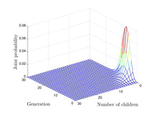
Figure 3: Joint distribution of the number of children and the generation ($n=2000$).

Theorem 10 provides a way to calculate $p_{n}(i,j)$ recursively from $p_{2}(i,j)$. Fig. 3 shows a snapshot of $p_{n}(i,j)$ when $n=2000$. It can be seen that when the generation is specified (i.e., $j$ is fixed), $p_{n}(i,j)$ is a monotonous function and decreases quickly as $i$ increases. On the other hand, when the number of children is given (i.e., $i$ is fixed), $p_{n}(i,j)$ has a bell shape. Moreover, since $\sum_{i=0}^{10}{\sum_{j=0}^{15}{p_{n}(i,j)}}=0.9976$, most nodes do not have a large number of children, and the worm tree does not have a large average path length.

3.2 Number of Children

We use $p_{n}(i,j)$ to derive the marginal distribution of the number of children, i.e., $c_{n}(i)$. Similarly, we study two cases:

(1) $c_{n}(0)$, i.e., the proportion of the number of leaves in $T_{n}$. Since $c_{n}(0)=\sum_{j=0}^{n-1}{p_{n}(0,j)}$ and $\sum_{j=0}^{n-1}g_{n-1}(j-1)=1$, we obtain the recursive relationship of $c_{n}(0)$ from Equation (4):

$$\textstyle c_{n}(0)=\frac{n-2}{n}c_{n-1}(0)+\frac{1}{n}.$$ (11)

Moreover, note that $c_{2}(0)=\frac{1}{2}$. If we assume that $c_{n-1}(0)=\frac{1}{2}$, we can obtain by induction that

$$c_{n}(0)=\textstyle\frac{1}{2}.$$ (12)

This indicates that no matter how many nodes are in the worm tree, on average half of nodes are leaves, i.e., on average 50% of infected hosts never compromise any target.

(2) $c_{n}(i)$, $1\leq i\leq n-1$. From Equation (9) and $c_{n}(i)=\sum_{j=0}^{n-1}{p_{n}(i,j)}$, we find the recurrence of $c_{n}(i)$ as follows

$$\textstyle c_{n}(i)=\frac{n-2}{n}c_{n-1}(i)+\frac{1}{n}c_{n-1}(i-1).$$ (13)

Summarizing the above two cases, we have the following theorem on the distribution of the number of children:

Theorem 2

When $n\geq 3$, the distribution of the number of children in a worm tree $T_{n}$ follows

$$c_{n}(i)=\left\{\begin{array}[]{l l l}\frac{1}{2},&i=0\\ \frac{n-2}{n}c_{n-1}(i)+\frac{1}{n}c_{n-1}(i-1),&1\leq i\leq n-1.\end{array}\right.$$ (14)

From Theorem 14, we can derive the statistical properties of the number of children as follows.

Corollary 1

When $n\geq 1$, the expectation and the variance of the number of children are

$$\textstyle\mbox{E}_{n}[C]=\sum_{i=0}^{n-1}{i\cdot c_{n}(i)}=\frac{n-1}{n}$$ (15)

$$\textstyle\mbox{Var}_{n}[C]=\sum_{i=0}^{n-1}{\left(i-\mbox{E}_{n}[C]\right)^{2}\cdot c_{n}(i)}=2-\frac{n-1}{n^{2}}-\frac{2H_{n}}{n},$$ (16)

where $H_{n}=\sum\nolimits_{i=1}^{n}{\frac{1}{i}}$ is the $n$-th harmonic number [20].

The proof of Corollary 1 is given in Appendix 1. One intuitive way to derive $\mbox{E}_{n}[C]$ is that in worm tree $T_{n}$, there are $n-1$ directed edges and $n$ nodes. Thus, the average number of edges (i.e, the average number of children) of a node is $\frac{n-1}{n}$. Moreover, since $H_{n}$ is $O(1+\ln{n})$, $\mathop{\lim}\limits_{n\to\infty}\mbox{E}_{n}[C]=1$, and $\mathop{\lim}\limits_{n\to\infty}\mbox{Var}_{n}[C]=2$.

Theorem 14 also leads to a simple closed-form expression of the distribution of the number of children when $n$ is very large, as shown in the following corollary.

Corollary 2

When $n\rightarrow\infty$, the number of children has a geometric distribution with parameter $\frac{1}{2}$, i.e.,

$$c(i)=\mathop{\lim}\limits_{n\to\infty}c_{n}(i)=\Big{(}\frac{1}{2}\Big{)}^{i+1},\ \ i=0,1,2,\cdots.$$ (17)

The proof of Corollary 17 is given in Appendix 2. Corollary 17 indicates that when $n$ is very large, $c_{n}(i)$ decreases approximately exponentially with a decay constant of $\ln 2$ as the number of children increases.

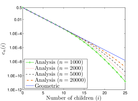
Figure 4: Distribution of the number of children.

We further study when both $n$ and $i$ are finite and large, how $c_{n}(i)$ varies with $n$, i.e., how the tail of the distribution of the number of children changes with $n$. First, note that $c_{3}(0)=\frac{1}{2}$, $c_{3}(1)=\frac{1}{3}$, and $c_{3}(2)=\frac{1}{6}$. Thus, from Equation (13), we can prove by induction that $c_{n}(i)$ ($n\geq 3$) is a decreasing function of $i$, i.e., $c_{n}(i)<c_{n}(i-1)$, for $1\leq i\leq n-1$. Next, putting this inequality into Equation (13), we have $c_{n}(i)>\frac{n-1}{n}c_{n-1}(i)$. Hence, when $n$ is very large, $\frac{n-1}{n}\approx 1$, and $c_{n}(i)>c_{n-1}(i)$, which indicates that the tail of $c_{n}(i)$ increases with $n$. Fig. 4 verifies this result, showing $c_{n}(i)$ obtained from Theorem 14 when $n=1000$, $2000$, $5000$, and $20000$, as well as the geometric distribution with parameter 0.5 obtained from Corollary 17. Note that the y-axis uses log-scale. It can be seen that when $n$ increases from 1000 to 20000, the tail of $c_{n}(i)$ also increases to approach the tail of the geometric distribution. Moreover, it is shown that the geometric distribution well approximates the distribution of the number of children when $n$ is large.

3.3 Generation

Next, we derive the generation distribution (i.e., $g_{n}(j)$) in a similar manner to the case of $c_{n}(i)$. Using Theorem 10 and $g_{n}(j)=\sum_{i=0}^{n-1}{p_{n}(i,j)}$, we obtain the following theorem:

Theorem 3

When $n\geq 3$, the distribution of the generation in a worm tree $T_{n}$ follows

$$\textstyle g_{n}(j)=\frac{n-1}{n}g_{n-1}(j)+\frac{1}{n}g_{n-1}(j-1),0\leq j\leq n-1,$$ (18)

where $g_{n-1}(-1)=0$.

Theorem 3 gives a method to calculate the distribution of the generation recursively. Moreover, from Theorem 3, we can derive the statistical properties of the generation distribution in the following corollary.

Corollary 3

When $n\geq 1$, the expectation and the variance of the generation are

$$\textstyle\mbox{E}_{n}[G]=\sum_{j=0}^{n-1}{j\cdot g_{n}(j)}=H_{n}-1.$$ (19)

$$\textstyle\mbox{Var}_{n}[G]=\sum_{j=0}^{n-1}{\left(j-\mbox{E}_{n}[G]\right)^{2}\cdot g_{n}(j)}=H_{n}-H_{n,2},$$ (20)

where $H_{n}=\sum\nolimits_{i=1}^{n}{\frac{1}{i}}$ and $H_{n,2}=\sum\nolimits_{i=1}^{n}{\frac{1}{i^{2}}}$.

The proof of Corollary 3 is given in Appendix 3. From Corollary 3, we have some interesting observations. Since $H_{n}$ is $O(1+\ln{n})$ and $H_{\infty,2}=\zeta(2)=\frac{\pi^{2}}{6}\approx 1.645$ is the Riemann zeta function of 2 [24], both $\mbox{E}_{n}[G]$ and $\mbox{Var}_{n}[G]$ are $O(1+\ln{n})$. This indicates that the average path length of the worm tree (i.e., $\mbox{E}_{n}[G]$) increases approximately logarithmically with $n$. Moreover, when $n\rightarrow\infty$, $\mathop{\lim}\limits_{n\to\infty}\mbox{E}_{n}[G]-\ln{n}=\gamma-1$, and $\mathop{\lim}\limits_{n\to\infty}\mbox{Var}_{n}[G]-\ln{n}=\gamma-\zeta(2)$, where $\gamma\approx 0.577$ is the Euler-Mascheroni constant [25]. Therefore, when $n$ is large, $\mbox{E}_{n}[G]\approx\mbox{Var}_{n}[G]$. Furthermore, we can use Theorem 3 to obtain a closed-form approximation to $g_{n}(j)$ as follows.

Corollary 4

When $n$ is very large, the generation distribution $g_{n}(j)$ can be approximated by a Poisson distribution with parameter $\lambda_{n}=\mbox{E}_{n}[G]=H_{n}-1$. That is,

$$\textstyle g_{n}(j)\approx\frac{\lambda_{n}^{j}}{j!}e^{-\lambda_{n}},\ \ 0\leq j\leq n-1.$$ (21)

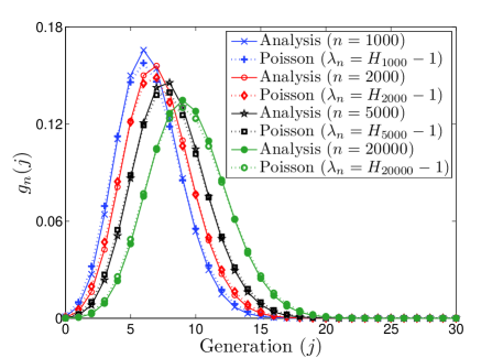
Figure 5: Distribution of the generation.

The proof of Corollary 4 is given in Appendix 4. Fig. 5 verifies Corollary 4, showing $g_{n}(j)$ obtained from Theorem 3 when $n=1000$, $2000$, $5000$, and $20000$, as well as the Poisson distribution with parameter $\mbox{E}_{n}[G]$. It can be seen that when $n$ is large, the Poisson distribution fits the generation distribution closely.

3.4 Approximation to the Joint Distribution

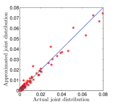
Figure 6: Parity plot of the approximation to the joint distribution ($n=2000$).

Finally, we derive a closed-form approximation to the joint distribution $p_{n}(i,j)$. From Equation (9), we can see that when $n\to\infty$, $p_{n}(i,j)=p_{n-1}(i,j)$, which yields

$$\textstyle p_{n}(i,j)=\frac{1}{2}p_{n}(i-1,j).$$ (22)

Hence, we can obtain

$$\textstyle p_{n}(i,j)=\left(\frac{1}{2}\right)^{i}p_{n}(0,j)\approx\left(\frac{1}{2}\right)^{i+1}g_{n}(j).$$ (23)

Since when $n$ is very large, $g_{n}(j)$ follows closely the Poisson distribution as in Corollary 4,

$$\textstyle p_{n}(i,j)\approx\left(\frac{1}{2}\right)^{i+1}\cdot\frac{\lambda_{n}^{j}}{j!}e^{-\lambda_{n}},\ \ 0\leq i,j\leq n-1,$$ (24)

where $\lambda_{n}=H_{n}-1$. The above derivation also shows that when $n$ is very large, the number of children and the generation are almost independent random variables.

Fig. 6 shows the parity plot of the approximation to the joint distribution when $n=2000$. In the figure, the x-axis is the actual $p_{n}(i,j)$ obtained from Theorem 10, and the y-axis is the approximated $p_{n}(i,j)$ from Equation (24), where $0\leq i,j\leq 30$. It can be seen that most points are on or near the diagonal line, indicating that the approximation to the joint distribution is reasonable.

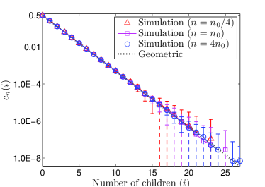
(a) Number of children.

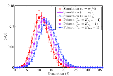
(b) Generation.

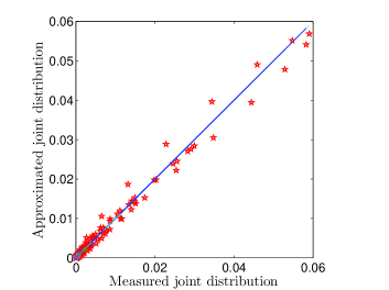
(c) Joint distribution ($n=n_{0}$).

Figure 7: Simulating the infection structure of the Code Red v2 worm ($n_{0}=360000$).

4 Simulations and Verification

In this section, we study the worm infection structure through simulations. As far as we know, there is no publicly available data to show the real worm tree and verify our analytical results. Moreover, real experiments in a controlled environment are impractical for this study since the closed-form approximations are derived based on the assumption that the number of nodes is very large. Therefore, we apply empirical simulations. Specifically, we first simulate the infection structure of the Code Red v2 worm and then study the effects of important parameters on the worm tree. Finally, we extend our simulation to localized-scanning worms.

4.1 Code Red v2 Worm Verification

We simulate the propagation of the Code Red v2 worm by using and extending the simulator in [26]. Specifically, the simulator considers a discrete-time system and mimics the random-scanning behavior of infected hosts during each discrete time interval. Moreover, the parameter setting is based on the Code Red v2 worm’s characteristics. For example, the vulnerable population is $n_{0}=360,000$, and a newly infected host is assigned with a scanning rate of 358 scans/min. Detailed information about how the parameters are chosen can be found in Section VII of [27]. We then extend the simulator to track the worm infection structure by adding the information of the number of children and the generation to each infected host. Moreover, we set the time unit to 20 seconds and start our simulation at time tick 0 with patient zero. Note that we remove the assumption used in the sequential growth model that no two hosts are compromised at the same time. That is, multiple hosts can be compromised at one time tick. Moreover, all new victims of the current time tick start scanning at the next time tick. The simulation results (mean $\pm$ standard deviation) are obtained from 100 independent runs with different seeds and are presented in Fig. 7.

Fig. 7(a) shows the distribution of the number of children, comparing the simulation results of $c_{n}(i)$ for $n={n_{0}}/{4}$, $n_{0}$, and $4n_{0}$ with the geometric distribution obtained from Corollary 17. Note that the y-axis uses the log-scale. The dotted line represents the standard deviation that goes into the negative territory. It can be seen that the distribution of the number of children can be well approximated by the geometric distribution with parameter 0.5. This implies that $c_{n}(i)$ decreases approximately exponentially with a decay constant of $\ln{2}$. Specifically, in all three cases, on average 50.0% of the infected hosts do not have children, about 98.4% of them have no more than five children, and 0.1% of them have no less than ten children. We also calculate the expectation and the variance of the number of children from the simulation and find that they are identical to the analytical results obtained from Corollary 1. Fig. 7(b) demonstrates the generation distribution, comparing the simulation results of $g_{n}(j)$ for $n={n_{0}}/{4}$, $n_{0}$, and $4n_{0}$ with the Poisson distributions with parameter $\mbox{E}_{n}[G]=H_{n}-1$ obtained from Corollary 4. It can be seen that the simulation results of $g_{n}(j)$ closely follow the Poisson distributions for all three cases. Hence, simulation results verify that the average path length of the worm tree increases approximately logarithmically with the total number of infected hosts. Moreover, we also compute the expectation and the variance of the generation in simulations and verify the analytical results in Corollary 3. Fig. 7(c) compares the measured joint distribution from simulations with the approximated joint distribution from Equation (24) by using the parity plot. It can be seen that most points are on or near the diagonal line, indicating that the approximation works well.

4.2 Effects of Worm Parameters

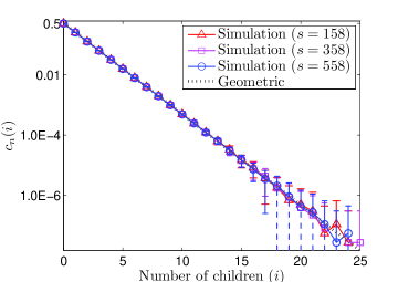
(a) Effect of scanning rates on $c_{n}(i)$.

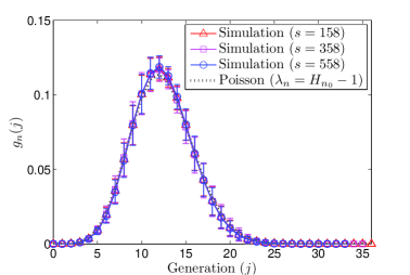
(b) Effect of scanning rates on $g_{n}(j)$.

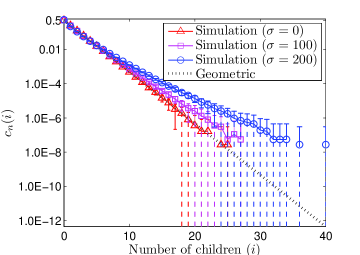
(c) Effect of scanning rate standard deviation on $c_{n}(i)$.

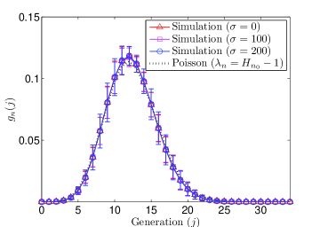
(d) Effect of scanning rate standard deviation on $g_{n}(j)$.

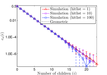
(e) Effect of hitlist sizes on $c_{n}(i)$.

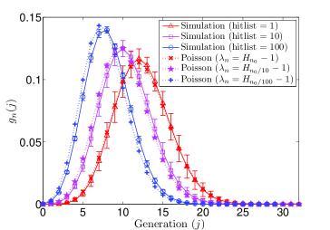
(f) Effect of hitlist sizes on $g_{n}(j)$.

Figure 8: Effects of the scanning rate, the scanning rate standard deviation, and the hitlist size on the distributions of the number of children and the generation ($n_{0}=360000$).

Next, we extend our simulator to examine the effects of three important parameters of worm propagation on the worm tree: the scanning rate, the scanning rate standard deviation, and the hitlist size. When a parameter is studied and varied, we set other parameters to the parameters of the Code Red v2 worm as used in Section 4.1. The simulation results are obtained from 100 independent simulation runs and are shown in Fig. 8.

Fig.s 8(a) and (b) show the effect of varying the scanning rate $s$ (scans/min) from 158 to 558 on the distributions of the number of children and the generation. Here, the scanning rate is set to a fixed value for every infected host, i.e., the scanning rate standard deviation is 0. The figures also plot the geometric distribution with parameter 0.5 and the Poisson distribution with parameter $H_{n_{0}}-1$ for reference. It can be seen that the scanning rate does not affect the worm tree structure.

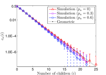
(a) Number of children.

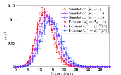
(b) Generation.

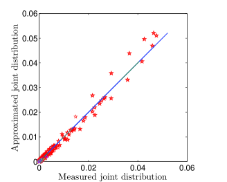
(c) Joint distribution ($p_{a}=0.6$).

Figure 9: Simulating the infection structure of the localized-scanning worm ($n=360000$, $s=358$ scans/min, $\sigma=0$, $hitlist=1$, and $l=8$).

Fig.s 8(c) and (d) demonstrate the effect of the variation of the scanning rates among different hosts (i.e., $\sigma$). In our simulation, a newly infected host is assigned with a scanning rate (scans/min) from a normal distribution $N(358,\sigma^{2})$. The figures show the simulation results when $\sigma=0$, $100$, and $200$. It can be seen that while the scanning rate standard derivation $\sigma$ has no effect on the generation distribution, it does affect the distribution of the number of children. Specifically, when $\sigma$ increases, the tail of $c_{n}(i)$ moves upward from the geometric distribution with parameter 0.5. This is because when $\sigma$ becomes larger, the variation of the scanning rate among infected hosts is greater. That is, there are more hosts with high scanning rates and also more hosts with low scanning rates. As a result, those hosts with high scanning rates tend to infect a large number of hosts, making the tail of $c_{n}(i)$ move upward. However, it is also observed that when $\sigma$ is not very large (the case for real worms), the geometric distribution with parameter 0.5 is still a good approximation.

In Fig.s 8(e) and (f), we show the effect of the hitlist size on the worm tree. As pointed out in Section 2, when the hitlist size is greater than 1, the underlying infection topology is a worm forest with the number of trees equal to the hitlist size. Moreover, in a worm forest, it is intuitive that each tree is a smaller version of the single worm tree of hitlist size 1 and has fewer nodes. Hence, it is not surprising to see that in Fig. 8(f), the generation distribution moves leftward when the hitlist size increases. However, the generation distribution can still be well approximated by the Poisson distribution with parameter $H_{n_{h}}-1$, where $n_{h}$ is the average number of nodes in a tree. Moreover, since in each tree the distribution of the number of children can be approximated by the geometric distribution with parameter 0.5, in the worm forest $c_{n}(i)$ still follows closely the same distribution.

4.3 Localized Scanning

Finally, we extend our simulation study to the infection tree of localized-scanning worms. Different from random scanning, localized scanning preferentially searches for targets in the “local” address space [8]. As a result, when a new node is added to the worm tree, it connects to one of the existing nodes that are in the same “local” address space with a higher probability. That is, the growth model is no longer uniform attachment as studied in Section 3. For simplicity, in this paper we only consider the $/l$ localized scanning [19]:

• Local scanning: $p_{a}(0\leq p_{a}<1)$ of the time, a “local” address with the same first $l$ ($0\leq l\leq 32$) bits as the attacking host is chosen as the target.

• Global scanning: $1-p_{a}$ of the time, a random address is chosen.

Note that random scanning can be regarded as a special case of localized scanning when $p_{a}=0$. Moreover, if local scanning is selected, it can be regarded as random scanning in a local $/l$ subnet. It has been shown that since the vulnerable-hosts distribution is highly uneven, localized scanning can spread a worm much faster than random scanning [18, 21].

We extend our simulator to imitate the spread of localized-scanning worms. We extract the distribution of vulnerable hosts in $/l$ subnets from the dataset provided by DShield [28, 29]. Specifically, we use the dataset in [29] with port 80 (HTTP) that is exploited by the Code Red worm to generate the vulnerable-host distribution. Moreover, we use similar parameters as in Section 4.1 (e.g., $n=360000$, $s=358$ scans/min, $\sigma=0$, and $hitlist=1$) and set the subnet level to 8 (i.e., $l=8$). The results are obtained from 100 independent simulation runs and are shown in Fig. 9. For each run, patient zero is randomly chosen from vulnerable hosts.

Fig. 9(a) compares the simulation results of the distributions of the number of children (i.e., $c_{n}(i)$) when $p_{a}=0$, 0.3, and 0.6 with the geometric distribution with parameter 0.5. It is surprising that $c_{n}(i)$ of localized-scanning worms can still be well approximated by the geometric distribution. That is, the majority of nodes have few children, whereas a small portion of compromised hosts infect a large number of hosts. An intuitive explanation is given as follows. From Fig. 7(a), it can be seen that the total number of nodes has a minor effect on $c_{n}(i)$. Hence, if in a /8 subnet the majority of vulnerable hosts are infected through local scanning, it is expected that $c_{n}(i)$ of these hosts still closely follows the geometric distribution since the local scanning can be regarded as random scanning inside a /8 subnet. Therefore, both local infection and global infection lead $c_{n}(i)$ towards the geometric distribution with parameter 0.5. On the other hand, it can also be seen that when $p_{a}$ increases, the tail of $c_{n}(i)$ moves slightly downward. This is because as $p_{a}$ increases, more vulnerable hosts are infected through local scanning. Hence, it is more difficult for an infected host to find targets after vulnerable hosts in this host’s local subnet have been exhausted. As a result, when $p_{a}$ increases, fewer nodes can have a large number of children.

Fig. 9(b) demonstrates that the generation distribution of localized-scanning worms (i.e., $g_{n}(j)$) can be well approximated by the Poisson distribution for the cases of $p_{a}=0$, 0.3, and 0.6. The Poisson parameter, however, depends not only on $n$, but also on $p_{a}$. We further define $\lambda_{n}^{p_{a}}=\mbox{E}_{n}^{p_{a}}[G]$ as the expectation of the generation for a localized-scanning worm with parameter $p_{a}$. Here, $\mbox{E}_{n}^{p_{a}}[G]$ can be easily estimated from the simulation results of $g_{n}(j)$. Fig. 9(c) further shows the parity plot of the simulated joint distribution and the approximated joint distribution from Equation (24) when $p_{a}=0.6$. Since most points are on or near the diagonal line, the approximation is reasonable.

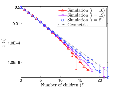
Figure 10: Effect of the subnet level ($p_{a}=0.6$).

Moreover, Fig. 10 shows the effect of the subnet level (i.e., $l$) on the distribution of the number of children (i.e., $c_{n}(i)$). It can be seen that when $l$ increases, the tail of $c_{n}(i)$ moves downward. The reason is similar to the argument used in Fig. 9(a), i.e., as $l$ increases, fewer nodes can infect a large number of children. However, the figure also demonstrates that the geometric distribution with parameter 0.5 is still a good approximation to $c_{n}(i)$, especially when the number of children is not large.

5 Applications of Observations

Our observations on the topologies formed by worm infection have important implications and applications for both defenders and attackers. For example, we have found that the generation distribution closely follows the Poisson distribution and the average path length increases approximately logarithmically with the number of nodes. On one hand, some schemes have been proposed to trace worms back to their origins through the cooperation between infected hosts [30, 31], and our work quantifies the average path length that describes a lower bound of the number of hosts required to cooperate. On the other hand, this average path length reflects the delay or the effort for a botmaster to deliver a command to all bots in a P2P-based botnet like Conficker C, and our results show that the botnet is scalable and can efficiently forward commands to a large number of bots. In this section, we focus on the applications of the distribution of the number of children for both defenders and attackers. Specifically, we study a simple and efficient bot detection method in a Conficker C like P2P-based botnet and consider a countermeasure by future botnets.

5.1 Bot Detection

We consider a P2P-based botnet formed by worm scanning/infection. That is, once a host infects another host, they become peers in the resulting P2P-based botnet. When a defender captures an infected host in a botnet, the defender can process the historic records inside the host or monitor the traffic going into or out of the host, and will potentially detect other infected hosts such as the father and the children of this infected host. Then, our question is that if a defender can only access a small portion of nodes in a botnet, how many bots will be detected by the defender. Moreover, inspired by the random removal and targeted removal methods used in analyzing the robustness of a topology [13], here we study two bot detection strategies:

• Random detection: Access bots randomly.

• Targeted detection: Access bots that have the largest number of children.

Analytically, we suppose that a defender can access a small ratio of bots in a botnet. We assume that an accessed bot exposes itself, its father, and its children to the defender. To simplify the analysis, we also assume that the accessed bot ratio, $A$, is a power of 0.5 and all exposed nodes are different nodes. We then calculate the average percentages of exposed bots by random detection and targeted detection.

Since from Corollary 1 a randomly selected node has approximately one child, the average percentage of bots that can be exposed by random detection is then

$$\textstyle D_{R}=3A.$$ (25)

For targeted detection, since the nodes with the largest number of children are chosen and the number of children follows asymptotically a geometric distribution with parameter 0.5 as shown in Corollary 17,

$$\textstyle A=\sum_{i\geq d}{c_{n}(i)}=\sum_{i=d}^{\infty}{\left(\frac{1}{2}\right)^{i+1}}=\left(\frac{1}{2}\right)^{d},$$ (26)

where $d$ is the smallest number of children of accessed nodes. That is, $d=-\log_{2}{A}$. Therefore, the average percentage of exposed nodes by targeted detection is

$$\textstyle D_{T}=\sum_{i=d}^{\infty}{(2+i)\cdot c_{n}(i)}=(d+3)\left(\frac{1}{2}\right)^{d}=A(3-\log_{2}A).$$ (27)

Compared with random detection, targeted detection can expose $(-A\log_{2}A)\times n$ more nodes. For example, if $A=\frac{1}{64}$, on average random detection can detect 4.69% of nodes, whereas targeted detection can expose 14.06% of bots.

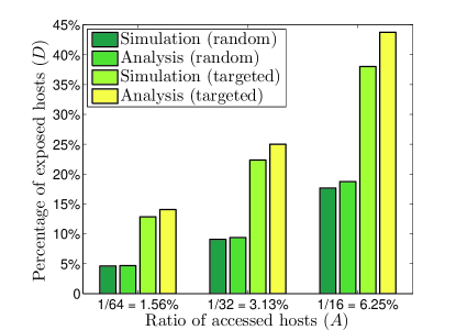
Figure 11: Random and targeted detection.

We then extend our simulation in Section 4.1 to study the effectiveness of random and targeted detection strategies. Fig. 11 shows the simulation results over 100 independent runs for both strategies, as well as the analytical results from Equations (25) and (27), when $A=\frac{1}{64}$, $\frac{1}{32}$, and $\frac{1}{16}$. It can be seen that the analytical results slightly overestimate the exposed host percentage. This is because in our analysis we ignore the case that two exposed nodes can be duplicate. Fig. 11 also demonstrates that targeted detection performs much better than random detection. For example, in our simulation, when $A=3.125\%$, 9.10% of the bots are exposed under random detection, whereas 22.36% of the bots are detected under targeted detection. Therefore, when a small portion of bots are examined, the botnets formed by worm infection are robust to random detection, but are relatively vulnerable to targeted detection.

5.2 A Countermeasure by Future Botnets

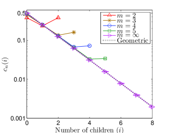
(a) Distribution of the number of children.

(b) Targeted detection.

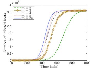
(c) Worm propagation speed.

Figure 12: A worm countermeasure via limiting the maximum number of children.

To counteract the targeted detection method, an intuitive way for botnets is to limit the maximum number of children for each node. That is, set a small number $m$. Once an infected host has compromised $m$ other hosts, this host stops scanning. In this way, there is no node with a large number of children. Moreover, the infected hosts can self-stop scanning, potentially reducing the worm traffic [32].

To analyze the robustness of such botnets against targeted detection, we extend Corollary 17 to obtain an approximated distribution of the number of children in a botnet with the countermeasure:

$$c_{n}(i)=\left\{\begin{array}[]{l l l}\left(\frac{1}{2}\right)^{i+1},&i=0,1,2,\cdots,m-1\\ \left(\frac{1}{2}\right)^{m},&i=m.\end{array}\right.$$ (28)

The distribution is based on the observation that those nodes having more than $m$ children in a botnet without the countermeasure can now have only $m$ children. Hence, the expected percentage of exposed nodes under targeted detection can be calculated:

$$D_{T}^{\prime}=\left\{\begin{array}[]{l l l}(m+2)\cdot A,&A\leq\left(\frac{1}{2}\right)^{m}\\ A(3-\log_{2}A)-\left(\frac{1}{2}\right)^{m},&A>\left(\frac{1}{2}\right)^{m}.\end{array}\right.$$ (29)

Compared with $D_{T}$ in Equation (27), $D_{T}^{\prime}$ is smaller. This means that under the countermeasure the number of exposed nodes can be reduced significantly. For example, when $m=3$ and $A=\frac{1}{64}$, $D_{T}=\frac{9}{64}$, and $D_{T}^{\prime}=\frac{5}{64}$.

We then extend our simulation in Section 5.1 to simulate the worm tree generated using the above countermeasure and evaluate its performance against targeted detection. Fig. 12(a) shows the distribution of the number of children when $m=2$, 3, 4, and 5. It can be seen that except for $m=2$, $c_{n}(i)$ is well approximated by Equation (28). For $m=2$, since an infected host stops scanning when it has hit two vulnerable hosts, leaves in the worm tree have more chances to recruit a child. Fig. 12(b) demonstrates the expected percentage of exposed nodes (i.e., $D_{T}^{\prime}$), when $A=\frac{1}{64}$, $\frac{1}{32}$, and $\frac{1}{16}$, and $m=2$, 3, 4, and 5. It can be seen that $D_{T}^{\prime}$ follows approximately the analytical results in Equation (29). Moreover, the expected percentage of exposed nodes under the countermeasure is reduced significantly. For example, when $A=\frac{1}{32}$, the percentage is reduced from 22.36% without the countermeasure to 19.80%, 15.99%, 12.58%, and 9.38% when $m=5$, 4, 3, and 2, respectively.

On the other hand, since not every infected host keeps scanning the targets, the countermeasure can potentially slow down the speed of worm infection. Thus, we also simulate the propagation speed of worms that limit the maximum number of children and plot the results in Fig. 12(c) for $m=2$, 3, 4, and 5, as well as the original worm without the countermeasure. It can be seen that except for $m=2$, the worm does not slow down much. But even when $m=2$, the worm can infect most vulnerable hosts within 17 hours. Moreover, Fig.s 12(b) and (c) demonstrate the tradeoff between the efficiency of worm infection and the robustness of the formed botnet topology. That is, a worm with the countermeasure spreads slower, but the resulting botnet is more robust against targeted detection.

6 Related work

Since the Code Red worm in 2001, Internet worms have been an active research topic. Many mathematical models have been developed to characterize the spread of worms, estimate worm behaviors, and contain worm propagation. Most models, however, have focused on the macro-level behavior of worm infection. Specifically, different analytical approaches have been applied to study the total number of infected hosts over time [8, 9, 10, 11, 12, 2, 27]. For example, Staniford et al. used a simple differential equation to estimate the global propagation speed of the Code Red v2 worm [8], whereas Rohloff et al. applied a stochastic model to reflect the variation of the number of infected hosts at the early stage of worm infection [11]. The models of the micro-level of worm infection, however, have been investigated little. In this paper, we apply probabilistic modeling methods and reveal some key micro-level information, such as the infection ability of individual hosts and the underlying botnet topology formed by worm infection.

Some efforts have been focused on studying the “who infects whom” information or the worm infection sequence [30, 33, 31, 34]. Different from our work, the prior work investigates the details of the random number generator of worm propagation [30] or infers the worm infection sequence through the observations of network telescopes [33, 34]. Moreover, Sellke et al. applied a branching process to study the effectiveness of a containment strategy [35]. They assume that the total number of scans of an infected host is bounded. As a result, the worm tree studied in their work is fundamentally different from the one in our work.

Botnets have become the top threat to the Internet in recent years. It has been shown that in current botnets, worm infection is still a main tool for recruiting new bots or collecting network information, and random scanning has been widely used [3]. Moreover, botnets are rapidly transiting from IRC systems to P2P systems. In [36], Wang et al. gave a systematic study on P2P-based botnets; whereas in [14], Dagon et al. surveyed different P2P-based botnet topologies, such as random graphs and power-law topologies. Several methods have been proposed to construct P2P-based botnets through worm infection and re-infection [4, 5].

Modeling the topology generation process has been an active research area. For example, Barabási et al. developed the well-known Barabási-Albert (BA) model and used a mean-field approach to characterize the growth of a topology with both preferential attachment and uniform attachment [22, 23]. Moreover, two exact mathematical models have been studied for the BA model [37, 38]. From the theoretical aspect, our proposed worm tree is similar to the random tree. For example, Devroye used the records theory to derive the distribution of the level of a random ordered tree in [39]. Compared with these theoretical efforts, our work studies a very different problem (i.e., botnets formed by worm infection) and uses a very different approach (i.e., probabilistic modeling).

7 Conclusions

In this paper, we attempt to capture the key characteristics of the Internet worm infection family tree and apply them to bot detection. We have shown analytically and empirically that for the infection tree formed by a wide class of worms, the number of children asymptotically has a geometric distribution with parameter 0.5; and the generation closely follows a Poisson distribution with parameter $\mbox{E}_{n}[G]$ (i.e., $H_{n}-1$). As a result, on average half of infected hosts never compromise any target, over 98% of nodes have no more than five children, and a small portion of hosts have a large number of children. Moreover, the average path length of the worm tree increases approximately logarithmically with the number of nodes. We have also demonstrated empirically that similar observations can be found in localized-scanning worms. We have then applied the observations to bot detection and found that targeted detection is an efficient way to expose bots in a botnet. However, we have also pointed out that a simple countermeasure by future botnets can weaken the performance of targeted detection, without greatly slowing down the speed of worm infection.

As part of our ongoing work, we plan to study in more depth efficient methods against future botnets and relax our assumptions to include more worm dynamics. For example, we are studying the effect of user defenses on the worm tree [40].

APPENDIX 1: Proof of Corollary 1

We apply z-transform to derive the expectation and the variance of the number of children. First, note that Corollary 1 holds for $n=1$ and $2$. Next, when $n\geq 3$, we define z-transform

$$\textstyle X_{n}(z)=\sum_{i=0}^{n-1}{c_{n}(i)z^{-i}}.$$ (30)

Setting $c_{n-1}(-1)=1$, we can transform Theorem 14 to

$$\textstyle c_{n}(i)=\frac{n-2}{n}c_{n-1}(i)+\frac{1}{n}c_{n-1}(i-1),\ 0\leq i\leq n-1,$$ (31)

when $n\geq 3$. Then, putting Equation (31) into Equation (30), we can obtain the difference equation of z-transform

$$\textstyle X_{n}(z)=\left(\frac{1}{n}z^{-1}+\frac{n-2}{n}\right)X_{n-1}(z)+\frac{1}{n}.$$ (32)

Note that $\mbox{E}_{n}[C]=-\frac{dX_{n}(z)}{dz}\mid_{z=1}$ and $X_{n-1}(1)=1$, which leads to

$$\textstyle\mbox{E}_{n}[C]=\frac{n-1}{n}\mbox{E}_{n-1}[C]+\frac{1}{n}.$$ (33)

Since $\mbox{E}_{2}[C]=\frac{1}{2}$, we can show by induction that

$$\textstyle\mbox{E}_{n}[C]=\frac{n-1}{n}.$$ (34)

Moreover, $\mbox{E}_{n}[C^{2}]=\frac{d}{dz}\left[z\frac{dX_{n}(z)}{dz}\right]\mid_{z=1}$ yields

$$\mbox{E}_{n}[C^{2}] = \textstyle\frac{n-1}{n}\mbox{E}_{n-1}[C^{2}]+\frac{2}{n}\mbox{E}_{n-1}[C]+\frac{1}{n}$$ (35)

$$= \textstyle\frac{n-1}{n}\mbox{E}_{n-1}[C^{2}]+\frac{3n-5}{n^{2}}.$$ (36)

Thus, we can use $\mbox{E}_{2}[C^{2}]=\frac{1}{2}$ to prove by induction that

$$\textstyle\mbox{E}_{n}[C^{2}]=2+\frac{(n-1)(n-2)}{n^{2}}-\frac{2H_{n}}{n},$$ (37)

where $H_{n}=\sum_{i=1}^{n}{\frac{1}{i}}$ is the $n$-th harmonic number [20]. Therefore,

$$\mbox{Var}_{n}[C] = \textstyle\mbox{E}_{n}[C^{2}]-\mbox{E}_{n}^{2}[C]$$ (38)

$$= \textstyle 2-\frac{n-1}{n^{2}}-\frac{2H_{n}}{n}.$$ (39)

APPENDIX 2: Proof of Corollary 2

It is already known that $c(0)=\frac{1}{2}$. When $i\geq 1$, this corollary follows readily from Equation (13). Since $n\rightarrow\infty$, $c_{n-1}(i)=c_{n}(i)=c(i)$, which yields

$$c(i)=\textstyle\frac{n-2}{n}c(i)+\frac{1}{n}c(i-1).$$ (40)

That is,

$$c(i)=\textstyle\frac{1}{2}c(i-1),\ \ i\geq 1.$$ (41)

Hence, from $c(0)=\frac{1}{2}$, we can recursively obtain

$$c(i)=\textstyle\big{(}\frac{1}{2}\big{)}^{i+1},\ \ i\geq 0.$$ (42)

APPENDIX 3: Proof of Corollary 3

Similar to the proof of Corollary 1, we apply z-transform to derive the expectation and the variance of the generation. First, note that Corollary 3 holds for $n=1$ and $2$. Next, when $n\geq 3$, we define z-transform

$$\textstyle Y_{n}(z)=\sum_{j=0}^{n-1}{g_{n}(j)z^{-j}}.$$ (43)

Putting Equation (18) into Equation (43), we can obtain the difference equation of z-transform

$$\textstyle Y_{n}(z)=\left(\frac{1}{n}z^{-1}+\frac{n-1}{n}\right)Y_{n-1}(z).$$ (44)

Note that $\mbox{E}_{n}[G]=-\frac{dY_{n}(z)}{dz}\mid_{z=1}$ and $Y_{n-1}(1)=1$, which leads to

$$\textstyle\mbox{E}_{n}[G]=\mbox{E}_{n-1}[G]+\frac{1}{n}.$$ (45)

Since $\mbox{E}_{2}[G]=\frac{1}{2}$, we can show by induction that

$$\mbox{E}_{n}[G]=H_{n}-1.$$ (46)

Moreover, $\mbox{E}_{n}[G^{2}]=\frac{d}{dz}\left[z\frac{dY_{n}(z)}{dz}\right]\mid_{z=1}$ yields

$$\textstyle\mbox{E}_{n}[G^{2}]=\mbox{E}_{n-1}[G^{2}]+\frac{2}{n}\mbox{E}_{n-1}[G]+\frac{1}{n}.$$ (47)

Therefore, combining Equations (45) and (47) gives

$$\mbox{Var}_{n}[G] = \mbox{E}_{n}[G^{2}]-\mbox{E}^{2}_{n}[G]$$ (48)

$$= \mbox{E}_{n-1}[G^{2}]+\textstyle\frac{1}{n}(2\mbox{E}_{n-1}[G]+1)$$

$$\textstyle-(\mbox{E}_{n-1}[G]+\frac{1}{n})^{2}$$

$$= \textstyle\mbox{Var}_{n-1}[G]+\frac{1}{n}-\frac{1}{n^{2}}.$$

Thus, we can use $\mbox{Var}_{2}[G]=\frac{1}{4}$ to prove by induction that

$$\mbox{Var}_{n}[G]=H_{n}-H_{n,2},$$ (49)

where $H_{n}=\sum_{i=1}^{n}{\frac{1}{i}}$ and $H_{n,2}=\sum_{i=1}^{n}{\frac{1}{i^{2}}}$.

APPENDIX 4: Proof of Corollary 4

We prove this corollary by applying z-transform. If a random variable $X$ follows a Poisson distribution with parameter $\lambda$,

$$\mbox{Pr}(X=k)=\frac{\lambda^{k}}{k!}e^{-\lambda},\ \ k=0,1,2,\cdots.$$ (50)

Using z-transform, we have

$$X(z)=\sum_{k=0}^{\infty}\mbox{Pr}(X=k)z^{-k}=e^{\lambda\left(z^{-1}-1\right)}.$$ (51)

Meanwhile, using Equation (18) in Theorem 3, we find the z-transform of $g_{n}(j)$

$$\textstyle Y_{n}(z)=\sum_{j=0}^{n-1}{g_{n}(j)z^{-j}}=\left(1+\frac{z^{-1}-1}{n}\right)Y_{n-1}(z).$$ (52)

Note that when $x\rightarrow 0$, $e^{x}\approx 1+x$. Thus, when $n$ is very large, $1+\frac{z^{-1}-1}{n}\approx\mbox{exp}((z^{-1}-1)/n)$. That is,

$$Y_{n}(z)\approx e^{\frac{z^{-1}-1}{n}}Y_{n-1}(z).$$ (53)

Using $Y_{1}(z)=1$, we can recursively obtain

$$Y_{n}(z)\approx e^{(z^{-1}-1)\sum_{i=2}^{n}{\frac{1}{i}}}=e^{(H_{n}-1)(z^{-1}-1)}.$$ (54)

Therefore, by comparing Equations (51) and (54), $g_{n}(j)$ can be approximated by the Poisson distribution with parameter $H_{n}-1$ as in Equation (21).

References

-
[1]
Computing Research Association. Grand
Research Challenges in Information Security and Assurance. [Online].
Available:
http://www.cra.org/Activities/grand.challenges/security/home.
html. - [2] D. Dagon, C. C. Zou, and W. Lee, “Modeling Botnet Propagation Using Time Zones,” in Proc. 13th Annual Network and Distributed System Security Symposium (NDSS’06), Feb. 2006.
- [3] Z. Li, A. Goyal, Y. Chen, and V. Paxson, “Automating Analysis of Large-Scale Botnet Probing Events,” in Proc. ACM Symposium on Information, Computer and Communication Security (ASIACCS’09), Mar. 2009.
- [4] R. Vogt, J. Aycock, and M. Jacobson, Jr., “Army of Botnets,” in Proc. 14th Annual Network and Distributed System Security Symposium (NDSS’07), Feb. 2007.
- [5] P. Wang, S. Sparks, and C. C. Zou, “An Advanced Hybrid Peer-to-Peer Botnet,” in to appear in IEEE Transactions on Dependable and Secure Computing.
- [6] P. Porras, H. Saidi, and V. Yegneswaran, “Conficker C P2P Protocol and Implementation,” SRI International Technical Report, Sept. 2009.
- [7] CAIDA. Conficker/Conflicker/Downadup as seen from the UCSD Network Telescope. [Online]. Available: http://www.caida.org/research/security/ms08-067/conficker.xml.
- [8] S. Staniford, V. Paxson, and N. Weaver, “How to 0wn the Internet in your spare time,” in Proc. 11th USENIX Security Symposium (Security’02), Aug. 2002.
- [9] C. C. Zou, D. Towsley, and W. Gong, “On the Performance of Internet Worm Scanning Strategies,” Elsevier Journal of Performance Evaluation, vol. 63, no. 7, pp. 700–723, Jul. 2006.
- [10] Z. Chen, L. Gao, and K. Kwiat, “Modeling the Spread of Active Worms,” in Proc. IEEE INFOCOM, Apr. 2003.
- [11] K. Rohloff and T. Basar, “Stochastic Behavior of Random Constant Scanning Worms,” in Proc. 14th ICCCN, Oct. 2005.
- [12] M. Vojnovic and A. J. Ganesh, “On the Race of Worms, Alerts and Patches,” IEEE/ACM Transactions on Networking, vol. 16, no. 5, pp. 1066–1079, Oct. 2008.
- [13] R. Albert and A.-L. Barabási, “Statistical Mechanics of Complex Networks,” Review of Modern Physics, vol. 74, pp. 47–97, 2002.
- [14] D. Dagon, G. Gu, C. Lee, and W. Lee, “A Taxonomy of Botnet Structures,” in Proc. 23 Annual Computer Security Applications Conference (ACSAC’07), Dec. 2007.
- [15] J. Xia, S. Vangala, J. Wu, L. Gao, and K. Kwiat, “Effective Worm Detection for Various Scan Techniques,” Journal of Computer Security, vol. 14, no. 4, pp. 359 – 387, 2006.
- [16] Z. Chen and C. Ji, “Optimal Worm-Scanning Method Using Vulnerable-Host Distributions,” International Journal of Security and Networks (IJSN): Special Issue on Computer and Network Security, vol. 2, no. 1/2, pp. 71 – 80, 2007.
- [17] M. Vojnovic, V. Gupta, T. Karagiannis, and C. Gkantsidis, “Sampling Strategies for Epidemic-Style Information Dissemination,” to appear in IEEE/ACM Transactions on Networking.
- [18] M. A. Rajab, F. Monrose, and A. Terzis, “On the Effectiveness of Distributed Worm Monitoring,” in Proc. 14th USENIX Security Symposium (Security’05), Aug. 2005.
- [19] Z. Chen, C. Chen, and C. Ji, “Understanding Localized-Scanning Worms,” in Proc. IEEE IPCCC, Apr. 2007.
- [20] T. H. Cormen, C. E. Leiserson, R. L. Rivest, and C. Stein, “Introduction to Algorithms (Second Edition),” The MIT Press and McGraw-Hill, 2002.
- [21] Z. Chen and C. Ji, “An Information-Theoretic View of Network-Aware Malware Attacks,” IEEE Transactions on Information Forensics and Security, vol. 4, no. 3, pp. 530–541, Sept. 2009.
- [22] A.-L. Barabási and R. Albert, “Emergence of Scaling in Random Networks,” Science, vol. 286, pp. 509–512, Oct. 1999.
- [23] A.-L. Barabási, R. Albert, and H. Jeong, “Mean-field Theory for Scale-free Random Networks,” Physica A 272, 1999.
- [24] E. C. Titchmarsh, “The Theory of the Riemann Zeta Function,” Oxford University Press, 1986.
- [25] J. Havil, “Gamma: Exploring Euler’s Constant,” Princeton University Press, 2003.
- [26] C. C. Zou. Internet Worm Propagation Simulator. [Online]. Available: http://www.cs.ucf.edu/~czou/research/wormSimulation/simulator-codered-1%00run.cpp.
- [27] C. C. Zou, W. Gong, D. Towsley, and L. Gao, “The Monitoring and Early Detection of Internet Worms,” IEEE/ACM Transactions on Networking, vol. 13, no. 5, pp. 967–974, Oct. 2005.
- [28] Distributed Intrusion Detection System (DShield). [Online]. Available: http://www.dshield.org/.
- [29] P. Barford, R. Nowak, R. Willett, and V. Yegneswaran, “Toward a Model for Sources of Internet Background Radiation,” in Proc. Passive and Active Measurement Conference (PAM’06), Mar. 2006.
- [30] A. Kumar, V. Paxson, and N. Weaver, “Exploiting Underlying Structure for Detailed Reconstruction of an Internet-scale Event,” in Proc. Internet Measurement Conference, 2005.
- [31] Y. Xie, V. Sekar, D. A. Maltz, M. K. Reiter, and H. Zhang, “Worm Origin Identification Using Random Walks,” in Proc. IEEE Symposium on Security and Privacy, May 2005.
- [32] J. Ma, G. M. Voelker, and S. Savage, “Self-stopping Worms,” in Proc. ACM Workshop on Rapid Malcode, Nov. 2005.
- [33] M. A. Rajab, F. Monrose, and A. Terzis, “Worm Evolution Tracking via Timing Analysis,” in Proc. Workshop on Rapid Malcode (WORM), Nov. 2005.
- [34] Q. Wang, Z. Chen, K. Makki, N. Pissinou, and C. Chen, “Inferring Internet Worm Temporal Characteristics,” in Proc. IEEE GLOBECOM, Dec. 2008.
- [35] S. Sellke, N. B. Shroff, and S. Bagchi, “Modeling and Automated Containment of Worms,” IEEE Transactions on Dependable and Secure Computing, vol. 5, no. 2, pp. 71–86, Apr.-Jun. 2008.
- [36] P. Wang, L. Wu, B. Aslam, and C. C. Zou, “A Systematic Study on Peer-to-Peer Botnets,” in Proc. International Conference on Computer Communications and Networks (ICCCN), Aug. 2009.
- [37] B. Bollobás, O. Riordan, J. Spencer, and G. Tusnady, “The Degree Sequence of a Scale-free Random Graph Process,” Random Structures Algorithms, vol. 18, no. 3, pp. 279–290, Apr. 2001.
- [38] S. N. Dorogovtsev, J. F. F. Mendes, and A. N. Samukhin, “Structure of Growing Networks with Preferential Linking,” Phys. Rev. Lett., vol. 85, pp. 4633–4636, Nov. 2000.
- [39] L. Devroye, “Applications of the Theory of Records in the Study of Random Trees,” Acta Inf., vol. 26, no. 1-2, pp. 123–130, 1988.
- [40] Q. Wang, Z. Chen, C. Chen, and N. Pissinou, “On the Robustness of the Botnet Topology Formed by Worm Infection,” to appear in Proc. IEEE GLOBECOM, Dec. 2010.