Evolution of Entanglement of Two Qubits Interacting through Local and Collective Environments

Abstract

We analyze rigorously the dynamics of the entanglement between two qubits which interact only through collective and local environments. Our approach is based on the resonance perturbation theory which assumes a small interaction between the qubits and the environments. The main advantage of our approach is that the expressions for (i) characteristic time-scales, such as decoherence, disentanglement, and relaxation, and (ii) observables are not limited by finite times. We introduce a new classification of decoherence times based on clustering of the reduced density matrix elements. The characteristic dynamical properties such as creation and decay of entanglement are examined. We also discuss possible applications of our results for superconducting quantum computation and quantum measurement technologies.

1 Introduction

Entanglement plays a very important role in quantum information processes [1, 2, 3, 4] (see also references therein). Even if different parts of the quantum system (quantum register) are initially disentangled, entanglement naturally appears in the process of quantum protocols. This “constructive entanglement” must be preserved during the time of quantum information processing. On the other hand, the system generally becomes entangled with the environment. This “destructive entanglement” must be minimized in order to achieve a needed fidelity of quantum algorithms. The importance of these effects calls for the development of rigorous mathematical tools for analyzing the dynamics of entanglement and for controlling the processes of constructive and destructive entanglement. Another problem which is closely related to quantum information is quantum measurement. Usually, for a qubit (quantum two-level system), quantum measurements operate under the condition $\hbar\omega>\!\!>k_{B}T$, where $T$ is the temperature, $\omega$ is the transition frequency, $\hbar$ is the Planck constant, and $k_{B}$ is the Boltzmann constant. This condition is widely used in superconducting quantum computation, when $T\sim 10-20mK$ and $\hbar\omega/k_{B}\sim 100-150mK$. In this case, one can use Josephson junctions (JJ) and superconducting quantum interference devices (SQUIDs), both as qubits [5, 6, 7, 8, 9] and as spectrometers [10] measuring a spectrum of noise and other important effects induced by the interaction with the environment. Understanding the dynamical characteristics of entanglement through the environment on a large time interval will help to develop new technologies for measurements not only of spectral properties, but also of quantum correlations induced by the environment.

In this paper, we develop a consistent perturbation theory of quantum dynamics of entanglement which is valid for arbitrary times $t\geq 0$. This is important in many real situations because (i) the characteristic times which usually appear in quantum systems with two and more qubits involve different time-scales, ranging from a relatively fast decay of entanglement and different reduced density matrix elements (decoherence) to possibly quite large relaxation times, and (ii) for not exactly solvable quantum Hamiltonians (describing the energy exchange between the system and the environment) one can only use a perturbative approach in order to estimate the characteristic dynamical parameters of the system. Note, that generally not only are the time-scales for decoherence and entanglement different, but so are their functional time-dependences. Indeed, usually the off-diagonal reduced density matrix elements in the basis of the quantum register do not decay to zero for large times, but remain at the level of $O(\lambda^{2})$, where $\lambda$ is a characteristic constant of interaction between a qubit and an environment [11]. On the other hand, entanglement has a different functional time dependence, and in many cases decays to zero in finite time. Another problem which we analyze in this paper is a well-known cut-off procedure which one must introduce for high frequencies of the environment in order to have finite expressions for the interaction Hamiltonian between the quantum register and the environment. Generally, this artificial cut-off frequency enters all expressions in the theory for physical parameters, including decay rates and dynamics of observables. At the same time, one does not have this cut-off problem in real experimental situations. So, it would be very desirable to develop a regular theoretical approach to derive physical expressions which do not include the cut-off parameter. We show that our approach allows us to derive these cut-off independent expressions as the main terms of the perturbation theory, which is of $O(\lambda^{2})$. The cut-off terms are included in the corrections of $O(\lambda^{4})$. At the same time, the low-frequency divergencies still remain in the theory, and need additional conditions for their removal.

We describe the characteristic dynamical properties of the simplest quantum register which consists of two not directly interacting qubits (effective spins), which interact with local and collective environments. We introduce a classification of the decoherence times based on a partition of the reduced density matrix elements in the energy basis into clusters. This classification, valid for general $N$-level systems coupled to reservoirs, is rather important for dealing with quantum algorithms with large registers. Indeed, in this case different orders of “quantumness” decay on different time-scales. The classification of decoherence time-scales which we suggest will help to separate environment-induced effects which are important from the unimportant ones for performing a specific quantum algorithm. We point out that all the populations (diagonal of density matrix) always belong to the same cluster to which is associated the relaxation time.

We present analytical and numerical results for decay and creation of entanglement for both solvable (integrable, energy conserving) and unsolvable (non-integrable, energy-exchange) models, and explain the relations between them.

This paper is devoted to a physical and numerical discussion of the dynamical resonance theory, and its application to the evolution of entanglement. A detailed exposition of the resonance method can be found in [11, 12]. As the mathematical details leading to certain expressions used in the discussion presented in this paper are rather lengthy, we report them separately in [12].

2 Model

We consider two qubits ${\rm S}_{1}$ and ${\rm S}_{2}$, each one coupled to a local reservoir, and both together coupled to a collective reservoir. The Hamiltonian of the two qubits is

$$H_{\rm S}=B_{1}S^{z}_{1}+B_{2}S^{z}_{2},$$ (2.1)

where $B_{j}=\hbar\omega_{j}/{2}$ are effective magnetic fields, $\omega_{j}$ is the transition frequency, and $S_{j}^{z}$ is the Pauli spin operator of qubit $j$. The eigenvalues of $H_{\rm S}$ are

$$E_{1}=B_{1}+B_{2},\ E_{2}=B_{1}-B_{2},\ E_{3}=-B_{1}+B_{2},\ E_{4}=-B_{1}-B_{2},$$ (2.2)

with corresponding eigenstates

$$\varPhi_{1}=|++\rangle,\ \varPhi_{2}=|+-\rangle,\ \varPhi_{3}=|-+\rangle,\ \varPhi_{4}=|--\rangle,\$$ (2.3)

where $S^{z}|\pm\rangle=\pm|\pm\rangle$. Each of the three reservoirs consists of free thermal bosons at temperature $T=1/\beta>0$, with Hamiltonian

$$H_{{\rm R}_{j}}=\sum_{k}\hbar\omega_{k}a_{j,k}^{\dagger}a_{j,k},\qquad j=1,2,3.$$ (2.4)

The index $3$ labels the collective reservoir. The creation and annihilation operators satisfy $[a_{j,k},a_{j^{\prime},k^{\prime}}^{\dagger}]=\delta_{j,j^{\prime}}\delta_{k,k^{\prime}}$. The interaction between each qubit and each reservoir has two parts: an energy conserving and an energy exchange one. The total Hamiltonian is

$$H = H_{\rm S}+H_{{\rm R}_{1}}+H_{{\rm R}_{2}}+H_{{\rm R}_{3}}$$ (2.9)

$$+\left(\lambda_{1}S^{x}_{1}+\lambda_{2}S^{x}_{2}\right)\otimes\phi_{3}(g)$$

$$+\left(\kappa_{1}S^{z}_{1}+\kappa_{2}S^{z}_{2}\right)\otimes\phi_{3}(f)$$

$$+\,\mu_{1}S^{x}_{1}\otimes\phi_{1}(g)+\mu_{2}S^{x}_{2}\otimes\phi_{2}(g)$$

$$+\,\nu_{1}S^{z}_{1}\otimes\phi_{1}(f)+\nu_{2}S^{z}_{2}\otimes\phi_{2}(f).$$

Here, $\phi_{j}(g)=\frac{1}{\sqrt{2}}(a_{j}^{\dagger}(g)+a_{j}(g))$, with

$$a_{j}^{\dagger}(g)=\sum_{k}g_{k}a^{\dagger}_{j,k},\qquad a(g)=\sum_{k}g^{*}_{k}a_{j,k}.$$ (2.10)

The $\lambda,\kappa,\mu,\nu$ are the dimensionless coupling constants. The collective interaction is given by (2.9) (energy-exchange) and (2.9) (energy conserving), the local interactions are given by (2.9), (2.9). Also, $S_{j}^{x}$ is the spin-flip operator (Pauli matrix) of qubit $j$. In the continuous mode limit, $g_{k}$ becomes a function $g(k)$, $k\in{\mathbb{R}}^{3}$. Our approach is based on analytic spectral deformation methods [11] and requires some analyticity of the form factors $f,g$. Instead of presenting this condition we will work here with examples satisfying the condition.

• Let $r\geq 0$, $\Sigma\in S^{2}$ be the spherical coordinates of ${\mathbb{R}}^{3}$. The form factors $h=f,g$ (see (2.9)-(2.9)) are $h(r,\Sigma)=r^{p}{\rm e}^{-r^{m}}h_{1}(\Sigma)$, with $p=-1/2+n$, $n=0,1,\ldots$ and $m=1,2$. Here, $h_{1}$ is any angular function.

This family contains the usual physical form factors [13]. We point out that we include an ultraviolet cutoff in the interaction in order for the model to be well defined. (The minimal mathematical condition for this is that $f(k),g(k)$ be square integrable over $k\in{\mathbb{R}}^{3}$.) However, as discussed in point 2. before equation (4.17), our approach yields expressions for decay and relaxation rates which, to lowest order in the couplings between the qubits and the reservoirs, do not depend on the ultraviolet characteristics of the model.

3 Evolution of qubits: resonance approximation

We take initial states where the qubits are not entangled with the reservoirs. Let $\rho_{\rm S}$ be an arbitrary initial state of the qubits, and let $\rho_{{\rm R}_{j}}$ be the thermal equilibrium state of reservoir ${\rm R}_{j}$. Let $\rho_{\rm S}(t)$ be the reduced density matrix of the two qubits at time $t$. The reduced density matrix elements in the energy basis are

$$[\rho_{\rm S}(t)]_{mn}:=\left\langle{\varPhi_{m}},{\rho_{\rm S}(t)\varPhi_{n}}\right\rangle$$ (3.1)

$$={\rm Tr}_{{\rm R}_{1}+{\rm R}_{2}+{\rm R}_{3}}\left[\rho_{\rm S}\otimes\rho_{{\rm R}_{1}}\otimes\rho_{{\rm R}_{2}}\otimes\rho_{{\rm R}_{3}}\ {\rm e}^{-{\rm i}tH/\hbar}|\varPhi_{n}\rangle\langle\varPhi_{m}|\,{\rm e}^{{\rm i}tH/\hbar}\right],$$

where we take the trace over all reservoir degrees of freedom. Under the non-interacting dynamics (all coupling parameters zero), we have

$$[\rho(t)]_{mn}={\rm e}^{{\rm i}te_{mn}/\hbar}[\rho(0)]_{mn},$$ (3.2)

where $e_{mn}=E_{m}-E_{n}$.

In the rest of the paper we use the dimensionless functions and parameters. For this we introduce a characteristic frequency, $\omega_{0}$, to be defined later, in Section 8, and the dimensionless energies, temperature, frequencies and wave vectors of thermal excitations, and time by setting

$$E_{n}^{\prime}=E_{n}/(\hbar\omega_{0}),\qquad f_{k}^{\prime}=f_{k}/(\hbar\omega_{0}),\qquad g_{k}^{\prime}=g_{k}/(\hbar\omega_{0}),\qquad T^{\prime}=k_{B}T/(\hbar\omega_{0}),$$ (3.3)

$$\beta^{\prime}=1/T^{\prime},\qquad\omega_{k}^{\prime}=\omega_{k}/\omega_{0},\qquad\vec{k}^{\prime}=c\vec{k}/\omega_{0},\qquad t^{\prime}=\omega_{0}t,$$

where $c$ is the speed of light. Below we omit index “prime” in all expressions.

As the interactions with the reservoirs are turned on (some of $\kappa_{j},\lambda_{j},\mu_{j},\nu_{j}$ nonzero), the dynamics (3.2) undergoes two qualitative changes.

• The “Bohr frequencies”

  $$e\in\{E_{k}-E_{l}\ :E_{k},E_{l}\in{\rm spec}(H_{\rm S})\}$$ (3.4)

  in the exponent of (3.2) become complex resonance energies, $e\mapsto\varepsilon_{e}$, satisfying $\Im\varepsilon_{e}\geq 0$. If $\Im\varepsilon_{e}>0$ then the corresponding density matrix elements decay to zero (irreversibility).

• The matrix elements do not evolve independently any more. To lowest order in the couplings, all matrix elements with $(m,n)$ belonging to a fixed energy difference $E_{m}-E_{n}$ will evolve in a coupled manner. Thus to a given energy difference $e$, (3.4), we associate the cluster of matrix element indexes

  $${\cal C}(e)=\{(k,l)\ :\ E_{k}-E_{l}=e\}.$$ (3.5)

Both effects are small if the coupling is small, and they can be described by perturbation theory of energy differences (3.4). We view the latter as the eigenvalues of the Liouville operator

$$L_{\rm S}=H_{\rm S}\otimes\mathchoice{\rm 1\mskip-4.0mul}{\rm 1\mskip-4.0mul}{\rm 1\mskip-4.5mul}{\rm 1\mskip-5.0mul}_{{\rm S}}-\mathchoice{\rm 1\mskip-4.0mul}{\rm 1\mskip-4.0mul}{\rm 1\mskip-4.5mul}{\rm 1\mskip-5.0mul}_{{\rm S}}\otimes H_{\rm S},$$ (3.6)

acting on the doubled Hilbert space ${\cal H}_{\rm S}\otimes{\cal H}_{\rm S}$ (and ${\cal H}_{\rm S}={\mathbb{C}}^{2}\otimes{\mathbb{C}}^{2}$). The appearance of ‘complex energies’ for open systems is well known to stem from passing from a Hamiltonian dynamics to an effective non-Hamiltonian one by tracing out reservoir degrees of freedom. The fact that independent clusters arise in the dynamics to lowest order in the coupling can be understood heuristically as follows. The interactions change the effective energy of the two qubits, i.e. the basis in which the reduced density matrix is diagonal. Thus the eigenbasis of $L_{\rm S}$ (3.6) is changed. However, to lowest order in the perturbation, spectral subspaces with fixed $e\in{\rm spec}(L_{\rm S})$ are left invariant and stay orthogonal for different unperturbed $e$. So matrix elements associated to ${\cal C}(e)$ get mixed, but they do not mix with those in ${\cal C}(e^{\prime})$, $e\neq e^{\prime}$.

Let $e$ be an eigenvalue of $L_{\rm S}$ of multiplicity ${\rm mult}(e)$. As the coupling parameters are turned on, there are generally many distinct resonance energies bifurcating out of $e$. We denote them by $\varepsilon_{e}^{(s)}$, where the parameter $s$ distinguishes different resonance energies and varies between $s=1$ and $s=\nu(e)$, where $\nu(e)$ is some number not exceeding ${\rm mult}(e)$. We have a perturbation expansion

$$\varepsilon_{e}^{(s)}=e+\delta_{e}^{(s)}+O(\varkappa^{4}),$$ (3.7)

where

$$\varkappa:=\max\{|\kappa_{j}|,|\lambda_{j}|,|\mu_{j}|,|\nu_{j}|\ :\ j=1,2\}$$ (3.8)

and where $\delta_{e}^{(s)}=O(\varkappa^{2})$ and $\Im\delta_{e}^{(s)}\geq 0$. The lowest order corrections $\delta_{e}^{(s)}$ are the eigenvalues of an explicit level shift operator $\Lambda_{e}$ (see [11]), acting on the eigenspace of $L_{\rm S}$ associated to $e$. There are two bases $\{\eta_{e}^{(s)}\}$ and $\{\widetilde{\eta}_{e}^{(s)}\}$ of the eigenspace, satisfying

$$\Lambda_{e}\eta_{e}^{(s)}=\delta_{e}^{(s)}\eta_{e}^{(s)},\qquad[\Lambda_{e}]^{*}\widetilde{\eta}_{e}^{(s)}={\delta_{e}^{(s)}}^{*}\ \widetilde{\eta}_{e}^{(s)},\qquad\left\langle{\widetilde{\eta}_{e}^{(s)}},{\eta_{e}^{(s^{\prime})}}\right\rangle=\delta_{s,s^{\prime}}.$$ (3.9)

We call the eigenvectors $\eta_{e}^{(s)}$ and $\widetilde{\eta}_{e}^{(s)}$ the ‘resonance vectors’. We take interaction parameters ($f,g$ and the coupling constants) such that the following condition is satisfied.

• There is complete splitting of resonances under perturbation at second order, i.e., all the $\delta_{e}^{(s)}$ are distinct for fixed $e$ and varying $s$.

This condition implies in particular that there are ${\rm mult}(e)$ distinct resonance energies $\varepsilon_{e}^{(s)}$, $s=1,\ldots,{\rm mult}(e)$ bifurcating out of $e$, so that in the above notation, $\nu(e)={\rm mult}(e)$. Explicit evaluation of $\delta_{e}^{(s)}$ shows that condition (F) is satisfied for generic values of the interaction parameters (see also (4.12)-(4.16)).

The following result is obtained from a detailed analysis of a representation of the reduced dynamics given in [11], and generalized to the present model with three reservoirs. The mathematical details are presented in [12].

Result on reduced dynamics.  Suppose that Conditions (A) and (F) hold. There is a constant $\varkappa_{0}>0$ such that if $\varkappa<\varkappa_{0}$, then we have for all $t\geq 0$

$$[\rho_{t}]_{mn}=\sum_{(k,l)\in{\cal C}(E_{m}-E_{n})}A_{t}(m,n;k,l)\ [\rho_{0}]_{kl}+O(\varkappa^{2}),$$ (3.10)

where the remainder term is uniform in $t\geq 0$, and where the amplitudes $A_{t}$ satisfy the Chapman-Kolmogorov equation

$$A_{t+r}(m,n;k,l)=\sum_{(p,q)\in{\cal C}(E_{m}-E_{n})}A_{t}(m,n;p,q)A_{r}(p,q;k,l),$$ (3.11)

for $t,r\geq 0$, with initial condition $A_{0}(m,n;k,l)=\delta_{m=k}\delta_{n=l}$ (Kronecker delta). Moreover, the amplitudes are given in terms of the resonance vectors and resonance energies by

$$A_{t}(m,n;k,l)=\sum_{s=1}^{{\rm mult}(E_{n}-E_{m})}{\rm e}^{{\rm i}t\varepsilon_{E_{n}-E_{m}}^{(s)}}\left\langle{\varPhi_{l}\otimes\varPhi_{k}},{\eta_{E_{n}-E_{m}}^{(s)}}\right\rangle\left\langle{\widetilde{\eta}_{E_{n}-E_{m}}^{(s)}},{\varPhi_{n}\otimes\varPhi_{m}}\right\rangle.$$ (3.12)

Remark.  The upper bound $\varkappa_{0}$ satisfies $\varkappa^{2}_{0}\leq{\rm const.\,}T$, where $T$ is the temperature of the reservoirs, [11].

We will call the first term on the r.h.s. of (3.10) the resonance approximation of the reduced density matrix dynamics.

Discussion.  1. The result shows that to lowest order in $\varkappa$, and homogeneously in time, the reduced density matrix elements evolve in clusters. A cluster is determined by indices in a fixed ${\cal C}(e)$. Within each cluster the dynamics has the structure of a Markov process. Moreover, the transition amplitudes of this process are given by the resonance data. They can be calculated explicitly in concrete models. We have therefore a simple approximation of the true dynamics, valid homogeneously in time. This is an advantage of the resonance representation. A limitation is that this method cannot describe the evolution of quantities (averages of observables) which are of the order of the square of the coupling parameters, since the error in the approximation is of the same order. An illustration of this limitation of the method is the large-time behaviour of off-diagonal matrix elements. Generically, all off-diagonals decay to a limit having the size $O(\varkappa^{2})$, as $t\rightarrow\infty$ [11]. As soon as a matrix element is of order $O(\varkappa^{2})$, the resonance approximation (3.10) cannot resolve its dynamics, since it is of the same order as the remainder.

One of our goals is to describe the evolution of entanglement of the qubits (see sections 7, 8). From the above explanations, it is clear that the resonance approximation is well suited to describe decay of initial entanglement of qubits (if the initial entanglement is much larger than $O(\varkappa^{2})$). On the other hand, an initially unentangled qubit state will typically become entangled due to the interaction with reservoirs. It is expected that the entanglement created may be of the same order as the error in the approximation (3.10), and hence the question arises if it is possible to describe this process using the resonance approximation. The answer is positive, as we show numerically in section 8: indeed we see that the amount of entanglement created is independent of the coupling strength. (The effect of changing $\varkappa$ is to shift the time-dependent curve of entanglement along the time-axis.)

2. Cluster classification of density matrix elements.  The main dynamics partitions the reduced dynamics into independent clusters of jointly evolving matrix elements, according to (3.5). Depending on the energy level distribution of the two isolated qubits and on the interaction parameters, each cluster has its associated decay rate. It is possible that some clusters decay very quickly, while some others stay populated for much longer times. The resonance dynamics furnishes us with a very concrete recipe telling us which parts of the matrix elements disappear when. This reveals a pattern of where in the density matrix quantum properties are lost at which time. The same feature holds for an arbitrary $N$-level system coupled to reservoirs, [11], and notably for complex systems ($N>\!>1$). In particular, this approach may prove useful in the analysis of feasibility of quantum algorithms performed on $N$-qubit registers. We point out that that the diagonal belongs always to a single cluster, namely the one associated with $e=0$. If the energies of the $N$-level system are degenerate, then some off-diagonal matrix elements belong to the same cluster as the diagonal as well.

3. The sum in (3.10) alone, which is the main term in the expansion, preserves the hermiticity but not the positivity of density matrices. In other words, the matrix obtained from this sum may have negative eigenvalues. Since by adding $O(\varkappa^{2})$ we do get a true density matrix, the mentioned negativity of eigenvalues can only be of $O(\varkappa^{2})$. This can cause complications if one tries to calculate for instance the concurrence by using the main term in (3.10) alone. Indeed, concurrence is not defined in general for a ‘density matrix’ having negative eigenvalues. See also section 8, Numerical Results.

4. It is well known that the time decay of matrix elements is not exponential for all times. For example, for small times it is quadratic in $t$ [13]. How is this behaviour compatible with the representation (3.10), (3.12), where only exponential time factors ${\rm e}^{{\rm i}t\varepsilon}$ are present? The answer is that up to an error term of $O(\varkappa^{2})$, the “overlap coefficients” (scalar products in (3.12)) mix the exponentials in such a way as to produce the correct time behaviour.

5. Since the coupled system has an equilibrium state, one of the resonances $\varepsilon_{0}^{(s)}$ is always zero [14], we set $\varepsilon_{0}^{(1)}=0$. The condition $\Im\varepsilon_{e}^{(s)}>0$ for all $e,s$ except $e=0$, $s=1$ is equivalent to the entire system (qubits plus reservoirs) converging to its equilibrium state for large times.

As we have remarked above, the decay of matrix elements is not in general exponential, but we can nevertheless represent it (approximate to order $\varkappa^{2}$) in terms of superpositions of exponentials, for all times $t\geq 0$. In regimes where the actual dynamics has exponential decay, the rates coincide with those we obtain from the resonance theory (large time dynamics, see Section 5 and also [13, 11]). It is therefore reasonable to define the thermalization rate by

$$\gamma^{\rm th}=\min_{s\geq 2}\Im\varepsilon_{0}^{(s)}\geq 0$$

and the cluster decoherence rate associated to ${\cal C}(e)$, $e\neq 0$, by

$$\gamma^{{\rm dec}}_{e}=\min_{1\leq s\leq{\rm mult}(e)}\Im\varepsilon_{e}^{(s)}\geq 0.$$

The interpretation is that the cluster of matrix elements of the true density matrix associated to $e\neq 0$ decays to zero, modulo an error term $O(\varkappa^{2})$, at the rate $\gamma_{e}^{\rm dec}$, and the cluster containing the diagonal approaches its equilibrium (Gibbs) value, modulo an error term $O(\varkappa^{2})$, at rate $\gamma^{\rm th}$. If $\gamma$ is any of the above rates, then $\tau=1/\gamma$ is the corresponding (thermalization, decoherence) time.

It should be understood that characterizing the dynamcs via the cluster decoherence and relaxation times corresponds to a ‘coarse graining’: matrix elements are grouped into clusters and the dynamics of clusters is effectively given by a decoherence (or the relaxation) time. Expression (3.10) gives much more detail, it gives the dynamics of each single matrix element. The breakup of the density matrix into individually evolving clusters may be advantageous especially in complex systems, where instead of two qubits, one deals with $N$-qubit registers.

Remark on the markovian property.  In the first point discussed after (3.12), we remark that within a cluster, our approximate dynamics of matrix elements has the form of a Markov process. In the theory of markovian master equations, one constructs commonly an approximate dynamics given by a markovian quantum dynamical semigroup, generated by a so-called Lindblad (or weak coupling) generator [15]. Our representation is not in Lindblad form (indeed, it is not even a positive map on density matrices). To make the meaning of the markovian property of our dynamics clear, we consider a fixed cluster $\cal C$ and denote the associated pairs of indices by $(m_{k},n_{k})$, $k=1,\ldots,K$. Retaining only the main part in (3.10), and making use of (3.11) we obtain for $t,s\geq 0$

$$\left[\begin{array}[]{c}{}[\rho_{t+s}]_{m_{1}n_{1}}\\ \vdots\\ {}[\rho_{t+s}]_{m_{K}n_{K}}\end{array}\right]=A_{\cal C}(t)\left[\begin{array}[]{c}{}[\rho_{s}]_{m_{1}n_{1}}\\ \vdots\\ {}[\rho_{s}]_{m_{K}n_{K}}\end{array}\right],$$ (3.13)

where $[A_{\cal C}(t)]_{m_{j}n_{j},m_{l}n_{l}}=A_{t}(m_{j},n_{j};m_{l},n_{l})$, c.f. (3.12). Thus the dynamics of the vector having as components the density matrix elements, has the semi-group property in the time variable, with generator $G_{\cal C}:=\frac{{\rm d}}{{\rm d}t}A_{\cal C}(0)$,

$$\left[\begin{array}[]{c}{}[\rho_{t}]_{m_{1}n_{1}}\\ \vdots\\ {}[\rho_{t}]_{m_{K}n_{K}}\end{array}\right]={\rm e}^{tG_{\cal C}}\left[\begin{array}[]{c}{}[\rho_{0}]_{m_{1}n_{1}}\\ \vdots\\ {}[\rho_{0}]_{m_{K}n_{K}}\end{array}\right].$$ (3.14)

This is the meaning of the Markov property of the resonance dynamics.

While the fact that our resonance approximation is not in the form of the weak coupling limit (Lindblad) may represent disadvantages in certain applications, it may also allow for a description of effects possibly not visible in a markovian master equation approach. Based on results [1, 16], one may believe that revival of entanglement is a non-markovian effect, in the sense that it is not detectable under the markovian master equation dynamics (however, we are not aware of any demonstration of this result). Nevertheless, as we show in our numerical analysis below, the resonance approximation captures this effect (see Figure 1). We may attempt to explain this as follows. Each cluster is a (indpendent) markov process with its own decay rate, and while some clusters may depopulate very quickly, the ones responsible for creating revival of entanglement may stay alive for much longer times, hence enabling that process. Clearly, on time-scales larger than the biggest decoherence time of all clusters, the matrix is (approximately) diagonal, and typically no revival of entanglement is possible any more.

4 Explicit resonance data

We consider the Hamiltonian $H_{\rm S}$, (2.4), with parameters $0<B_{1}<B_{2}$ s.t. $B_{2}/B_{1}\neq 2$. This assumption is a non-degeneracy condition which is not essential for the applicability of our method (but lightens the exposition). The eigenvalues of $H_{\rm S}$ are given by (2.2) and the spectrum of $L_{\rm S}$ is $\{e_{1},\pm e_{2},\pm e_{3},\pm e_{4},\pm e_{5}\}$, with non-negative eigenvalues

$$e_{1}=0,\ e_{2}=2B_{1},\ e_{3}=2B_{2},\ e_{4}=2(B_{2}-B_{1}),\ e_{5}=2(B_{1}+B_{2}),$$ (4.1)

having multiplicities $m_{1}=4$, $m_{2}=m_{3}=2$, $m_{4}=m_{5}=1$, respectively. According to (4.1), the grouping of jointly evolving elements of the density matrix above and on the diagonal is given by

$${\cal C}_{1} := {\cal C}(e_{1})=\{(1,1),(2,2),(3,3),(4,4)\}$$ (4.2)

$${\cal C}_{2} := {\cal C}(e_{2})=\{(1,3),(2,4)\}$$ (4.3)

$${\cal C}_{3} := {\cal C}(e_{3})=\{(1,2),(3,4)\}$$ (4.4)

$${\cal C}_{4} := {\cal C}(-e_{4})=\{(2,3)\}$$ (4.5)

$${\cal C}_{5} := {\cal C}(e_{5})=\{(1,4)\}$$ (4.6)

There are five clusters of jointly evolving elements (on and above the diagonal). One cluster is the diagonal, represented by ${\cal C}_{1}$. For $x>0$ and $h\in L^{2}({\mathbb{R}}^{3},{\rm d}^{3}k)$ we define

$$\sigma_{h}(x)=4\pi x^{2}\coth(\beta x)\int_{S^{2}}|h(2x,\Sigma)|^{2}{\rm d}\Sigma$$ (4.7)

(spherical coordinates) and for $x=0$ we set

$$\sigma_{h}(0)=4\pi\lim_{x\downarrow 0}x^{2}\coth(\beta x)\int_{S^{2}}|h(2x,\Sigma)|^{2}{\rm d}\Sigma.$$ (4.8)

Furthermore, let

$$Y_{2} = \big{|}\Im\left[4\kappa_{1}^{2}\kappa_{2}^{2}r^{2}-{\rm i}(\lambda_{2}^{2}+\mu_{2}^{2})^{2}\sigma^{2}_{g}(B_{2})-4{\rm i}\kappa_{1}\kappa_{2}\ (\lambda_{2}^{2}+\mu_{2}^{2})\ rr_{2}^{\prime}\right]^{1/2}\big{|},$$ (4.9)

$$Y_{3} = \big{|}\Im\left[4\kappa_{1}^{2}\kappa_{2}^{2}r^{2}-{\rm i}(\lambda_{1}^{2}+\mu_{1}^{2})^{2}\sigma^{2}_{g}(B_{1})-4{\rm i}\kappa_{1}\kappa_{2}\ (\lambda_{1}^{2}+\mu_{1}^{2})\ rr_{1}^{\prime}\right]^{1/2}\big{|},$$ (4.10)

(principal value square root with branch cut on negative real axis) where

$$r={\rm P.V.}\int_{{\mathbb{R}}^{3}}\frac{|f|^{2}}{|k|}{\rm d}^{3}k,\qquad r_{j}^{\prime}=4B_{j}^{2}\int_{S^{2}}|g(2B_{j},\Sigma)|^{2}{\rm d}\Sigma.$$ (4.11)

The following results are obtained by an explicit calculation of level shift operators. Details are presented in [12].

Result on decoherence and thermalization rates. The thermalization and decoherence rates are given by

$$\gamma^{\rm th} = \min_{j=1,2}\left\{(\lambda_{j}^{2}+\mu_{j}^{2})\sigma_{g}(B_{j})\right\}+O(\varkappa^{4})$$ (4.12)

$$\gamma_{2}^{\rm dec} = \textstyle\frac{1}{2}(\lambda^{2}_{1}+\mu_{1}^{2})\sigma_{g}(B_{1})+\textstyle\frac{1}{2}(\lambda^{2}_{2}+\mu_{2}^{2})\sigma_{g}(B_{2})$$ (4.13)

$$-Y_{2}+(\kappa_{1}^{2}+\nu^{2}_{1})\sigma_{f}(0)+O(\varkappa^{4})$$

$$\gamma_{3}^{\rm dec} = \textstyle\frac{1}{2}(\lambda^{2}_{1}+\mu_{1}^{2})\sigma_{g}(B_{1})+\textstyle\frac{1}{2}(\lambda^{2}_{2}+\mu_{2}^{2})\sigma_{g}(B_{2})$$ (4.14)

$$-Y_{3}+(\kappa_{2}^{2}+\nu^{2}_{2})\sigma_{f}(0)+O(\varkappa^{4})$$

$$\gamma_{4}^{\rm dec} = (\lambda^{2}_{1}+\mu_{1}^{2})\sigma_{g}(B_{1})+(\lambda^{2}_{2}+\mu_{2}^{2})\sigma_{g}(B_{2})$$ (4.15)

$$+\left[(\kappa_{1}-\kappa_{2})^{2}+\nu_{1}^{2}+\nu_{2}^{2}\right]\sigma_{f}(0)+O(\varkappa^{4})$$

$$\gamma_{5}^{\rm dec} = (\lambda^{2}_{1}+\mu_{1}^{2})\sigma_{g}(B_{1})+(\lambda^{2}_{2}+\mu_{2}^{2})\sigma_{g}(B_{2})$$ (4.16)

$$+\left[(\kappa_{1}+\kappa_{2})^{2}+\nu_{1}^{2}+\nu_{2}^{2}\right]\sigma_{f}(0)+O(\varkappa^{4})$$

Discussion.  1. The thermalization rate depends on energy-exchange parameters $\lambda_{j}$, $\mu_{j}$ only. This is natural since an energy-conserving dynamics leaves the populations constant. If the interaction is purely energy-exchanging ($\kappa_{j}=\nu_{j}=0$), then all the rates depend symmetrically on the local and collective interactions, through $\lambda_{j}^{2}+\mu_{j}^{2}$. However, for purely energy-conserving interactions ($\lambda_{j}=\mu_{j}=0$) the rates are not symmetrical in the local and collective terms. (E.g. $\gamma^{\rm dec}_{4}$ depends only on local interaction if $\kappa_{1}=\kappa_{2}$.) The terms $Y_{2}$, $Y_{3}$ are complicated nonlinear combinations of exchange and conserving terms. This shows that effect of the energy exchange and conserving interactions are correlated.

2. We see from (4.7), (4.8) that the leading orders of the rates (4.12)-(4.16) do not depend on an ultraviolet features of the form factors $f,g$. (However, $\sigma_{f,g}(0)$ depends on the infrared behaviour.) The coupling constants, e.g. $\lambda_{j}^{2}$ in (4.12) multiply $\sigma_{g}(B_{j})$, i.e., the rates involve quantities like (see (4.7))

$$\pi\lambda_{j}^{2}\int_{{\mathbb{R}}^{3}}\coth\big{(}\beta|k|/2\big{)}\ \big{|}g(|k|,\Sigma)\big{|}^{2}\ \delta^{(1)}(|k|-2B_{j})\ {\rm d}^{3}k.$$ (4.17)

The one-dimensional Dirac delta function appears due to energy conservation of processes of order $\varkappa^{2}$, and $2B_{j}$ is (one of) the Bohr frequencies of a qubit. Thus energy conservation chooses the evaluation of the form factors at finite momenta and thus an ultraviolet cutoff is not visible in these terms. Nevertheless, we do not know how to control the error terms $O(\varkappa^{4})$ in (4.12)-(4.16) homogeneously in the cutoff.

3. The case of a single qubit interacting with a thermal bose gas has been extensively studied, and decoherence and thermalization rates for the spin-boson system have been found using different techniques, [17, 18, 19]. We recover the spin-boson model by setting all our couplings in (2.9)-(2.9) to zero, except for $\lambda_{1}=\kappa_{1}\equiv\lambda$, and setting $f=g$. In this case, the spectral density $J(\omega)$ of the reservoir is linked to our quantity (4.7) by

$$J(\omega)=\frac{\sigma_{h}(\omega/2)}{\coth(\beta\omega/2)}.$$

The relaxation rate is

$$\gamma^{\rm th}=\frac{1}{2}\pi\lambda^{2}\coth(\beta B)J(2B),$$

where $2B$ is the transition frequency of qubit (in units where $\hbar=1$), see (2.1). The decoherence rate is given by

$$\gamma^{\rm dec}=\frac{\gamma^{\rm th}}{2}+\lambda^{2}\pi\sigma_{h}(0),$$

where $\sigma_{h}(0)$ is the limit as $\omega\rightarrow 0$ of $\coth(\beta\omega)J(2\omega)$. These rates obtained with our resonance method agree with those obtained in [17, 18, 19] by the standard Bloch-Redfield approximation.

Remark on the limitations of the resonance approximation.  As mentioned in section 3, the dynamics (3.10) can only resolve the evolution of quantities larger than $O(\varkappa^{2})$. For instance, assume that in an initial state of the two qubits, all off-diagonal density matrix elements are of the order of unity (relative to $\varkappa$). As time increases, the off-diagonal matrix elements decrease, and for times $t$ satisfying ${\rm e}^{-t\gamma^{\rm dec}_{j}}\leq O(\varkappa^{2})$, the off-diagonal cluster ${\cal C}_{j}$ is of the same size $O(\varkappa^{2})$ as the error in (3.10). Hence the evolution of this cluster can be followed accurately by the resonance approximation for times $t<\ln(\varkappa^{-2})/\gamma^{\rm dec}_{j}\propto\frac{\ln(\varkappa^{-2})}{\varkappa^{2}(1+T)}$, where $T$ is the temperature. Here, $T,\varkappa$ (and other parameters) are dimensionless. To describe the cluster in question for larger times, one has to push the perturbation theory to higher order in $\varkappa$. It is now clear that if a cluster is initially not populated, the resonance approximation does not give any information about the evolution of this cluster, other than saying that its elements will be $O(\varkappa^{2})$ for all times.

Below we investigate analytically decay of entanglement (section 6) and numerically creation of entanglement (section 8). For the same reasons as just outlined, an analytical study of entanglement decay is possible if the initial entanglement is large compared to $O(\varkappa^{2})$. However, the study of creation of entanglement is more subtle from this point of view, since one must detect the emergence of entanglement, presumably of order $O(\varkappa^{2})$ only, starting from zero entanglement. We show in our numerical analysis that entanglement of size 0.3 is created independently of the value of $\varkappa$ (ranging from 0.01 to 1). We are thus sure that the resonance approximation does detect creation of entanglement, even if it may be of the same order of magnitude as the couplings. Whether this is correct for other quantities than entanglement is not clear, and so far, only numerical investigations seem to be able to give an answer. As an example where things can go wrong with the resonance approximation we mention that for small times, the approximate density matrix has negative eigenvalues. This makes the notion of concurrence of the approximate density matrix ill-defined for small times.

5 Comparison between exact solution and resonance approximation: explicitly solvable model

We consider the system with Hamiltonian (2.9)-(2.10) and $\lambda_{1}=\lambda_{2}=0$, $\mu_{1}=\mu_{2}=0$, $\kappa_{1}=\kappa_{2}=\kappa$ and $\nu_{1}=\nu_{2}=\nu$. This energy-conserving model can be solved explicitly [13, 11] and has the exact solution

$$[\rho_{t}]_{mn}=[\rho_{0}]_{mn}\ {\rm e}^{-{\rm i}t(E_{m}-E_{n})}\ {\rm e}^{{\rm i}\kappa^{2}a_{mn}S(t)}\ {\rm e}^{-[\kappa^{2}b_{mn}+\nu^{2}c_{mn}]\Gamma(t)}$$ (5.1)

where

$$(a_{mn})=\left[\begin{array}[]{cccc}0&-4&-4&0\\ 4&0&0&4\\ 4&0&0&4\\ 0&-4&-4&0\end{array}\right],(b_{mn})=\left[\begin{array}[]{cccc}0&4&4&16\\ 4&0&0&4\\ 4&0&0&4\\ 16&4&4&0\end{array}\right],(c_{mn})=\left[\begin{array}[]{cccc}0&4&4&8\\ 4&0&8&4\\ 4&8&0&4\\ 8&4&4&0\end{array}\right]$$

and

$$S(t) = \frac{1}{2}\int_{{\mathbb{R}}^{3}}|f(k)|^{2}\ \frac{|k|t-\sin(|k|t)}{|k|^{2}}{\rm d}^{3}k$$ (5.2)

$$\Gamma(t) = \int_{{\mathbb{R}}^{3}}|f(k)|^{2}\coth(\beta|k|/2)\frac{\sin^{2}(|k|t/2)}{|k|^{2}}{\rm d}^{3}k.$$ (5.3)

On the other hand, the main contribution (the sum) in (3.10) yields the resonance approximation to the true dynamics, given by

$${}[\rho_{t}]_{mm} \doteq [\rho_{0}]_{mm}\mbox{\qquad$m=1,2,3,4$}$$ (5.4)

$${}[\rho_{t}]_{1n} \doteq {\rm e}^{-{\rm i}t(E_{1}-E_{n})}\ {\rm e}^{-2{\rm i}t\kappa^{2}r}{\rm e}^{-t(\kappa^{2}+\nu^{2})\sigma_{f}(0)}[\rho_{0}]_{1n}\qquad n=2,3$$ (5.5)

$${}[\rho_{t}]_{14} \doteq {\rm e}^{-{\rm i}t(E_{1}-E_{4})}\ {\rm e}^{-t(4\kappa^{2}+2\nu^{2})\sigma_{f}(0)}[\rho_{0}]_{14}$$ (5.6)

$${}[\rho_{t}]_{23} \doteq {\rm e}^{-{\rm i}t(E_{2}-E_{3})}\ {\rm e}^{-2t\kappa^{2}\sigma_{f}(0)}[\rho_{0}]_{23}$$ (5.7)

$${}[\rho_{t}]_{m4} \doteq {\rm e}^{-{\rm i}t(E_{m}-E_{4})}\ {\rm e}^{2{\rm i}t\kappa^{2}r}\ {\rm e}^{-t(\kappa^{2}+\nu^{2})\sigma_{f}(0)}[\rho_{0}]_{m4}\qquad m=2,3$$ (5.8)

The dotted equality sign $\doteq$ signifies that the left side equals the right side modulo an error term $O(\kappa^{2}+\nu^{2})$, homogeneously in $t\geq 0$. Clearly the decoherence function $\Gamma(t)$ and the phase $S(t)$ are nonlinear in $t$ and depend on the ultraviolet behaviour of $f$. On the other hand, our resonance theory approach yields a representation of the dynamics in terms of a superposition of exponentially decaying factors. From (5.1) and (5.4)-(5.8) we see that the resonance approximation is obtained from the exact solution by making the replacements

$$S(t) \mapsto \textstyle\frac{1}{2}rt,$$ (5.9)

$$\Gamma(t) \mapsto \textstyle\frac{1}{4}\sigma_{f}(0)t.$$ (5.10)

We emphasize again that, according to (3.10), the difference between the exact solution and the one given by the resonance approximation is of the order $O(\kappa^{2}+\nu^{2})$, homogeneously in time, and where $O(\kappa^{2}+\nu^{2})$ depends on the ultraviolet behaviour of the couplings. This shows in particular that up to errors of $O(\kappa^{2}+\nu^{2})$, the dynamics of density matrix elements is simply given by a phase change and a possibly decaying exponential factor, both linear in time and entirely determined by $r$ and $\sigma_{f}(0)$. Of course, the advantage of the resonance approximation is that even for not exactly solvable models, we can approximate the true (unknown) dynamics by an explicitly calculable superposition of exponentials with exponents linear in time, according to (3.10). Let us finally mention that one easily sees that

$$\lim_{t\rightarrow\infty}S(t)/t=r/2\mbox{\quad and\quad}\lim_{t\rightarrow\infty}\Gamma(t)/t=\sigma_{f}(0)/4,$$

so (5.9) and (5.10) may indicate that the resonance approximation is closer to the true dynamics for large times – but nevertheless, our analysis proves that the two are close together ($O(\kappa^{2}+\nu^{2})$) homogeneously in $t\geq 0$.

6 Disentanglement

In this section we apply the resonance method to obtain estimates on survival and death of entanglement under the full dynamics (2.9)-(2.9) and for an initial state of the form $\rho_{\rm S}\otimes\rho_{{\rm R}_{1}}\otimes\rho_{{\rm R}_{2}}\otimes\rho_{{\rm R}_{3}}$, where $\rho_{\rm S}$ has nonzero entanglement and the reservoir initial states are thermal, at fixed temperature $T=1/\beta>0$. Let $\rho$ be the density matrix of two qubits $1/2$. The concurrence [21, 20] is defined by

$$C(\rho)=\max\{0,\sqrt{\nu_{1}}-\big{[}\sqrt{\nu_{2}}+\sqrt{\nu_{3}}+\sqrt{\nu_{4}}\big{]}\},$$ (6.1)

where $\nu_{1}\geq\nu_{2}\geq\nu_{3}\geq\nu_{4}\geq 0$ are the eigenvalues of the matrix

$$\xi(\rho)=\rho(S^{y}\otimes S^{y})\rho^{*}(S^{y}\otimes S^{y}).$$ (6.2)

Here, $\rho^{*}$ is obtained from $\rho$ by representing the latter in the energy basis and then taking the elementwise complex conjugate, and $S^{y}$ is the Pauli matrix $S^{y}=\left[\begin{array}[]{cc}0&-{\rm i}\\ {\rm i}&0\end{array}\right]$. The concurrence is related in a monotone way to the entanglement of formation, and (6.1) takes values in the interval $[0,1]$. If $C(\rho)=0$ then the state $\rho$ is separable, meaning that $\rho$ can be written as a mixture of pure product states. If $C(\rho)=1$ we call $\rho$ maximally entangled.

Let $\rho_{0}$ be an initial state of $S$. The smallest number $t_{0}\geq 0$ s.t. $C(\rho_{t})=0$ for all $t\geq t_{0}$ is called the disentanglement time (also ‘entanglement sudden death time’, [1, 22]). If $C(\rho_{t})>0$ for all $t\geq 0$ then we set $t_{0}=\infty$. The disentanglement time depends on the initial state. Consider the family of pure initial states of ${\rm S}$ given by

$$\rho_{0}=|\psi\rangle\langle\psi|,\mbox{\qquad with \qquad}\psi=\frac{a_{1}}{\sqrt{|a_{1}|^{2}+|a_{2}|^{2}}}\,|++\rangle\ +\frac{a_{2}}{\sqrt{|a_{1}|^{2}+|a_{2}|^{2}}}\,|--\rangle,$$

where $a_{1},a_{2}\in{\mathbb{C}}$ are arbitrary (not both zero). The initial concurrence is

$$C(\rho_{0})=2\frac{|\Re\,a_{1}a_{2}^{*}|}{|a_{1}|^{2}+|a_{2}|^{2}},$$

which covers all values between zero (e.g. $a_{1}=0$) to one (e.g. $a_{1}=a_{2}\in{\mathbb{R}}$). According to (3.10), the density matrix of ${\rm S}$ at time $t\geq 0$ is given by

$$\rho_{t}=\left[\begin{array}[]{cccc}p_{1}&0&0&\alpha\\ 0&p_{2}&0&0\\ 0&0&p_{3}&0\\ \alpha^{*}&0&0&p_{4}\end{array}\right]+O(\varkappa^{2}),$$ (6.3)

with remainder uniform in $t$, and where $p_{j}=p_{j}(t)$ and $\alpha=\alpha(t)$ are given by the main term on the r.h.s. of (3.10). The initial conditions are $p_{1}(0)=\frac{|a_{1}|^{2}}{|a_{1}|^{2}+|a_{2}|^{2}}$, $p_{2}(0)=p_{3}(0)=0$, $p_{4}(0)=\frac{|a_{2}|^{2}}{|a_{1}|^{2}+|a_{2}|^{2}}$, and $\alpha(0)=\frac{a_{1}^{*}a_{2}}{|a_{1}|^{2}+|a_{2}|^{2}}$. We set

$$p:=p_{1}(0)\in[0,1]$$ (6.4)

and note that $p_{4}(0)=1-p$ and $|\alpha(0)|=\sqrt{p(1-p)}$. In terms of $p$, the initial concurrence is $C(\rho_{0})=2\sqrt{p(1-p)}$. Let us set

$$\delta_{2}:=(\lambda^{2}_{1}+\mu^{2}_{1})\sigma_{g}(B_{1}),\qquad\delta_{3}:=(\lambda^{2}_{2}+\mu^{2}_{2})\sigma_{g}(B_{2}),$$ (6.5)

$$\delta_{5}:=\delta_{2}+\delta_{3}+\left[(\kappa_{1}+\kappa_{2})^{2}+\nu_{1}^{2}+\nu_{2}^{2}\right]\sigma_{f}(0).$$ (6.6)

$$\delta_{+}:=\max\{\delta_{2},\delta_{3}\},\qquad\delta_{-}:=\min\{\delta_{2},\delta_{3}\}.$$ (6.7)

An analysis of the concurrence of (6.3), where the $p_{j}(t)$ and $\alpha(t)$ evolve according to (3.10) yields the following bounds on disentanglement time.

Result on disentanglement time.  Take $p\neq 0,1$ and suppose that $\delta_{2},\delta_{3}>0$. There is a constant $\varkappa_{0}>0$ (independent of $p$) such that we have:

A.  (Upper bound.) There is a constant $C_{A}>0$ (independent of $p,\varkappa$) s.t. $C(\rho_{t})=0$ for all $t\geq t_{A}$, where

$$t_{A}:=\max\left\{\frac{1}{\delta_{5}}\ln\left[C_{A}\frac{\sqrt{p(1-p)}}{\varkappa^{2}}\right],\frac{1}{\delta_{2}+\delta_{3}}\ln\left[C_{A}\frac{p(1-p)}{\varkappa^{2}}\right],\frac{C_{A}}{\delta_{2}+\delta_{3}}\right\}.$$ (6.8)

B.  (Lower bound.) There is a constant $C_{B}>0$ (independent of $p$, $\varkappa$) s.t. $C(\rho_{t})>0$ for all $t\leq t_{B}$, where

$$t_{B}:=\min\left\{\frac{1}{\delta_{2}+\delta_{3}}\ln[1+C_{B}p(1-p)],\frac{1}{\delta_{+}}\ln\left[1+C_{B}\varkappa^{2}\right],\frac{C_{B}}{\delta_{5}-\delta_{-}/2}\right\}.$$ (6.9)

Bounds (6.8) and (6.9) are obtained by a detailed analysis of (6.1), with $\rho$ replaced by $\rho_{t}$, (6.3). This analysis is quite straightforward but rather lengthy. Details are presented in [12].

Discussion.  1. The result gives disentanglement bounds for the true dynamics of the qubits for interactions which are not integrable.

2. The disentanglement time is finite. This follows from $\delta_{2},\delta_{3}>0$ (which in turn implies that the total system approaches equilibrium as $t\rightarrow\infty$). If the system does not thermalize then it can happen that entanglement stays nonzero for all times (it may decay or even stay constant) [1, 23].

3. The rates $\delta$ are of order $\varkappa^{2}$. Both $t_{A}$ and $t_{B}$ increase with decreasing coupling strength.

4. Bounds (6.8) and (6.9) are not optimal. The disentanglement time bound (6.8) depends on both kinds of couplings. The contribution of each interaction decreases $t_{A}$ (the bigger the noise the quicker entanglement dies). The bound on entanglement survival time (6.9) does not depend on the energy-conserving couplings.

7 Entanglement creation

Consider an initial condition $\rho_{\rm S}\otimes\rho_{{\rm R}_{1}}\otimes\rho_{{\rm R}_{2}}\otimes\rho_{{\rm R}_{3}}$, where $\rho_{\rm S}$ is the initial state of the two qubits, and where the reservoir initial states are thermal, at fixed temperature $T=1/\beta>0$.

Suppose that the qubits are not coupled to the collective reservoir ${\rm R}_{3}$, but only to the local ones, via energy conserving and exchange interactions (local dynamics). It is not difficult to see that then, if $\rho_{\rm S}$ has zero concurrence, its concurrence will remain zero for all times. This is so since the dynamics factorizes into parts for ${\rm S}_{1}+{\rm R}_{1}$ and ${\rm S}_{2}+{\rm R}_{2}$, and acting upon an unentangled initial state does not change entanglement. In contrast, for certain entangled initial states $\rho_{\rm S}$, one observes death and revival of entanglement [16]: the initial concurrence of the qubits decreases to zero and may stay zero for a certain while, but it then grows again to a maximum (lower than the initial concurrence) and decreasing to zero again, and so on. The interpretation is that concurrence is shifted from the qubits into the (initially unentangled) reservoirs, and if the latter are not Markovian, concurrence is shifted back to the qubits (with some loss).

Suppose now that the two qubits are coupled only to the collective reservoir, and not to the local ones. Braun [24] has considered the explicitly solvable model (energy-conserving interaction), as presented in Section 5 with $\kappa=1$, $\nu=0$. Using the exact solution (5.1), Braun calculates the smallest eigenvalue of the partial transpose of the density matrix of the two qubits, with $S$ and $\Gamma$ considered as non-negative parameters. For the initial product state where qubits 1 and 2 are in the states $\frac{1}{\sqrt{2}}(|+\rangle-|-\rangle)$ and $\frac{1}{\sqrt{2}}(|+\rangle+|-\rangle)$ respectively, i.e.,

$$\rho_{\rm S}=\frac{1}{4}\left[\begin{array}[]{cccc}1&1&-1&-1\\ 1&1&-1&-1\\ -1&-1&1&1\\ -1&-1&1&1\end{array}\right],$$ (7.1)

it is shown that for small values of $\Gamma$ (less than 2, roughly), the negativity of the smallest eigenvalue of the partial transpose oscillates between zero and -0.5 for $S$ increasing from zero. As $\Gamma$ takes values larger than about 3, the smallest eigenvalue is zero (regardless of the value of $S$). According to the Peres-Horodecki criterion [25, 26], the qubits are entangled exactly when the smallest eigenvalue is strictly below zero. Therefore, taking into account (5.2) and (5.3), Braun’s work [24] shows that for small times ($\Gamma$ small) the collective environment (with energy-conserving interaction) induces first creation, then death and revival of entanglement in the initially unentangled state (7.1), and that for large times ($\Gamma$ large), entanglement disappears.

Resonance approximation.  The main term of the r.h.s. of (3.10) can be calculated explicitly, and we give in Appendix A the concrete expressions. How does concurrence evolve under this approximate evolution of the density matrix?

(1) Purely energy-exchange coupling. In this situation we have $\kappa=\nu=0$. The explicit expressions (Appendix A) show that the density matrix elements $[\rho_{t}]_{mn}$ in the resonance approximation depend on $\lambda$ (collective) and $\mu$ (local) through the symmetric combination $\lambda^{2}+\mu^{2}$ only. It follows that the dominant dynamics (3.10) (the true dynamics modulo an error term $O(\varkappa^{2})$ homogeneously in $t\geq 0$) is the same if we take purely collective dynamics ($\mu=0)$ or purely local dynamics ($\lambda=0$). In particular, creation of entanglement under purely collective and purely local energy-exchange dynamics is the same, modulo $O(\varkappa^{2})$. For instance, for the initial state (7.1), collective energy-exchange couplings can create entanglement of at most $O(\varkappa^{2})$, since local energy-exchange couplings do not create any entanglement in this initial state.

(2) Purely energy-conserving coupling.  In this situation we have $\lambda=\mu=0$. The evolution of the density matrix elements is not symmetric as a function of the coupling constants $\kappa$ (collective) and $\nu$ (local). One may be tempted to conjecture that concurrence is independent of the local coupling parameter $\nu$, since it is so in absence of collective coupling ($\kappa=0$). However, for $\kappa\neq 0$, concurrence depends on $\nu$ (see numerical results below). We can understand this as follows. Even if the initial state is unentangled, the collective coupling creates quickly a little bit of entanglement and therefore the local environment does not see a product state any more, and starts processes of creation, death and revival of entanglement.

(3) Full coupling. In this case all of $\kappa,\lambda,\mu,\nu$ do not vanish. Matrix elements evolve as complicated functions of these parameters, showing that the effects of different interactions are correlated.

8 Numerical Results

In the following, we ask whether the resonance approximation is sufficient to detect creation of entanglement. To this end, we take the initial condition (7.1) (zero concurrence) and study numerically its evolution under the approximate resonance evolution (Appendices A, B), and calculate concurrence as a function of time. Let us first consider the case of purely energy conserving collective interaction, namely $\lambda=\mu=\nu=0$ and only $\kappa\neq 0$.

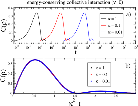
Figure 1: Energy conserving collective interaction $\lambda=\mu=\nu=0$. a) Concurrence a function of time for different $\kappa$ values as indicated in the legend. b) The same as a) but in the renormalized time $\kappa^{2}t$.

Our simulations (Figure 1a) show that, a concurrence of value approximately 0.3 is created, independently of the value of $\kappa$ (ranging from 0.01 to 1). It is clear from the graphs that the effect of varying $\kappa$ consists only in a time shift. This shift of time is particularly accurate, as can be seen in Fig. 1b, where the three curves drawn in a) collapse to a single curve under the time rescaling $t\to\kappa^{2}t$. In particular, the maximum concurrence is taken at times $t_{0}\approx 0.5\kappa^{-2}$. We also point out that the revived concurrence has very small amplitude (approximately 15 times smaller than the maximum concurrence) and takes its maximum at $t_{1}\approx 2.1\kappa^{-2}$. Even though the amplitude of the revived concurrence is small as compared to $\kappa^{2}$, the graphs show that it is independent of $\kappa$, and hence our resonance dynamics does reveal concurrence revival.

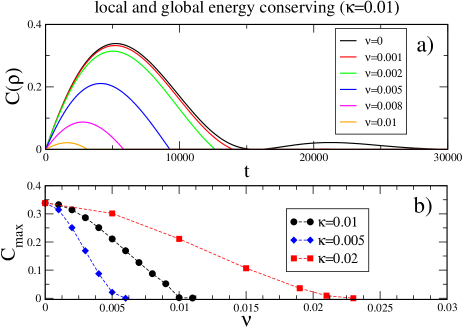
Figure 2: Energy conserving collective and local interaction $\lambda=\mu=0$. a) Concurrence a function of time for fixed collective interaction $\kappa=0.01$ and different local interaction $\nu$ as indicated in the legend. b) Variation of the maximum of concurrence as a function of the local interaction strength $\nu$ for different collective interaction strengths $\kappa$ as indicated in the legend.

When switching on the local energy conserving coupling, $\nu\neq 0$, we see in Fig. 2a, that the maximum of concurrence decreases with increasing $\nu$. Therefore, the effect of a local coupling is to reduce the entanglement. It is also interesting to study the dependence of the maximal value of the concurrence, $C_{\rm max}$, as a function of the energy-conserving interaction parameters. This is done in Fig. 2b, where $C_{\rm max}$ is plotted as a function of the local interaction $\nu$, for different fixed collective couplings $\kappa$. The graphs show that as the local coupling $\nu$ is increased to the value of the collective coupling $\kappa$, $C_{\rm max}$ becomes zero. This means that if the local coupling exceeds the collective one, then there is no creation of concurrence. We may interpret this as a competition between the concurrence-reducing tendency of the local coupling (apart from very small revival effects) and the concurrence-creating tendency of the collective coupling (for not too long times). If the local coupling exceeds the collective one, then concurrence is prevented from building up.

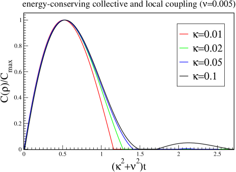
Figure 3: Energy conserving collective and local interaction $\lambda=\mu=0$. Rescaled concurrence $C(\rho)/C_{max}$ as function of time for fixed local interaction $\nu=0.005$ and different collective interaction $\kappa>\nu$ (as indicated in the legend) as a function of the rescaled time $(\kappa^{2}+\nu^{2})t$.

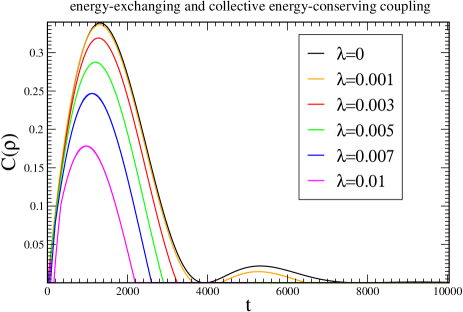
Figure 4: Energy-exchanging collective and local interactions $\lambda=\mu\neq 0$. Concurrence $C(\rho)$ as function of time for fixed energy-conserving collective interactions $\kappa=0.02$, $\nu=0$ and different energy-exchanging couplings $\lambda$ as indicated in the legend. Here we used $B_{1}=1$, $B_{2}=1.25$, and $\beta=1$.

Looking at Fig. 2, it is clear that the effect of the local coupling is not only to decrease concurrence but also to induce a shift of time, similarly to the effect of the collective coupling $\kappa$. Indeed, taking as a variable the rescaled concurrence $C(\rho)/C_{max}$, one can see that the approximate scaling $(\kappa^{2}+\nu^{2})t$ is at work, see Fig. 3. We conclude that both local and collective energy conserving interactions produce a cooperative time shift of the entanglement creation, but only the local interaction can destroy entanglement creation. There is no entanglement creation for $\nu>\kappa$.

Let us now consider an additional energy exchange coupling $\lambda,\mu\neq 0$. Since these parameters appear in the resonance dynamics only in the combination $\lambda^{2}+\mu^{2}$, see Appendix A, we set without loosing generality $\lambda=\mu$. We plot in Fig. 4 the time evolution of the concurrence, at fixed energy-conserving couplings $\kappa=0.02$ and $\nu=0$, for different values of the energy exchange coupling $\lambda$. In this case we have chosen $B_{1}=1$ which corresponds to $\omega_{0}=\omega_{1}/2$, where $\omega_{1}$ is a transition frequency of the first qubit. We also used the conditions: $\sigma_{g}(B_{1})=r_{g}(B_{1})=1$, which lead to the renormalization of the interaction constants. The relations between $\sigma_{g}(B_{2})$ and $\sigma_{g}(B_{1})$, and $r_{g}(B_{2})$ and $r_{g}(B_{1})$ are discussed in Appendix B.

Figure 4 shows that the effect of the energy exchanging coupling is to shift slightly the time where concurrence is maximal and, at the same time, to decrease the amplitude of concurrence for each fixed time. This feature is analogous to the effect of local energy-conserving interactions, as discussed above. Unfortunately, it is quite difficult in this case to extract the threshold values of $\lambda$ at which the creation of concurrence is prevented for all times. The difficulty comes from the fact that for larger values of $\lambda$, the concurrence is very small and the negative eigenvalues on order $O(\varkappa^{2})$ do not allow a reliable calculation. This picture does not change much if a local energy-conserving interaction $\nu<\kappa$ is added. In Fig. 5, we show respectively, the time shift of the maximal concurrence $\Delta t=t_{max}(\lambda)-t_{max}(\lambda=0)$ as a function of the energy-exchanging coupling $\lambda$ (a) and the behavior of the maximal concurrence as a function of the same parameter $\lambda$ for two different values of the local coupling $\nu$. Is appears evident that the role played by the energy-exchange coupling is very similar to that played by the local energy-conserving one.

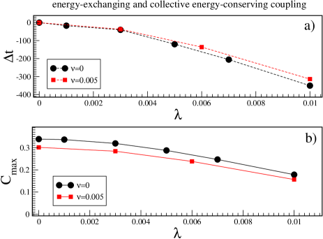
Figure 5: Energy-exchanging collective and local interaction $\lambda=\mu\neq 0$. a) Time shift induced by energy-exchanging coupling, for the same energy conserving collective coupling $\kappa=0.02$ and different local couplings $\nu$ as indicated in the legend. b) Decay of the maximal concurrence as a function of $\lambda$, for the same cases as (a). Magnetic fields and temperature is the same as in Fig. 4.

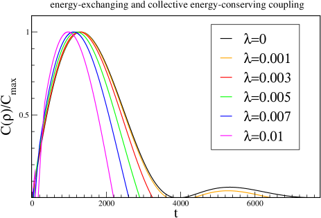
Figure 6: Energy-exchanging collective and local interaction $\lambda=\mu\neq 0$. Rescaled concurrence $C(\rho)/C_{max}$ vs time $t$, for different $\lambda$ values. Here,$\kappa=0.02$ and $\nu=0$. Magnetic fields and temperature is the same as in Fig. 4.

Let us comment about concurrence revival. The effect of a collective energy-conserving coupling consists of creating entanglement, destroying it and creating it again but with a smaller amplitude. Generally speaking, an energy-exchanging coupling, if extremely small, does not change this picture. Nevertheless, it is important to stress that the damping effect the energy-exchange coupling has on the concurrence amplitude is stronger on the revived concurrence than on the initially created one. This is shown in Fig. 6, where the renormalized concurrence $C(\rho)/C_{max}$ is plotted for different $\lambda$ values. For these parameter values, only a very small coupling $\lambda\leq 0.001$ will allow revival of concurrence.

In the calculation of concurrence, the square roots of the eigenvalues of the matrix $\xi(\rho)$ (6.2) should be taken. As explained before, the non positivity, to order $O(\varkappa^{2})$ of the density matrix $\rho$ reflects on the non positivity of the eigenvalues of the matrix $\xi(\rho)$. When this happens ($\nu_{i}<0$) we simply put $\nu_{i}=0$ in the numerical calculations. This produces an approximate (order $O(\varkappa^{2})$) concurrence which produces spurious effects, especially for small time, when concurrence is small. These effects are particularly evident in Fig. 6, for small time, where artificial oscillations occur, instead of an expected smooth behavior. In contrast to this behaviour, the revival of entanglement as revealed in Figure 6 varies smoothly in $\lambda$, indicating that this effect is not created due to the approximation.

9 Conclusion

We consider a system of two qubits interacting with local and collective thermal quantum reservoirs. Each qubit is coupled to its local reservoir by two channels, an energy-conserving and an energy-exchange one. The qubits are collectively coupled to a third reservoir, again through two channels. This is thus a versatile model, describing local and collective, energy-conserving and energy-exchange processes.

We present an approximate dynamics which describes the evolution of the reduced density matrix for all times $t\geq 0$, modulo an error term $O(\varkappa^{2})$, where $\varkappa$ is the typical coupling strength between a single qubit and a single reservoir. The error term is controlled rigorously and for all times. The approximate dynamics is markovian and shows that different parts of the reduced density matrix evolve together, but independently from other parts. This partitioning of the density matrix into clusters induces a classification of decoherence times – the time-scales during which a given cluster stays populated. We obtain explicitly the decoherence and relaxation times and show that their leading expressions (lowest nontrivial order in $\varkappa$) is independent of the ultraviolet behaviour of the system, and in particular, independent of any ultraviolet cutoff, artificially needed to make the models mathematically well defined.

We obtain analytical estimates on entanglement death and entanglement survival times for a class of initially entangled qubit states, evolving under the full, not explicitly solvable dynamics. We investigate numerically the phenomenon of entanglement creation and show that the approximate dynamics, even though it is markovian, does reveal creation, sudden death and revival of entanglement. We encounter in the numerical study a disadvantage of the approximation, namely that it is not positivity preserving, meaning that for small times, the approximate density matrix has slightly negative eigenvalues.

The above-mentioned cluster-partitioning of the density matrix is valid for general $N$-level systems coupled to reservoirs. We think this clustering will play a useful and important role in the analysis of quantum algorithms. Indeed, it allows one to separate “significant” from “insignificant” quantum effects, especially when dealing with large quantum registers for performing quantum algorithms. Depending on the algorithm, fast decay of some blocks of the reduced density matrix elements can still be tolerable for performing the algorithm with high fidelity.

We point out a further possible application of our method to novel quantum measuring technologies based on superconducting qubits. Using two superconducting qubits as measuring devices together with the scheme considered in this paper will allow one to extract not only the special density of noise, but also possible quantum correlations imposed by the environment. Modern methods of quantum state tomography will allow to resolve these issues.

Appendix A Dynamics in resonance approximation

We take $0<B_{1}<B_{2}$, $B_{2}/B_{1}\neq 2$, and $\varkappa^{2}<\!\!<\min\{2B_{1},2(B_{2}-B_{1}),2|B_{2}-2B_{1}|\}$. These conditions guarantee that the resonances do not overlap, see also [11]. In the sequel, $\doteq$ means equality modulo an error term $O(\varkappa^{2})$ which is homogeneous in $t\geq 0$. The main contribution of the dynamics in (3.10) is given as follows.

$${}[\rho_{t}]_{11} \doteq \frac{1}{Z}\frac{1}{\sqrt{e_{1}e_{2}}}\Big{\{}(1+{\rm e}^{-t\delta_{2}}e_{2}+{\rm e}^{-t\delta_{3}}e_{1}+{\rm e}^{-t\delta_{4}}e_{1}e_{2})[\rho_{0}]_{11}$$ (A.1)

$$\qquad+(1-{\rm e}^{-t\delta_{2}}+{\rm e}^{-t\delta_{3}}e_{1}-{\rm e}^{-t\delta_{4}}e_{1})[\rho_{0}]_{22}$$

$$\qquad+(1+{\rm e}^{-t\delta_{2}}e_{2}-{\rm e}^{-t\delta_{3}}e_{1}-{\rm e}^{-t\delta_{4}}e_{2})[\rho_{0}]_{33}$$

$$\qquad+(1-{\rm e}^{-t\delta_{2}}-{\rm e}^{-t\delta_{3}}-{\rm e}^{-t\delta_{4}})[\rho_{0}]_{44}\Big{\}}$$

$${}[\rho_{t}]_{22} \doteq \frac{1}{Z}\sqrt{\frac{e_{2}}{e_{1}}}\Big{\{}(1-{\rm e}^{-t\delta_{2}}+{\rm e}^{-t\delta_{3}}e_{1}-{\rm e}^{-t\delta_{4}}e_{1})[\rho_{0}]_{11}$$ (A.2)

$$\qquad+(1+{\rm e}^{-t\delta_{2}}e_{2}^{-1}+{\rm e}^{-t\delta_{3}}e_{1}+{\rm e}^{-t\delta_{4}}e_{1}e_{2}^{-1})[\rho_{0}]_{22}$$

$$\qquad+(1-{\rm e}^{-t\delta_{2}}-{\rm e}^{-t\delta_{3}}+{\rm e}^{-t\delta_{4}})[\rho_{0}]_{33}$$

$$\qquad+(1+{\rm e}^{-t\delta_{2}}e_{2}^{-1}-{\rm e}^{-t\delta_{3}}-{\rm e}^{-t\delta_{4}}e_{2}^{-1})[\rho_{0}]_{44}\Big{\}}$$

$${}[\rho_{t}]_{33} \doteq \frac{1}{Z}\sqrt{\frac{e_{1}}{e_{2}}}\Big{\{}(1+{\rm e}^{-t\delta_{2}}e_{2}-{\rm e}^{-t\delta_{3}}-{\rm e}^{-t\delta_{4}}e_{2})[\rho_{0}]_{11}$$ (A.3)

$$\qquad+(1-{\rm e}^{-t\delta_{2}}-{\rm e}^{-t\delta_{3}}+{\rm e}^{-t\delta_{4}})[\rho_{0}]_{22}$$

$$\qquad+(1+{\rm e}^{-t\delta_{2}}e_{2}+{\rm e}^{-t\delta_{3}}e_{1}^{-1}-{\rm e}^{-t\delta_{4}}e_{2}e^{-1}_{1})[\rho_{0}]_{33}$$

$$\qquad+(1-{\rm e}^{-t\delta_{2}}+{\rm e}^{-t\delta_{3}}e_{1}^{-1}-{\rm e}^{-t\delta_{4}}e_{1}^{-1})[\rho_{0}]_{44}\Big{\}}$$

$${}[\rho_{t}]_{44} \doteq \frac{1}{Z}\sqrt{e_{1}e_{2}}\Big{\{}(1-{\rm e}^{-t\delta_{2}}-{\rm e}^{-t\delta_{3}}+{\rm e}^{-t\delta_{4}})[\rho_{0}]_{11}$$ (A.4)

$$\qquad+(1+{\rm e}^{-t\delta_{2}}e_{2}^{-1}-{\rm e}^{-t\delta_{3}}-{\rm e}^{-t\delta_{4}}e_{2}^{-1})[\rho_{0}]_{22}$$

$$\qquad+(1-{\rm e}^{-t\delta_{2}}+{\rm e}^{-t\delta_{3}}e_{1}^{-1}-{\rm e}^{-t\delta_{4}}e^{-1}_{1})[\rho_{0}]_{33}$$

$$\qquad+(1+{\rm e}^{-t\delta_{2}}e_{2}^{-1}+{\rm e}^{-t\delta_{3}}e_{1}^{-1}+{\rm e}^{-t\delta_{4}}e_{1}^{-1}e_{2}^{-1})[\rho_{0}]_{44}\Big{\}}.$$

Here,

$$Z = {\rm Tr}{\rm e}^{-\beta H_{\rm S}},$$ (A.5)

$$e_{j} = {\rm e}^{2\beta B_{j}}$$ (A.6)

$$\delta_{2} = (\lambda^{2}+\mu^{2})\sigma_{g}(B_{2})$$ (A.7)

$$\delta_{3} = (\lambda^{2}+\mu^{2})\sigma_{g}(B_{1})$$ (A.8)

$$\delta_{4} = \delta_{2}+\delta_{3}.$$ (A.9)

Of course, the populations do not depend on any energy-conserving parameter. The cluster of matrix elements $\{(3,1),(4,2)\}$ evolves as

$${}[\rho_{t}]_{42} \doteq {\rm e}^{{\rm i}t\varepsilon_{2B_{1}}^{(1)}}\frac{e_{2}y_{+}}{1+e_{2}(y_{+})^{2}}\Big{\{}[\rho_{0}]_{31}+y_{+}[\rho_{0}]_{42}\Big{\}}$$ (A.10)

$$+{\rm e}^{{\rm i}t\varepsilon_{2B_{1}}^{(2)}}\frac{e_{2}y_{-}}{1+e_{2}(y_{-})^{2}}\Big{\{}[\rho_{0}]_{31}+y_{-}[\rho_{0}]_{42}\Big{\}},$$

$${}[\rho_{t}]_{31} \doteq {\rm e}^{{\rm i}t\varepsilon_{2B_{1}}^{(1)}}\frac{1}{1+e_{2}(y_{+})^{2}}\Big{\{}[\rho_{0}]_{31}+y_{+}[\rho_{0}]_{42}\Big{\}}$$ (A.11)

$$+{\rm e}^{{\rm i}t\varepsilon_{2B_{1}}^{(2)}}\frac{1}{1+e_{2}(y_{-})^{2}}\Big{\{}[\rho_{0}]_{31}+y_{-}{}[\rho_{0}]_{42}\Big{\}}.$$

Here,

$$\varepsilon_{2B_{1}}^{(k)}=A+\frac{1}{2}B(1+e_{2})-(-1)^{k}\frac{1}{2}\Big{[}B^{2}(1+e_{2})^{2}+4C(B(e_{2}-1)+C)\Big{]}^{1/2},$$ (A.12)

where

$$A = {\rm i}(\lambda^{2}+\mu^{2})\frac{1}{2}\sigma_{g}(B_{1})+{\rm i}(\kappa^{2}+\nu^{2})\sigma_{f}(0)-(\lambda^{2}+\mu^{2})r_{g}(B_{1})$$ (A.13)

$$B = {\rm i}(\lambda^{2}+\mu^{2})\sigma_{g}^{-}(B_{2})$$ (A.14)

$$C = -2\kappa^{2}r_{f}$$ (A.15)

$$y_{\pm} = 1+\frac{A+C-\varepsilon_{2B_{1}}^{(k)}}{e_{2}B}\qquad(k=1\ {\rm for}\ y_{+},\ k=2\ {\rm for}\ y_{-}).$$ (A.16)

and

$$\begin{array}[]{lll}\sigma_{g}(x)&=&\displaystyle 4\pi x^{2}\coth(\beta x)\int_{S^{2}}|g(2x,\Sigma)|^{2}{\rm d}\Sigma\\ &&\\ \sigma_{g}^{-}(x)&=&\displaystyle 2\pi x^{2}\frac{{\rm e}^{\beta x}}{\sinh(\beta x)}\int_{S^{2}}|g(2x),\Sigma)|^{2}{\rm d}\Sigma\\ &&\\ r_{g}(x)&=&\frac{1}{2}\ {\rm P.V.}\int_{{\mathbb{R}}\times S^{2}}u^{2}|g(|u|,\Sigma)|^{2}\coth(\beta|u|/2)\frac{1}{u-2x}{\rm d}u{\rm d}\Sigma\\ &&\\ r_{f}&=&{\rm P.V.}\displaystyle\int_{{\mathbb{R}}^{3}}\frac{|f|^{2}}{|k|}{\rm d}^{3}k\\ &&\\ \sigma_{f}(0)&=&\displaystyle 4\pi\lim_{x\downarrow 0}x^{2}\coth(\beta x)\int_{S^{2}}|f(2x),\Sigma)|^{2}{\rm d}\Sigma.\end{array}$$ (A.17)

The cluster of matrix elements $\{(2,1),(4,3)\}$ evolves as

$${}[\rho_{t}]_{21} \doteq {\rm e}^{{\rm i}t\varepsilon_{2B_{2}}^{(1)}}\frac{1}{1+e_{1}(y^{\prime}_{+})^{2}}\Big{\{}[\rho_{0}]_{21}+y^{\prime}_{+}[\rho_{0}]_{43}\Big{\}}$$ (A.18)

$$+{\rm e}^{{\rm i}t\varepsilon_{2B_{2}}^{(2)}}\frac{1}{1+e_{1}(y^{\prime}_{-})^{2}}\Big{\{}[\rho_{0}]_{21}+y_{-}[\rho_{0}]_{43}\Big{\}},$$

$${}[\rho_{t}]_{43} \doteq {\rm e}^{{\rm i}t\varepsilon_{2B_{2}}^{(1)}}\frac{e_{1}y^{\prime}_{+}}{1+e_{1}(y^{\prime}_{+})^{2}}\Big{\{}[\rho_{0}]_{21}+y^{\prime}_{+}[\rho_{0}]_{43}\Big{\}}$$ (A.19)

$$+{\rm e}^{{\rm i}t\varepsilon_{2B_{2}}^{(2)}}\frac{e_{1}y^{\prime}_{-}}{1+e_{1}(y^{\prime}_{-})^{2}}\Big{\{}[\rho_{0}]_{21}+y^{\prime}_{-}{}[\rho_{0}]_{43}\Big{\}}.$$

Here, $\varepsilon_{2B_{2}}^{(k)}$ is the same as $\varepsilon_{2B_{1}}^{(k)}$, but with all indexes labeling qubits 1 and 2 interchanged ($e_{1}\leftrightarrow e_{2}$, $B_{1}\leftrightarrow B_{2}$ in all coefficients involved in $\varepsilon_{2B_{1}}^{(k)}$ above). Also, $y^{\prime}_{\pm}$ is obtained from $y_{\pm}$ by the same switch of labels. Finally,

$${}[\rho_{t}]_{32} \doteq {\rm e}^{{\rm i}t\varepsilon_{2(B_{1}-B_{2})}}[\rho_{0}]_{32}$$ (A.20)

$${}[\rho_{t}]_{41} \doteq {\rm e}^{{\rm i}t\varepsilon_{2(B_{1}+B_{2})}}[\rho_{0}]_{41}$$ (A.21)

with

$$\varepsilon_{2(B_{1}-B_{2})} = {\rm i}(\lambda^{2}+\mu^{2})[\sigma_{g}(B_{1})+\sigma_{g}(B_{2})]+2{\rm i}\nu^{2}\sigma_{f}(0)$$

$$+(\lambda^{2}+\mu^{2})[r_{g}(B_{1})-r_{g}(B_{2})]$$

$$\varepsilon_{2(B_{1}+B_{2})} = {\rm i}(\lambda^{2}+\mu^{2})[\sigma_{g}(B_{1})+\sigma_{g}(B_{2})]+4{\rm i}\kappa^{2}\sigma_{f}(0)+2{\rm i}\nu^{2}\sigma_{f}(0)$$

$$-(\lambda^{2}+\mu^{2})[r_{g}(B_{1})+r_{g}(B_{2})].$$

Appendix B Reduction to independent parameters

The equations above contain four independent coupling constants $\lambda,\mu,\nu,\kappa$ describing the energy-conserving and the energy exchanging (local and collective) interaction, and eight different functions of the form factors $f$ and $g$ : $\sigma_{g}(B_{i})$, $r_{g}(B_{i})$, $\sigma_{g}^{-}(B_{i})$, $i=1,2$, $\sigma_{f}(0)$, $r_{f}$ (A.17).

These functions are not independent. First of all it is easy to see that the following relation holds:

$$\sigma_{g}^{-}(x)=\frac{e^{2\beta x}}{e^{2\beta x}+1}\sigma_{g}(x),$$ (B.1)

moreover, choosing for instance a form factor $g(2x,\Sigma)\propto\sqrt{2x}$ one has:

$$\frac{\sigma_{g}(B_{2})}{\sigma_{g}(B_{1})}=\left(\frac{B_{2}}{B_{1}}\right)^{3}\frac{\coth\beta B_{2}}{\coth\beta B_{1}}.$$ (B.2)

Integrals in $du$ in Eq. (A.17) converge only when adding a cut-off $u_{c}$. It is easy to show that, when $u_{c}\to\infty$ one has:

$$\lim_{u_{c}\to\infty}\frac{r_{g}(B_{2})}{r_{g}(B_{1})}=1,$$ (B.3)

and we can assume $r_{g}(B_{1})\simeq r_{g}(B_{2})$. So, we end up with four independent divergent integrals, $\sigma_{g}(B_{1}),\ r_{g}(B_{1}),\ \sigma_{f}(0),\ r_{f},$ in terms of which we can write explicitly the decay rates :

$$\begin{array}[]{lll}\alpha_{1}&=&(\lambda^{2}+\mu^{2})\sigma_{g}(B_{1})\\ &&\\ \alpha_{2}&=&(\lambda^{2}+\mu^{2})\sigma_{g}(B_{1})\left(\frac{B_{2}}{B_{1}}\right)^{3}\frac{\coth\beta B_{2}}{\coth\beta B_{1}}\\ &&\\ \alpha_{3}&=&\kappa^{2}\sigma_{f}(0)\\ &&\\ \alpha_{4}&=&\nu^{2}\sigma_{f}(0),\end{array}$$ (B.4)

and the Lamb shifts,

$$\begin{array}[]{lll}\beta_{1}&=&(\lambda^{2}+\mu^{2})r_{g}(B_{1})\\ &&\\ \beta_{2}&=&(\lambda^{2}+\mu^{2})r_{g}(B_{2})\simeq\beta_{1}\\ &&\\ \beta_{3}&=&-\kappa^{2}r_{f}.\end{array}$$ (B.5)

Suppose now that both Lamb shifts, and decay constants are experimentally measurable quantities, and also assume (due to symmetry) that $\lambda=\mu$. Interaction constants can be renormalized in order to give directly decay constants and Lamb shifts:

$$\begin{array}[]{lll}\alpha_{1}&=&2\tilde{\lambda}^{2}\\ &&\\ \alpha_{2}&=&2\tilde{\lambda}^{2}\left(\frac{B_{2}}{B_{1}}\right)^{3}\frac{\coth\beta B_{2}}{\coth\beta B_{1}}\\ &&\\ \alpha_{3}&=&\tilde{\kappa}^{2}\\ &&\\ \alpha_{4}&=&\tilde{\nu}^{2},\\ \beta_{1}&=&2\tilde{\lambda}^{2}\\ &&\\ \beta_{2}&=&\beta_{1}\\ &&\\ \beta_{3}&=&-\tilde{\kappa}^{2}.\end{array}$$ (B.6)

$\tilde{\lambda},\ \tilde{\kappa},\tilde{\nu}$ are the values chosen for simulations.

References

- [1] T. Yu and J. H. Eberly, Qubit disentanglement and decoherence via dephasing, Phys. Rev. B, 68, 165322-1-9 (2003), Yu, T., Eberly, J.H.: Finite-Time Disentanglement Via Spontaneous Emission. Phys. Rev. Lett. 93, no.14, 140404 (2004); Sudden Death of Entanglement. Sience, 323, 598-601, 30 January 2009; Sudden death of entanglement: Classical noise effects. Optics Communications, 264, 393-397 (2005).
- [2] J. Wang, H. Batelaan, J. Podany, and A.F Starace, Entanglement evolution in the presence of decoherence, J. Phys. B: At. Mol. Opt. Phys. 39, 4343-4353 (2006).
- [3] L. Amico, R. Fazio, A. Osterloh, and V. Vedral, Entanglement in many-body systems, Rev. Mod. Phys., 80, 518- 576 (2008).
- [4] O.J. Faŕias, C.L. Latune, S.P. Walborn, L. Davidovich, and P.H.S. Ribeiro, Determining the dynamics of entanglement, SCIENCE, 324, 1414-1417 (2009).
- [5] Y. Makhlin, G. Schön, and A. Shnirman, Quantum-state engineering with Josephson-junction devices, Rev. Mod. Phys., 73, 380-400 (2001).
- [6] Y. Yu, S. Han, X. Chu, S.I Chu, Z. Wang, Coherent temporal oscillations of macroscopic quantum states in a Josephson junction, SCIENCE, 296, 889-892 (2002).
- [7] M.H. Devoret and J.M. Martinis, Implementing qubits with superconducting integrated circuits, Quantum Information Processing, 3, 163-203 (2004).
- [8] M. Steffen, M. Ansmann, R. McDermott, N. Katz, R.C. Bialczak, E. Lucero, M. Neeley, E.M. Weig, A.N. Cleland, and J.M. Martinis, State tomography of capacitively shunted phase qubits with high fidelity, Phys. Rev. Lett. 97 050502-1-4 (2006).
- [9] N. Katz, M. Neeley, M. Ansmann, R.C. Bialczak, M. Hofheinz, E. Lucero, A. O’Connell, Reversal of the weak measurement of a quantum state in a superconducting phase qubit, Phys. Rev. Lett., 101, 200401-1-4 (2008).
- [10] A.A. Clerk, M.H. Devoret, S.M. Girvin, Florian Marquardt, and R.J. Schoelkopf, Introduction to quantum noise, measurement and amplification, Preprint arXiv:0810.4729v1 [cond-mat] (2008).
- [11] M. Merkli, I.M. Sigal, G.P. Berman: Decoherence and thermalization. Phys. Rev. Lett. 98 no. 13, 130401, 4 pp (2007); Resonance theory of decoherence and thermalization. Ann. Phys. 323, 373-412 (2008); Dynamics of collective decoherence and thermalization. Ann. Phys. 323, no. 12, 3091-3112 (2008).
- [12] M. Merkli: Entanglement Evolution, a Resonance Approach. Preprint 2009.
- [13] G.M. Palma, K.-A. Suominen, A.K. Ekert: Quantum Computers and Dissipation. Proc. R. Soc. Lond. A 452, 567-584 (1996).
- [14] M. Merkli: Level shift operators for open quantum systems. J. Math. Anal. Appl. 327, Issue 1, 376-399 (2007).
- [15] H.-P. Breuer, F. Petruccione: The theory of open quantum systems. Oxford university press 2002.
- [16] B. Bellomo, R. Lo Franco, G. Compagno: Non-Markovian Effects on the Dynamics of Entanglement. Phys. Rev. Lett. 99, 160502 (2007).
- [17] A.J. Leggett, S. Chakravarty, A.T. Dorsey, Matthew P.A. Fisher, Anupam Garg, W. Zwerger: Dynamics of the dissipative two-state system. Rev. Mod. Phys. 59, 1–85 (1987).
- [18] A. Shnirman, Yu. Makhlin, G. Schön: Noise and Decoherence in Quantum Two-Level Systems. Physica Scripta T102, 147-154 (2002).
- [19] U. Weiss: Quantum dissipative systems. 2nd edition, World Scientific, Singapore, 1999.
- [20] C.H. Bennett, D.P. Divincenzo, J.A. Smolin, W.K. Wootters: Mixed-state entanglement and quantum error correction. Phys. Rev. A, 54, no.5, 3824-3851 (1996).
- [21] W.K. Wootters: Entanglement of Formation of an Arbitrary State of Two Qubits. Phys. Rev. Lett. 80, no. 10, 2245-2248 (1998).
- [22] J.-H. Huang, S.-Y. Zhu: Sudden death time of two-qubit entanglement in a noisy environment. Optics Communications, 281, 2156-2159 (2008).
- [23] J.P. Paz, A.J. Roncaglia: Dynamics of the entanglement between two oscillators in the same environment. Preprint arXiv:0801.0464v1.
- [24] D. Braun: Creation of Entanglement by Interaction with a Common Heat Bath. Phys. Rev. Lett. 89, 277901 (2002).
- [25] A. Peres: Separability Criterion for Density Matrices. Phys. Rev. Lett. 77, 1413–1415 (1996).
- [26] M. Horodecki, P. Horodecki, R. Horodecki: Separability of Mixed States: Necessary and Sufficient Conditions. Physics Letters A 223, 1-8 (1996).